Light higgsino-dominated NLSPs in semi-constrained NMSSM

1. Introduction

• 1. Introduction
• 2. Introduction to NMSSM and scNMSSM
•      2.1 Higgs sector of NMSSM and scNMSSM
•      2.2 Electroweakino sector of NMSSM and scNMSSM
• 3. Light Higgsino-dominated NLSPs in scNMSSM
•      3.1 Constraints from direct SUSY searches with CheckMATE
•      3.2 Production and decay of Higgsino-dominated NLSPs
•      3.3 Possibility of future discovery at HL-LHC
• 4. Conclusions

As an internal symmetry between fermions and bosons, supersymmetry (SUSY) is an attractive concept. In the framework of SUSY, the strong, weak, and hypercharge gauge couplings ($g_3,\; g_2,\; g_1$) can be unified at the GUT scale ($\sim 10^{16} \; {{\rm{GeV}}}$), and the large hierarchy problem between the electroweak and the Planck scales can be resolved. Further, with the R-parity conserved, the lightest SUSY particle (LSP) is stable and can be a good candidate for weakly-interacting-massive-particle (WIMP) dark matter (DM).

SUSY at the TeV scale is motivated by possible cancellation of quadratic divergences of the Higgs boson mass. The simplest implementation of SUSY is the minimal supersymmetric extension to the standard model (MSSM). Since the soft SUSY breaking parameters are totally free in the MSSM, a dynamic approach to obtain these parameters is more favored. In the minimal supergravity (mSUGRA), the Käler potential is employed to yield minimal kinetic energy terms for MSSM fields, where all trilinear couplings, gaugino, and scalar mass parameters unify respectively at the GUT scale. The fully constrained MSSM (CMSSM) is the MSSM with the boundary conditions that are the same as in the mSUGRA. However, to obtain a 125 GeV SM-like Higgs, the MSSM requires large one-loop radiative corrections to the Higgs mass, which renders the MSSM not natural. There is a so-called $\mu$-problem [1] in the MSSM, where the superpotential contains a term $\mu \hat{H}_u \hat{H}_d$, and $\mu$ is the only dimensionful parameter, which has to be chosen artificially.

The next-to minimal supersymmetric standard model (NMSSM) solves the $\mu$-problem by introducing a complex singlet superfield $\hat{S}$, which dynamically generates an effective $\mu$-term. This predicts an SM-like 125 GeV Higgs under all constraints and with low fine-tuning [2, 3]. The fully constrained NMSSM (cNMSSM) contains none or only one more parameter than the CMSSM/mSUGRA, thus both of them are in tension with current experimental constraints including 125 GeV Higgs mass, high mass bound of gluino, muon g-2, and dark matter [4–23]. Hence, we consider the semi-constrained NMSSM (scNMSSM) that relaxes the unification of scalar masses by decoupling the square-masses of the Higgs bosons and the squarks/sleptons, which is also referred to as NMSSM with non-universal Higgs mass (NUHM) [24-26]. In the scNMSSM, the bino and wino are heavy because the high mass bound of gluino and the unification of gaugino masses at GUT scale, thus the light neutralinos and charginos can only be singlino-dominated or higgsino-dominated^①.

In recent years, ATLAS and CMS collaborations have carried out numerous searches for SUSY particles, which pushed the gluino and squarks masses bounds in simple models up to several hundred GeV and even the TeV scale. Meanwhile, it remains possible for the electroweakino sector to be very light. The electroweakino sector of NMSSM was studied in [27-44], among which different search channels were provided, such as multi-leptons [35, 36] and jets with missing transverse momentum (${{\not\!\!\!{\overrightarrow{p}}} _T}$) [37]. These motivated us to verify the current status of higgsino in special SUSY models such as the scNMSSM, under direct-search constraints and their possibility of discovery by detailed simulation.

In this study, we discuss the light higgsino-dominated NLSPs (next-to-lightest supersymmetric particles) in the scNMSSM. We use the scenario of singlino-dominated $\tilde{\chi}^0_1$ and SM-like $h_2$ in the scan result in our former work on scNMSSM [26], where we considered the constraints including theoretical constraints of vacuum stability and Landau pole, experimental constraints of Higgs data, muon g-2, B physics, dark matter relic density, and direct searches, etc. Thus, in this scenario the $\tilde{\chi}^{\pm}_1$ and $\tilde{\chi}^0_{2,3}$ are higgsino-dominated, light and mass-degenerated NLSPs. We first investigate the constraints on these NLSPs, including searching for SUSY particles at the LHC Run-I and Run-II. We employ Monte Carlo algorithm to perform detailed simulations to impose these constraints. Then, we discuss the possibility of discovering the higgsino-dominated NLSPs in the future at the high-luminosity LHC (HL-LHC).

This paper is organized as follows. First, in Section 2, we briefly introduce the model of NMSSM and scNMSSM, especially in the Higgs and electroweakino sector. Later in Section 3, we discuss the constraints to the light higgsino-dominated NLSPs, and the possibility of discovering them at the HL-LHC. Finally, we draw our conclusions in Section 4.

2. Introduction to NMSSM and scNMSSM

• 1. Introduction
• 2. Introduction to NMSSM and scNMSSM
•      2.1 Higgs sector of NMSSM and scNMSSM
•      2.2 Electroweakino sector of NMSSM and scNMSSM
• 3. Light Higgsino-dominated NLSPs in scNMSSM
•      3.1 Constraints from direct SUSY searches with CheckMATE
•      3.2 Production and decay of Higgsino-dominated NLSPs
•      3.3 Possibility of future discovery at HL-LHC
• 4. Conclusions

The superpotential of NMSSM with $\mathbb{Z}_3$ symmetry :

where superfields $\hat{H}_u$ and $\hat{H}_d$ are two complex doublet superfields, superfield $\hat{S}$ is the singlet superfield, coupling constants $\lambda$ and $\kappa$ are dimensionless, and $W_{\rm MSSM}|_{\mu = 0}$ presents the Yukawa couplings of the $\hat{H}_u$ and $\hat{H}_d$ to the quark and lepton superfields. In electroweak symmetry breaking, the scalar component of superfields $\hat{H}_u$, $\hat{H}_d$, and $\hat{S}$ obtain their vacuum expectation values (VEVs) $v_u$, $v_d$, and $v_s$ respectively. The relations between the VEVs are

where the $\mu_{\rm eff}$ is the mass scale of a higgsino, like in the MSSM. In the following, for the sake of convenience, we refer to $\mu_{\rm eff}$ as $\mu$.

The soft SUSY breaking terms in the NMSSM are only different from the MSSM in several terms:

where S, $H_u$, and $H_d$ are the scalar components of the superfields, the ${m}_S^2$ is the soft SUSY breaking mass for singlet field S, and the trilinear coupling constants $A_\lambda$ and $A_\kappa$ have a mass dimension.

In the semi-constrained NMSSM (scNMSSM), the Higgs sector are considered non-universal, that is, the Higgs soft mass $m^2_{H_u}$, $m^2_{H_d}$, and $m^2_{S}$ are allowed to be different from $M^2_0+\mu^2$, and the trilinear couplings $A_\lambda$, $A_\kappa$ can be different from $A_0$. Hence, in the scNMSSM, the complete parameter sector is usually chosen as:

2.1 Higgs sector of NMSSM and scNMSSM

• 1. Introduction
• 2. Introduction to NMSSM and scNMSSM
•      2.1 Higgs sector of NMSSM and scNMSSM
•      2.2 Electroweakino sector of NMSSM and scNMSSM
• 3. Light Higgsino-dominated NLSPs in scNMSSM
•      3.1 Constraints from direct SUSY searches with CheckMATE
•      3.2 Production and decay of Higgsino-dominated NLSPs
•      3.3 Possibility of future discovery at HL-LHC
• 4. Conclusions

When the electroweak symmetry breaks, the scalar component of superfields $\hat{H}_u$, $\hat{H}_d$, and $\hat{S}$ can be written as

where $H^R_u$, $H^R_d$, and $S^R$ are CP-even component fields, $H^I_u$, $H^I_u$, and $S^I$ are the CP-odd component fields, and the $H^+_u$ and $H^-_d$ are charged component fields

On the basis of $(H^R_d, H^R_u, S^R)$, the CP-even scalar mass matrix is [45]

with

where

and $s_{\beta} = \sin\beta, c_{\beta} = \cos\beta$. Indeed, here is a more common basis $(H_1, H_2, S^R)$, where

and the $H_2$ is the SM Higgs field. On the basis of $(H_1, H_2, S^R)$, the scalar mass matrix is different from Eq. (7). However, since the rotation of the basis does not touch the third component $S^R$, the $M_{S, S^R S^R}^2$ will remain the same as in Eq. (10). The Higgs boson mass matrix $M_{S'}^2$ on basis $(H_1, H_2, S^R)$ is given by [46]

And comparing Eq. (17) with Eq. (10), it's not hard to get $M_{S',S^R S^R}^2 = M_{S,S^R S^R}^2$.

To obtain the physical CP-odd scalar Higgs bosons, the Higgs fields may be rotated,

Subsequently, the Goldstone mode is dropped off, and the CP-odd scalar mass matrix on the basis of $(A, S^I)$ becomes [45]

with

where

The mass eigenstates of the CP-even Higgs $h_i$ ($i = 1,2,3$) and the CP-odd Higgs $A_i$($i = 1,2$) are obtained by

where the matrix $S_{ij}$ can diagonalize the mass matrix $M_{S'}^2$, and the matrix $P_{ij}$ can diagonalize the mass matrix $M_{P}^2$.

2.2 Electroweakino sector of NMSSM and scNMSSM

• 1. Introduction
• 2. Introduction to NMSSM and scNMSSM
•      2.1 Higgs sector of NMSSM and scNMSSM
•      2.2 Electroweakino sector of NMSSM and scNMSSM
• 3. Light Higgsino-dominated NLSPs in scNMSSM
•      3.1 Constraints from direct SUSY searches with CheckMATE
•      3.2 Production and decay of Higgsino-dominated NLSPs
•      3.3 Possibility of future discovery at HL-LHC
• 4. Conclusions

In the NMSSM, there are five neutralinos $\tilde{\chi}^0_{i}$ ($i = 1,2,3,4,5$), which are a mixture of $\tilde{B}$ (bino), $\tilde{W}^{3}$ (wino), $\tilde{H}_{d}^0$, $\tilde{H}_{u}^0$ (higgsinos), and $\tilde{S}$ (singlino). On the gauge-eigenstate basis $\psi^0 = (\tilde{B}, \tilde{W}^{3}, \tilde{H}_{d}^0, \tilde{H}_{u}^0, \tilde{S})$, the neutralino mass matrix takes the form [45]

where $s_{\beta} = \sin\beta, c_{\beta} = \cos\beta, s_W = \sin\theta_W, c_W = \cos\theta_W$. To obtain the mass eigenstates, one may diagnolize the neutralino mass matrix $M_{\tilde{\chi}^{0}}$

where $M_{\tilde{\chi}^{0}}^{D}$ is the diagonal mass matrix, and the order of eigenvalues is $m_{\tilde{\chi}^0_{\rm 1}}<m_{\tilde{\chi}^0_{\rm 2}}<m_{\tilde{\chi}^0_{\rm 3}}<m_{\tilde{\chi}^0_{\rm 4}}<m_{\tilde{\chi}^0_{\rm 5}}$. Meanwhile, the mass eigenstates are obtained

In the scNMSSM, bino and wino were constrained to be very heavy because of the high mass bounds of gluino and the universal gaugino mass at the GUT scale. Thus, they can be decoupled from the light sector. Then, the following relations for the $N_{ij}$ are found [47, 48]:

We assume that the lightest neutralino $\tilde{\chi}^0_{\rm 1}$ is the lightest supersymmetric particle (LSP) and makes up of the cosmic dark matter. If the LSP $\tilde{\chi}^0_{\rm 1}$ satisfies $N_{15}^2 > 0.5$, we call it singlino-dominated. The coupling of such an LSP with the CP-even Higgs bosons is given by [47, 48]

In the singlino-dominated-LSP scenario, assuming $N_{11} = N_{12} = 0$, the mass of LSP can be written as $m_{\tilde{\chi}^0_{\rm 1}} \approx M_{\tilde{\chi}^{0},\tilde{S} \tilde{S} } = 2 \kappa v_s$. From Eq. (23), Eq. (10), and Eq. (21), one can find the sum rule [49, 50]:

In the case where $h_1$ singlet-like, $\tan\beta$ sizable, $\lambda, \kappa$, and $A_\lambda$ are not too large, this equation can become

The chargino sector in the NMSSM is similar to the neutralino sector. The charged higgsino $\tilde{H}_u^+$, $\tilde{H}_d^-$ (with mass scale $\mu$) and the charged gaugino $\tilde{W}^{\pm}$ (with mass scale $M_2$) can combine, forming two couples of physical chargino $\chi_1^{\pm}, \, \chi_2^{\pm}$. On the gauge-eigenstate basis $(\tilde{W}^+, \tilde{H}_{u}^+, \tilde{W}^-, \tilde{H}_{d}^-)$, the chargino mass matrix is given by [45]

To obtain the chargino mass eigenstates, one can use two unitary matrices to diagonalize the chargino mass matrix by

where $M_{\tilde{\chi}^{\pm}}^{D}$ indicates the diagonal mass matrix, and the order of eigenvalues is $m_{\tilde{\chi}^{\pm}_{\rm 1}}<m_{\tilde{\chi}^{\pm}_{\rm 2}}$. Meanwhile, we obtain the mass eigenstates

In the scNMSSM, since $M_2\gg \mu$, $\chi^\pm_1$ can be higgsino-dominated, with a mass of approximately $\mu$. With $\chi^0_1$ is singlino-dominated, $\chi^0_{2,3}$ can be higgsino-dominated, with masses that are nearly degenerate and approximately $\mu$ and $N_{23}^2+N_{24}^2 > 0.5$. When $\mu$ is not large, i.e., smaller than the mass of other particles, the nearly-degenerate $\chi^\pm_1$ and $\chi^0_{2,3}$ are referred to as the next-to-lightest SUSY particles (NLSPs). In this study, we focus on the detection of the higgsino-dominated NLSPs ($\chi^\pm_1$ and $\chi^0_{2,3}$) in the scNMSSM.

3. Light Higgsino-dominated NLSPs in scNMSSM

• 1. Introduction
• 2. Introduction to NMSSM and scNMSSM
•      2.1 Higgs sector of NMSSM and scNMSSM
•      2.2 Electroweakino sector of NMSSM and scNMSSM
• 3. Light Higgsino-dominated NLSPs in scNMSSM
•      3.1 Constraints from direct SUSY searches with CheckMATE
•      3.2 Production and decay of Higgsino-dominated NLSPs
•      3.3 Possibility of future discovery at HL-LHC
• 4. Conclusions

We employ the scan result from our previous study on scNMSSM [26]; however, we only consider the surviving samples with singlino-dominated $\chi^0_1$ ($|N_{15}|^2>0.5$) as the LSP, and impose the SUSY search constraints with ${\textsf{CheckMATE}}$ [51–53]. We perform the scan with the program ${\textsf{NMSSMTools-5.4.1}}$ [54-57], and considered the constraints there, including theoretical constraints of vacuum stability and the Landau pole, experimental constraints of Higgs data, muon g-2, B physics, dark matter relic density, and direct searches, etc^②. We also use ${\textsf{HiggsBounds-5.1.1beta}}$ [58] to constrain the Higgs sector (with $h_2$ as the SM-like Higgs and $123<m_{h_2}<127 \; {{\rm{GeV}}}$), and ${\textsf{SModelS-v1.1.1} }$ [59, 60] to constrain SUSY particles. The detail of the constraints can be found in Ref. [26]. The scanned spaces of the parameters are:

As shown in Ref. [26], in the surviving parameter space,

● The glugino is heavier than 1.5 TeV, i.e., $M_{1/2}$ at GUT scale, or $M_3/2.4\simeq M_2/0.8 \simeq M_1/0.4$ at $M_{\rm SUSY}$ scale due to RGE runnings, and it is larger than approximately $700 \; {{\rm{GeV}}}$.

● Because of RGE runnings, including $M_3$, the squarks can be heavy. Even the lightest squarks, e.g., $\tilde{t}_1$, are heavier than approximately $500 \; {{\rm{GeV}}}$.

● Because of RGE runnings, including $M_2$ and $M_1$, the sleptons of the first two generations and all neutrinos are heavier than approximately $300 \; {{\rm{GeV}}}$, only $\tilde{\tau}_1$ can be lighter, at approximately $100 \; {{\rm{GeV}}}$.

● The heavy charginos $\tilde{\chi}^\pm_2$ are wino-like and heavier than approximately $560 \; {{\rm{GeV}}}$, the light charginos $\tilde{\chi}^\pm_1$ are higgsino-like at $100\sim200 \; {{\rm{GeV}}}$.

● For the five neutralinos, $\tilde{\chi}^0_5$ is wino-like and heavier than $560 \; {{\rm{GeV}}}$, the bino-dominated neutralino is heavier than $280 \; {{\rm{GeV}}}$, the higgsino-dominated neutralinos are $100\sim200 \; {{\rm{GeV}}}$, while the singlino-dominated neutralino can be $60\sim400 \; {{\rm{GeV}}}$.

● For the Higgs sector, $h_2$ represents the SM-like Higgs at $123\sim127 \; {{\rm{GeV}}}$, $h_1$ is singlet-dominated and lighter than $123 \; {{\rm{GeV}}}$, the light CP-odd Higgs is singlet-dominated, but it can be lighter or heavier than $125 \; {{\rm{GeV}}}$. Since $h_2$ is SM-like, the Higgs invisible decay caused by $m_{\tilde{\chi}^0_1}\simeq 60 \; {{\rm{GeV}}}$ is at most about 20%, so as the Higgs exotic decays caused by $m_{h_1,a_1}\lesssim60 \; {{\rm{GeV}}}$.

In this study, we choose the surviving samples with $\tilde{\chi}^0_1$ LSP as singlino-dominated, and higgsino-dominated neutralino and chargino ($\tilde{\chi}^\pm_1$ and $\tilde{\chi}^0_{2,3}$) as NLSPs. Thus, the samples with higgsino-dominated neutralinos as LSPs, or $\tilde{\tau}_1$ as NLSP, are discarded. In the following, we focus on the higgsino-dominated NLSPs in the scNMSSM, considering its constraints from direct search results at the LHC Run I and Run II, its production and decay, and its possibility of discovery at the HL-LHC in the future.

3.1 Constraints from direct SUSY searches with CheckMATE

• 1. Introduction
• 2. Introduction to NMSSM and scNMSSM
•      2.1 Higgs sector of NMSSM and scNMSSM
•      2.2 Electroweakino sector of NMSSM and scNMSSM
• 3. Light Higgsino-dominated NLSPs in scNMSSM
•      3.1 Constraints from direct SUSY searches with CheckMATE
•      3.2 Production and decay of Higgsino-dominated NLSPs
•      3.3 Possibility of future discovery at HL-LHC
• 4. Conclusions

Furthermore, we use ${\texttt{CheckMATE 2.0.26}}$ [51–53] to impose these constraints of direct SUSY search results at the LHC, using all data at Run I and up to $36 {\; {\rm{fb}}}^{-1}$ data at Run II [61–66]. For masses of $100 \sim 200$ GeV, the cross-sections of the higgsino-dominated NLSPs can be sizeable, thus we pay special attention to the NLSPs.

First, We use ${\texttt{MadGraph5}}\_{\texttt{aMC@NLO 2.6.6}}$ [67] to generate three types of tree level processes at 8 TeV and 13 TeV:

Since the cross-sections by the ${\texttt{MadGraph}}$ are at the tree level, we multiply them by a NLO K-factor calculated with the ${\texttt{Prospino2}}$ [68]. Then, we use ${\texttt{PYTHIA 8.2}}$ [69] to deal with particle decay, parton showering, and hardronization, and we use ${\texttt{Delphes 3.4.1}}$ [70] to simulate the detector response. The anti-$k_T$ algorithm [71] is employed for jet clustering.

After the simulation, we obtain a ‘.root’ file. We use the ${\texttt{CheckMATE2}}$ to read this ‘.root’ file. Then, we apply the same cuts in signal regions of the CMS and ATLAS experiments at 8 TeV and 13 TeV, using analysis cards that have been implemented in ${\texttt{CheckMATE2}}$. At the last step, with the ${\texttt{CheckMATE2}}$, we obtain an r-value for each sample, which is defined as

where S is the total number of expected signal events, $\Delta S$ is the uncertainty of S, and $S_{\rm Exp.}^{95}$ is the experimentally measured at the 95% confidence limit of the signal events number. Hence, a model can be considered excluded at the 95% confidence level, if $r \geqslant 1$. If the $r \geqslant 1$ in only one signal region, the model can also be excluded. We obtain $r_{\max}$, the maximal value of r in different signal regions. The model is excluded if $r_{\max} \geqslant 1$.

After using ${\texttt{CheckMATE}}$ to verify our surviving samples, we note that most of the samples excluded are by the CMS analysis in multilepton final states at 13 TeV LHC with $35.9 {\; {\rm{fb}}}^{-1}$ data [61-64, 72]^③. We confirmed that the relevant mechanism is $\tilde{\chi}_1^{\pm} \tilde{\chi}_2^{0}$ produced and each decaying to two bodies. Since the sleptons are heavier, the $\tilde{\chi}_1^{\pm}$ and $\tilde{\chi}_2^{0}$ mainly decay to $\tilde{\chi}_1^{0}$ LSP plus a W, or Z, or Higgs boson. The most effective processes excluding the samples are $pp\to \tilde{\chi}_1^{\pm}(W^{\pm}\tilde{\chi}_1^{0}) \tilde{\chi}_2^{0} (Z\tilde{\chi}_1^{0})$ and $pp\to \tilde{\chi}_1^{\pm}(W^{\pm}\tilde{\chi}_1^{0}) \tilde{\chi}_2^{0} (h_2\tilde{\chi}_1^{0})$.

The search strategy for these two processes is three or more leptons and a large ${{\not\!\!\! {\overrightarrow{p}}} _T}$ in the final state, since these channels are relatively cleaner than the jet channels at the LHC. The CMS searches related to our processes include the following signal regions (SR) SR-A, SR-C, and SR-F

● SR-A: events with three light leptons (e or $\mu$), two of which form an opposite sign same-flavor (OSSF) pair. The SR-A is divided into 44 bins, according to the invariant mass of an OSSF pair $M_{\ell \ell}$, third lepton's transverse mass $M_T$, and missing transverse momentum ${{\not\!\!\!{\overrightarrow{p}}} _T}$. The transverse mass $M_T$ is defined as

where $\Delta\phi$ is the angle between ${\vec p}_T^{\ell}$ and ${{\not\!\!\! {\overrightarrow{p}}} _T}$.

● SR-C: events with two light leptons (e or $\mu$) forming an OSSF pair, and one ${\rm{\tau}} _{h}$ candidate. The SR-C is divided into 18 bins, according to the invariant mass $M_{\ell \ell}$, the two-lepton ‘stransverse mass’ $M_{T2}(\ell_1, \ell_2)$ [73-75] instead of $M_T$ on the off-Z regions, and the ${{\not\!\!\! {\overrightarrow{p}}} _T}$. The $M_{T2}$ is defined as

where $\vec{p}_T^{\ell_1}$ and $\vec{p}_T^{\ell_2}$ are the transverse momenta for the two leptons, respectively, while ${\not\!\!\! {\overrightarrow{p}}} _T^1$ and ${\not\!\!\! {\overrightarrow{p}}} _T^2$ depict the random two components of the missing transverse momenta ${{\not\!\!\! {\overrightarrow{p}}} _T}$. This is used to suppress the SM background, since the large $t\bar{t}$ background is at low $M_{T2}$.

● SR-F: events with one light lepton (e or $\mu$) plus two ${\rm{\tau }}_{h}$ candidates. SR-F is divided into 12 bins, according to $M_{\ell \ell}$, $M_{T2}(\ell, {\rm{\tau }}_{1})$, and the ${{\not\!\!\! {\overrightarrow{p}}} _T}$.

Recently after 2017, ATLAS and CMS collaborations have released several new search results with more Run-II data up to $139 {\; {\rm{fb}}}^{-1}$ in channels as $2\ell+ {\not\!\!\! {\overrightarrow{p}}}_T$ [76-81], $3\ell+ {\not\!\!\! {\overrightarrow{p}}}_T$ [72] (see also non-SUSY interpretations of multilepton anomalies in Refs. [82–84]), $2\gamma+ {\not\!\!\! {\overrightarrow{p}}}_T$ [85, 86], Higgs$+ {\not\!\!\! {\overrightarrow{p}}}_T$ [87], and Higgs$+\ell+ {\not \!\!\!{\overrightarrow{p}}}_T$ [88], and for compressed mass spectrum [89, 90]. In their analyses, they considered simple models, where purely higgsino or wino NLSP produced in pair, each decaying to $\tilde{\chi}^0_1$ plus h, Z, or $W^\pm$ in 100%, such that the results do not apply to our samples directly. Imposing these new constraints is complex, and we plan to address them in our future studies.

3.2 Production and decay of Higgsino-dominated NLSPs

• 1. Introduction
• 2. Introduction to NMSSM and scNMSSM
•      2.1 Higgs sector of NMSSM and scNMSSM
•      2.2 Electroweakino sector of NMSSM and scNMSSM
• 3. Light Higgsino-dominated NLSPs in scNMSSM
•      3.1 Constraints from direct SUSY searches with CheckMATE
•      3.2 Production and decay of Higgsino-dominated NLSPs
•      3.3 Possibility of future discovery at HL-LHC
• 4. Conclusions

For the surviving samples, we first investigated the production cross-sections of $\tilde{\chi}_1^{+} \tilde{\chi}_2^{0}$, $\tilde{\chi}_1^{+} \tilde{\chi}_3^{0}$, $\tilde{\chi}_1^{-} \tilde{\chi}_2^{0}$, $\tilde{\chi}_1^{-} \tilde{\chi}_3^{0}$, $\tilde{\chi}_1^{+} \tilde{\chi}_1^{-}$, $\tilde{\chi}_2^{0} \tilde{\chi}_3^{0}$, $\tilde{\chi}_2^{0} \tilde{\chi}_2^{0}$, and $\tilde{\chi}_3^{0} \tilde{\chi}_3^{0}$ at the 14 TeV LHC. Since the NLSPs are higgsino-dominated, the cross-sections are not significantly different from those of the pure higgsino production. Here, we only revise some of the old conclusions.

● The cross-sections decrease quickly when masses increase, for the partonic Mandelstam variable $\hat{s}$ increase, and the parton fluxes decrease.

● The cross-section of $\tilde{\chi}_1^{+} \tilde{\chi}_i^{0}$ is approximately two times $\tilde{\chi}_1^{-} \tilde{\chi}_i^{0}$, for both $i = 2$ and $3$. The reason is that the LHC is proton-proton collider, and the parton distribution functions (PDF) for up quark are larger than for the down quark.

● The cross-sections of $\tilde{\chi}_2^{0} \tilde{\chi}_2^{0}$ and $\tilde{\chi}_3^{0} \tilde{\chi}_3^{0}$ are very small, in the range of a few $\rm fb$. The reason is that the squarks are very heavy, such that $pp \to \tilde{\chi}_i^{0} \tilde{\chi}_i^{0}$ are mainly produced from the s channel through Z boson resonance. The coupling of $Z-\tilde{\chi}_i^{0} - \tilde{\chi}_j^{0}$ is given by

where the matrix N is the neutralino mixing matrix. Since $\tilde{\chi}_{2,3}^0$ are higgsino-dominated, $m_{\tilde{\chi}_{2,3}^0}\simeq \mu$, from Eq. (30) we have $N_{i3}:N_{i4} \approx -1$, such that $(|N_{i3}|^2-|N_{i4}|^2) \approx 0$, and $\sigma(pp \to \tilde{\chi}_i^{0} \tilde{\chi}_i^{0}) \approx 0$.

The decay branching ratios of the NLSPs are shown in Fig. 1 and Fig. 2. From the left plots in Fig. 1, we see that the chargino $\tilde{\chi}_1^{\pm}$ decays to $\tilde{\chi}_1^{0}$ plus a W boson in 100%: when the mass difference between $\tilde{\chi}_1^{\pm}$ and $\tilde{\chi}_1^{0}$ is larger than $m_W$, the W boson is a real one; whereas when the mass difference is insufficient, the W boson is a virtual one, or the decay is a three-body decay. The low mass difference is negative for us to search for the SUSY particles, since the leptons coming form a virtual W boson are very soft and hard to detect.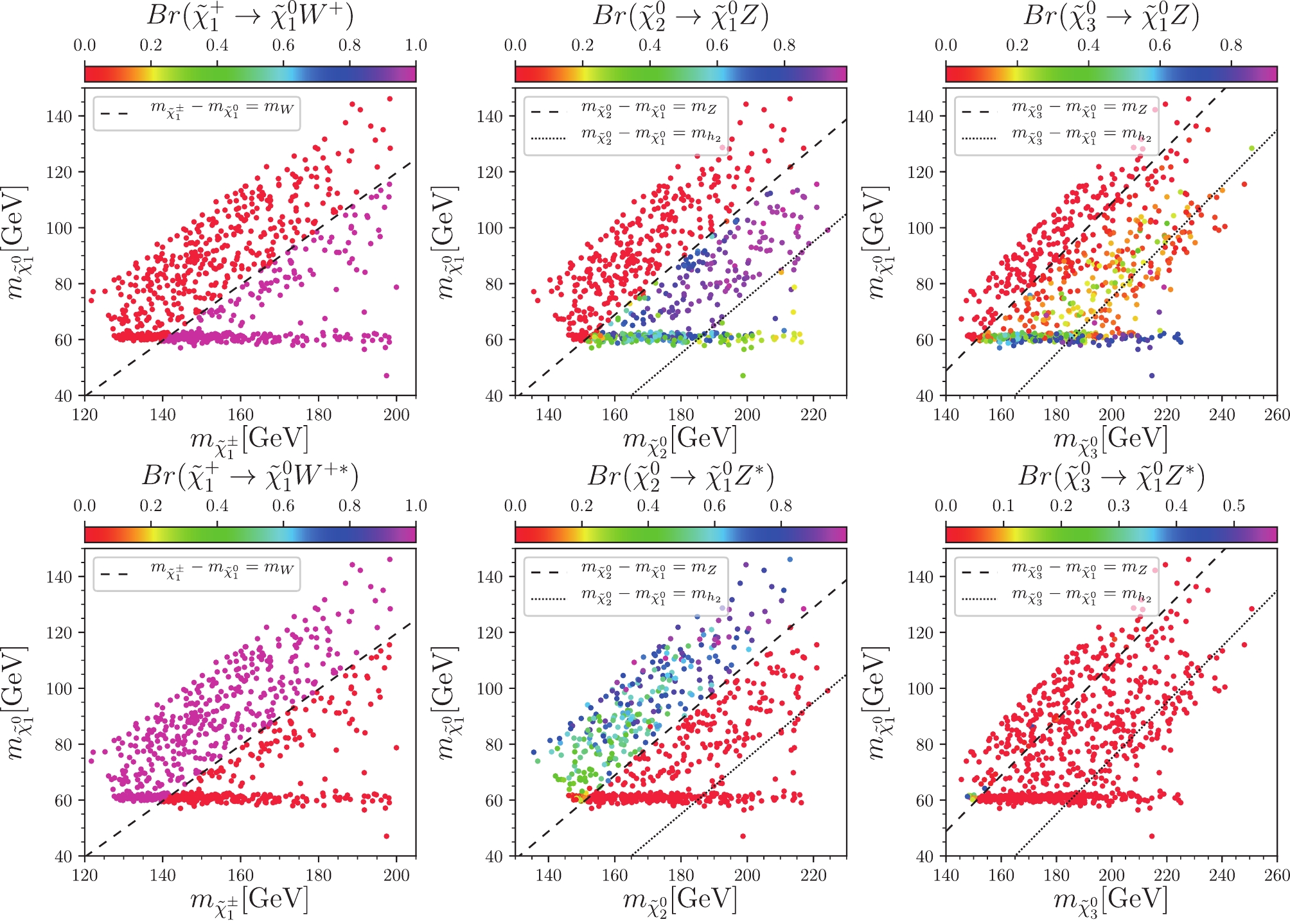

Figure 1

Figure 1.  (color online) Samples in $m_{\tilde{\chi}_1^{0}}$ versus $m_{\tilde{\chi}_i^{0}}$ planes (left $i = \pm$, middle $i = 2$, and right $i = 3$). Colors indicate branching ratios of chargino $\tilde{\chi}_1^{+}$ to $\tilde{\chi}_1^{0}$ plus W boson, and neutralino $\tilde{\chi}^0_{2,3}$ to $\tilde{\chi}_1^{0}$ plus Z boson, respectively. In the upper panel, the $W/Z$ boson is a real one, and the decay is real two-body decay; while in the lower panel the $W/Z$ boson is a virtual one and the decay is virtual three-body decay.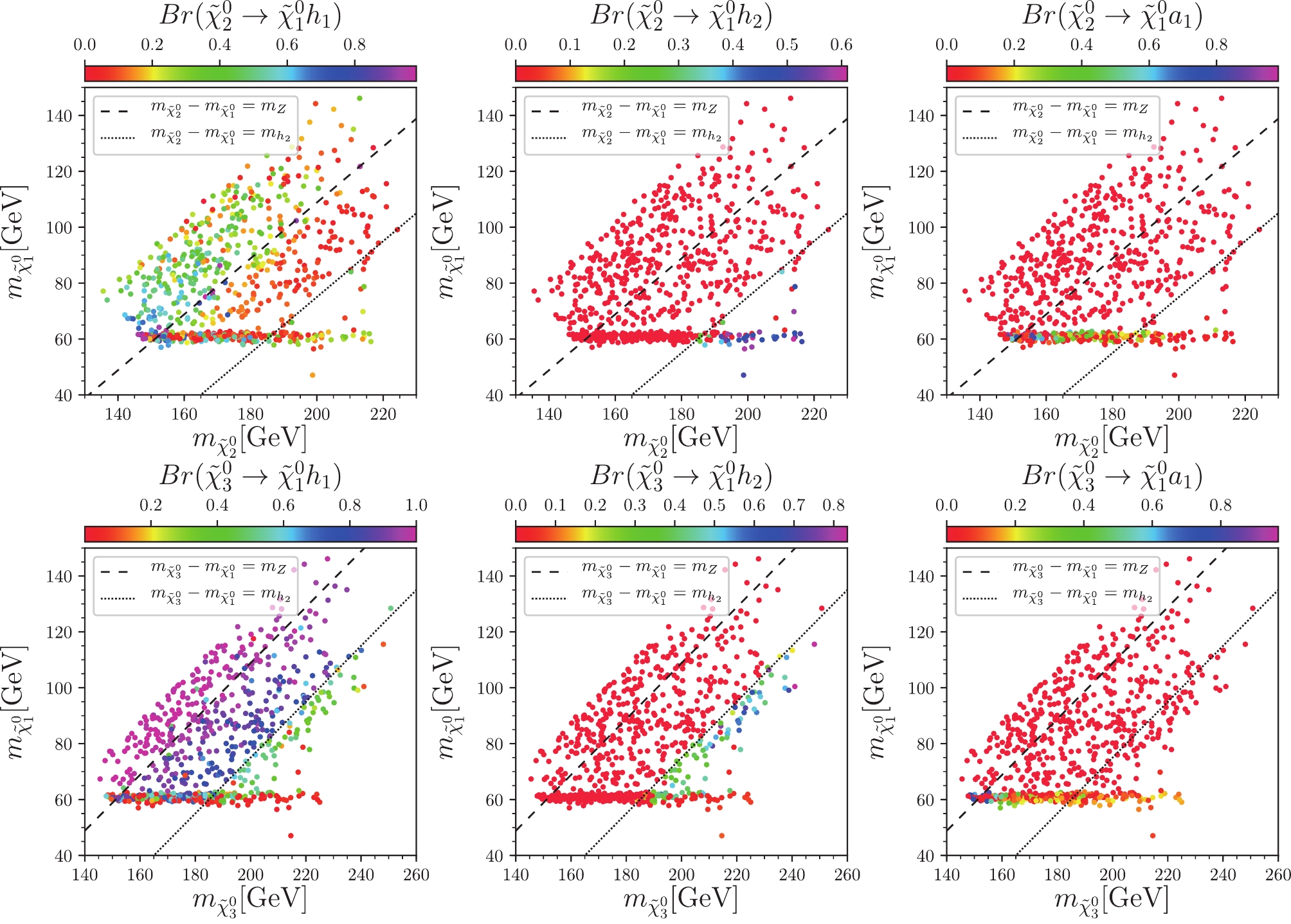

DownLoad: Full-Size Img PowerPoint

Figure 2

Figure 2.  (color online) Samples in $m_{\tilde{\chi}_1^{0}}$ versus $m_{\tilde{\chi}_i^{0}}$ planes (upper $i = 2$, lower $i = 3$). From left to the right, colors indicate the branching ratios ${\rm Br}(\tilde{\chi}_i^{0} \to \tilde{\chi}_1^{0} h_1)$, ${\rm Br}(\tilde{\chi}_i^{0} \to \tilde{\chi}_1^{0} h_2)$, and ${\rm Br}(\tilde{\chi}_i^{0} \to \tilde{\chi}_1^{0} a_1)$, respectively. The dashed and the dotted lines indicate that the mass differences, $m_{\tilde{\chi}_i^0}-m_{\tilde{\chi}_1^{0}}$, is equal to $m_Z$ and $m_{h_2}$, respectively.

DownLoad: Full-Size Img PowerPoint

The main decay modes of the neutralino $\tilde{\chi}_i^{0}$ ($i = 2,3$) are to a $\tilde{\chi}_1^{0}$ plus a Z boson or a Higgs boson. In the middle and right plots of Fig. 1 and in Fig. 2, we show the branching ratios of the neutralinos $\tilde{\chi}_i^{0}$ on the plane of $m_{\tilde{\chi}_1^{0}}$ vs $m_{\tilde{\chi}_i^{0}}$, where $i = 2,3$. In these plots, we use the dashed line, $m_{\tilde{\chi}_i^0}-m_{\tilde{\chi}_1^{0}} = m_Z$, and the dotted line, $m_{\tilde{\chi}_i^0}-m_{\tilde{\chi}_1^{0}} = m_{h_2}$, dividing the plane into three parts.

● Case I: In the region $m_{\tilde{\chi}_i^0}-m_{\tilde{\chi}_1^{0}} < m_Z$, the neutralino $\tilde{\chi}_i^{0}$ can only decay to $\tilde{\chi}_1^{0}$ plus a virtual Z boson or a light Higgs boson $h_1$. We observe from the lower middle plot of Fig. 1 and the upper left plot of Fig. 2, the $\tilde{\chi}_2^{0}$ mainly decays to a virtual Z boson plus a $\tilde{\chi}_1^{0}$, with only a small fraction to the light Higgs boson $h_1$ plus $\tilde{\chi}_1^{0}$. In contrast, the lower left plot of Fig. 2 shows that the $\tilde{\chi}_3^{0}$ mainly decays to the light Higgs boson $h_1$.

● Case II: In the region $m_Z \le m_{\tilde{\chi}_i^0}-m_{\tilde{\chi}_1^{0}} < m_{h_2}$, the neutralino $\tilde{\chi}_i^{0}$ can decay to $\tilde{\chi}_1^{0}$ plus a real Z boson or a light Higgs boson $h_1/a_1$. As shown in the upper middle plot of Fig. 1, the $\tilde{\chi}_2^{0}$ mainly decay to a real Z boson plus $\tilde{\chi}_1^{0}$. According to the upper right plot of Fig. 1 and lower left plot of Fig. 2, the $\tilde{\chi}_3^{0}$ mainly decays to a light Higgs boson $h_1$ plus $\tilde{\chi}_1^{0}$.

● Case III: In the region $m_{\tilde{\chi}_i^0}-m_{\tilde{\chi}_1^{0}} \ge m_{h_2}$, all these decay channels are opened. The $\tilde{\chi}_2^{0}$ mainly decays to $\tilde{\chi}_1^{0}$ and a 125 GeV SM-like Higgs boson $h_2$, while $\tilde{\chi}_3^{0}$ mainly decays to $\tilde{\chi}_1^{0}$ and Z bosons.

In the channel $\tilde{\chi}_i^{0} \to \tilde{\chi}_1^{0} Z$ ($i = 2,3$), like the $\tilde{\chi}_1^{\pm}\to W^\pm \tilde{\chi}_1^0$, when the mass difference is insufficient, the Z boson also becomes a virtual one. In the channel $\tilde{\chi}_i^{0} \to \tilde{\chi}_1^{0} H$ ($i = 2,3$), where the Higgs boson can be $h_1$ or $h_2$, and $h_2$ is the SM-like one. Both $h_1$ and $h_2$ mainly decay to $b \bar{b}$, thus the $t\bar{t}$ background is sizable at the LHC. In the case that Higgs decay to WW, ZZ, or ${\rm{\tau }}{\rm{\tau }}$, and W or Z decays leptonically, this might contribute to the multilepton final state. Since the light Higgs $h_1$ is highly singlet-dominated, the $\tilde{\chi}_i^{0} \to \tilde{\chi}_1^{0} h_1$ is very hard to contribute to the multilepton signal regions. Thus only the $\tilde{\chi}_i^{0} \to \tilde{\chi}_1^{0} h_2$ can visibly contribute to the multilepton signal regions.

Notably, when heavier neutralinos decay to the $\tilde{\chi}_1^{0}$ LSP, the $\tilde{\chi}_2^{0}$ and $\tilde{\chi}_3^{0}$ behave differently. Especially in the case II, $\tilde{\chi}_2^{0}$ prefers to decay to a Z boson and $\tilde{\chi}_1^{0}$, ${\rm Br}(\tilde{\chi}_2^{0} \to \tilde{\chi}_1^{0} Z) > {\rm Br}(\tilde{\chi}_2^{0} \to \tilde{\chi}_1^{0} h_1)$; while $\tilde{\chi}_3^{0}$ tends to decay to a light Higgs boson $h_1$ and $\tilde{\chi}_1^{0}$, ${\rm Br}(\tilde{\chi}_3^{0} \to \tilde{\chi}_1^{0} Z) < {\rm Br}(\tilde{\chi}_3^{0} \to$ $\tilde{\chi}_1^{0} h_1)$. The couplings $C_{h_1 \tilde{\chi}_2^{0} \tilde{\chi}_1^{0}}$ and $C_{h_1 \tilde{\chi}_3^{0} \tilde{\chi}_1^{0}}$ can be written as

where the $N_{1 1}$, $N_{1 2}$, $N_{2 1}$, $N_{2 2}$, $N_{3 1}$, and $N_{3 2}$ was set to $0$ since the wino and bino are very heavy and decoupled in the scNMSSM, and the $S_{1 1}$ and $S_{1 2}$ was set to $0$ since $|S_{1 3}|\gg |S_{1 1}|, |S_{1 2}|$. $\lambda / \sqrt{2} \ll 1$ and $\sqrt{2} \kappa \ll 1$, such that the couplings $C_{h_1 \tilde{\chi}_2^{0} \tilde{\chi}_1^{0}}$ and $C_{h_1 \tilde{\chi}_3^{0} \tilde{\chi}_1^{0}}$ are both very small and roughly the same. Meanwhile, the couplings $C_{Z \tilde{\chi}_2^{0} \tilde{\chi}_1^{0}}$ and $C_{Z \tilde{\chi}_3^{0} \tilde{\chi}_1^{0}}$ can be different from each other according to Eq. (38), which can be approximated to

where the $g_2 / c_W \sim 1$. When the two terms in Eq. (41) or Eq. (42) have different signs, and do not cancel each other, the couplings $C_{Z \tilde{\chi}_i^{0} \tilde{\chi}_1^{0}}$ can be considerably larger than $C_{h_1 \tilde{\chi}_i^{0} \tilde{\chi}_1^{0}}$; otherwise the cancel between the two terms can make $C_{Z \tilde{\chi}_i^{0} \tilde{\chi}_1^{0}}$ smaller than $C_{h_1 \tilde{\chi}_i^{0} \tilde{\chi}_1^{0}}$. For some surviving samples, $C_{Z \tilde{\chi}_3^{0} \tilde{\chi}_1^{0}}$ have the cancellation between the two terms, and that leads to small ${\rm Br}(\tilde{\chi}_3^{0} \to \tilde{\chi}_1^{0} Z)$ and large ${\rm Br}(\tilde{\chi}_3^{0} \to \tilde{\chi}_1^{0} h_1)$. Six benchmark points are listed in Table 1.

Table 1

Table 1.  Masses and branching ratios for six benchmark points in scNMSSM. Signal significance in the last line is calculated with luminosity of $300\;{\rm{fb}}^{-1}$, and with similar analysis of multi-lepton final state as in Refs. [61, 62].

	P1	P2	P3	P4	P5	P6
$m_{\tilde{\chi}_1^{\pm}}$ (GeV)	183	173	175	189	175	187
$m_{\tilde{\chi}_1^{0}}$ (GeV)	120	119	103	108	82	92
$m_{\tilde{\chi}_2^{0}}$ (GeV)	200	187	200	209	202	206
$m_{\tilde{\chi}_3^{0}}$ (GeV)	216	200	214	216	212	209
${\rm Br}(\tilde{\chi}_1^{+} \to \tilde{\chi}_1^{0} W)$	0%	0%	0%	100%	100%	100%
${\rm Br}(\tilde{\chi}_1^{+} \to \tilde{\chi}_1^{0} W^*)$	100%	100%	100%	0%	0%	0%
${\rm Br}(\tilde{\chi}_2^{0} \to \tilde{\chi}_1^{0} Z)$	0%	0%	90%	93%	94%	95%
${\rm Br}(\tilde{\chi}_2^{0} \to \tilde{\chi}_1^{0} Z^*)$	80%	65%	0%	0%	0%	0%
${\rm Br}(\tilde{\chi}_2^{0} \to \tilde{\chi}_1^{0} h_1)$	20%	35%	10%	7%	6%	5%
${\rm Br}(\tilde{\chi}_2^{0} \to \tilde{\chi}_1^{0} h_2)$	0%	0%	0%	0%	0%	0%
${\rm Br}(\tilde{\chi}_3^{0} \to \tilde{\chi}_1^{0} Z)$	1%	0%	1%	13%	13%	38%
${\rm Br}(\tilde{\chi}_3^{0} \to \tilde{\chi}_1^{0} Z^*)$	0%	0%	0%	0%	0%	0%
${\rm Br}(\tilde{\chi}_3^{0} \to \tilde{\chi}_1^{0} h_1)$	99%	100%	99%	87%	33%	62%
${\rm Br}(\tilde{\chi}_3^{0} \to \tilde{\chi}_1^{0} h_2)$	0%	0%	0%	0%	54%	0%
$ss=S/\sqrt{B} @ 300 \rm fb^{-1}$ $(\sigma)$	3.1	2.9	2.1	3.8	10.8	8.8

DownLoad: CSV

Show Table

3.3 Possibility of future discovery at HL-LHC

• 1. Introduction
• 2. Introduction to NMSSM and scNMSSM
•      2.1 Higgs sector of NMSSM and scNMSSM
•      2.2 Electroweakino sector of NMSSM and scNMSSM
• 3. Light Higgsino-dominated NLSPs in scNMSSM
•      3.1 Constraints from direct SUSY searches with CheckMATE
•      3.2 Production and decay of Higgsino-dominated NLSPs
•      3.3 Possibility of future discovery at HL-LHC
• 4. Conclusions

We investigate the possibility of future detection of electroweakinos at the HL-LHC. We adopt the same analysis of the multilepton final state by CMS [61, 62], only increasing the integrated luminosity from 35.9 ${\rm fb}^{-1}$ to 300 ${\rm fb}^{-1}$, to estimate the possibility of discovery in the future. We evaluate the signal significance by

where S and B are the number of events from signal and background processes, respectively.

In Fig. 3, we show $ss$ on the planes of $m_{\tilde{\chi}_1^{0}}$ versus $m_{\tilde{\chi}_1^{\pm}}$, $m_{\tilde{\chi}_2^{0}}$, and $m_{\tilde{\chi}_3^{0}}$ respectively. We can see that most of the samples can be evaluated at the $5\sigma$ level when the mass difference between LSP $\tilde{\chi}_1^{0}$ and NLSPs $\tilde{\chi}_1^{\pm}, \tilde{\chi}_{2,3}^{0}$ is sufficient. However, there remain some samples that cannot be checked at level above 3 or 5 sigma. The main reason is that the mass spectra is compressed, such that the leptons from the decay of NLSPs are very soft. Because ${{\not\!\!\!{\overrightarrow{p}}} _T}$ cut has to be very large at the LHC due to the large background, detecting soft particles is not easy. Combining with Figs. 1 and 2, we can learn the following facts: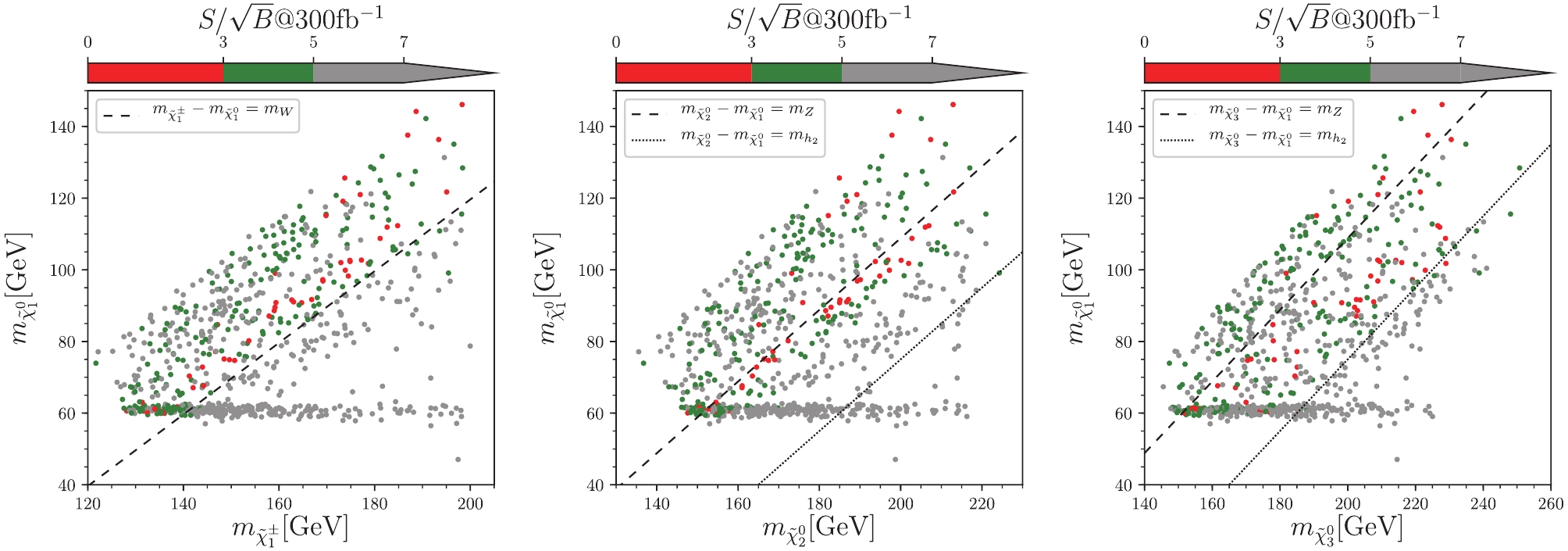

Figure 3

Figure 3.  (color online) Samples in $m_{\tilde{\chi}_1^{0}}$ versus $m_{\tilde{\chi}_1^{\pm}}$ (left), $m_{\tilde{\chi}_1^{0}}$ versus $m_{\tilde{\chi}_2^{0}}$ (middle), $m_{\tilde{\chi}_1^{0}}$ versus $m_{\tilde{\chi}_3^{0}}$ (right) planes. Colors indicate the signal significance, where red represents $ss<3\sigma$, green represents $3\sigma<ss<5\sigma$, and gray represents $ss > 5\sigma$. In the left plane, the dashed line indicates the mass difference equal to $m_W$, $m_{\tilde{\chi}_1^{\pm}}-m_{\tilde{\chi}_1^{0}} = m_W$. In the middle and right planes, the dashed line and dotted line indicate the mass difference equal to $m_Z$ and $m_{h_2}$ respectively, that is, $m_{\tilde{\chi}_i^{0}}-m_{\tilde{\chi}_1^{0}} = m_Z$ and $m_{\tilde{\chi}_i^{0}}-m_{\tilde{\chi}_1^{0}} = m_{h_2}$, where $i = 2,3$ for the middle and right planes, respectively.

DownLoad: Full-Size Img PowerPoint

● If $\tilde{\chi}_1^{\pm}$ or $\tilde{\chi}_i^{0}$ ($i = 2,3$) decays to a virtual vector boson, or in the area upon the dashed line in all the plots, the signal significance is less than $5\sigma$, and it is hard to check with $300 {\; {\rm{fb}}}^{-1}$ data at the LHC.

● If $\tilde{\chi}_1^{\pm}$ or $\tilde{\chi}_2^{0}$ decays to a real vector boson, the area between the dashed and dotted line in left and middle plots, the signal significance can be larger than $5\sigma$, which is easy to verify with $300 {\; {\rm{fb}}}^{-1}$ data at the LHC.

● The $\tilde{\chi}_3^{0}$ decay to a light Higgs $h_1$, the area between the dashed and dotted line in the right plane, the signal significance is less than $5\sigma$ for some samples. This is because the light Higgs $h_1$ mainly decay to $b\bar{b}$, which is hard to distinguish from the background.

● If $\tilde{\chi}_i^{0}$ ($i = 2,3$) decays to an SM-like Higgs, or in the area below the dotted line in middle and right plots, the signal significance is also larger than $5\sigma$ for most samples.

For the samples with insufficient mass difference between the NLSPs and LSP, the integrated luminosity 300 ${\rm fb}^{-1}$ is not sufficient. Hence, we attempted to increase the luminosity to 3000 ${\rm fb}^{-1}$, the result is that nearly all samples can be checked with $ss > 5$ at 3000 ${\rm fb}^{-1}$.

In Fig. 4, we show the signal significance $ss$ on the planes of $m_{\tilde{\chi}_1^{0}}$ versus $m_{a_1}$. We can see that there are mainly two mechanisms for dark matter annihilation: the $a_1$ funnel, where $2m_{\tilde{\chi}_1^{0}}\simeq m_{a_1}$, and the $h_2/Z$ funnel where $2m_{\tilde{\chi}_1^{0}}\simeq m_{h_2}$ or $2m_{\tilde{\chi}_1^{0}}\simeq m_{Z}$. Unfortunately, searching for the NLSPs does not contribute to distinguishing these two mechanisms. Meanwhile, as shown in Ref. [26], the spin-independent cross-section of $\tilde{\chi}^0_1$ can be sizable, such that singlino-dominated dark matter may be accessible in the future direct detections, such as XENONnT and LUX-ZEPLIN (LZ-7 2T).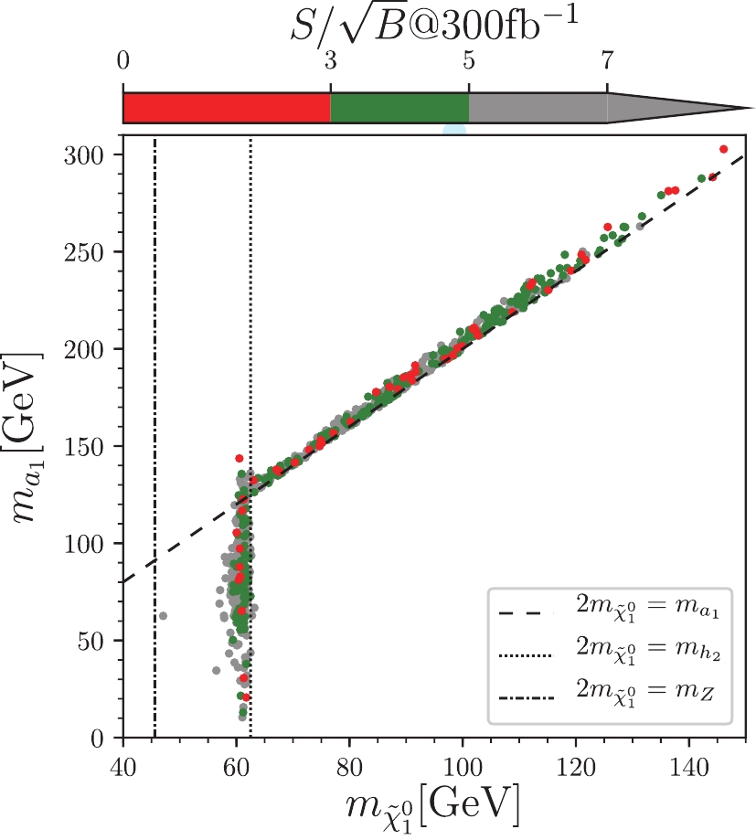

Figure 4

Figure 4.  (color online) Samples in $m_{a_1}$ versus $m_{\tilde{\chi}_1^{0}}$ plane. The color convention is the same as in Fig. 3. The dashed, dotted, and dash-dotted lines indicate $2m_{\tilde{\chi}_1^{0}}$, equal to $m_{a_1}$, $m_{h_2}$, and $m_Z$, respectively.

DownLoad: Full-Size Img PowerPoint

4. Conclusions

• 1. Introduction
• 2. Introduction to NMSSM and scNMSSM
•      2.1 Higgs sector of NMSSM and scNMSSM
•      2.2 Electroweakino sector of NMSSM and scNMSSM
• 3. Light Higgsino-dominated NLSPs in scNMSSM
•      3.1 Constraints from direct SUSY searches with CheckMATE
•      3.2 Production and decay of Higgsino-dominated NLSPs
•      3.3 Possibility of future discovery at HL-LHC
• 4. Conclusions

We discussed the light higgsino-dominated NLSPs in the scNMSSM, which is also called the non-universal Higgs mass (NUHM) version of the NMSSM. We use the scenario with singlino-dominated $\tilde{\chi}^0_1$ and SM-like $h_2$ in the scan result of our previous study on scNMSSM, where we considered the constraints including theoretical constraints of vacuum stability and the Landau pole, experimental constraints of Higgs data, muon g-2, B physics, dark matter relic density and direct searches, etc. In our scenario, the bino and wino are heavy because of the high mass bound of gluino and the unification of gaugino masses at the GUT scale. Thus, the $\tilde{\chi}^{\pm}_1$ and $\tilde{\chi}^0_{2,3}$ are higgsino-dominated and mass-degenerated NLSPs.

We first investigate the direct constraints to these light higgsino-dominated NLSPs, including searching for the SUSY particle at the LHC Run-I and Run-II. We use Monte Carlo algorithm to perform detailed simulations to impose these constraints from the search of SUSY particles at the LHC. Then, we discuss the possibility of checking the light higgsino-dominated NLSPs at the HL-LHC in the future. We use the same analysis by increasing the integrated luminosity to 300 fb⁻¹ and 3000 fb⁻¹.

Finally, we come to the following conclusions regarding the higgsino-dominated $100\sim200 \; {{\rm{GeV}}}$ NLSPs in scNMSSM:

● Among the search results for electroweakinos, the ‘multi-lepton final state’ constrains our scenario the most, and it can exclude some of our samples. Meanwhile, with all data at Run I and up to $36 {\; {\rm{fb}}}^{-1}$ data at Run II at the LHC, the search results by ATLAS and CMS still cannot exclude the light higgsino-dominated NLSPs of $100\sim200 \; {{\rm{GeV}}}$.

● When the mass difference with $\tilde{\chi}^0_{1}$ is smaller than $m_{h_2}$, $\tilde{\chi}^0_{2}$ and $\tilde{\chi}^0_{3}$ have different preferences on decaying to $Z/Z^*$ or $h_1$.

● The best channels to detect the NLSPs are though the real two-body decay $\tilde{\chi}^{\pm}_{1} \to \tilde{\chi}^0_1 W$ and $\tilde{\chi}^0_{2,3} \to \tilde{\chi}^0_1 Z/h_2$. When the mass difference is sufficient, most of the samples can be studied at the 5 $\sigma$ level with future $300 {\; {\rm{fb}}}^{-1}$ data at the LHC. For $3000 {\; {\rm{fb}}}^{-1}$ data at the LHC, nearly all of the samples can be studied at the $5\sigma$ level even if the mass difference is insufficient.

● The $a_1$ funnel and the $h_2/Z$ funnel are the two main mechanisms for the singlino-dominated LSP annihilating, which cannot be distinguished by searching for NLSPs.

We thank Yuanfang Yue, Yang Zhang, and Liangliang Shang for useful discussions.

References