The symmetry group of Feynman diagrams and consistency of the BPHZ renormalization scheme

I. INTRODUCTION

• I. INTRODUCTION
• II. SYMMETRY FACTOR AND SYMMETRY GROUP OF A FEYNMAN DIAGRAM
• III. BPHZ RENORMALIZATION SCHEME AND VERTEX OF A REDUCED FEYNMAN DIAGRAM
• IV. SYMMETRY GROUP OF A REDUCED FEYNMAN DIAGRAM $\widetilde{\Gamma}$
• V. CONTRIBUTION OF REDUCED FEYNMAN DIAGRAM $\widetilde{\Gamma}$ TO THE S MATRIX
• VI. CONCLUSION
• ACKNOWLEDGEMENTS
• APPENDIX A. Symmetry of vertex $Q_\gamma$

The principle of renormalization [1-6] in quantum field theory [7-10] is to introduce divergent counterterms in the interaction (perturbation) Hamiltonian (or Lagrangian). These terms naturally yield new terms in the S matrix [11]. They are the counterterms to eliminate the ultraviolet divergence of Feynman integrals for all Feynman diagrams to any given order [4].

Thus there are two concepts: 1. What are the counterterms in the Feynman integrals for a given Feynman diagram [12], and are they enough to give a convergent result [4]? 2. What are the counterterms in the perturbation Hamiltonian? Can they precisely give the counterterms for the Feynman diagrams to a given order? The first question was answered by the BPHZ renormalization scheme [1,4]. The second question can easily be answered for Feynman diagrams without a symmetry factor. However, for symmetric Feynman diagrams, the situation becomes more involved. To the best of our knowledge, the consistency of these two concepts would still need an explicit proof, since the non-trivial symmetry factor is an important issue in perturbation field theory [13-15].

In this paper, we study the symmetry group $G_\Gamma$ of a Feynman diagram $\Gamma$. We find that there is a subgroup $G^{(1)}_{\Gamma}$ associated with a reduced Feynman diagram $\widetilde{\Gamma}$ which keeps the union of the reduced part of $\Gamma:\bigcup_{\tau}\gamma_{\tau}$ invariant. Furthermore, the symmetry group of the reduced Feynman diagrams $\widetilde{\Gamma}$ is the quotient group $G^{(1)}_{\Gamma}/\prod_{\tau}G_{\gamma_{\tau}}$. We then explicitly give the counterterms in the perturbation Hamiltonian. We further prove that they give the counterterms of Feynman integrals for Feynman diagrams with symmetry factors. We remark that the idea of the current paper arose when the authors were editing a textbook on quantum field theory [16], and this paper is a further discussion of the material regarding the BPHZ scheme in that textbook.

The paper is organized as follows. In the next section, we introduce the symmetry group of a Feynman diagram and derive the symmetry factor appearing in the S matrix via Wick's theorem. In Section III, we review the theory of the BPHZ renormalization scheme, then give the symmetry group of $\widetilde{\Gamma}$ in Section IV. In Section V, we prove that we can consistently introduce new interaction terms (details are given in Appendix A) corresponding to each renormalization part of the Feynman diagram of a field theory, which will naturally give the counterterms required in the BPHZ scheme.

II. SYMMETRY FACTOR AND SYMMETRY GROUP OF A FEYNMAN DIAGRAM

• I. INTRODUCTION
• II. SYMMETRY FACTOR AND SYMMETRY GROUP OF A FEYNMAN DIAGRAM
• III. BPHZ RENORMALIZATION SCHEME AND VERTEX OF A REDUCED FEYNMAN DIAGRAM
• IV. SYMMETRY GROUP OF A REDUCED FEYNMAN DIAGRAM $\widetilde{\Gamma}$
• V. CONTRIBUTION OF REDUCED FEYNMAN DIAGRAM $\widetilde{\Gamma}$ TO THE S MATRIX
• VI. CONCLUSION
• ACKNOWLEDGEMENTS
• APPENDIX A. Symmetry of vertex $Q_\gamma$

The S matrix of a perturbation field theory is

Here ${\cal{H}}_I(x)$ is the perturbation Hamiltonian density, and it is a polynomial of derivatives of the fields. By Wick's theorem, the quantity

is expressed as a sum of the product of field (and derivative) contractions for all possible combinations. Each combination of a pairing of the fields corresponds to a Feynman diagram, where ${\cal{H}}_I(x)$ is related to some vertices. For each Feynman diagram, one can calculate a Feynman integral in either coordinate space or momentum space [17].

Since in a vertex of ${\cal{H}}_I(x)$ several fields may be equivalent, the corresponding vertex lines are equivalent. For definiteness, we may assign numbers to the fields, i.e. give a number to each vertex line. Changing the assignment will, in general, give a new term in the Wick's expansion. Its value is equal to the original one. In this way, for a vertex with a group of l equivalent lines in $\phi^{l}$ theory, we get a factorial $l!$. In Eq. (2), changing the assignment of $x_1\cdots x_n$ for a given contraction in Wick's expansion will give a new term in this expansion. After integrating over $x_1\cdots x_n$, these terms give the same result. In this way, we get a factorial $n!$. This means we have $n!$ equal terms, each of them corresponding to an assignment of vertices $x_i$for a Feynman diagram.

A given perturbation Hamiltonian ${\cal{H}}_{I}(x)$ may have several vertices. Each vertex is composed of a vertex point x and several vertex lines. Each of them represents a field operator. Some vertex lines of the same vertex may be equivalent (Fig. 1). Once we assign a coordinate number to a vertex point: $x = x_i$, and assign numbers $1,2,\cdots$ to each set of equivalent vertex lines (of the chosen vertex), we actually fix all of the field operators in a vertex in ${\cal{H}}_{I}(x)$ in Eqs. (1) and (2). Thus when all these vertex lines are connected pair-wise (including those in "in" and "out" states), we get a certain term in Wick's expansion. In this way, we get a Feynman diagram [12] with all vertices given coordinate numbers and all equivalent vertex lines of each vertex given line numbers.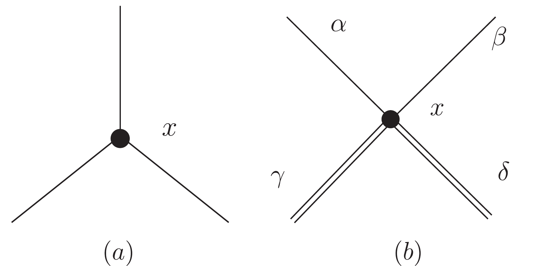

Figure 1

Figure 1.  Vertex with vertex point and vertex lines. $(a)$ Three vertex lines are equivalent. $(b)$ The two vertex lines $\alpha$ and $\beta$ are equivalent, while $\gamma$ and $\delta$ are equivalent.

DownLoad: Full-Size Img PowerPoint

Alternatively, for a blank Feynman diagram, we first assign a coordinate number ($x_1,\cdots,x_m$) to each vertex point ($p_1,\cdots,p_m$). Say, $p_1 = x_1,p_2 = x_2\cdots,p_m = x_m$. Next, for each vertex $p_a$ (and $p_b$), we assign numbers $1,2,\cdots$ to each end (attached to each vertex) of those equivalent vertex lines $L_{ab\sigma}$. Then we get a "marked" Feynman diagram, which corresponds to one term in Wick's expansion. Notice that only for topologically different "marked" Feynman diagram, we get different terms in Wick's expansion. While for different assignment of a blank Feynman diagram but topologically equivalent, they correspond to the same term in Wick's expansion (Fig. 2).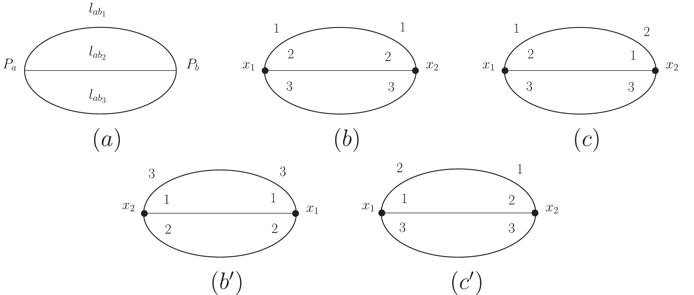

Figure 2

Figure 2.  Marking a Feynman diagram $\Gamma$. $(a)$ A blank Feynman diagram $\Gamma$ before marking. $(b)$, $(b')$, $(c)$, and $(c')$ are marked Feynman diagrams of $(a)$. $(b)$ and $(b')$ are topologically equivalent (lines $1$, $2$, and $3$ of $x_1$ connect to lines $1$, $2$, and $3$ of $x_2$, respectively). $(c)$ and $(c')$ are topologically equivalent (lines $1$, $2$, and $3$ of $x_1$ connect to lines $2$, $1$, and $3$ of $x_2$, respectively), while $(b)$ and $(c)$ are not equivalent.

DownLoad: Full-Size Img PowerPoint

The operation of marking a blank Feynman diagram can be related to a group G. Changing the assignment (marking) of a blank (unmarked) Feynman diagram can be expressed as a group element

Here $g_n$ is an element of the permutation group $S_n$, which corresponds to the reassignment of the coordinates of vertices (the permutation group is a symmetry of the Feynman diagram only after the integration over all coordinates is performed; this is also true for vertex lines). $g^i$ is an element of the symmetry group of each vertex which corresponds to the reassignment of the equivalent vertex lines of vertex point $p_i$. The operations of reassignment which do not change the topological structure of a marked Feynman diagram form a set $G_{\Gamma}$, and it satisfies the properties of a group. $G_{\Gamma}$ is the symmetry group of a blank Feynman diagram $\Gamma$.

We have $G_{\Gamma}\subset G$. For element $g_{\Gamma}\in G_{\Gamma}$, $g\in G$, and the element of G: $g' = g_{\Gamma}g$ gives a topologically equivalent marked Feynman diagram to that given by g. Thus the number of coset $m = |G|/|G_{\Gamma}|$ is the actual number of different terms in Wick's expansion which give the same blank Feynman integral form (2).

We use the following (Figs. 3 and 4) to further illustrate the action of g, $g_{\Gamma}g$, and $gg_{\Gamma}$.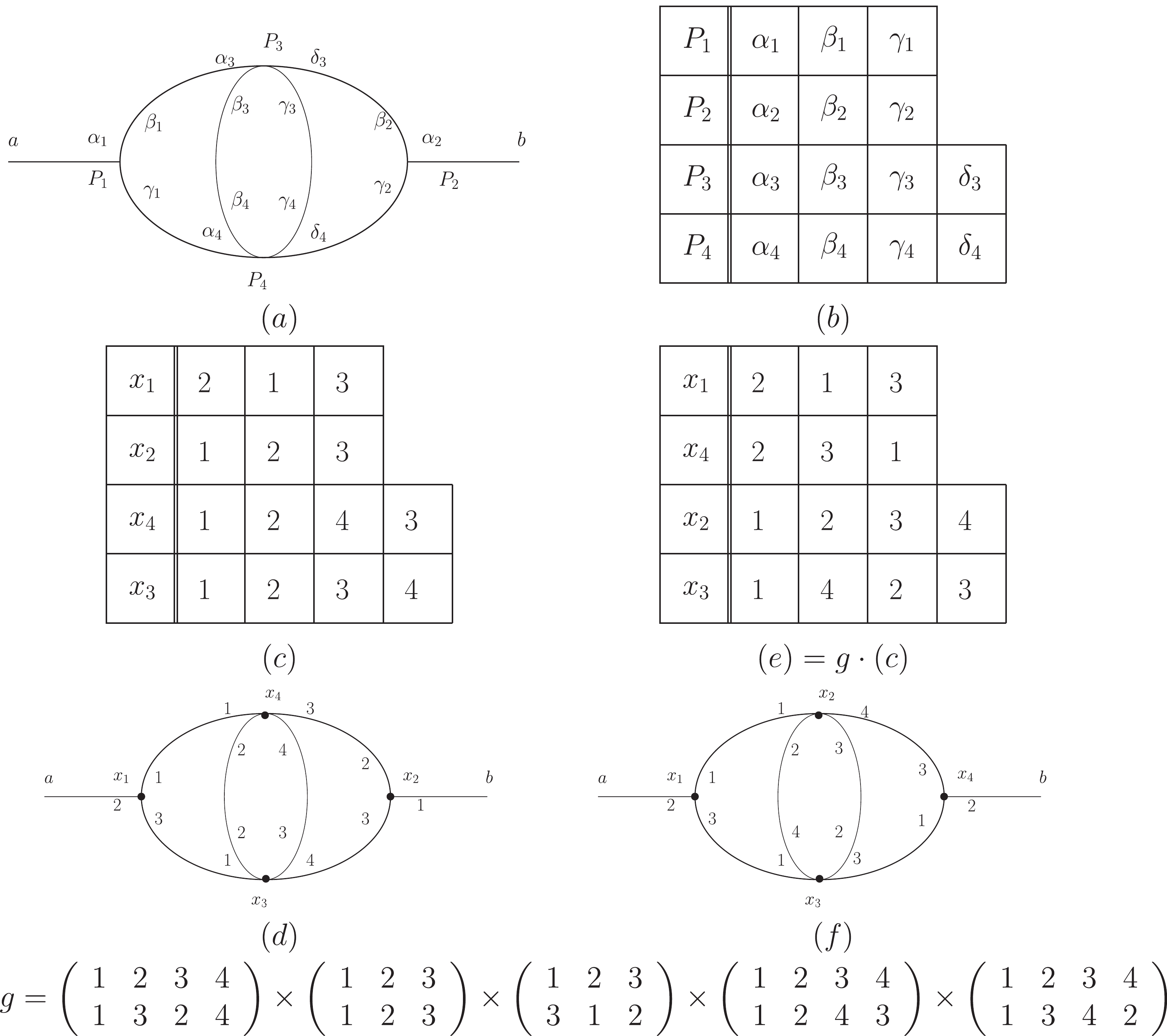

Figure 3

Figure 3.  The action of $g$ (Eq. (3)). The first factor of g acts on vertices, and the rest of factors act on attached vertex lines. $(a)$ A blank Feynman diagram. $(b)$ The vertex points ($p_1$, $p_2$, $p_3$, and $p_4)$ and vertex lines ($p_1:\alpha_1\beta_1\gamma_1$, $p_2:\alpha_2\beta_2\gamma_2$, $p_3:\alpha_3\beta_3\gamma_3\delta_3$, $p_4:\alpha_4\beta_4\gamma_4\delta_4$), where all vertex lines are equivalent for each vertex. $(c)$ An assignment of $(a)$, which gives a marked Feynman diagram $(d)$. $(e)$ Another assignment of $(a$), which gives a marked Feynman diagram $(f)$. The group element g is an operation changing the assignment, and it acts on $(d)$ giving $(f)$. The group element g acts on $(d)$, while the indices $1$, $2$, $\cdots$ in the above expression of g refer to the indices of the original blank Feynman diagram $(a)$ (and $(b)$). For example, the first factor of g swaps $P_2$ with $P_3$ in $(a)$, which means exchanging $x_2$ and $x_4$ in $(c)$ (also $(d)$). The aim of this way of labeling the Feynman diagram is to better classify different kinds of vertices and vertex lines, and to avoid confusion. This concept is in accordance with the first paragraph in Section 4.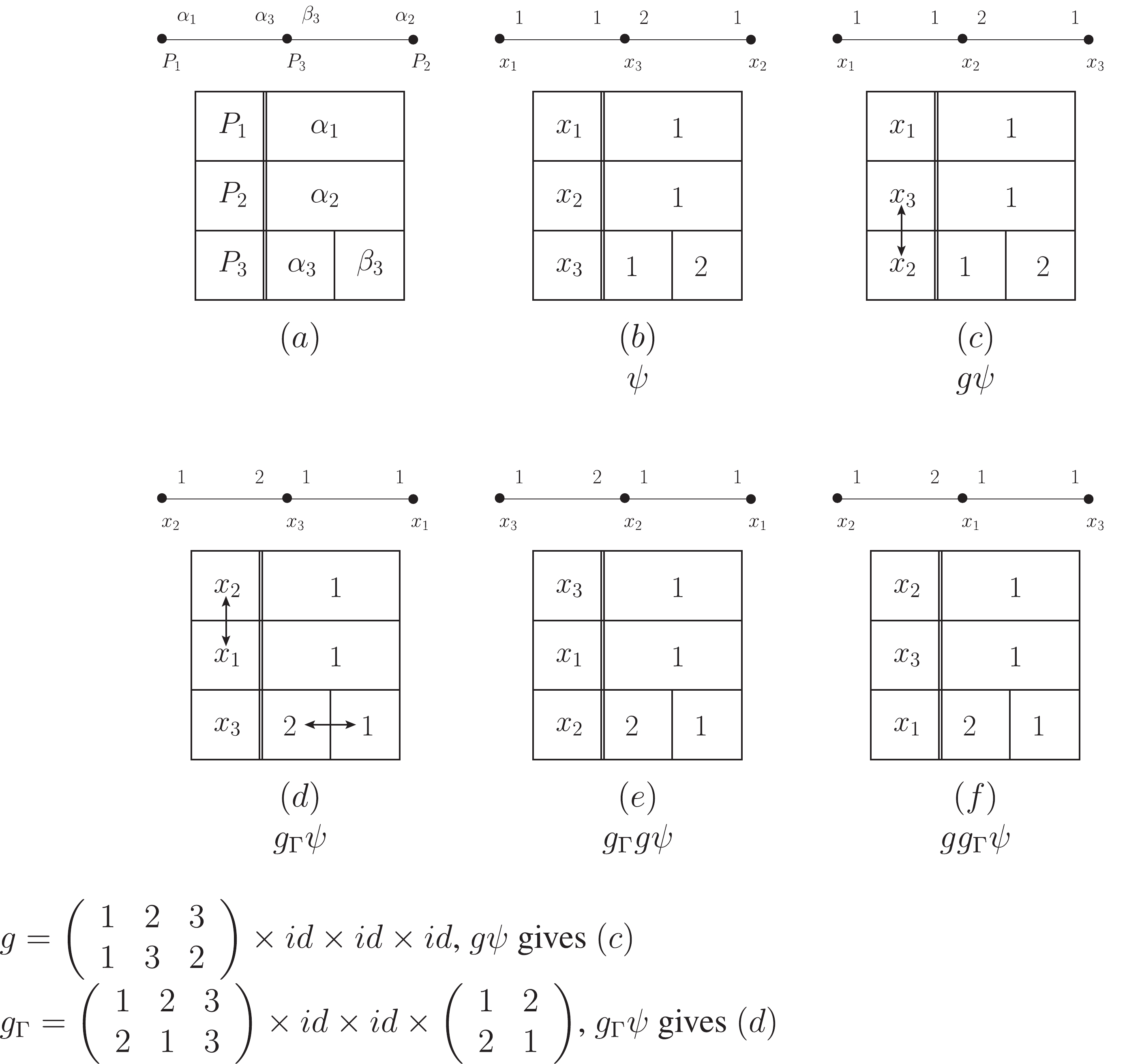

DownLoad: Full-Size Img PowerPoint

Figure 4

Figure 4.  The actions of $g_{\Gamma}g,g,$ and $gg_{\Gamma} .$ This is similar to the case in Fig. 3. Their first factors act on vertices, and the rest act on vertex lines. Similarly, the indices $1$, $2$, $\cdots$ in the above expression for g and $g_\Gamma$ refer to the indices ($P_1$, $P_2$, etc.) of the original blank Feynman diagram $(a)$. $(a)$ Blank Feynman diagram $(b)$ A marked Feynman diagram $\Gamma$ $(c)$ The action of g on $\psi$: it swaps $P_2$ with $P_3$ in $(a)$, which swaps $x_2$ with $x_3$ in $(b)$. Still $1$, $2$, and $3$ in the first factor of g correspond to $P_1$, $P_2$, and $P_3$, respectively. $(d)$ The action of $g_\Gamma$ on $\psi$: the first factor exchanges $P_1$ with $P_2$ ($x_2$ and $x_1$ in $(d)$), and the last factor exchanges vertex line $\alpha_3$ with line $\beta_3$ ($2$ and $1$ of $x_3$ in $(d)$). $(e)$ The action of $g_{\Gamma}g$ on $\psi$. Based on $(c)$, further action of $g_\Gamma$ on $g\psi$, which means swapping $x_1$ with $x_3$ in $(c)$ ($P_1$ and $P_2$ in $(a)$), and swapping $1$ with $2$ of $x_3$ in $(c)$ (vertex line $\alpha_3$ and line $\beta_3$ in $(a)$). $(f)$ The action of $gg_{\Gamma}$ on $\psi$. Based on $(d)$, further action of g on $g_{\Gamma}\psi$ means to swap $x_1$ and $x_3$ in $(d)$ ($P_2$ and $P_3$ in $(a)$). Here $(c)$ and $(e)$ are topologically equivalent, while $(c)$ and $(f)$ are topologically unequivalent. Thus $g_{\Gamma}g\psi$ and $g\psi$ correspond to the same term in Wick's expansion, but $(gg_{\Gamma})\psi$ and $g\psi$ do not.

DownLoad: Full-Size Img PowerPoint

We denote ${\cal{L}}(\Gamma)$ as the set of internal lines of $\Gamma$ and ${\cal{V}}(\Gamma)$ as the set of vertices of $\Gamma$. By Wick's expansion of Eq. (2) we get

Here $P_a$ is a numerical function depending on vertex $V_a$, and $\widetilde{\Delta}^{ab\sigma}_{F}(x_a-x_b)$ is a polynomial of derivatives of the Feynman propagator with respect to 4-coordinates $x_a$ and $x_b$. The summation is over all topologically different marked n point Feynman diagrams $\Gamma'(n)$. After integrating over all ${x_i}'s$, one obtains an integral expression in momentum space:

where $P_a$ is a polynomial of $l_{ab'\sigma'}$ (the momentum of line $L_{ab'\sigma'}$), $q_a$ is the total incoming momentum at $V_a$, while $\Delta_F$ is the Feynman propagator in momentum space. In Eq. (4) the $(-i)^n$ factor is absorbed into the $\prod P_a$ term. After integration of the momenta to eliminate $\delta$ functions, each term of connected $\Gamma'(n)$ leaves an overall $(2\pi)^{4}\delta^{4}(\Sigma q_a)$ function and an integral over independent momenta, since for the same blank Feynman diagram, integrals corresponding to different marked Feynman diagrams are equal. The contribution of the S matrix for a connected blank Feynman diagram $\Gamma(n)$ with n vertices is:

Thus one has:

The factor $(-i)$ is absorbed into each vertex of $I^0_{\Gamma}(k)$, while the term $|\prod_{i}G^{i}|$ is absorbed into each vertex of $I_{\Gamma}(k)$.

The total S matrix is then:

The second summation is over all blank Feynman diagrams with n vertices.

In Eq. (6), the momenta $k_1\cdots k_l$ are essentially those remaining after eliminating the$\delta$ functions. The set $\{k_1\cdots k_l\}$ is denoted by k.

III. BPHZ RENORMALIZATION SCHEME AND VERTEX OF A REDUCED FEYNMAN DIAGRAM

• I. INTRODUCTION
• II. SYMMETRY FACTOR AND SYMMETRY GROUP OF A FEYNMAN DIAGRAM
• III. BPHZ RENORMALIZATION SCHEME AND VERTEX OF A REDUCED FEYNMAN DIAGRAM
• IV. SYMMETRY GROUP OF A REDUCED FEYNMAN DIAGRAM $\widetilde{\Gamma}$
• V. CONTRIBUTION OF REDUCED FEYNMAN DIAGRAM $\widetilde{\Gamma}$ TO THE S MATRIX
• VI. CONCLUSION
• ACKNOWLEDGEMENTS
• APPENDIX A. Symmetry of vertex $Q_\gamma$

In the following, we deal mainly with diagrams which are connected. If we cut any internal line of a connected diagram and the diagram is still connected, we call such a diagram a proper diagram. A proper diagram $\gamma$ with superficial dimension [7-9] $d(\gamma)\geqslant0$ is called a renormalization part [4].

We have for a blank proper Feynman diagram $\Gamma$ (7):

A Feynman integral associated with a proper Feynman diagram is defined as:

where ${\cal{V}}(\Gamma)$ is the set of vertices in $\Gamma$, $q_a$ is the total incoming momentum at $V_a$, ${\cal{L}}(\Gamma)$ is the set of internal lines of $\Gamma$, and the line $L_{ab\sigma}$ is one of the lines from a vertex $V_a$ to a vertex $V_b$ with 4-momenta $l_{ab\sigma}$. The integrand $I_{\Gamma}$ is

where $\Delta_F$ is the Feynman propagator, and $P_a$ is a polynomial of $\{l_{ab\sigma}\}$ determined by the vertex of ${\cal{H}}_I(x)$.

For further derivation, we need to specify the integral parameters ${k_i}'s$. Due to the $\delta$ functions at each vertex, we have nonhomogeneous linear equations for the incoming 4-momenta $q_a$ at the vertex $V_a$,

where

is the 4-momentum on one of the lines $L_{ab \sigma}$ from the vertex $V_a$ to the vertex $V_b$. The solution is not unique for

When $\Gamma$ is connected, we define a solution for which the quantity [4]

is minimal. We call it a canonical distribution of incoming momenta $\{q_a\}$ for $\Gamma$. One can prove that $q_{ab\sigma}$ is a linear combination of ${q_a}'s$. Then generally $l_{ab\sigma}$ consists of two parts. One part comes from ${q_a}$, and the other part comes from integral variables like $k_{ab\sigma}$ (they are momenta that form inner loop flows in the connected diagram)

So here $k_{ab\sigma}$ satisfies the homogeneous linear equations (compared with Eqs. (12) and (13)):

It is important to point out that for a subdiagram $\gamma\subset\Gamma$ with a line $L_{ab\sigma}\in\gamma$ (also $L_{ab\sigma}\in\Gamma$), $q^{\gamma}_{ab\sigma}$ and $q^{\Gamma}_{ab\sigma}$ (we use the superscript to indicate the belonging) are different. From the linearity of $q_{ab\sigma}$ with respect to $q_a$, we have the following statement.

Proposition 1. The difference of $q^{\gamma}_{ab\sigma}$ and $q^{\Gamma}_{ab\sigma}$ is the canonical distribution

and thus they are linear functions of $k^{\Gamma}_{ab\sigma}$ of lines in $\Gamma$.

We can choose (not arbitrarily) some lines of $\Gamma$ to fix the parameters $k^{\Gamma}_{ab\sigma}$ and to further fix the solution. When $\Gamma$ has m loops, we can fix m lines. Then the integrals $k_1\cdots k_l$ can be chosen as $(k^{\Gamma}_{ab\sigma})^{\mu},\,\mu = 0,1,2,3$ (for $\phi^4$ theory) of these lines. For $\gamma_1,\cdots\gamma_c\subset\Gamma$ and when $\gamma_1,\cdots\gamma_c$ are disjoint diagrams, we can choose them in such a way that when the chosen lines are in $\gamma_\tau$, they also form independent lines in each $\gamma_{\tau}$. In this case, each subdiagram $\gamma_\tau$ can be reduced to a vertex. We denote the lines in the reduced diagram $\widetilde{\Gamma}$as:

Then due to proposition 1, we can properly choose independent lines such that the integral over independent momenta is:

The Feynman integral (10) is generally divergent at large k for $\Gamma$ with loops. The BPHZ renormalization scheme [7,8] gives a finite part $R_{\Gamma} = R_{\Gamma}(k,q_a)$ such that the renormalized integral converges:

Zimmermann proved the convergence of Eq. (19) [4] by an application of Weinberg's theorem [7]. The integrand $R_{\Gamma}(k,q)$ of Eq. (19) is defined by:

The sum is over all sets of renormalization parts $\gamma_{\tau}$, $\tau = 1,\cdots,c$, which are mutually disjoint. The parameters $k = \{k_1\cdots k_l\}$ are essentially the remaining momenta after integration eliminates the $\delta$ functions in Eq. (4). In Eq. (20) we have defined $I_{\Gamma/\gamma_1\cdots\gamma_\tau} = I_{\Gamma}/\prod^{c}_{\tau = 1}I_{\gamma_\tau}$, which is only determined by vertices and lines contained in $\Gamma$ but not in any $\gamma_{\tau}$. The functions $O_{\gamma}$ are recursively defined as

The sum extends over all sets of mutually disjoint renormalization parts $\{\gamma'_1,\cdots,\gamma'_{c'}\}$ (assuming they are subdiagrams of $\gamma$), but does not include $\{\gamma\}$. The function $O_\gamma$ is a Taylor series with respect to the incoming independent momentum $q^{\gamma}\equiv\{q_a\}$,

The sum of $q_j$ extends over all components of independent incoming 4-momenta of $\{q_a\}$.

Since $O_{\gamma}$ is recursively defined, one must calculate it step by step, from smaller interior renormalization parts to bigger outer ones. Due to the fact that for $\gamma'\subset\gamma$, we have proposition 1, we get:

One can conclude that $O_{\gamma}$ is a polynomial of independent components of $\{q^{\gamma}_{a}\}$. The coefficients are functions of $\{k^{\gamma}_{ab\sigma}\}$. Equation (19) can be rewritten as

where $\widetilde{J}_{\Gamma/\gamma_1\cdots\gamma_c}$ are counterterms of $J_{\Gamma}$. From Eq. (18) we have:

where $\prod\limits^{ind}$ extends to all independent lines. The integral $Q_{\gamma_\tau}$ is divergent, but it is convergent after regularization. Thus we may regard $Q_{\gamma_\tau}$ as a new vertex which corresponds to a renormalization part $\gamma_\tau$. We call it a vertex of reduction.

Equation (25) is a Feynman integral for Feynman diagram $\widetilde{\Gamma}$. It is a reduced diagram from $\Gamma$, in which all lines and vertices of $\gamma_{\tau}$ are shrunk to a vertex $\widetilde{Q}_{\gamma_\tau}$.

Can we introduce new interactions (with divergent coefficients) into interaction Lagrangian $\Delta{\cal{L}}_I$ which gives precisely these counterterms to a given order? This is a consistency problem for the BPHZ renormalization scheme. The answer is affirmative. We would like to prove this in the coming sections. It can be proved that the function $Q_{\gamma_{\tau}}$ has symmetry of $\gamma_\tau$ (Appendix A). We next study the symmetry group of $\widetilde{\Gamma}$ denoted by $G_{\widetilde{\Gamma}}$.

IV. SYMMETRY GROUP OF A REDUCED FEYNMAN DIAGRAM $\widetilde{\Gamma}$

• I. INTRODUCTION
• II. SYMMETRY FACTOR AND SYMMETRY GROUP OF A FEYNMAN DIAGRAM
• III. BPHZ RENORMALIZATION SCHEME AND VERTEX OF A REDUCED FEYNMAN DIAGRAM
• IV. SYMMETRY GROUP OF A REDUCED FEYNMAN DIAGRAM $\widetilde{\Gamma}$
• V. CONTRIBUTION OF REDUCED FEYNMAN DIAGRAM $\widetilde{\Gamma}$ TO THE S MATRIX
• VI. CONCLUSION
• ACKNOWLEDGEMENTS
• APPENDIX A. Symmetry of vertex $Q_\gamma$

In the derivation in Section II, one group element "$g^i$" in $g\in G$ for changing the number of equivalent vertex lines in a vertex is attached to a certain point $P_a$ of a blank Feynman diagram. Generally, the vertices are of different type at different points. For the symmetry group of a Feynman diagram $\Gamma$, we can alternatively attach such a group element to a running coordinate $x_j$. This is because in $g_{\Gamma}\in G_{\Gamma}$, we always have the same type of vertices for the same $x_j$ before and after reassigning. In this way, we may regard the element of $g_{\Gamma}\in G_{\Gamma}$ as a continuous mapping of a Feynman diagram into itself. This maps a vertex (including the vertex point together with all its vertex lines) into another vertex of the same type. In the following, we always refer $g_{\Gamma}$ to the second meaning.

We define a set A as the union of all ${\gamma_{\tau}}'s$

which includes all internal lines and vertex points of all ${\gamma_{\tau}}'s$. We define sets $B_{\tau}$ as all internal lines and vertex points of $\gamma_{\tau}$; actually it is $\gamma_{\tau}$ itself.

In the group $G_{\Gamma}$, those elements which do not change the set A (i.e. which map A to A) form a subgroup of $G_{\Gamma}$. We denote it as $G^{(1)}_{\Gamma}(\gamma_1\cdots\gamma_c)$. This is because the set of such elements is closed under multiplication and inversion. Similarly, we have a subgroup $G^{(2)}_{\Gamma}(\gamma_1\cdots\gamma_c) = \prod^{c}_{\tau = 1}$$G^{(2)}_{\Gamma}(\gamma_{\tau})$, where $G^{(2)}_{\Gamma}(\gamma_{\tau})\subset G_{\Gamma}$ maps each $B_{\tau} = \gamma_{\tau}$ to itself, and $G^{(2)}_{\Gamma}(\gamma_{\tau})$ keeps all lines and vertex points outside $\gamma_{\tau}$ invariant (identity). Since the mapping keeps the connection relation between the vertex points and the vertex lines of any vertex, $G^{(2)}_{\Gamma}(\gamma_{\tau})$ also keeps the "boundary points" which connect exterior lines of $\gamma_{\tau}$ invariant. We can prove that $G^{(2)}_{\Gamma}$ is a normal subgroup of $G^{(1)}_{\Gamma}$ since an element of $G^{(2)}_{\Gamma}$ does not change the exterior of A. Then we can further prove that the symmetry group of the reduced Feynman diagram $\widetilde{\Gamma}$ is the quotient group

This is because it maps the reduced vertices to themselves with their symmetry. We use (Fig. 5) to illustrate the relation between a Feynman diagram $\Gamma$ and its reduced Feynman diagrams. The configuration of $\Gamma$ with $\gamma_1\cdots\gamma_c$ can be mapped to $\Gamma$ with $\gamma_1',\cdots,\gamma_c'$ (in the same blank configuration) by each element of $G_{\Gamma}$. Those elements which keep the set A invariant form subgroup $G^{(1)}_{\Gamma}$. Let $g_{\Gamma}\in G_{\Gamma}$, and $h\in G^{(1)}_{\Gamma}$. Then for a certain $g_{\Gamma}$ and any $h\in G^{(1)}_{\Gamma}$, the element $g' = g_{\Gamma}h$ maps the set A to a set $A' = \bigcup_{\tau}\gamma_{\tau}'$. Thus the coset $G_{\Gamma}/G^{(1)}_{\Gamma}$ is characterized by different "$A'$"s which are also sets of disjoint renormalization parts of $\Gamma$. Therefore the renormalized integrand (20) can be written as: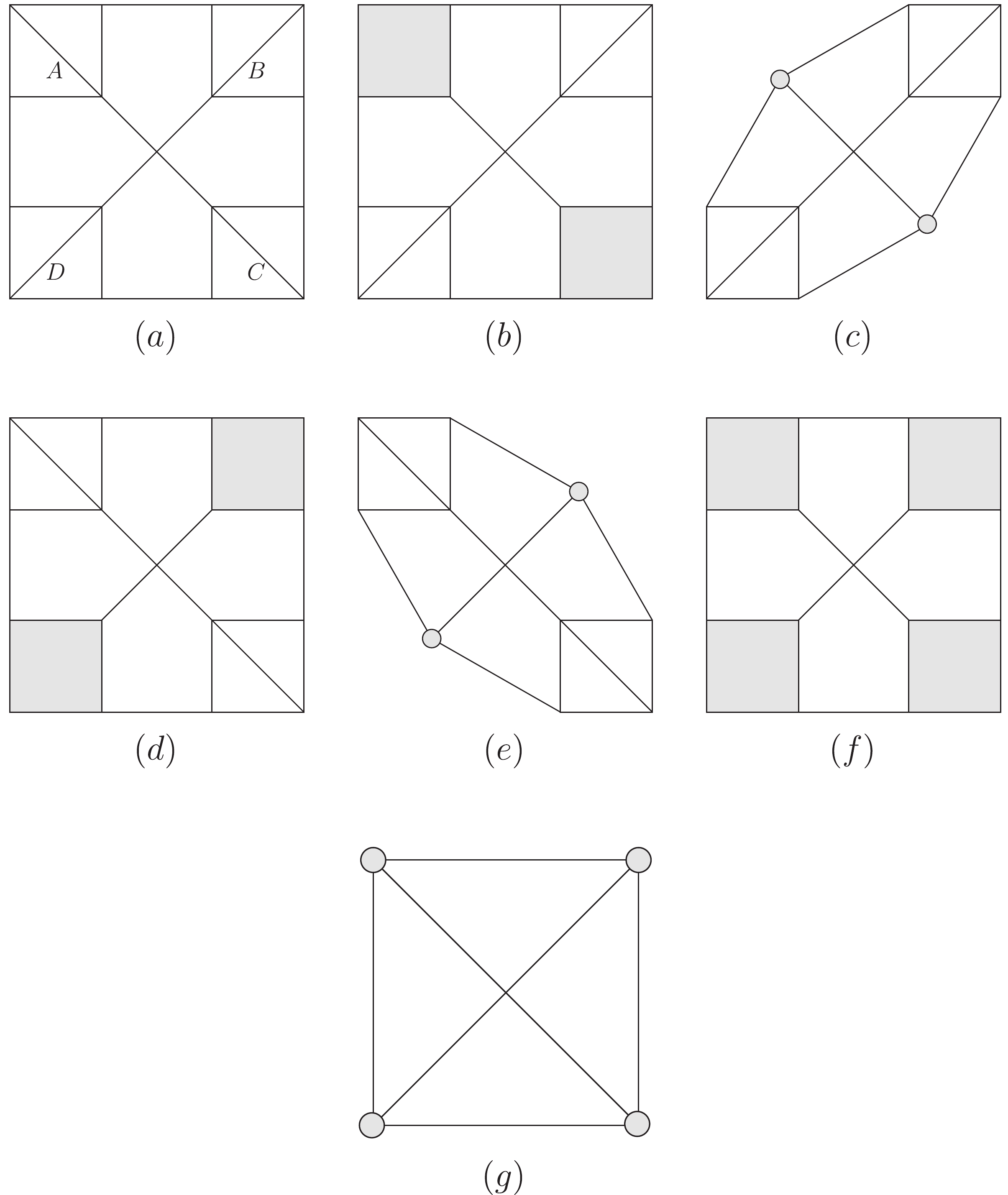

Figure 5

Figure 5.  Diagram of $\Gamma$ with $\widetilde{\Gamma}'s .$ $(a)$ Diagram of $\Gamma$ where $A,B,C,D$ are renormalization parts. $(b)$ Choose A and C as ${\gamma_{\tau}}'s$ to get $\check{\Gamma}_1$. $(c)$ $\widetilde{\Gamma}_1$ from $\check{\Gamma}_1$ (shrink all lines and points of A (and C) into a point). $(d)$ Another configuration equivalent to $(b)$, which gives $\check{\Gamma}_1'$. $(e)$ $\widetilde{\Gamma}_1'$ from $\check{\Gamma}_1'$, equivalent to $\widetilde{\Gamma}_1$. $(f)$ $\{\gamma_{\tau}\} = \{A,B,C,D\}$ gives $\check{\Gamma}_2$. $(g)$ $\widetilde{\Gamma}_2 .$

DownLoad: Full-Size Img PowerPoint

The first sum extends over all configurations of $\check{\Gamma}:\Gamma$ with different $\gamma_1\cdots\gamma_c$, which are topologically different from each other. The second sum extends over configurations produced by coset elements $G_{\Gamma}/G^{(1)}_{\Gamma}$ (acting on $\Gamma$). After integration one has the renormalized integral from Eq. (24):

where $m_{\check{\Gamma}} = \dfrac{|G_\Gamma|}{|G^{(1)}_{\Gamma}|}$. In the derivation, we need the fact that $Q_{\gamma_{\tau}}$ is symmetric under the mapping of $G_{\Gamma}$.

V. CONTRIBUTION OF REDUCED FEYNMAN DIAGRAM $\widetilde{\Gamma}$ TO THE S MATRIX

• I. INTRODUCTION
• II. SYMMETRY FACTOR AND SYMMETRY GROUP OF A FEYNMAN DIAGRAM
• III. BPHZ RENORMALIZATION SCHEME AND VERTEX OF A REDUCED FEYNMAN DIAGRAM
• IV. SYMMETRY GROUP OF A REDUCED FEYNMAN DIAGRAM $\widetilde{\Gamma}$
• V. CONTRIBUTION OF REDUCED FEYNMAN DIAGRAM $\widetilde{\Gamma}$ TO THE S MATRIX
• VI. CONCLUSION
• ACKNOWLEDGEMENTS
• APPENDIX A. Symmetry of vertex $Q_\gamma$

When we introduce new reduced vertices $\hat{Q}_{\gamma}$ to $\Delta{\cal{L}}_I = -\Delta{\cal{H}}_I$, the S matrix gets many new terms due to these new vertices. In a reduced vertex, the order of the original perturbation constant is more than one since it contains more than one original vertex. Thus if we collect terms according to the orders of original perturbation constants in the S matrix, say, n-th order, the term with respect to a reduced diagram $\widetilde{\Gamma}$ may be with a "perturbation order" m, $m<n$. We denote such a term $S_{\widetilde{\Gamma}(n,m)}$. Assume we have all reduced vertices associated with all $\gamma_{\tau}$ (renormalization part) for $n_{\gamma_\tau}\leqslant n$, and assume these vertices have the symmetry of $\gamma_\tau$. We denote the exact symmetry group for exterior lines of such vertices as $g_{O_{\gamma_\tau}}$ (see Appendix A for details). Due to the perturbation theory, there will be a term associated with $\widetilde{\Gamma}$ in the S matrix. From Eq. (6) we have:

where $G_m$ is the permutation group $S_m$, $\prod^{1}$ extends over all reduced vertices, and $\prod^{2}$ extends over the remaining original vertices in $\widetilde{\Gamma}$. Since $|G_m| = m!$, we obtain:

Together with $S_{\Gamma(n)}$, this gives:

where $\prod^{3}$ extends over all vertices in $\bigcup_{\tau}\gamma_{\tau}\subset\Gamma$. Thus one has $|\prod^{2}G^{i}|\times|\prod^{3}G^{i}| = \prod G^{i}$, which extends over all vertices of $\Gamma$. The term $S^{(n,m)}_{\widetilde{\Gamma}}$ should match the counterterms in the BPHZ renormalization scheme. We denote the vertex of $\gamma_\tau$ as $\int\prod_{ind}k^{\gamma_\tau}_{ab\sigma}O^0_{\gamma_\tau}$. Based on Eq. (25), Eq. (32) can be written as:

where $|\dfrac{G^{(2)}_{\Gamma}}{G^{(1)}_{\Gamma}}| = \dfrac{1}{|G_{\widetilde{\Gamma}}|}$, and $|\dfrac{G_{\Gamma}}{G^{(1)}_{\Gamma}}|$ is the number of cosets, which indicates the number of different $\widetilde{\Gamma}'s$ whose configurations are the same as $\widetilde{\Gamma}$.

Taking into account all reduced diagrams of $\Gamma$, we have:

where l is specified by the set $\{\gamma_1\cdots\gamma_c\}$ of mutually disjoint renormalization parts in $\Gamma$.

Next we absorb all factors $|G^{i}|$ of symmetry groups of the original vertices into these vertex constants, and require

which corresponds to $O^0_{\gamma_\tau}$ in Eq. (34). We have:

This is just the BPHZ formula. The corresponding operator of $\hat{O}^0_{\gamma_\tau}$ in Eq. (35) is given in Appendix A, and it only depends on the renormalization part $\gamma_{\tau}$.

VI. CONCLUSION

• I. INTRODUCTION
• II. SYMMETRY FACTOR AND SYMMETRY GROUP OF A FEYNMAN DIAGRAM
• III. BPHZ RENORMALIZATION SCHEME AND VERTEX OF A REDUCED FEYNMAN DIAGRAM
• IV. SYMMETRY GROUP OF A REDUCED FEYNMAN DIAGRAM $\widetilde{\Gamma}$
• V. CONTRIBUTION OF REDUCED FEYNMAN DIAGRAM $\widetilde{\Gamma}$ TO THE S MATRIX
• VI. CONCLUSION
• ACKNOWLEDGEMENTS
• APPENDIX A. Symmetry of vertex $Q_\gamma$

In conclusion, we have considered the procedure for introducing a new vertex $\hat{Q}^0_{\gamma_\tau}$ into $\Delta{\cal{L}}_I$ for all renormalization parts $\gamma_\tau$ (proper diagram with $d(\gamma_\tau)\geqslant0$) with number of vertices $m\leqslant n$. When we collect all terms of original parameter order $m'\leqslant n$ (the order for original perturbation parameters) in the S matrix, then it will automatically give the counterterms of Feynman integrals as the BPHZ scheme requires for any Feynman diagram $\Gamma$.

Thus the BPHZ scheme is consistent with adding counterterms in $\Delta{\cal{L}}_{I}$.

ACKNOWLEDGEMENTS

• I. INTRODUCTION
• II. SYMMETRY FACTOR AND SYMMETRY GROUP OF A FEYNMAN DIAGRAM
• III. BPHZ RENORMALIZATION SCHEME AND VERTEX OF A REDUCED FEYNMAN DIAGRAM
• IV. SYMMETRY GROUP OF A REDUCED FEYNMAN DIAGRAM $\widetilde{\Gamma}$
• V. CONTRIBUTION OF REDUCED FEYNMAN DIAGRAM $\widetilde{\Gamma}$ TO THE S MATRIX
• VI. CONCLUSION
• ACKNOWLEDGEMENTS
• APPENDIX A. Symmetry of vertex $Q_\gamma$

All Feynman diagrams in this paper were drawn by the program JaxoDraw [18]

APPENDIX A. Symmetry of vertex $Q_\gamma$

• I. INTRODUCTION
• II. SYMMETRY FACTOR AND SYMMETRY GROUP OF A FEYNMAN DIAGRAM
• III. BPHZ RENORMALIZATION SCHEME AND VERTEX OF A REDUCED FEYNMAN DIAGRAM
• IV. SYMMETRY GROUP OF A REDUCED FEYNMAN DIAGRAM $\widetilde{\Gamma}$
• V. CONTRIBUTION OF REDUCED FEYNMAN DIAGRAM $\widetilde{\Gamma}$ TO THE S MATRIX
• VI. CONCLUSION
• ACKNOWLEDGEMENTS
• APPENDIX A. Symmetry of vertex $Q_\gamma$

Similar to $G_\Gamma$, we define a mapping group $G_{\hat{\gamma}}$ for the Feynman diagram $\gamma$. In this mapping, we allow the external lines to be mapped to equivalent lines of another vertex of the same type. This is different from $G_\Gamma$, where the external lines always keep fixed. We find that the group $G_\gamma$ is a normal subgroup of $G_{\hat{\gamma}}$. We denote $\hat{\gamma}$ with external lines of $\gamma$ belonging to ${\cal{L}}(\hat{\gamma})$. We have:

and

due to Eq. (25). Assume for all proper renormalization parts $\gamma_{\tau}\subset\gamma$, $O_{\gamma_{\tau}}$are symmetric functions with the symmetry of $\gamma_{\tau}$. That means, under $G_{\hat{\gamma}_{\tau}}$, the value of $Q_{\gamma_{\tau}}$ is invariant. We can write Eq. (A2) as:

Here $V_{\gamma}$ is defined as:

in which:

The situation is similar for $\check{I}_{\gamma/\{\gamma_1\cdots\gamma_c\}}$, and Eq. (A4) is invariant under the mapping of $G_{\hat{\gamma}}$. Thus we can always choose $V_{\gamma}(s)$ which is invariant under $G_{\hat{\gamma}}$. On the other hand, we can also choose $V_{\gamma}(ind)$ which is only a function of independent $q^{\gamma}_a$. Due to $\delta^4(\sum^a q_a)$ in Eq. (A4), the number of independent ${q_{a}^{\gamma}}$ is less than the number of all ${q_{a}^{\gamma}}$. We have:

One can show by truncating the Taylor series in Eq. (22) that:

where $-t^{\gamma}(ind)V_{\gamma}(ind)$ is the $Q_\gamma$ in Eq. (A2). We then prove that $Q_\gamma$ can also be chosen as a symmetric (invariant) function under the mapping of $G_{\hat{\gamma}}$. It is fixed under $G_\gamma$. Thus as a reduced vertex, we have the symmetry group,

Here we make a remark about invariants. If the momenta of external lines change following the mapping, the function $Q_{\gamma}$ is invariant. For example, under the mapping depicted in Fig. A1, if the function $f(x_1, x_2,x_3) =$ $f(x_1', x_2',x_3')$, we say function f is invariant under the mapping g.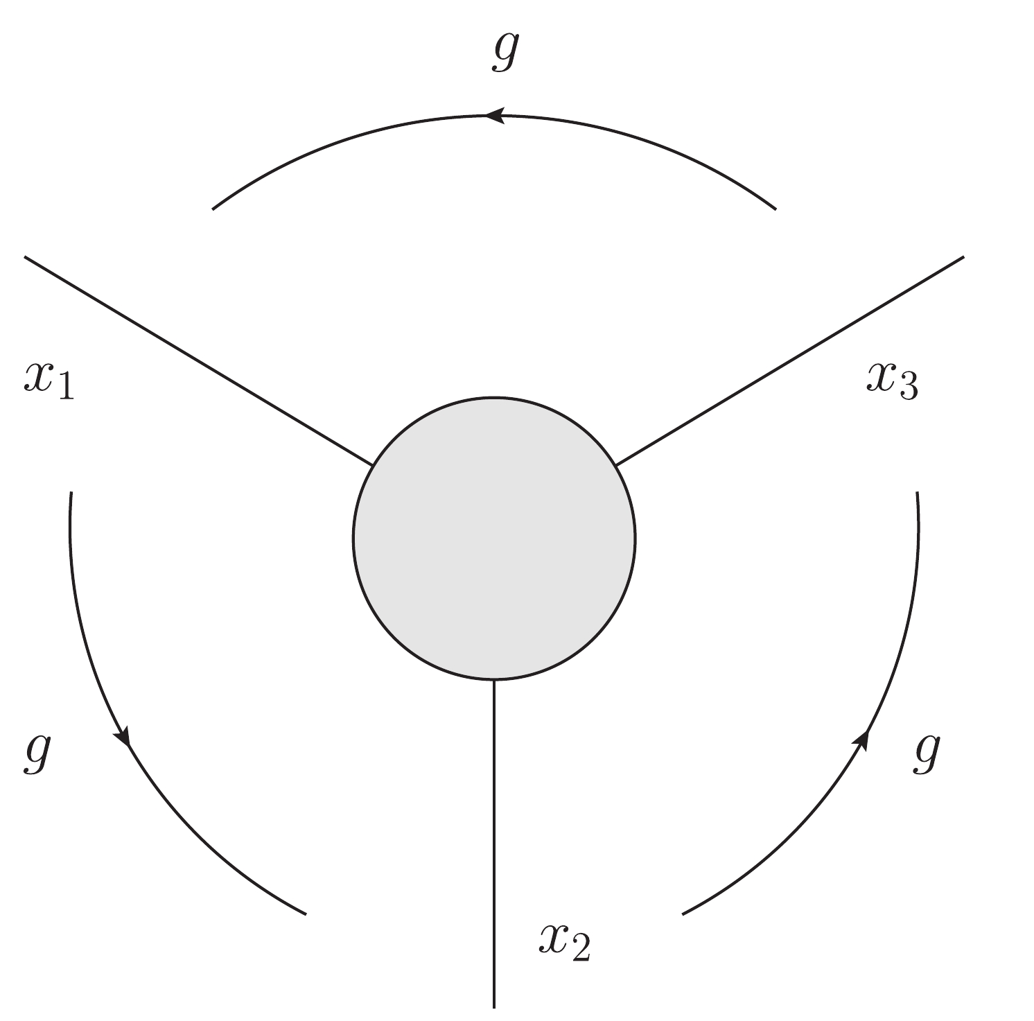

Figure A1

Figure A1.  Mapping leading to an invariant function ($x_1'=x_2, x_2'=x_3,x_3'=x_1$).

DownLoad: Full-Size Img PowerPoint

We denote $Q_{\gamma}$ as

In the integral equations (1) and (2), the derivative $\left(-{\rm i}\dfrac{\partial}{\partial x_a}\right)$ operator produces a momentum $q_a$ factor. Thus the function $Q_\gamma$ can be realized in $\Delta{\cal{L}}_I$ by the operator proportional to

where $i_1,\cdots,i_l$ in summation run over all $a = 1,\cdots,n_{\gamma}$, $(n_\gamma = \text{number of vertices in }\gamma)$, and $\mu = 0,1,2,3.$ In Eq. (A10), fields $\{\varphi_{a_i},i = 1,\cdots,l_a\}$ produce external lines at the vertex $V_a,\cdots$.

From Eq. (35) the operator of the reduced vertex introduced in $\Delta{\cal{L}}_I$ is then

$G_{{\gamma}_\tau}$ is a normal subgroup of $G_{\hat{\gamma}_\tau}$, see Fig. A2 below.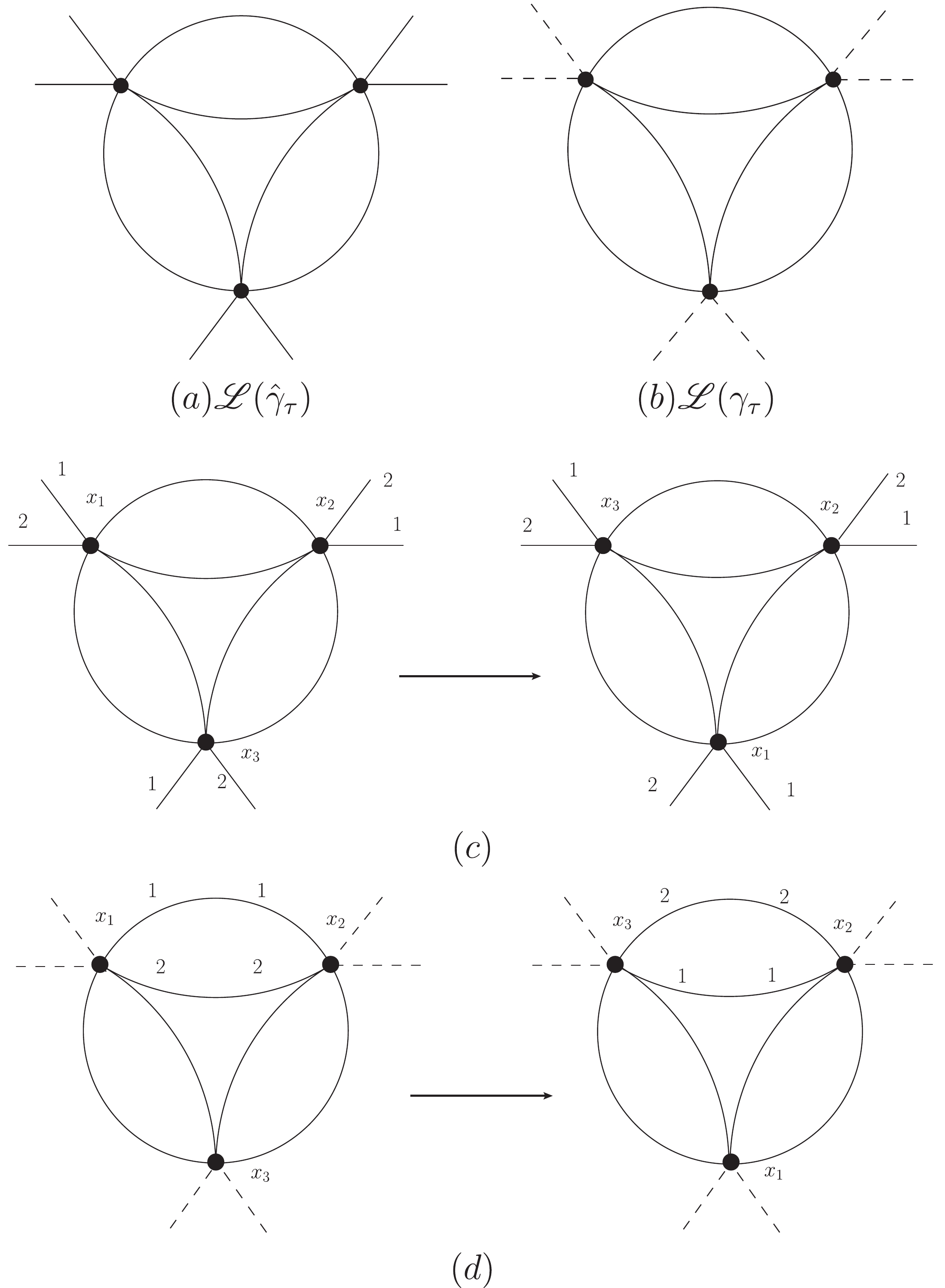

Figure A2

Figure A2.  A renormalization part $\gamma_\tau$ and associated $G_{\hat{\gamma}_\tau}$ and $G_{{\gamma}_\tau}$. $(a)$ The lines belonging to $\hat{\gamma}_\tau$. $(b)$ The lines (only internal lines!) belonging to $\gamma_{\tau}$. $(c)$ A mapping $g_{\hat{\gamma}_\tau}$, including the change of points and external lines of $\gamma_\tau$. This mapping does not belong to $G_{\gamma_\tau}$. $(d)$ A mapping $g_{\gamma_{\tau}}\in G_{\gamma_{\tau}}\subset G_{\hat{\gamma}_{\tau}}$.

DownLoad: Full-Size Img PowerPoint

References