Processing math: 1%

U(1)Lμ-Lτ breaking phase transition, muon g–2, dark matter, collider, and gravitational wave

  • Combining the dark matter and muon g2 anomaly, we study the U(1)LμLτ breaking phase transition, gravitational wave spectra, and direct detection at the LHC in an extra U(1)LμLτ gauge symmetry extension of the standard model. The new fields include vector-like leptons (E1,E2,N), the U(1)LμLτbreaking scalar S, and the gauge boson Z, as well as the dark matter candidate XI and its heavy partner XR. A joint explanation of the dark matter relic density and muon g2 anomaly excludes the region where both min and \min(m_{Z'},m_S) are much larger than m_{X_I} . In the parameter space accommodating the DM relic density and muon g-2 anomaly, the model can achieve a first-order U(1)_{L_\mu-L_\tau} breaking phase transition, whose strength is sensitive to the parameters of the Higgs potential. The corresponding gravitational wave spectra can reach the sensitivity of U-DECIGO. In addition, the direct searches at the LHC impose stringent bounds on the mass spectra of the vector-like leptons and dark matter.
      PCAS:
    • 04.60.Bc(Phenomenology of quantum gravity)
  • Recently, the Event Horizon Telescope (EHT) Collaboration presented images of black holes at the center of the Messier 87^{*} ({\rm{M}} 87^{*} ) galaxy and the Milky Way [15]. These images observed by the EHT are an important validation of general relativity (GR) and share a common feature that always presented as a black disk surrounded by a bright ring. Owing to the strong gravity of a black hole, photons may travel around it many times and then escape to the screen of the observer, leading to a bright ring. The black disk represents the region in which the photons are fully absorbed by the black hole, which is known as the black hole shadow.

    The shadows of different types of black holes have been theoretically investigated in recent years. Synge was the first to discover that the shadow contour of a black hole is a standard circle [6]. For a rotating black hole, the shadow deforms in the direction of rotation and has a D-shape [7, 8]. Considering that there is always a significant amount of accretion matter around black holes in the universe, the spectrum of the accretion disk around a Kerr black hole was investigated but not plotted [9]. Subsequently, the image of the accretion disk was obtained from a physical model of the thin gas disk surrounding a Schwarzschild black hole, and the appearance of the shadow and photon ring was found to be related to accretion radiation [10]. Although the intensity depends on the details of accretion flow, its outline is only determined by the spacetime itself and corresponds to the apparent shape of photon orbits captured by the observer. By considering spherically symmetric accretion, the shadow of a Schwarzschild black hole has also been explored [11]. Based on the optical and geometrically thin disk around a Schwarzschild black hole, Gralla et al. made the groundbreaking discovery that black holes not only have photon and lensing rings, but also direct emission [12]. Since then, many related studies on different accretion models have been continuously conducted [1336].

    Interestingly, a thin-shell wormhole (TSW), another special object in our universe, is a topological structure that connects two spacetimes through a throat, which was originally indicated by Misner and Wheeler [37]. Morris and Thorne were the first to propose the concept of a traversable wormhole and showed that exotic matter can be present in its throat [38]. A wormhole produced by surgically grafting two Schwarzschild spacetimes allows a traveler to avoid regions of exotic matter while traveling through the wormhole without experiencing any forces, tides, or other disturbances [39, 40]. These types of wormholes are simple and allow for the minimization of violations of the null energy condition while enabling partial dynamical stability analysis and further constraints on the equation of state of exotic matter. Exploring the stability of wormhole models is important in determining whether a wormhole is traversable. In Ref. [41], Poisson and Visser investigated the stability of a TSW under linear perturbations. Subsequent studies extended this work to more general cases [42], and nonlinear situations have also attracted considerable attention [4346]. More importantly, it is generally believed that the exploration of the light ring and shadow of a wormhole can help further understand the structure of wormholes. The formation of a Schwarzschild TSW shadow is closely related to the position of the light source and observer [47]. For a Reissner-Nordstrom asymmetric thin-shell wormhole (ATSW), Wielgus et al. discovered that the image seen by the observer may contain a photon ring on the observer's side and a photon ring on the other side of the wormhole [48]. In the framework of Palatini f(R) gravity, it is possible to observe double shadows [49]. Considering the ATSW model, the impact parameter of null geodesics in a wormhole is generally discontinuous, and a novel shadow appears in three cases. In one case, the size of the shadow depends on the size of the photon sphere on the other side of the spacetime and is relatively small compared to that of the black hole case [50]. The novel ATSW shadow structure observed when there was an accretion disk in the observer's spacetime was previously explored, which was found to be noticeably different from that in the black hole case [51].

    The problem with GR is that there is a singularity in the spacetime where the curvature becomes infinite. Quantum gravity theory may be regarded as a perfect candidate to circumvent this problem. At present, a self-consistent quantum gravity theory is lacking. Therefore, many theories that correct gravity or quantum mechanics have emerged to provide extensive insight into quantum gravity. For example, Bonanno and Reuter used the renormalization group method to obtain a class of Schwarzschild black holes renormalized by considering a type of nonlinear transformation group in classical mechanics [52, 53]. These black holes can terminate Hawking's evaporation process before reaching the critical mass, replacing the singularity with a smooth de Sitter core to avoid exposing the singularity, which is consistent with the cosmic censorship hypothesis [53]. In such black holes, there are two parameters, Ω and γ, which originate from non-perturbative renormalization group theory and an identification of distance scale cutoff, respectively [53, 54]. In [53, 54], the curvature at the center of black hole avoids the singularity perfectly owing to the existence of Ω and γ. Thus, it is clear that a renormalization group improved (RGI) black hole can present the effect of quantum gravity via Ω and γ. Using this black hole, we studied the shadow characteristics of an RGI black hole surrounded by spherical accretion models and found the effect of quantum gravity on the shadow appearance [17]. In addition, many other studies related to this black hole have been conducted, as referenced in [5456]. Using Visser's method, the spacetime with RGI terms can also be cut and pasted as an ATSW, which would exhibit more features of parameters Ω and γ. To further explore the feature of quantum gravity, considering a thin disk on one side of an ATSW, we study the observable appearance of an ATSW encoded with the RGI spacetime on two sides. In particular, when photons are emitted from the thin disk, some with a certain impact parameter approach the throat but do not fall into it. However, some photons fall into the throat and then turn back owing to the asymmetric structure, eventually reaching infinity. Considering this, we carefully study the trajectories of photons and investigate the novel light rings of the RGI-ATSW. Furthermore, the effects of the RGI parameters on the observable appearance of the ATSW are addressed throughout the study.

    The structure of this paper is as follows. In Sec. II, the ATSW system with RGI terms is introduced and its geodesics are briefly studied. We investigate the light deflection of wormhole and analyze the photon trajectories in Sec. III, and the transfer function of the ATSW when a thin accretion disk is located on one side of the spacetime, i.e., M_{1} , and obtain its optical appearance using two different radiation scenarios for the disk in Sec. IV. Additionally, we compare the appearance of the RGI-ATSW with those of a Schwarzschild-ATSW and an RGI black hole. Finally, in Sec. V, we present our conclusions.

    Using the well-known cut and paste approach provided by Visser, it is easy to construct an ATSW structure in which the two spacetimes are joined by the throat [39], where the different mass parameters in the two spacetimes reflect the asymmetric structure of the TSW. In [53], the well-known RGI black hole solution was obtained, which can be represented as

    {\rm d} s^2 = -F (r) {\rm d} t^2+ F(r)^{-1} {\rm d} r^2+r^2 {\rm d} \theta ^2 +r^2 {\sin^2\theta} {\rm d} \varphi^2,

    (1)

    with F(r) = 1-\dfrac{2M}{r} \left( 1+\dfrac{\Omega M^{2}}{r^{2}}+\dfrac{\gamma \Omega M^{3}}{r^{3}} \right) ^{-1} , where M represents the black hole mass, and γ and Ω are dimensionless parameters obtained by distance scale intercept identification and non-perturbative renormalization group theory, respectively [53, 54]. When F(r) = 0 , there are two roots, representing the inner and outer horizons of the black hole. The outer horizon is commonly referred to as the event horizon, denoted by r_+ . According to Visser's method, spacetime structure (1) out of the horizon can be used to construct an ATSW. In general, the profile of a wormhole can be viewed as Fig. 1. The two spacetimes with different mass parameters are defined as M_{1} and M_{2} , which are joined through a thin-shell to form a new manifold, M\equiv M_{1} \cup M_{2} . In this case, the spacetimes and throat produce an ATSW with different mass parameters. Therefore, when the two spacetimes out of the throat are regarded as (1), the metric can be rewritten as

    Figure 1

    Figure 1.  Profile of a wormhole, in which two spacetimes are connected by a throat.

    {\rm d} s_{i}^2 = -F_{i} (r_{i}) {\rm d} t_{i}^2+ F_{i}(r_{i})^{-1} {\rm d} r_{i}^2+r_{i}^2 {\rm d} \theta_{i} ^2 +r_{i}^2 {\sin^2\theta_{i}} {\rm d} \varphi_{i}^2,

    (2)

    where i = 1,2 , and

    F_{i}(r_{i}) = 1-\dfrac{2M_{i}}{r_{i}} \left( 1+\dfrac{\Omega M_{i}^{2}}{r_{i}^{2}}+\dfrac{\gamma \Omega M_{i}^{3}}{r_{i}^{3}} \right) ^{-1},\quad r\geq R,

    (3)

    where R represents the radius of the throat. Here, we consider R to be greater than the event horizon of spacetime (1); hence, it satisfies R> \max\left\{ r_{1_{+}}, r_{2_{+} } \right\} . The \dot R denotes the 4-velocity of the thin-shell. For simplicity, we assume the thin-shell wormhole to be static, i.e., \dot R = 0 .

    First, we focus on the motion of photons in the RGI-ATSW model. For simplicity, we fix the photons on the equatorial plane and assume that there is only a gravitational interaction between photons and the throat and that the 4-momentum of the photons remains constant during the pass through the wormhole. Additionally, we consider continuity of the metric in spacetime M, i.e., g_{ab}^{M_{1}}(R) = g_{ab}^{M_{2}}(R) [50]. The energy E and angular momentum L are conserved along the geodesics:

    E_{i} = -p_{t_{i}}, \quad L_{i} = p_{\varphi_{i}}.

    (4)

    Therefore, the motion equation of null geodesics can be written as

    \dfrac{(p_{i}^{r_{i}})^{2}}{F_{i}(r_{i})} = \dfrac{p_{t_{i}}^{2}}{F_{i}(r_{i})}-\dfrac{p_{\varphi_{i}}^{2}}{r_{i}^{2}},

    (5)

    where p^{a} is the 4-momentum of the massless particles along the geodesic, p^{a} = \dfrac{{\rm d} x^{\mu}}{{\rm d} \lambda}, and λ is an affine parameter. The affine parameter λ can be redefined as \lambda = \lambda/E , and b = |L|/E is the impact parameter. Therefore, Eq.(5) can be rewritten as

    (p_{i}^{r_{i}})^{2} = \dfrac{1}{b_{i}^{2}}-\dfrac{F_{i}(r_{i})}{r_{i}^{2}}.

    (6)

    Here, the effective potential V_{\rm eff}(r_{i})is introduced,

    V_{\rm eff}(r_{i}) = \dfrac{F_{i}(r_{i})}{r_{i}^{2}}.

    (7)

    The photon sphere condition requires V_{\rm eff}(r_{p}) = \dfrac{1}{b_{c}^{2}} and V'_{\rm eff}(r_{p}) = 0, where r_{p} is the radius of the photon sphere, and b_{c} represents the corresponding critical impact parameter. The effective potential of the RGI-ATSW is shown in Fig. 2, which is

    Figure 2

    Figure 2.  (color online) Effective potential of the RGI-ATSW, where the dashed and solid lines represent spacetimes M_1 and M_2 , and M_1 = 1 , M_2 = 1.2 , R = 2.6 . For \Omega = 0.1 and \gamma = 0.1 , the impact parameter b_{c1} \approx 5.13527 and A \cdot b_{c2} \approx 3.89905 .

    According to Fig. 2, the effective potentials of the two spacetimes are equal at the throat, and the maximum effective potential in spacetime M_2 is greater than that in M_1 . Taking \Omega = 0.1 and \gamma = 0.1 as an example, the effective potentials can be classified into three cases. Case 1 (Region 1): The photon with impact parameter b_1>5.13527 from M_1 is reflected by the potential barrier of M_1 when it is close to the throat and then reaches the infinity of M_1 . Case 2 (Region 2): The photon with impact parameter 3.89905<b_1<5.13527 falls into the throat and then reaches the spacetime M_2 through the throat but is reflected back to M_1 by the potential barrier of M_2 , finally reaching infinity in M_1 . Case 3 (Region 3): The photon with impact parameter b_1<3.89905 falls into the throat and enters the spacetime M_2 , and eventually, it no longer returns to M_1 .

    Photons with b>b_{c} may escape to infinity, resulting in the light ring captured by the observer, whereas photons with b<b_{c} are completely absorbed by the throat. Photons with b = b_{c} forever rotate at the location of the photon sphere. The impact parameters b_i = |L_i|/E_i between two spacetimes can be satisfied by [50]

    \dfrac{b_{1}}{b_{2}} = \sqrt{ \dfrac{F_{2}(R)}{F_{1}(R)}} = \sqrt{\dfrac{1-\dfrac{2M_{2}}{R} \left( 1+\dfrac{\Omega M_{2}^{2}}{R^{2}}+\dfrac{\gamma \Omega M_{2}^{3}}{R^{3}} \right) ^{-1}}{1-\dfrac{2M_{1}}{R} \left( 1+\dfrac{\Omega M_{1}^{2}}{R^{2}}+\dfrac{\gamma \Omega M_{1}^{3}}{R^{3}} \right) ^{-1}}}\equiv A.

    (8)

    The deflection of light rays in the TSW model differs from that for black holes, and the values of M_{1} and M_{2} are particularly important in the case of wormholes. For the TSW, when F_{1}(R) = F_{2}(R) and M_{1} = M_{2} 1, the two spacetimes are symmetrical. When M_{1}\neq M_{2} , the spacetimes are no longer symmetrical. In this case, for R<r_{p1} , note that a photon sphere in spacetime M_{1} would obscure the event horizon [50]. Therefore, the photon motion in the wormhole is similar to that in a black hole, and it is difficult to distinguish between a wormhole and black hole by direct optical observation. However, for the case of M_{1} < M_{2} , if light rays in spacetime M_{1} satisfy b_{1} < b_{c1} , the photons fall into the throat and reach spacetime M_2 . Furthermore, owing to b_{c1}<b_{c2} , if we consider b_2 > b_{c2} , this implies that b_{c1} > b_1 > A \cdot b_{c2} . This indicates that the photon would return to spacetime M_{1} through the throat in this condition. Therefore, these photons are interesting because they contribute to the intensity of the light ring, which may act as a tool for distinguishing a wormhole from a black hole. Moreover, when M_{1} > M_{2} , it has been claimed that the shadow of the wormhole observed by the observer is the same as in the case of a black hole [50]. Therefore, in this study, we only focus on the case of M_{1} < M_{2} and R<r_{p1} and use several accepted choices of parameters to study the observed images of the RGI-ATSW, i.e., M_{1} = 1 , M_{2} = 1.2 , and R = 2.6 .

    To investigate the light deflection in the RGI-ATSW, we must first obtain the equation of the light trajectory. Using Eq. (6), we can easily obtain \dfrac{{\rm d}r_{i}}{{\rm d}\varphi_{i}} = \pm r_{i}^2 \sqrt{ \dfrac{1}{b_{i}^2}-\dfrac{F_{i}(r_{i})}{r_{i}^2} }, where \pm correspond to the clockwise and counterclockwise deflections of the light ray, respectively. By introducing a new parameter x = 1/r , we have

    \begin{aligned}[b] G_{i}(x_{i}) \equiv\;& \dfrac{{\rm d}x_{i}}{{\rm d}\varphi_{i}} \\=\;& \sqrt{\dfrac{1}{b_{i}^{2}}-x_{i}^{2}\left[ 1-2M_{i}x_{i}\left( 1+\Omega M_{i}^{2}x_{i}^{2}+\gamma \Omega M_{i}^{3}x_{i}^{3}\right) ^{-1}\right] }.\end{aligned}

    (9)

    Based on this equation, we can obtain the turning points of light rays. To further study the deflection angle, we divide the trajectories into three branches:

    1) b_{1}>b_{c1} : In spacetime M_{1} , the photons emitted from infinity approach the photon sphere. However, this type of photon does not fall into the photon sphere; hence, they return to the infinity of spacetime M_{1} .

    2) A \cdot b_{c2} < b_{1} < b_{c1} : The emitted photons in M_{1} fall into the throat and then reach M_{2} . However, they return to M_{1} through the throat and finally reach the infinity of M_{1} .

    3) b_{1}<A \cdot b_{c2} : The emitted photons in M_{1} reach M_{2} and finally the infinity of M_{2} .

    For b_{1}>b_{c1} , there is a turning point in spacetime M_{1} , which exactly corresponds to the smallest positive real root of G_{1}(x_{1}) = 0 and is denoted as x_{1_{\min}}. Based on Eq. (9), for a trajectory with impact parameter b_{1} outside the photon sphere, the total change in azimuth φ can be expressed as follows:

    \varphi_{1} (b_{1}) = 2\int_{0}^{x_{1_{\min}}} \dfrac{{\rm d}x_{1}}{\sqrt{G_{1}(x_{1})}}.

    (10)

    For A \cdot b_{c2} < b_{1} < b_{c1} , we divide the change in the azimuth angle into two parts. The change in the azimuth angle from infinity to the throat in spacetime M_{1} is given by

    \varphi_{1}^* (b_{1}) = \int_{0}^{\frac{1}{R}} \dfrac{{\rm d}x_{1}}{\sqrt{G_{1}(x_{1})}}.

    (11)

    In this case, the turning point of the light ray trajectory is located in spacetime M_{2} , corresponding to the largest positive real root satisfying G_{2}(x_{2}) = 0 , denoted by x_{2_{max}} . Thus, the change in the azimuth angle in M_{2} is given by

    \varphi_{2} (b_{2}) = 2\int_{x_{2_{\max}}}^{\frac{1}{R}} \dfrac{{\rm d}x_{2}}{\sqrt{G_{2}(x_{2})}}.

    (12)

    Using Eqs. (9)−(12), we select several values for Ω and γ and show the light ray trajectories of the RGI-ATSW in polar coordinates (r, φ) in Fig. 3. The light rays originate from the North Pole, i.e., on the right side of the figures. Figure 4 shows a set of possible photon trajectories when \Omega = 0.1 and \gamma = 0.1 .

    Figure 3

    Figure 3.  (color online) Trajectory of photons around an ATSW with impact parameters in the range ( A \cdot b_{c2} < b_{1} < b_{c1} ). The red and blue curves correspond to light trajectories in M_{1} and M_{2} , respectively. The left, middle, and right columns correspond to the choices ( \Omega = 0.1, \gamma = 0.1 ), ( \Omega = 0.2, \gamma = 0.1 ), and ( \Omega = 0.1, \gamma = 0.4 ), respectively. The first, second, and third columns represent light ray trajectories with different impact parameters by fixing Ω and γ.

    Figure 4

    Figure 4.  (color online) Image of photon trajectories with \Omega = 0.1 and \gamma = 0.1 .

    From Fig. 3, it is evident that when the impact parameter b_1 is smaller, the photon trajectories in M_1 become increasingly fewer, whereas the corresponding trajectories in M_2 increase. We also find that the trajectory (the motion of photon) is closely related to the parameter Ω, but is barely influenced by γ.

    In Fig. 4, the dashed and solid lines correspond to the light trajectories in M_1 and M_2 , respectively. Case 1 (black lines): When b>b_{c1} , the photons from M_1 pass the vicinity of the throat and are reflected to the infinity of M_1 by the potential barrier. Case 2 (red lines): When Ab_{c2} < b_1 <b_{c1}, the photons in M_1 enter M_2 through the throat and are then reflected back to M_1 by the potential barrier of M_2 . Finally, these photons reach the infinity of M_1 . Case 3 (green lines): When b_1<b_{c1} , the photons also fall into the throat and arrive at M_2 . However, when they pass through the photon sphere in M_2 at point F, they never return to M_1 . Instead, these photons are emitted to the infinity of M_2 . After obtaining the photon trajectories in the RGI-ATSW, we study the transfer function and optical appearance of this ATSW, as shown in next section.

    According to the definition proposed in [12], the trajectories of light can be divided into three branches:

    1) Direct emission (n>1/4) : The trajectories intersect with the accretion disk just once.

    2) Lensing ring (n>3/4) : The trajectories intersect with the thin accretion disk twice.

    3) Photon ring (n>5/4) : The trajectories intersect with the thin accretion disk at least three times.

    Here, n is the total number of orbits. Meanwhile, the photons obtain the additional luminosity from the thin accretion disk in each intersection. As described in the previous section, the study of orbit numbers and transfer functions in ATSWs are more complex than in the black hole case. Therefore, there are several obvious differences in the ATSW case. For simplicity, in this study, we only consider the thin accretion disk located at spacetime M_1 , which is sufficient for the purpose of this study. For an observer located at the North Pole, the orbit numbers are redefined as

    \begin{aligned}[b]& n_{1} = \dfrac{\varphi_{1} (b_{1})}{2\pi},\quad n_{2} = \dfrac{\varphi_{1}^* (b_{1})+\varphi_{2} (b_{1}/A)}{2\pi},\\& n_{3} = \dfrac{2\varphi_{1}^* (b_{1})+\varphi_{2} (b_{1}/A)}{2\pi}.\end{aligned}

    (13)

    Similar to the black hole case, we can also obtain the relationship between the orbit numbers and impact parameters using Eq. (13). To intuitively present this relationship, we plot Fig. 5.

    Figure 5

    Figure 5.  (color online) Number of orbits of the RGI-ATSW as a function of impact parameter.

    As shown in Fig. 5, the number of orbits n_1 in M_{1} is similar to that of the RGI black hole, as mentioned at the beginning of this section, i.e., 1)−3), and the number of orbits n_{2} and n_{3} only appear in the ATSW model. In addition, we find that Ω has a greater influence on n_1 , n_2 , and n_3 comparing to γ. When n_{2}<3/4 and n_{3}>3/4 , the emitted/outgoing rays intersect with the disk at the front/back side. When n_{2}<5/4 and n_{3}>5/4 , the outgoing rays intersect with the disk at the front side. To obtain the observable appearance, we further study the transfer function in the ATSW.

    For simplicity, we consider a geometrically and optically thin accretion disk on the equatorial plane of M_{1} , and the photon emitted from the accretion disk is assumed to be isotropic in the static observer's rest coordinate system. The emitted intensity I_{e} depends on the radial coordinate of the disk, the emission frequency of which is v_{e} . The observer is located at the North Pole and receives the specific intensity I_{o} with a redshift frequency, i.e., v_{o} = \sqrt{F(r)}v_{e} . Following Liouville's theorem, I_{e}/v_{e}^3 is conserved along a light ray, which yields

    \dfrac{I_{e}}{v_{e}^{3}} = \dfrac{I_{o}}{v_{0}^{3}},

    (14)

    and the specific intensity can be written as

    I_{o} = F^{3/2}(r)I_{e}(r).

    (15)

    The total observed intensity can be obtained by integrating I_{o} ,

    \begin{aligned}[b] I_{obs} =\;& \int I_{o}{\rm d} v_{e}= \int F^{3/2}(r)I_{e}(r) {\rm d} (\sqrt{F(r)}v_{e})\\ =\;& \int F^{2}(r) I_{e} {\rm d} v_{e} = \int F^{2}(r)I_{\rm emit}, \end{aligned}

    (16)

    where the total radiation intensity of the accretion disk is represented by I_{\rm emit} = I_{e}{\rm d} v_{e}. As discussed above, the total observed flux intensity can be found as

    I_{\rm obs}(b_1) = \sum\limits_{n} I_{\rm emit}F^{2}(r)\big|_{r = r_{n}(b_1)},

    (17)

    where r_{n}(b_1) is the transfer function, which represents the radial coordinate of the n-th intersection between the light ray with b_1 and the disk. Thus, the transfer function depends on the total number of orbits and the impact parameters. The slope of the transfer function, i.e., {\rm d} r_n(b_1)/ {\rm d}b_1, is defined as the demagnified factor [12]. The first transfer function is essentially the redshift of the source profile with the minimum average slope, which is a dominant part of the observed intensity. It corresponds to the ''direct emission.'' The average slope of the second transfer function is between that of the first and third transfer functions and provides a highly demagnified image of the thin disk on the backside. It contributes a small part to the observed intensity, which corresponds to the ''lensing ring.'' The average slope of the third transfer function is the largest, which gives an extremely demagnified image of the disk on the front side. In general, it corresponds to the “photon ring.” In Fig. 6, we show the transfer functions r_{n}(b_1) as a function of impact parameter b_1 .

    Figure 6

    Figure 6.  (color online) Transfer functions for different choices of parameters in RGI-ATSW spacetime. The black, orange, and red curves represent the first, second, and third transfer functions, respectively.

    As shown in Fig. 6, there are two new third transfer functions that appear near A \cdot b_{c2} and b_{c1} in the ATSW. The absolute slopes of these two third transfer function are almost at the same level as that of the conventional third transfer function near b_{c1} (red line on the right side of b_{c1} ). A new second transfer function appears between A \cdot b_{c2} and b_{c1} , which is the orange line in Fig. 6, and its average slope is moderate. Combining the above facts, it is interesting that the subsequent additional light rings evidently originate from these transfer functions, which is a feature not exhibited by black holes. In addition, the result shows that the second and third transfer functions clearly change when the parameter Ω increases, whereas the change caused by γ is relatively small.

    To investigate the optical appearance of the RGI-ATSW, the emitted model of the thin disk is established next. In general, we choose Model 1 as

    {I_{\rm emi{t_1}}} = \left\{ {\begin{array}{*{20}{l}} 0&{ r < {r_{\rm isco}}}\\ {}&{}\\ {{{\rm e}^{ - (r - {r_{\rm isco}})}}}&{r \ge {r_{\rm isco}}} \end{array},} \right.

    (18)

    where r_{\rm isco} is the innermost stable circular orbit in M_{1} . For the spherically symmetric spacetime, r_{\rm isco} can be expressed as [57]

    r_{\rm isco} = \frac{3f(r_{\rm isco})f'(r_{\rm isco})}{2f'(r_{\rm isco})^2-f(r_{\rm isco})f''(r_{\rm isco})} .

    (19)

    The emission peak value reaches its maximum value at r = r_{\rm isco} and then rapidly decays with r. For Model 2, we choose

    {I_{\rm emi{t_2}}} = \left\{ {\begin{array}{*{20}{l}} 0&{ r < {r_p}}\\ {}&{}\\ {\dfrac{{\dfrac{\pi }{2} - \arctan(r - 5)}}{{\dfrac{\pi }{2} - \arctan( - {r_p})}}}&{r \ge {r_p}} \end{array}.} \right.

    (20)

    In Model 2, the emitted function decays more slowly, and the emission peak value reaches its maximum value at r = r_{p} in M_1 . The corresponding emission functions are shown in Fig. 7.

    Figure 7

    Figure 7.  (color online) Emitted functions for different models, where the blue and green curves represent Models 1 and 2, respectively.

    The total observed intensity can be obtained using Eq. (17), which we plot as a function of the impact parameter. For Models 1 and 2, the observed intensity and corresponding 2-dimensional images of the RGI-ATSW are shown in Figs. 8 and 9, respectively.

    Figure 8

    Figure 8.  (color online) In the context of the RGI-ATSW, three set values of parameters Ω and γ are used to obtain the observed total flux for Model 1, the corresponding 2-dimensional shadow graphs, and local zoom-in detail of the shadow graphs. The first row corresponds to \Omega = 0.1, \gamma = 0.1 , the second row is \Omega = 0.2, \gamma = 0.1 , and the last row represents \Omega = 0.1, \gamma = 0.4 .

    Figure 9

    Figure 9.  (color online) Taking the same choices of Ω and γ as in Fig. 8, the observable appearance for Model 2, including the observed total flux, corresponding 2-dimensional shadow graphs, and local zoom-in details of the shadow graphs.

    The first row of Fig. 8 shows that when the impact parameter increases, there are five peaks, which correspond to the three photon rings, lensing ring, and direct emission, from left to right. The photon and lensing rings exactly match the third and second transfer functions. In particular, the first and second rings are the additional photon rings in the RGI-ATSW that the black hole does not have, which correspond to the additional third transfer functions. The middle and right panels display 2-dimensional ATSW images and their local enlargement images. Furthermore, at the same parameters levels, the effect of Ω is more obvious than that of γ. As Ω increases, the first photon ring becomes increasingly larger, whereas the second and third photon rings along with the lensing ring and direct emission all become smaller, forming a more tightly arranged overall ring structure. γ appears to have a similar behavior to Ω; however, its effect is very small. Meanwhile, the total observable luminosity is mainly composed of direct emission, and the contribution of photon and lensing rings is small. Even so, the additional rings of the ATSW might also be observable in the future. Interestingly, images of the well-known Ellis-Bronnikov (EB) wormhole were studied in Ref. [58] by considering the thin accretion disk, where only one photon ring was located at one side of the wormhole throat. Comparing our work with Ref. [58], several differences are found between the results of this study and Ref. [58]. First, we use the asymmetric thin-shell wormhole improved by the renormalization group, whereas Huang et al. used an EB wormhole, which is the solution to Einstein-free scalar theory. Second, in Ref. [58], only one side of the EB wormhole possessed a photon ring. However, in our study, we consider the RGI-ATSW to possess a photon ring on both sides of the throat. Finally, Ref. [58] not only considered the observer located at the side on which the accretion disk was located, but also the other side of throat. Owing to these differences, Ref. [58] found that the wormhole observed on the side of the spacetime with the photon ring appeared similar to that for a black hole, unlike that observed in our study because no photons return from the throat. The observations on the other side also differed from those in our study because there was no direct emission of the disk in Ref. [58].

    For emission Model 2, the images of the RGI-ATSW are shown in Fig. 9. In the range 4.2<b_1<4.8 for the leftmost plot of the first row, note that there is a new wide hump, which is the contribution of the new second transfer function to the observed flux. In this model, there are still two new photon rings, which also originate from two new third transfer functions. Similar to Model 1, the parameter Ω has the more obvious effect on the observed intensity compared to γ. In contrast to Model 1, the observed light rings are more complex and can be used to distinguish the RGI-ATSW from the RGI black hole and Schwarzschild-TSW. To intuitively present the differences in the observed images of the RGI-ATSW, RGI black hole, and Schwarzschild-TSW, we plot Fig. 10

    Figure 10

    Figure 10.  (color online) Each row from top to bottom corresponds to a Schwarzschild-ATSW, RGI-ATSW, and RGI black hole for Model 2, where \Omega = 0.2 and \gamma = 0.3 are selected in the RGI spacetime. We also choose the same parameters for the Schwarzschild-ATSW, i.e., R, M_1 , and M_2 .

    We also show the thin disk appearance of the Schwarzschild wormhole, RGI wormhole, and black hole with the RGI parameters set to \Omega = 0.2 and \gamma = 0.3 under emission Model 2, as shown in Fig. 10.

    In Fig. 10, for the RGI-ATSW, the results show that the photon rings are all superimposed on the direct emission, including the lensing ring. However, for the Schwarzschild-ATSW, not all rings overlap on the direct emission, i.e., the first additional ring of the leftmost image. Moreover, the additional lensing hump in the RGI-ATSW is considerably narrower than that of the Schwarzschild-ATSW. For the black hole, there are no additional photon rings and lensing humps, and the usual rings and direct emission all overlap and cannot be distinguished from each other. From the above results, the observed image of the RGI-ATSW possess more abundant multi-ring structures compared with the RGI black hole and Schwarzschild-ATSW. Therefore, we conclude that when a thin accretion disk exists around an ATSW, observations of the RGI-ATSW can help further distinguish it from Schwarzschild-ATSWs and RGI black holes.

    In this study, by considering a thin accretion disk around an ATSW, we investigate the trajectory and deflection angle of photons in the RGI-ATSW and then obtain the observed images. We assume that the observer is located at M_{1} and consider the thin accretion disk to be placed on the equatorial plane. In a black hole, the photons with b<b_c are absorbed by the black hole and hence can never escape. However, in the case of the ATSW, some photons that fall into the photon sphere may travel through the throat under certain conditions and then turn back to the initial spacetime M_{1} . Thus, these photons can be captured by the observer, contributing to the final observed images. Based on this fact, we calculate the orbit number n and the trajectories of photons with the aid of the deflection angle. Considering that the photons would obtain the additional luminosity from the disk at each intersection, we further study the transfer function in the RGI-ATSW. Finally, the optical appearances of the RGI-ATSW are obtained by considering two different emission models.

    For the RGI-ATSW, the results show that the orbit number n is no longer the same as that of a black hole and has two new orbit numbers because the photons can return to M_{1} . The corresponding trajectories of the photons around the ATSW with impact parameters in the range ( A \cdot b_{c2} < b_{1} < b_{c1} ) show that as the impact parameter decreases, the photons remain for longer at M_2 . For the transfer function, there is a new second and two new third transfer functions not exhibited by the black hole does. For the optical appearance of the RGI-ATSW shown in Fig. 8, there are five peaks in Model 1, which correspond to the three photon rings, lensing ring, and direct emission, from left to right. The first and second rings are the additional photon rings in the RGI-ATSW, corresponding to the additional third transfer functions. For Model 2, a new wide hump appears between the first and second additional photon rings, which is the contribution of the new second transfer function to the observed flux. These photon and lensing rings and the wide hump all superimpose on direct emission. Furthermore, we study the effects of Ω and γ on the observable appearance of the RGI-ATSW and find that Ω is more important because its influences on the orbit numbers, photon trajectories, transfer functions, and observable appearance are more evident compared to those of γ. In addition, we compare the observable appearance of the RGI-ATSW with that of a Schwarzschild-ATSW and RGI black hole and find that the observed image of the RGI-ATSW possesses more abundant multi-ring structures, which might be observed in future. Therefore, we conclude that when a thin accretion disk exists around an ATSW, the observations of the RGI-ATSW can help further distinguish it from other ATSWs and black holes.

    1For simplicity, in this paper we only consider that the asymmetric structure is only dominant by the mass of spacetime M, and other parameters, i.e., Ω and γ, are the same in two spacetimes.

    [1] X. G. He, G. C. Joshi, H. Lew et al., Phys. Rev. D 43, 22 (1991) doi: 10.1103/PhysRevA.43.22
    [2] E. Ma, D. P. Roy, and S. Roy, Phys. Lett. B 525, 101 (2002) doi: 10.1016/S0370-2693(01)01428-9
    [3] S. Baek, N. G. Deshpande, X. G. He et al., Phys. Rev. D 64, 055006 (2001) doi: 10.1103/PhysRevD.64.055006
    [4] J. Heeck and W. Rodejohann, Phys. Rev. D 84, 075007 (2011) doi: 10.1103/PhysRevD.84.075007
    [5] K. Harigaya, T. Igari, M. M. Nojiri et al., JHEP 03, 105 (2014) doi: 10.1007/JHEP03(2014)105
    [6] W. Altmannshofer, C.-Y. Chen, P. S. Bhupal Dev et al., Phys. Lett. B 762, 389 (2016) doi: 10.1016/j.physletb.2016.09.046
    [7] H. Banerjee, P. Byakti, and S. Roy, Phys. Rev. D 98, 075022 (2018) doi: 10.1103/PhysRevD.98.075022
    [8] A. Biswas, S. Choubey, and S. Khan, JHEP 09, 147 (2016) doi: 10.1007/JHEP09(2016)147
    [9] A. Biswas, S. Choubey, and S. Khan, JHEP 02, 123 (2017) doi: 10.1007/JHEP02(2017)123
    [10] Q. Zhou, X. F. Han, and L. Wang, Eur. Phys. J. C 82, 1135 (2022) doi: 10.1140/epjc/s10052-022-11051-z
    [11] F. Costa, S. Khan, and J. Kim, JHEP 06, 026 (2022) doi: 10.1007/JHEP06(2022)026
    [12] E. J. Chun, A. Das, J. Kim et al., JHEP 02, 093 (2019) doi: 10.1007/JHEP02(2019)093
    [13] S. Baek and P. Ko, JCAP 0910, 011 (2009) doi: 10.1088/1475-7516/2009/10/011
    [14] M. Das and S. Mohanty, Phys. Rev. D 89, 025004 (2014) doi: 10.1103/PhysRevD.89.025004
    [15] S. Patra, S. Rao, N. Sahoo et al., Nucl. Phys. B 917, 317 (2017) doi: 10.1016/j.nuclphysb.2017.02.010
    [16] A. Biswas, S. Choubey, L. Covi et al., JCAP 1802, 002 (2018) doi: 10.1088/1475-7516/2018/02/002
    [17] P. Foldenauer, Phys. Rev. D 99, 035007 (2019) doi: 10.1103/PhysRevD.99.035007
    [18] N. Okada and O. Seto, Phys. Rev. D 101, 023522 (2020) doi: 10.1103/PhysRevD.101.023522
    [19] A. Crivellin, G. D’Ambrosio and J. Heeck, Phys. Rev. Lett. 114, 151801 (2015) doi: 10.1103/PhysRevLett.114.151801
    [20] W. Altmannshofer, S. Gori, S. Profumo et al., JHEP 12, 106 (2016) doi: 10.1007/JHEP12(2016)106
    [21] C.-H. Chen and T. Nomura, Phys. Lett. B 777, 420 (2018) doi: 10.1016/j.physletb.2017.12.062
    [22] S. Baek, Phys. Lett. B 781, 376 (2018) doi: 10.1016/j.physletb.2018.04.012
    [23] W. Altmannshofer, S. Gori, M. Pospelov et al., Phys. Rev. D 89, 095033 (2014) doi: 10.1103/PhysRevD.89.095033
    [24] P. Arnan, L. Hofer, F. Mescia et al., JHEP 04, 043 (2017) doi: 10.1007/JHEP04(2017)043
    [25] S. Singirala, S. Sahoo, and R. Mohanta, Phys. Rev. D 99, 035042 (2019) doi: 10.1103/PhysRevD.99.035042
    [26] P. T. P. Hutauruk, T. Nomura, H. Okada et al., Phys. Rev. D 99, 055041 (2019) doi: 10.1103/PhysRevD.99.055041
    [27] A. Biswas and A. Shaw, JHEP 05, 165 (2019) doi: 10.1007/JHEP05(2019)165
    [28] Z.-L. Han, R. Ding, S.-J. Lin et al., Eur. Phys. Jour. C 79, 1007 (2019) doi: 10.1140/epjc/s10052-019-7526-5
    [29] A. S. Joshipura, N. Mahajan, and K. M. Patel, JHEP 03, 001 (2020) doi: 10.1007/JHEP03(2020)001
    [30] W. Chao, H. Wang, L. Wang et al., Chin. Phys. C 45, 083105 (2021) doi: 10.1088/1674-1137/ac06ba
    [31] H. Audley et al. (LISA Collaboratio), Laser Interferometer Space Antenna, arXiv: 1702.00786
    [32] X. Gong et al, J. Phys. Conf. Ser. 610, 012011 (2015) doi: 10.1088/1742-6596/610/1/012011
    [33] J. Luo et al. (TianQin Collaboration), Class. Quant. Grav. 33, 035010 (2016) doi: 10.1088/0264-9381/33/3/035010
    [34] K. Yagi and N. Seto, Phys. Rev. D 83, 044011 (2011) doi: 10.1103/PhysRevD.83.044011
    [35] H. Kudoh, A. Taruya, T. Hiramatsu et al., Phys. Rev. D 73, 064006 (2006) doi: 10.1103/PhysRevD.73.064006
    [36] W. Altmannshofer, S. Gori, M. Pospelov et al., Phys. Rev. Lett. 113, 091801 (2014) doi: 10.1103/PhysRevLett.113.091801
    [37] M. E. Peskin and T. Takeuchi, Phys. Rev. Lett. 65, 964 (1990) doi: 10.1103/PhysRevLett.65.964
    [38] M.-C. Chen and S. Dawson, Phys. Rev. D 70, 015003 (2004) doi: 10.1103/PhysRevD.70.015003
    [39] S. K. Garg and C. S. Kim, Vector like leptons with extended Higgs sector, arXiv: 1305.4712
    [40] P. A. Zyla et al. (Particle Data Group), PTEP 2020, 083C01 (2020) doi: 10.1093/ptep/ptaa104
    [41] R. Dermisek and A. Raval, Phys. Rev. D 88, 013017 (2013) doi: 10.1103/PhysRevD.88.013017
    [42] J. Kawamura, S. Raby, and A. Trautner, Phys. Rev. D 100, 055030 (2019) doi: 10.1103/PhysRevD.100.055030
    [43] F. Jegerlehner and A. Nyffeler, Phys. Rept. 477, 1 (2009) doi: 10.1016/j.physrep.2009.04.003
    [44] B. Abi et al. (Fermilab Collaboration), Phys. Rev. Lett. 126, 141801 (2021) doi: 10.1103/PhysRevLett.126.141801
    [45] Muon g-2 Collaboration, Phys. Rev. Lett. 86, 2227 (2001) doi: 10.1103/PhysRevLett.86.2227
    [46] J. Mott et al., New results from the Muon g-2 experiment at Fermilab, https://indico.fnal.gov/event/60738/.
    [47] S. Borsanyi et al., Leading-order hadronic vacuum polarization contribution to the muon magnetic momentfrom lattice QCD, arXiv: 2002.12347
    [48] F. V. Ignatov et al. (CMD-3 Collaboration), Measurement of the \begin{document}$e^+e^-\to Pi^+Pi^-$\end{document} cross section from threshold to 1.2 GeV with the CMD-3 detector, arXiv: 2302.08834
    [49] Planck Collaboration, Astron. Astrophys. A 27, 594 (2016) doi: 10.1051/0004-6361/201525823
    [50] G. Belanger, F. Boudjema, A. Pukhov et al., Comput. Phys. Commun. 185, 960 (2014) doi: 10.1016/j.cpc.2013.10.016
    [51] S. R. Coleman and E. J. Weinberg, Phys. Rev. D 7, 1888 (1973) doi: 10.1103/PhysRevD.7.1888
    [52] L. Dolan and R. Jackiw, Phys. Rev. D 9, 3320 (1974) doi: 10.1103/PhysRevD.9.3320
    [53] P. B. Arnold and O. Espinosa, Phys. Rev. D 47 , 3546 (1993) [Erratum: Phys. Rev. D 50 , 6662 (1994)
    [54] R. R. Parwani, Phys. Rev. D 45, 4695 (1992) doi: 10.1103/PhysRevD.45.4695
    [55] J. M. Cline, K. Kainulainen, and M. Trott, JHEP 1111, 089 (2011) doi: 10.1007/JHEP11(2011)089
    [56] J. R. Espinosa, T. Konstandin, and F. Riva, Nucl. Phys. B 854, 592 (2012) doi: 10.1016/j.nuclphysb.2011.09.010
    [57] ATLAS Collaboration, Eur. Phys. Jour. C 80, 123 (2020) doi: 10.1140/epjc/s10052-019-7594-6
    [58] E. Conte and B. Fuks, Int. J. Mod. Phys. A 33, 1830027 (2018) doi: 10.1142/S0217751X18300272
    [59] J. Y. Araz, M. Frank, and B. Fuks, Eur. Phys. Jour. C 80, 531 (2020) doi: 10.1140/epjc/s10052-020-8076-6
    [60] J. Y. Araz, B. Fuks, and G. Polykratis, Eur. Phys. Jour. C 81, 329 (2021) doi: 10.1140/epjc/s10052-021-09052-5
    [61] J. Alwall et al., JHEP 1407, 079 (2014) doi: 10.1007/JHEP07(2014)079
    [62] P. Torrielli and S. Frixione, JHEP 1004, 110 (2010) doi: 10.1007/JHEP04(2010)110
    [63] J. de Favereau et al. (DELPHES 3 Collaboration), JHEP 1402, 057 (2014) doi: 10.1007/JHEP02(2014)057
    [64] M. Hindmarsh, S. J. Huber, K. Rummukainen et al., Phys. Rev. D 92, 123009 (2015) doi: 10.1103/PhysRevD.92.123009
    [65] J. R. Espinosa, T. Konstandin, J. M. No et al., JCAP 1006, 028 (2010) doi: 10.1088/1475-7516/2010/06/028
    [66] H.-K. Guo, K. Sinha, D. Vagie et al., JCAP 01, 001 (2021) doi: 10.1088/1475-7516/2021/01/001
    [67] J. Ellis, M. Lewicki, and J. M. No, JCAP 07, 050 (2020) doi: 10.1088/1475-7516/2020/07/050
    [68] X. Wang, F. P. Huang, and X. Zhang, JCAP 05, 045 (2020) doi: 10.1088/1475-7516/2020/05/045
  • [1] X. G. He, G. C. Joshi, H. Lew et al., Phys. Rev. D 43, 22 (1991) doi: 10.1103/PhysRevA.43.22
    [2] E. Ma, D. P. Roy, and S. Roy, Phys. Lett. B 525, 101 (2002) doi: 10.1016/S0370-2693(01)01428-9
    [3] S. Baek, N. G. Deshpande, X. G. He et al., Phys. Rev. D 64, 055006 (2001) doi: 10.1103/PhysRevD.64.055006
    [4] J. Heeck and W. Rodejohann, Phys. Rev. D 84, 075007 (2011) doi: 10.1103/PhysRevD.84.075007
    [5] K. Harigaya, T. Igari, M. M. Nojiri et al., JHEP 03, 105 (2014) doi: 10.1007/JHEP03(2014)105
    [6] W. Altmannshofer, C.-Y. Chen, P. S. Bhupal Dev et al., Phys. Lett. B 762, 389 (2016) doi: 10.1016/j.physletb.2016.09.046
    [7] H. Banerjee, P. Byakti, and S. Roy, Phys. Rev. D 98, 075022 (2018) doi: 10.1103/PhysRevD.98.075022
    [8] A. Biswas, S. Choubey, and S. Khan, JHEP 09, 147 (2016) doi: 10.1007/JHEP09(2016)147
    [9] A. Biswas, S. Choubey, and S. Khan, JHEP 02, 123 (2017) doi: 10.1007/JHEP02(2017)123
    [10] Q. Zhou, X. F. Han, and L. Wang, Eur. Phys. J. C 82, 1135 (2022) doi: 10.1140/epjc/s10052-022-11051-z
    [11] F. Costa, S. Khan, and J. Kim, JHEP 06, 026 (2022) doi: 10.1007/JHEP06(2022)026
    [12] E. J. Chun, A. Das, J. Kim et al., JHEP 02, 093 (2019) doi: 10.1007/JHEP02(2019)093
    [13] S. Baek and P. Ko, JCAP 0910, 011 (2009) doi: 10.1088/1475-7516/2009/10/011
    [14] M. Das and S. Mohanty, Phys. Rev. D 89, 025004 (2014) doi: 10.1103/PhysRevD.89.025004
    [15] S. Patra, S. Rao, N. Sahoo et al., Nucl. Phys. B 917, 317 (2017) doi: 10.1016/j.nuclphysb.2017.02.010
    [16] A. Biswas, S. Choubey, L. Covi et al., JCAP 1802, 002 (2018) doi: 10.1088/1475-7516/2018/02/002
    [17] P. Foldenauer, Phys. Rev. D 99, 035007 (2019) doi: 10.1103/PhysRevD.99.035007
    [18] N. Okada and O. Seto, Phys. Rev. D 101, 023522 (2020) doi: 10.1103/PhysRevD.101.023522
    [19] A. Crivellin, G. D’Ambrosio and J. Heeck, Phys. Rev. Lett. 114, 151801 (2015) doi: 10.1103/PhysRevLett.114.151801
    [20] W. Altmannshofer, S. Gori, S. Profumo et al., JHEP 12, 106 (2016) doi: 10.1007/JHEP12(2016)106
    [21] C.-H. Chen and T. Nomura, Phys. Lett. B 777, 420 (2018) doi: 10.1016/j.physletb.2017.12.062
    [22] S. Baek, Phys. Lett. B 781, 376 (2018) doi: 10.1016/j.physletb.2018.04.012
    [23] W. Altmannshofer, S. Gori, M. Pospelov et al., Phys. Rev. D 89, 095033 (2014) doi: 10.1103/PhysRevD.89.095033
    [24] P. Arnan, L. Hofer, F. Mescia et al., JHEP 04, 043 (2017) doi: 10.1007/JHEP04(2017)043
    [25] S. Singirala, S. Sahoo, and R. Mohanta, Phys. Rev. D 99, 035042 (2019) doi: 10.1103/PhysRevD.99.035042
    [26] P. T. P. Hutauruk, T. Nomura, H. Okada et al., Phys. Rev. D 99, 055041 (2019) doi: 10.1103/PhysRevD.99.055041
    [27] A. Biswas and A. Shaw, JHEP 05, 165 (2019) doi: 10.1007/JHEP05(2019)165
    [28] Z.-L. Han, R. Ding, S.-J. Lin et al., Eur. Phys. Jour. C 79, 1007 (2019) doi: 10.1140/epjc/s10052-019-7526-5
    [29] A. S. Joshipura, N. Mahajan, and K. M. Patel, JHEP 03, 001 (2020) doi: 10.1007/JHEP03(2020)001
    [30] W. Chao, H. Wang, L. Wang et al., Chin. Phys. C 45, 083105 (2021) doi: 10.1088/1674-1137/ac06ba
    [31] H. Audley et al. (LISA Collaboratio), Laser Interferometer Space Antenna, arXiv: 1702.00786
    [32] X. Gong et al, J. Phys. Conf. Ser. 610, 012011 (2015) doi: 10.1088/1742-6596/610/1/012011
    [33] J. Luo et al. (TianQin Collaboration), Class. Quant. Grav. 33, 035010 (2016) doi: 10.1088/0264-9381/33/3/035010
    [34] K. Yagi and N. Seto, Phys. Rev. D 83, 044011 (2011) doi: 10.1103/PhysRevD.83.044011
    [35] H. Kudoh, A. Taruya, T. Hiramatsu et al., Phys. Rev. D 73, 064006 (2006) doi: 10.1103/PhysRevD.73.064006
    [36] W. Altmannshofer, S. Gori, M. Pospelov et al., Phys. Rev. Lett. 113, 091801 (2014) doi: 10.1103/PhysRevLett.113.091801
    [37] M. E. Peskin and T. Takeuchi, Phys. Rev. Lett. 65, 964 (1990) doi: 10.1103/PhysRevLett.65.964
    [38] M.-C. Chen and S. Dawson, Phys. Rev. D 70, 015003 (2004) doi: 10.1103/PhysRevD.70.015003
    [39] S. K. Garg and C. S. Kim, Vector like leptons with extended Higgs sector, arXiv: 1305.4712
    [40] P. A. Zyla et al. (Particle Data Group), PTEP 2020, 083C01 (2020) doi: 10.1093/ptep/ptaa104
    [41] R. Dermisek and A. Raval, Phys. Rev. D 88, 013017 (2013) doi: 10.1103/PhysRevD.88.013017
    [42] J. Kawamura, S. Raby, and A. Trautner, Phys. Rev. D 100, 055030 (2019) doi: 10.1103/PhysRevD.100.055030
    [43] F. Jegerlehner and A. Nyffeler, Phys. Rept. 477, 1 (2009) doi: 10.1016/j.physrep.2009.04.003
    [44] B. Abi et al. (Fermilab Collaboration), Phys. Rev. Lett. 126, 141801 (2021) doi: 10.1103/PhysRevLett.126.141801
    [45] Muon g-2 Collaboration, Phys. Rev. Lett. 86, 2227 (2001) doi: 10.1103/PhysRevLett.86.2227
    [46] J. Mott et al., New results from the Muon g-2 experiment at Fermilab, https://indico.fnal.gov/event/60738/.
    [47] S. Borsanyi et al., Leading-order hadronic vacuum polarization contribution to the muon magnetic momentfrom lattice QCD, arXiv: 2002.12347
    [48] F. V. Ignatov et al. (CMD-3 Collaboration), Measurement of the \begin{document}$e^+e^-\to Pi^+Pi^-$\end{document} cross section from threshold to 1.2 GeV with the CMD-3 detector, arXiv: 2302.08834
    [49] Planck Collaboration, Astron. Astrophys. A 27, 594 (2016) doi: 10.1051/0004-6361/201525823
    [50] G. Belanger, F. Boudjema, A. Pukhov et al., Comput. Phys. Commun. 185, 960 (2014) doi: 10.1016/j.cpc.2013.10.016
    [51] S. R. Coleman and E. J. Weinberg, Phys. Rev. D 7, 1888 (1973) doi: 10.1103/PhysRevD.7.1888
    [52] L. Dolan and R. Jackiw, Phys. Rev. D 9, 3320 (1974) doi: 10.1103/PhysRevD.9.3320
    [53] P. B. Arnold and O. Espinosa, Phys. Rev. D 47 , 3546 (1993) [Erratum: Phys. Rev. D 50 , 6662 (1994)
    [54] R. R. Parwani, Phys. Rev. D 45, 4695 (1992) doi: 10.1103/PhysRevD.45.4695
    [55] J. M. Cline, K. Kainulainen, and M. Trott, JHEP 1111, 089 (2011) doi: 10.1007/JHEP11(2011)089
    [56] J. R. Espinosa, T. Konstandin, and F. Riva, Nucl. Phys. B 854, 592 (2012) doi: 10.1016/j.nuclphysb.2011.09.010
    [57] ATLAS Collaboration, Eur. Phys. Jour. C 80, 123 (2020) doi: 10.1140/epjc/s10052-019-7594-6
    [58] E. Conte and B. Fuks, Int. J. Mod. Phys. A 33, 1830027 (2018) doi: 10.1142/S0217751X18300272
    [59] J. Y. Araz, M. Frank, and B. Fuks, Eur. Phys. Jour. C 80, 531 (2020) doi: 10.1140/epjc/s10052-020-8076-6
    [60] J. Y. Araz, B. Fuks, and G. Polykratis, Eur. Phys. Jour. C 81, 329 (2021) doi: 10.1140/epjc/s10052-021-09052-5
    [61] J. Alwall et al., JHEP 1407, 079 (2014) doi: 10.1007/JHEP07(2014)079
    [62] P. Torrielli and S. Frixione, JHEP 1004, 110 (2010) doi: 10.1007/JHEP04(2010)110
    [63] J. de Favereau et al. (DELPHES 3 Collaboration), JHEP 1402, 057 (2014) doi: 10.1007/JHEP02(2014)057
    [64] M. Hindmarsh, S. J. Huber, K. Rummukainen et al., Phys. Rev. D 92, 123009 (2015) doi: 10.1103/PhysRevD.92.123009
    [65] J. R. Espinosa, T. Konstandin, J. M. No et al., JCAP 1006, 028 (2010) doi: 10.1088/1475-7516/2010/06/028
    [66] H.-K. Guo, K. Sinha, D. Vagie et al., JCAP 01, 001 (2021) doi: 10.1088/1475-7516/2021/01/001
    [67] J. Ellis, M. Lewicki, and J. M. No, JCAP 07, 050 (2020) doi: 10.1088/1475-7516/2020/07/050
    [68] X. Wang, F. P. Huang, and X. Zhang, JCAP 05, 045 (2020) doi: 10.1088/1475-7516/2020/05/045
  • 加载中

Figures(5) / Tables(2)

Get Citation
Jie Wang, Jinghong Ma, Jing Gao, Xiao-Fang Han and Lei Wang. U(1)Lμ-Lτ breaking phase transition, muon g–2, dark matter, collider, and gravitational wave[J]. Chinese Physics C. doi: 10.1088/1674-1137/ad0f89
Jie Wang, Jinghong Ma, Jing Gao, Xiao-Fang Han and Lei Wang. U(1)Lμ-Lτ breaking phase transition, muon g–2, dark matter, collider, and gravitational wave[J]. Chinese Physics C.  doi: 10.1088/1674-1137/ad0f89 shu
Milestone
Received: 2023-09-20
Article Metric

Article Views(959)
PDF Downloads(12)
Cited by(0)
Policy on re-use
To reuse of Open Access content published by CPC, for content published under the terms of the Creative Commons Attribution 3.0 license (“CC CY”), the users don’t need to request permission to copy, distribute and display the final published version of the article and to create derivative works, subject to appropriate attribution.
通讯作者: 陈斌, bchen63@163.com
  • 1. 

    沈阳化工大学材料科学与工程学院 沈阳 110142

  1. 本站搜索
  2. 百度学术搜索
  3. 万方数据库搜索
  4. CNKI搜索

Email This Article

Title:
Email:

U(1)Lμ-Lτ breaking phase transition, muon g–2, dark matter, collider, and gravitational wave

    Corresponding author: Xiao-Fang Han, xfhan@ytu.edu.cn
  • Department of Physics, Yantai University, Yantai 264005, China

Abstract: Combining the dark matter and muon g-2 anomaly, we study the U(1)_{L_\mu-L_\tau} breaking phase transition, gravitational wave spectra, and direct detection at the LHC in an extra U(1)_{L_\mu-L_\tau} gauge symmetry extension of the standard model. The new fields include vector-like leptons ( E_1,\; E_2,\; N ), the U(1)_{L_\mu-L_\tau} breaking scalar S, and the gauge boson Z' , as well as the dark matter candidate X_I and its heavy partner X_R . A joint explanation of the dark matter relic density and muon g-2 anomaly excludes the region where both \min(m_{E_1},m_{E_2},m_N,m_{X_R}) and \min(m_{Z'},m_S) are much larger than m_{X_I} . In the parameter space accommodating the DM relic density and muon g-2 anomaly, the model can achieve a first-order U(1)_{L_\mu-L_\tau} breaking phase transition, whose strength is sensitive to the parameters of the Higgs potential. The corresponding gravitational wave spectra can reach the sensitivity of U-DECIGO. In addition, the direct searches at the LHC impose stringent bounds on the mass spectra of the vector-like leptons and dark matter.

    HTML

    I.   INTRODUCTION
    • An extra U(1)_{L_\mu-L_\tau} gauge symmetry extension of the standard model (SM) is anomaly-free and naturally breaks lepton flavour universality (LFU) because the U(1)_{L_\mu-L_\tau} gauge boson couples only to \mu(\tau) and not to e. The model was originally formulated by He, Joshi, Lew, and Volkas [1]. Thereafter, this type of U(1)_{L_\mu-L_\tau} model has been modified from its minimal version, and many variants have been proposed in the context of different phenomenological purposes, such as the muon g-2 anomaly [210], dark matter (DM) puzzle [818], and b \to s\mu^+\mu^- anomaly [1930].

      In this study, we combine the muon g-2 anomaly and DM observables and examine the U(1)_{L_\mu-L_\tau} breaking phase transition (PT), gravitational wave (GW) signatures, and exclusion of the LHC direct searches in an extra U(1)_{L_\mu-L_\tau} gauge symmetry extension of the SM. The model was proposed by one of the authors in [10], in which the new particles include vector-like leptons ( E_1,\; E_2,\; N ), the U(1)_{L_\mu-L_\tau} breaking scalar S, and the gauge boson Z' , as well as the dark matter candidate X_I and its heavy partner X_R . When the PT is of first-order, the GW can be generated and detected in current and future GW experiments, such as LISA [31], Taiji [32], TianQin [33], Big Bang Observer (BBO) [34], DECi-hertz Interferometer GW Observatory (DECIGO) [34], and Ultimate-DECIGO (U-DECIGO) [35]. In addition, the null results of the LHC direct searches can exclude some parameter space achieving a first-order PT (FOPT).

    II.   THE MODEL
    • Under the local U(1)_{L_\mu-L_\tau} , the second (third) generation left-handed lepton doublet and right-handed singlet, L_\mu , \mu_R , ( L_\tau , \tau_R ), are charged with charge 1 (–1). To obtain the mass of U(1)_{L_\mu-L_\tau} gauge boson Z' , a complex singlet scalar {\cal{S}} is required to break the the U(1)_{L_\mu-L_\tau} symmetry. Another complex singlet scalar X with U(1)_{L_\mu-L_\tau} charge is introduced, whose lighter component may be a candidate of DM. In addition, we add vector-like lepton doublet fields (E''_{L,R}) and singlet fields ( E'_{L,R} ), which mediate the X interactions to the muon lepton, and contribute to the muon g-2 . The quantum numbers of these fields under the gauge group S U(3)_C\times S U(2)_L\times U(1)_Y\times U(1)_{L_\mu-L_\tau} are listed in Table 1.

      SU(3) _c SU(2) _L U(1) _Y U(1) _{L_\mu-L_\tau}
      X 1 1 0 q_x
      {\cal{S}} 1 1 0 -2q_x
      E''_{L,R} 1 2 -1/2 1-q_x
      E'_{L,R} 1 1 -1 1-q_x

      Table 1.  U(1)_{L_\mu-L_\tau} quantum numbers of the new fields.

      The Lagrangian is written as follows:

      \begin{aligned}[b] {\cal{L}} =& {\cal{L}}_{\rm SM} -{1 \over 4} Z'_{\mu\nu} Z^{\prime\mu\nu} + g_{Z'} Z'^{\mu}(\bar{\mu}\gamma_\mu \mu + \bar{\nu}_{\mu_L}\gamma_\mu\nu_{\mu_L} \\&- \bar{\tau}\gamma_\mu \tau - \bar{\nu}_{\tau_L} \gamma_\mu\nu_{\tau_L})+ \bar{E''} (i \not D ) E''+ \bar{E'} (i \not D ) E'\\&+ (D_\mu X^\dagger) (D^\mu X) + (D_\mu {\cal{S}}^\dagger) (D^\mu {\cal{S}}) -V + \mathcal{L}_{\rm Y}. \end{aligned}

      (1)

      Here, Z'_{\mu\nu}=\partial_\mu Z'_\nu-\partial_\nu Z'_\mu is the field strength tensor, D_\mu is the covariant derivative, and g_{Z'} is the gauge coupling constant of the U(1)_{L_\mu-L_\tau} . V and \mathcal{L}_{\rm Y} denote the scalar potential and Yukawa interactions, respectively.

      The scalar potential V containing the SM Higgs parts can be given by

      \begin{aligned}[b] V =& -\mu_{h}^2 (H^{\dagger} H) - \mu_{S}^2 ({\cal{S}}^{\dagger} {\cal{S}}) + m_X^2 (X^{\dagger} X) + \left[\mu X^2 {\cal{S}} + \rm h.c.\right] \\ &+ \lambda_H (H^{\dagger} H)^2 + \lambda_S ({\cal{S}}^{\dagger} {\cal{S}})^2 + \lambda_X (X^{\dagger} X)^2 + \lambda_{SX} ({\cal{S}}^{\dagger} {\cal{S}})(X^{\dagger} X) \\ &+ \lambda_{HS}(H^{\dagger} H)({\cal{S}}^{\dagger} {\cal{S}}) + \lambda_{HX}(H^{\dagger} H)(X^{\dagger} X) \end{aligned}

      (2)

      with

      \begin{aligned}[b]& H=\left(\begin{array}{c} G^+ \\ \dfrac{1}{\sqrt{2}}\,(h_1+v_h+{\rm i}G) \end{array}\right)\,,\\& {\cal{S}}={1\over \sqrt{2}} \left( h_2+v_S+ {\rm i}\omega\right) \,,\\& X={1\over \sqrt{2}} \left( X_R+{\rm i}X_I\right) \,. \end{aligned}

      (3)

      Here, v_h=246 GeV and v_S are vacuum expectation values (VeVs) of H and {\cal{S}} , respectively, and the X field has no VeV. One can determine the mass parameters \mu^{2}_{h} and \mu^{2}_{S} of Eq. (2) by the potential minimization conditions,

      \begin{aligned}[b] \begin{split} &\quad \mu_{h}^2 = \lambda_H v_h^2 + {1 \over 2} \lambda_{HS} v_S^2,\\ &\quad \mu_{S}^2 = \lambda_S v_S^2 + {1 \over 2} \lambda_{HS} v_h^2.\\ \end{split} \end{aligned}

      (4)

      After {\cal{S}} acquires the VeV, the μ term makes the complex scalar X split into two real scalar fields ( X_R , X_I ), and their masses are

      \begin{aligned}[b] &m_{X_R}^2 = m_X^2 + {1 \over 2} \lambda_{HX} v_H^2 + {1 \over 2}\lambda_{SX} v_S^2 + \sqrt{2} \mu v_S\\ &m_{X_I}^2 = m_X^2 + {1 \over 2} \lambda_{HX} v_H^2 + {1 \over 2}\lambda_{SX} v_S^2 - \sqrt{2} \mu v_S. \end{aligned}

      (5)

      After the U(1)_{L_\mu-L_\tau} is broken, there is still remnant Z_2 symmetry, which guarantee the lightest component X_I to be a candidate of DM.

      The \lambda_{HS} and \lambda_{HX} terms will lead to the couplings of the 125 GeV Higgs (h) and DM. To suppress the stringent constraints from the DM direct detection and indirect detection experiments, we simply assume that the hX_IX_I coupling is absent, that is, \lambda_{HX}=0 and \lambda_{HS}=0 . Thus, the 125 GeV Higgs h is purely from h_1 and the extra CP-even Higgs S is purely from h_2 . Their masses are given by

      \begin{array}{*{20}{l}} m_h^2=2\lambda_H v_h^2,\; \; \; m_S^2=2\lambda_S v_S^2. \end{array}

      (6)

      After {\cal{S}} acquires VeV, the U(1)_{L_\mu-L_\tau} gauge boson Z' obtains a mass,

      \begin{array}{*{20}{l}} m_Z' = 2g_Z' \mid q_x\mid v_S. \end{array}

      (7)

      The Yukawa interactions \mathcal{L}_{\rm Y} can be written as

      \begin{aligned}[b] -\mathcal{L}_{\rm Y,mass} =& m_1 \overline{E'_L} E'_R + m_2 \overline{E''_L} E''_R + \kappa_{1} \overline{\mu_R} X E'_L+ \kappa_{2} \overline{L_\mu} X E''_R \\ & + \sqrt{2}y_1 \overline{E^"_L} H E'_R + \sqrt{2}y_2 \overline{E^"_R} H E'_L\\& +\frac{\sqrt{2}m_\mu}{v} \overline{L_\mu}H \mu_R + {\rm h.c.}. \end{aligned}

      (8)

      After electroweak symmetry breaking, the vector-like lepton masses are given by

      \begin{array}{*{20}{l}} M_E = \begin{pmatrix} m_1 & y_2 v_h \\ y_1 v_h & m_2 \end{pmatrix}. \end{array}

      (9)

      By making a bi-unitary transformation with the rotation matrices for the right-handed fields and the left-handed fields,

      \begin{array}{*{20}{l}} U_L = \begin{pmatrix} c_L & -s_L \\ s_L & c_L \end{pmatrix}, \quad U_R = \begin{pmatrix} c_R & -s_R \\ s_R & c_R \end{pmatrix}, \end{array}

      (10)

      where c_{L,R}^2 + s_{L,R}^2 = 1 , we can diagonalize the mass matrix for the vector-like lepton,

      \begin{array}{*{20}{l}} U_L^\dagger M_E U_R = \mathrm{diag}\left(m_{E_1}, m_{E_2}\right). \end{array}

      (11)

      E_1 and E_2 are the mass eigenstates of charged vector-like leptons, and the mass of the neutral vector-like lepton N is

      \begin{array}{*{20}{l}} m_{N}=m_2=m_{E_2} c_L c_R+m_{E_1} s_L s_R. \end{array}

      (12)

      E_1 and E_2 can mediate X_R and X_I interactions to muon lepton,

      \begin{aligned}[b] -\mathcal{L}_{\rm X} \supset & \frac{1}{\sqrt{2}}(X_R+ {\rm i} X_I)[\bar{\mu}_R (\kappa_1 c_L E_{1L} -\kappa_1 s_L E_{2L}) \\&+ \bar{\mu}_L (\kappa_2 s_R E_{1R} + \kappa_2 c_R E_{2R})] + {\rm h.c.}\, , \end{aligned}

      (13)

      and have the couplings to the 125 GeV Higgs,

      \begin{aligned}[b] -\mathcal{L}_{\rm h} \supset& \frac{m_{E_1}(c_L^2 s_R^2 +c_R^2 s_L^2)-2m_{E_2}s_L c_L s_R c_R}{v_h}\; h\bar{E}_1E_1,\\ &+\frac{m_{E_2}(s_L^2 c_R^2 +c_L^2 s_R^2)-2m_{E_1}s_L c_L s_R c_R}{v_h}\; h\bar{E}_2E_2. \end{aligned}

      (14)
    III.   DARK MATTER AND MUON \boldsymbol{g-2}
    • We fix m_h= 125 GeV, v_h= 246 GeV, q_x=-1 , \lambda_{HS}=0 , and \lambda_{HX}=0 and take g_{Z'} , m_{Z'} , \lambda_X , \lambda_{SX} , m_S , m_{X_R} , m_{X_I} , m_{E_1} , m_{E_2} , s_L , s_R , \kappa_1 , and \kappa_2 as the free parameters. To maintain the perturbativity, we conservatively choose

      \begin{aligned}[b] &\mid\lambda_{SX}\mid\leq 4\pi,\; \;\; \mid\lambda_X\mid\leq 4\pi,\\ &-\frac{1}{2}\leq\kappa_1 \leq \frac{1}{2},\;\; \; -\frac{1}{2}\leq\kappa_2 \leq \frac{1}{2}, \end{aligned}

      (15)

      and take the mixing parameters s_L and s_R as

      -\frac{1}{\sqrt{2}} \leq s_L \leq \frac{1}{\sqrt{2}}, \; \; -\frac{1}{\sqrt{2}} \leq s_R \leq \frac{1}{\sqrt{2}}.

      (16)

      The mass parameters are scanned over in the following ranges:

      \begin{aligned}[b] & 60\; {\rm GeV} \leq m_{X_I} \leq 500\; {\rm GeV},\; \; \; m_{X_I} \leq m_{X_R} \leq 500 \; {\rm GeV},\\ &m_{X_I} \leq m_{E_1} \leq 500 \; {\rm GeV},\; \; \; m_{X_I} \leq m_{E_2} \leq 500 \; {\rm GeV},\\ & 100 \; {\rm GeV} \leq m_{Z'} \leq 500 \; {\rm GeV},\; \; \; 100 \; {\rm GeV} \leq m_{S} \leq 500 \; {\rm GeV}. \end{aligned}

      (17)

      The mass of neutral vector-like lepton N is a function of m_{E_1} , m_{E_2} , s_L , and s_R , and m_{X_I}<m_N is imposed. We require 0 <g_{Z'}/m_{Z'}\leq (550 GeV) ^{-1} to be consistent with the bound of the neutrino trident process [36].

      The potential stability in Eq. (2) requires the following condition:

      \begin{aligned}[b] &\lambda_H \geq 0 \,, \quad \lambda_S \geq 0 \,,\quad \lambda_X \geq 0 \,,\quad \\ & \lambda_{HS} \geq - 2\sqrt{\lambda_H \,\lambda_{S}} \,, \quad \lambda_{HX} \geq - 2\sqrt{\lambda_H \,\lambda_{X}} \,,\\& \lambda_{SX} \geq - 2\sqrt{\lambda_S \,\lambda_{X}} \,, \\& \sqrt{\lambda_{HS}+2\sqrt{\lambda_H \,\lambda_S}} \sqrt{\lambda_{HX}+ 2\sqrt{\lambda_H \,\lambda_{X}}} \sqrt{\lambda_{SX}+2\sqrt{\lambda_S\,\lambda_{X}}} \\ &+ 2\,\sqrt{\lambda_H \lambda_S \lambda_{X}} + \lambda_{HS} \sqrt{\lambda_{X}} + \lambda_{HX} \sqrt{\lambda_S} + \lambda_{SX} \sqrt{\lambda_H} \geq 0 \,. \end{aligned}

      (18)

      The one-loop diagrams with the vector-like lepton can give additional corrections to the oblique parameters ( S,\; T,\; U ), which can be calculated as in Refs. [3739]. Taking the recent fit results of Ref. [40], we use the following values of S, T, and U:

      \begin{array}{*{20}{l}} S=-0.01\pm 0.10,\; \; T=0.03\pm 0.12,\; \; U=0.02 \pm 0.11, \end{array}

      (19)

      with the correlation coefficients

      \begin{array}{*{20}{l}} \rho_{ST} = 0.92,\; \; \rho_{SU} = -0.80,\; \; \rho_{TU} = -0.93. \end{array}

      (20)

      The one-loop diagrams of the charged vector-like leptons E_1 and E_2 can contribute to the h\to \gamma\gamma decay, and the bound of the diphoton signal strength of the 125 GeV Higgs is imposed [40],

      \begin{array}{*{20}{l}} \mu_{\gamma\gamma}= 1.11^{+0.10}_{-0.09}. \end{array}

      (21)

      In the model, the dominant corrections to the muon g-2 are from the one-loop diagrams with the vector-like leptons ( E_1,\; E_2) and scalar fields ( X_R and X_I ), which are approximately calculated as in Refs. [4143]

      \begin{aligned}[b] \Delta a_\mu =&\frac{1}{32\pi^2}m_\mu \left(\kappa_1 c_L \kappa_2 s_R H(m_{E_1},m_{X_R})\right.\\&-\kappa_1 s_L \kappa_2 c_R H(m_{E_2},m_{X_R}) \\ &\left. +\kappa_1 c_L \kappa_2 s_R H(m_{E_1},m_{X_I})-\kappa_1 s_L \kappa_2 c_R H(m_{E_2},m_{X_I}) \right), \end{aligned}

      (22)

      where the function

      H(m_{f},m_{\phi})=\frac{m_f}{m_{\phi}^2}\frac{(r^2-4r+2\log{r}+3)}{(r-1)^3}

      (23)

      with r=\dfrac{m_f^2}{m_{\phi}^2} . The combined average for the muon g-2 with Fermilab E989 [44] and Brookhaven E821 [45] is obtained, and the difference from the SM prediction becomes

      \begin{array}{*{20}{l}} \Delta a_\mu=a_\mu^{\rm exp}-a_\mu^{\rm SM}=(25.1\pm5.9)\times10^{-10}, \end{array}

      (24)

      which shows a 4.2\sigma discrepancy from the SM. Very recently, on August 10, 2023, the E989 experiment at Fermilab released an update regarding the measurement from Run-2 and Run-3 [46]. The new combined value yields a deviation of

      \begin{array}{*{20}{l}} \Delta a_\mu=a_\mu^{\rm exp}-a_\mu^{\rm SM}=(24.9\pm4.8)\times10^{-10}, \end{array}

      (25)

      which leads to a 5.1\sigma discrepancy. The recent lattice calculation [47] and the experiment determination [48] of the hadron vacuum polarization contribution to the muon g-2 point the value closer to the SM prediction, and hence, the tension relaxes to a low sigma level.

      If kinematically allowed, the DM pair-annihilation processes includes X_IX_I \to \mu^+\mu^-,\; Z'Z',\; SS . In addition, a small mass splitting between the DM and the other new particles ( E_1,\; E_2,\; N , X_R ) can lead to coannihilation. The Planck collaboration reported the relic density of cold DM in the universe, \Omega_{c}h^2 = 0.1198 \pm 0.0015 [49], and the theoretical prediction of the model is calculated by \textsf{micrOMEGAs-5.2.13} [50].

      After imposing the constraints of theory, oblique parameters, and diphoton signal data of the 125 GeV Higgs, we project the samples accommodating the DM relic density and muon
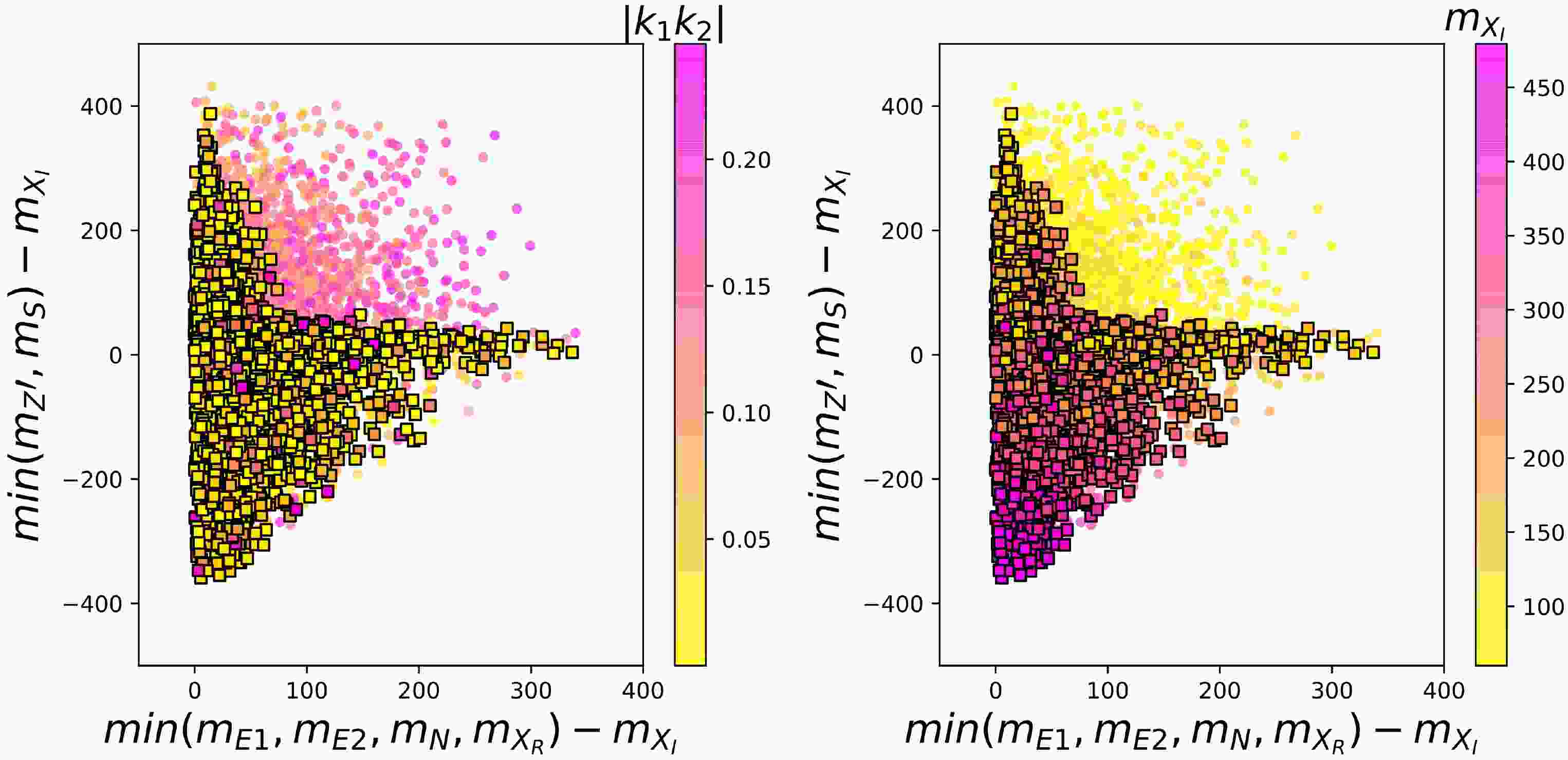
 g-2 anomaly within 2\sigma ranges in Fig. 1. From Fig. 1 , we find that the correct DM relic density can be obtained for most of the parameter region of \min(m_{E_1},\; m_{E_2},\; m_N,\; m_{X_R})-m_{X_I} < 350 GeV and –400 GeV < \min(m_{Z'},m_S) - m_{X_I}< 400 GeV. The DM relic density is mainly produced via the DM pair-annihilation processes X_IX_I \to \; Z'Z',\; SS for the region of \min(m_{Z'},m_S) < m_{X_I}, coannihilation processes for the region of \min(m_{E_1},\; m_{E_2},\; m_N,\; m_{X_R}) close to m_{X_I} , and X_IX_I \to \mu^+\mu^- for the region of both \min(m_{E_1},\; m_{E_2},\; m_N, m_{X_R})>m_{X_I} and \min(m_{Z'},m_S) > m_{X_I} . However, once the explanation of the muon g-2 anomaly is simultaneously required, most of the region of \min (m_{E_1},\; m_{E_2},\; m_N,\; m_{X_R}) > m_{X_I} and \min(m_{Z'},m_S) > m_{X_I} is ruled out. This is because the muon g-2 anomaly favors small interactions between the vector-like leptons and muon mediated by X_I , and thus, the X_IX_I \to \mu^+\mu^- process fails to produce the correct DM relic density.

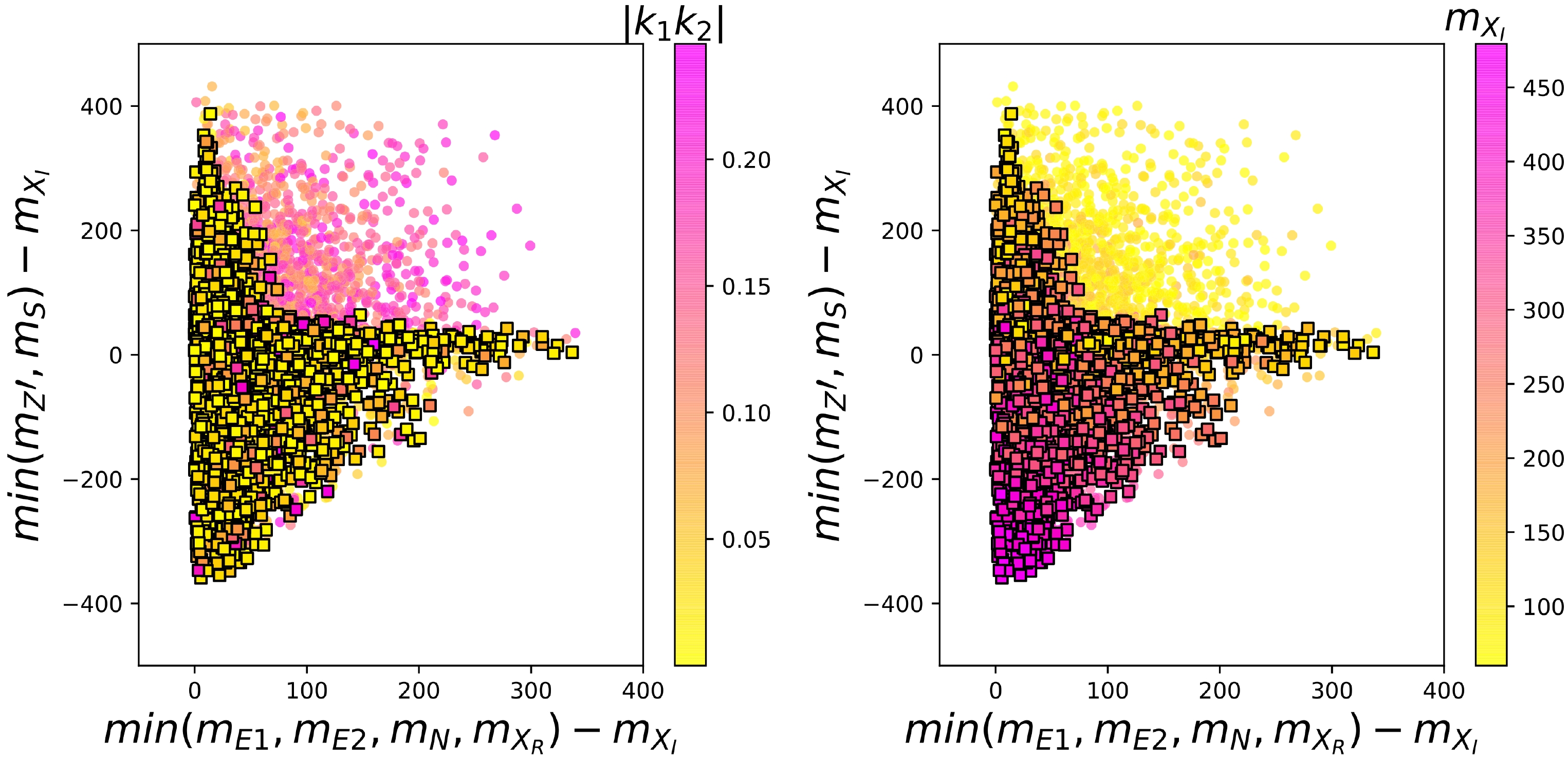
      Figure 1.  (color online) Surviving samples explaining the DM relic density and muon g-2 anomaly while satisfying the constraints from theory, oblique parameter, and 125 GeV Higgs diphoton signal. The circles and squares are excluded and allowed by the DM relic data.

      X_I does not couple to the SM quark, and its couplings to the muon lepton and vector-like leptons are restricted by the muon g-2 anomaly. Therefore, the model can accommodate the bound from the DM direct detection naturally.

    IV.   \boldsymbol{U(1)}_{\boldsymbol{L_\mu-L_\tau}} BREAKING PHASE TRANSITION
    • At high temperatures, the global minimum of the finite-temperature effective potential is at the origin, that is, S U(2)_L\times U(1)_Y\times U(1)_{L_\mu-L_\tau} is unbroken. When the temperature drops, the potential changes and at some point develops a minimum at non-vanishing field values. The PT between the unbroken and the broken phase can proceed in basically two different ways. In a FOPT, at the critical temperature T_C , the two degenerate minima will be at different points in the field space, typically with a potential barrier in between. For a second-order (cross-over) transition, the broken and symmetric minimum are not degenerate until they are at the same point in the field space. In this study, we focus on a first-order U(1)_{L_\mu-L_\tau} breaking PT.

    • A.   Thermal effective potential

    • To examine PT, we first take h_1 , h_2 , and X_r as the field configurations, and obtain the field dependent masses of the scalars (h, S, X_R , X_I ), Goldstone boson ( G,\; \omega,\; G^{\pm} ), gauge boson, and fermions. The field dependent masses of the scalars are as follows:

      {\hat m}^2_{h,S,X_R} ={\rm{eigenvalues}} ( {\widehat{{\mathcal{M}}^2_P}} )\ ,

      (26)

      {\hat m}^2_{G,\omega,X_I} ={\rm{eigenvalues}} ( {\widehat{\mathcal{M}^2_A}}) \ ,

      (27)

      \begin{array}{*{20}{l}} {\hat m}^2_{G^\pm} = \lambda_H h_1^2 - \lambda_H v_h^2 \ , \end{array}

      (28)

      with

      \begin{aligned}[b] \widehat{\mathcal{M}^2_P}_{11} &=3 \lambda_{H} h^2_1 - \lambda_{H} v_h^2\\ \widehat{\mathcal{M}^2_P}_{22} &=- \lambda_S v_S^2 + 3 \lambda_S h_2^2 + { \lambda_{SX} \over 2} X_r^2\\ \widehat{\mathcal{M}^2_P}_{33} &=m_X^2+\sqrt{2}\mu h_2 + { \lambda_{SX} \over 2} h_2^2 + 3 \lambda_X X_r^2\\ \widehat{\mathcal{M}^2_P}_{23} &=\widehat{\mathcal{M}^2_P}_{32}=\sqrt{2} \mu X_r + \lambda_{SX} h_2 X_r \\ \widehat{\mathcal{M}^2_P}_{12} &=\widehat{\mathcal{M}^2_P}_{21}=\widehat{\mathcal{M}^2_P}_{13} =\widehat{\mathcal{M}^2_P}_{31}=0\\ \widehat{\mathcal{M}^2_A}_{11} &= \lambda_{H} h^2_1 - \lambda_{H} v_h^2\\ \widehat{\mathcal{M}^2_A}_{22} &=- \lambda_{S} v_S^2 + \lambda_S h^{2}_{2}+ { \lambda_{SX} \over 2} X_r^{2}\\ \widehat{\mathcal{M}^2_A}_{33} &=m_X^2-\sqrt{2} \mu h_2 + \lambda_X X^{2}_{r}+ { \lambda_{SX} \over 2} h_2^{2}\\ \widehat{\mathcal{M}^2_A}_{23} &=\widehat{\mathcal{M}^2_A}_{32}=-\sqrt{2} \mu X_r\\ \widehat{\mathcal{M}^2_A}_{12} &=\widehat{\mathcal{M}^2_A}_{21}=\widehat{\mathcal{M}^2_A}_{13}=\widehat{\mathcal{M}^2_A}_{31}=0. \end{aligned}

      (29)

      The field dependent masses of the gauge boson are

      {\hat m}^2_{W^\pm} = {1\over 4} g^2 h^{2}_{1}, \quad {\hat m}^2_{Z} = {1\over 4} (g^2+g'^2) h^{2}_{1},

      (30)

      {\hat m}^2_{\gamma}=0 , \quad {\hat m}^2_{Z'} = q_x^2 g_{Z'}^2 (4h^{2}_{2}+X^2_{r}),

      (31)

      The field dependent masses of the vector-like lepton are

      \widehat{\mathcal{M}}^2_{E_1,E_2,\mu} ={\rm{eigenvalues}} ( \widehat{\mathcal{M}_E}\widehat{\mathcal{M}_E}^T )

      (32)

      with

      \begin{array}{*{20}{l}} && \widehat{\mathcal{M}_E}= \begin{pmatrix} m_1 & \quad y_2 h_{1} & \quad \kappa_1 X_r\\ y_1 h_{1} & \quad m_2 & \quad 0\\ 0 & \quad \kappa_2 X_r & \quad \dfrac{m_{\mu} h_1}{v_h} \end{pmatrix} . \end{array}

      (33)

      For the quarks of the SM, we only consider the top quark,

      \widehat{\mathcal{M}^2_{t}} =y_t^2 h_1^2

      (34)

      with y_t=m_t/v_h .

      To examine the U(1)_{L_\mu-L_\tau} breaking PT, we need to study the thermal effective potential V_{\rm eff} in terms of the classical fields ( h_1,h_2,X_r ), which is composed of four parts:

      \begin{aligned}[b] V_{\rm eff} (h_1,h_2,X_r,T)=&V_{0}(h_1,h_2,X_r) + V_{\rm CW}(h_1,h_2,X_r) \\&+ V_{\rm CT}(h_1,h_2,X_r) + V_{T}(h_1,h_2,X_r,T)\\& + V_{\rm ring}(h_1,h_2,X_r,T). \end{aligned}

      (35)

      V_{0} is the tree-level potential, V_{\rm CW} is the Coleman-Weinberg (CW) potential [51], V_{\rm CT} is the counter term, V_{T} is the thermal correction [52], and V_{\rm ring} is the resummed daisy corrections [53, 54]. In this study, we calculate V_{\rm eff} in the Landau gauge.

      The tree-level potential V_0 in terms of the classical fields ( h_1,h_2,X_r ) from Eq. (2) is as follows:

      \begin{aligned}[b] V_0(h_1,h_2,X_r)=& -\frac{\mu_h^2}{2} h_1^2 - \frac{\mu_S^2}{2} h_2^2 + \frac{m_X^2}{2} X_r^2 + \frac{\mu}{\sqrt{2}} h_2 X_r^2\\ &+\frac{\lambda_H}{4} h_1^4 + \frac{\lambda_S}{4} h_2^4 + \frac{\lambda_X}{4} X_r^4 + \frac{\lambda_{SX}}{4} X_r^2 h_2^2 . \end{aligned}

      (36)

      The CW potential in the \overline{\rm MS} scheme at 1-loop level has the form [51]

      \begin{aligned}[b] V_{\rm CW}(h_{1},h_{2},X_r) =& \sum\limits_{i} (-1)^{2s_i} n_i\frac{ {\hat m}_i^4 (h_{1},h_{2},X_r)}{64\pi^2}\\&\times\left[\ln \frac{ {\hat m}_i^2 (h_{1},h_{2},X_r)}{Q^2}-C_i\right] \; \ , \end{aligned}

      (37)

      where i=h,S,X_R,X_I,G,\omega,G^\pm,W^\pm,Z,Z',t,E_1,E_2,\mu , and s_i is the spin of particle i. Q is a renormalization scale, and we take Q=m_S . Constant C_i =\dfrac{3}{2} for scalars or fermions and C_i = \dfrac{5}{6} for gauge bosons. n_i is the number of degree of freedom,

      \begin{aligned}[b] &n_h=n_S=n_{X_R}=n_{X_I}=n_G=n_{\omega}=1\\ &n_{G^\pm}=2,\; \; n_{W^\pm}=6,\; n_{Z}=n_{Z'}=3\\ &n_{t}=12,\; \; n_{E_1}=n_{E_2}=n_{\mu}=4. \end{aligned}

      (38)

      With V_{\rm CW} being included in the potential, the minimization conditions of the scalar potential and CP-even mass matrix will be shifted slightly. To maintain these relations, the counter terms V_{\rm ct} should be added,

      \begin{aligned}[b] V_{\rm CT}=&\delta m_1^2 h_{1}^2+\delta m_2^2 h_{2}^2 + \delta m_X^2 X_r^2 + \delta \lambda_H h_{1}^4+\delta \lambda_{S} h_{2}^4\\ & +\delta \lambda_X X_{r}^4 + \delta \mu X_r^2 h_2 +\delta \lambda_{SX} h_2^2 X_r^2. \end{aligned}

      (39)

      The relevant coefficients are determined by

      \begin{aligned}[b]& \frac{\partial V_{\rm CT}}{\partial h_{1}} = -\frac{\partial V_{\rm CW}}{\partial h_{1}}\;, \quad \frac{\partial V_{\rm CT}}{\partial h_{2}} = -\frac{\partial V_{\rm CW}}{\partial h_{2}},\; \\& \frac{\partial V_{\rm CT}}{\partial X_r} = -\frac{\partial V_{\rm CW}}{\partial X_r}, \end{aligned}

      (40)

      \begin{aligned}[b]& \frac{\partial^{2} V_{\rm CT}}{\partial h_{1}\partial h_{1}} = - \frac{\partial^{2} V_{\rm CW}}{\partial h_{1}\partial h_{1}}\;, \quad \frac{\partial^{2} V_{\rm CT}}{\partial h_{2}\partial h_{2}} = - \frac{\partial^{2} V_{\rm CW}}{\partial h_{2}\partial h_{2}}\;,\\& \frac{\partial^{2} V_{\rm CT}}{\partial X_{r}\partial X_{r}} = - \frac{\partial^{2} V_{\rm CW}}{\partial X_{r}\partial X_{r}}\;,\quad \frac{\partial^{2} V_{\rm CT}}{\partial h_{1}\partial h_{2}} = - \frac{\partial^{2} V_{\rm CW}}{\partial h_{1}\partial h_{2}}\;,\\& \frac{\partial^{2} V_{\rm CT}}{\partial h_1\partial X_r} = - \frac{\partial^{2} V_{\rm CW}}{\partial h_1\partial X_r}\;, \quad \frac{\partial^{2} V_{\rm CT}}{\partial h_2\partial X_r} = - \frac{\partial^{2} V_{\rm CW}}{\partial h_2\partial X_r}\;, \quad \end{aligned}

      (41)

      which are evaluated at the EW minimum of \{ h_{1}=v_h, h_{2}=v_S, X_r=0 \} on both sides. As a result, the VeVs of h_{1} , h_{2} , X_r and the CP-even mass matrix will not be shifted. We verify that the following relations hold true

      \frac{\partial^{2} V_{\rm CW}}{\partial h_{1}\partial h_{2}} =0\;, \quad \frac{\partial^{2} V_{\rm CW}}{\partial h_{1}\partial X_{r}} =0\;.

      (42)

      For the left seven equations, eight parameters need to be fixed, and thus, one renormalization constant is left for determination. We choose to use \delta m_1^2 , \delta m_2^2 , \delta m_X^2 , \delta \lambda_H , \delta \lambda_{S} , \delta \lambda_X , \delta \lambda_{SX} , and set \delta \mu=0 . It is a well-known problem that the second derivative of the CW potential in the vacuum suffers from logarithmic divergences originating from the vanishing Goldstone masses. To avoid the problems with infrared divergent Goldstone contributions, we simply remove the Goldstone corrections in the renormalization conditions following the approaches of [55, 56]. This is simply a change of renormalization conditions, and the shift it causes in the potential shape is negligible.

      The thermal contributions V_T to the potential can be written as [52]

      V_{\rm th}(h_{1},h_{2},X_r,T) = \frac{T^4}{2\pi^2}\, \sum\limits_i n_i J_{B,F}\left( \frac{ {\hat m}_i^2(h_{1},h_{2},X_r)}{T^2}\right)\;,

      (43)

      where i=h,S,X_R,X_I,G,\omega,G^\pm,W^\pm,Z,Z',t,E_1,E_2,\mu , and the functions J_{B,F} are

      J_{B,F}(y) = \pm \int_0^\infty\, {\rm d} x\, x^2\, \ln\left[1\mp {\rm exp}\left(-\sqrt{x^2+y}\right)\right].

      (44)

      Finally, the thermal corrections with resumed ring diagrams are given [53, 54].

      \begin{aligned}[b] V_{\rm ring}\left(h_{1},h_{2},X_r, T\right) =&-\frac{T}{12\pi }\sum\limits_{i} n_{i}\Big[ \left( \bar{M}_{i}^{2}\left(h_{1},h_{2},X_r,T\right) \right)^{\frac{3}{2}}\\&-\left( {\hat m}_{i}^{2}\left(h_{1},h_{2},X_r,T\right) \right)^{\frac{3}{2}}\Big] , \end{aligned}

      (45)

      where i=h,S,X_R,X_I,G,\omega,G^\pm,W^\pm_L,Z_L,Z'_L,\gamma_L . W^\pm_L,~ Z_L, Z'_L , and \gamma_L are the longitudinal gauge bosons with n_{W^\pm_L}=2, n_{Z_L}=n_{Z'_L}=n_{\gamma_L}=1. The thermal Debye masses \bar{M}_{i}^{2}\left(h_{1},h_2, X_r, T\right) for the CP-even and CP-odd scalar fields are the eigenvalues of the full mass matrix,

      \begin{array}{*{20}{l}} \bar{M}_{i}^{2}\left( h_{1},h_{2},X_r,T\right) ={\rm eigenvalues} \left[\widehat{\mathcal{M}_{X}^2}\left( h_{1},h_{2},X_r\right) +\Pi _{X}(T)\right] , \end{array}

      (46)

      where \Pi_X ( X=P,A ) are given by

      \begin{aligned}[b] (\Pi_{P,A})_{11} =& \left[{9g^2\over 2} + {3g'^2\over 2} + 12y_t^2 + 4(y_2^2+y_1^2) +12 \lambda_{H} \right] {T^2 \over 24} \\ (\Pi_{P,A})_{22} =& \left[8 \lambda_S + 2 \lambda_{SX} + 24q_x^2 g^2_{Z'} \right] {T^2 \over 24} \\ (\Pi_{P,A})_{33} =& \left[8 \lambda_X + 2 \lambda_{SX} + 6q_x^2 g^2_{Z'} + 2\kappa_1^2+4\kappa_2^2 \right] {T^2 \over 24} \\ (\Pi_{P,A})_{12} =&(\Pi_{P,A})_{21} =(\Pi_{P,A})_{13} =(\Pi_{P,A})_{31} \\ =&(\Pi_{P,A})_{32} =(\Pi_{P,A})_{23} =0. \end{aligned}

      (47)

      The thermal Debye mass of G^{\pm} is

      \begin{array}{*{20}{l}} \bar{M}_{G^+G^-}^{2}\left( h_{1},h_{2},X_r,T\right) = \lambda_H h_1^2 - \lambda_H v_h^2 +\Pi _{P11}. \end{array}

      (48)

      The Debye masses of longitudinal gauge bosons are

      \begin{aligned}[b] \bar{M}_{W^{\pm}_L}^2 \left( h_{1},h_{2},X_r,T\right)=& {1 \over 4} g^2 h^2_1 + {11\over 6} g^2 T^2, \\ \bar{M}_{Z_L,\gamma_L}^{2}\left( h_{1},h_{2},X_r,T\right) =&\frac{1}{8}\left(g^2+g'^2\right)\left(h_1^2+\frac{22}{3}T^2\right) \pm \frac{1}{2}\Delta, \end{aligned}

      \begin{aligned}[b] \bar{M}_{Z'_L}^2\left( h_{1},h_{2},X_r,T\right) =& q_x^2 g_{Z'}^2 (4h^{2}_{2}+X^2_{r})\\& + {1\over 6} g^2_{Z'} T^2 \left[12-12q_x+ 16q_x^2\right], \end{aligned}

      (49)

      with \Delta=\sqrt{\left[\dfrac{1}{4}\left(g^2-g'^2\right)\left(h_1^2+\dfrac{22}{3}T^2\right)\right]^2+\dfrac{1}{4}g^2 g'^2 h_1^2} .

      In Fig. 2, we display the scatter plots achieving FOFP and accommodating the DM relic density, muon g-2 anomaly, and various constraints mentioned previously. We observe that the strength of FOPT is sensitive to the parameter \lambda_S . As \lambda_S decreases, the the critical temperature T_C tends to decrease, and the strength of FOPT tends to increase. We choose two benchmark points (BPs) to show how the PT happens. The input parameters of BP1 and BP2 are listed in Table 2, and their phase histories are presented in Fig. 3 on the field configurations versus temperature plane. For BP1 and BP2, the potential minima at any temperatures always locate at \langle X_r\rangle =0. As the universe cools, a FOPT takes place during which h_2 acquires a nonzero VeV and the other two fields remain zero. As the temperature continues to decrease, h_1 starts to develop a nonzero VeV during the second PT, which is of second-order. Finally, the observed vacuum is obtained at the present temperature.

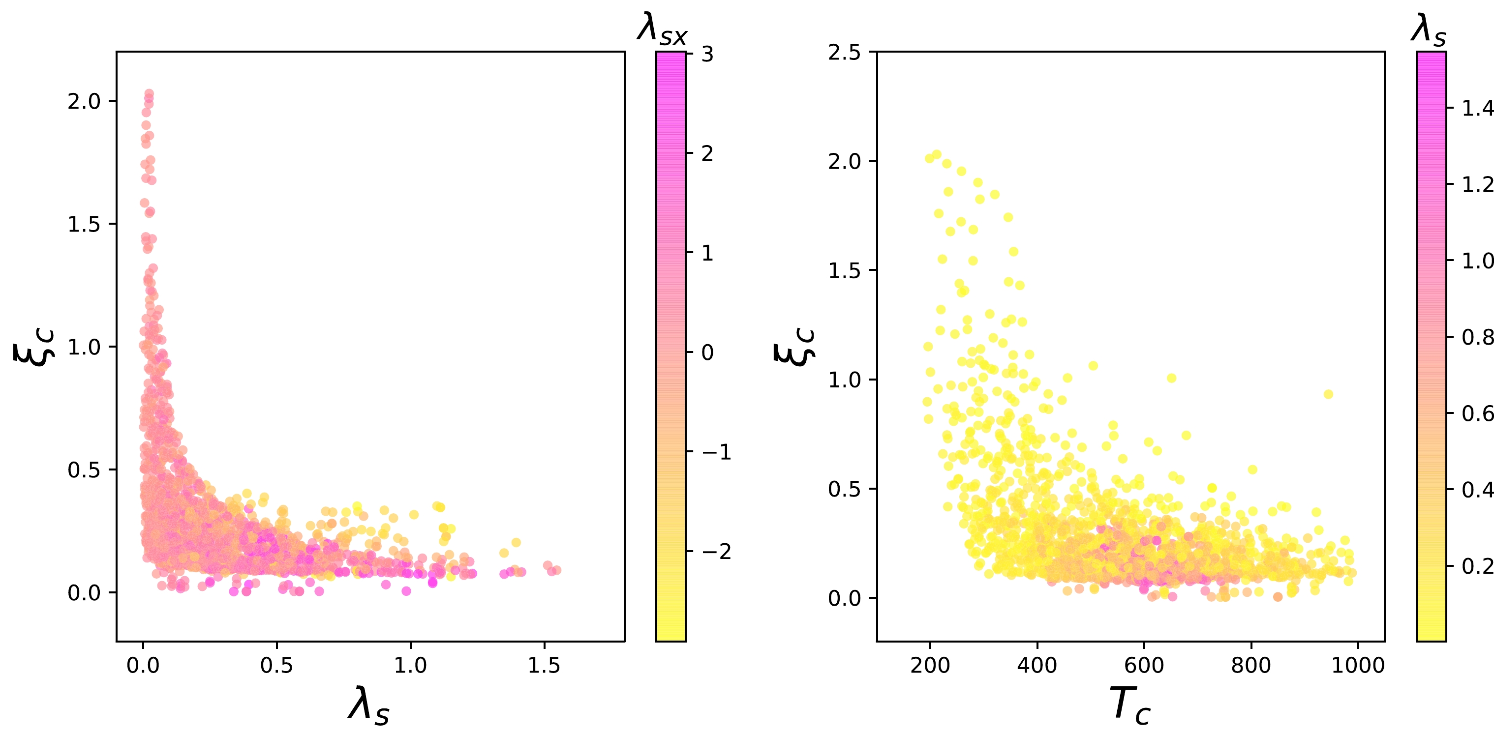
      Figure 2.  (color online) Surviving samples achieving FOFP and accommodating the DM relic density, muon g-2 anomaly, and various constraints mentioned previously. \xi_C=\dfrac{<h_2>}{T_C} denotes the strength of the U(1)_{L_\mu-L_\tau} breaking FOPT at the critical temperature T_C .

      \lambda_{SX}\lambda_{X}\lambda_{s}k_{1}k_{2}s_Ls_Rg_Z\primem_{X_I}/GeV
      {BP1}0.2981.4780.0670.00610.1130.2540.481302.9
      {BP2}0.3040.3370.017−0.0164−0.280−0.3740.319319.2
      m_{X_R}/GeVm_{E_1}/GeVm_{E_2}/GeVm_Z\prime/GeVm_S/GeV
      {BP1}410.2357.4454.6308.4117.1
      {BP2}331.4363.8469.0312.391.6

      Table 2.  Input parameters for BP1 and BP2.

      Figure 3.  (color online) Phase histories of BP1 and BP2. The field configuration X_r is not shown since the minima at any temperature locate at \langle X_r\rangle = 0.

    V.   COLLIDER AND GRAVITATIONAL WAVE SIGNATURE

      A.   Limits from the collider experiments

    • As the U(1)_{L_\mu-L_\tau} gauge boson Z' does not couple to quarks, Z' is rather difficult to produce at the LHC. Vector-like leptons are mainly a pair produced at the LHC via the electroweak processes mediated by the SM gauge bosons, and E_{1,2} \to \mu X_I and N\to \nu_\mu X_I are the main decay modes of vector-like leptons. Thus, we employ the ATLAS analysis of 2\ell+E_T^{\rm miss} with 139 fb ^{-1} integrated luminosity data to restrict our model [57], which is implemented in the \textsf{MadAnalysis5} [5860] assuming a 95% confidence level for the exclusion limit. The simulations for the samples are performed using {\mathrm{MG5}}\_{\mathrm{aMC-3.3.2}} [61] with \mathrm{PYTHIA8} [62] and \mathrm{Delphes-3.2.0} [63].

      In Fig. 4, we employ the ATLAS analysis of 2\ell+E_T^{\rm miss} at the LHC to restrict the parameter space, which has been satisfied by the DM relic density, muon g-2 , FOPT, and various constraints discussed above. Fig. 4 indicates that the DM mass is allowed to be as low as 100 GeV when the value of \min(m_{E_1},\; m_{E_2})-m_{X_I} is small. This is because the muon from the vector-like lepton decay has soft energy, and its detection efficiency is decreased at the LHC. As the DM mass increases, the value of \min(m_{E_1},\; m_{E_2})-m_{X_I} increases, and the lightest charged vector-like lepton is allowed to have a larger mass.

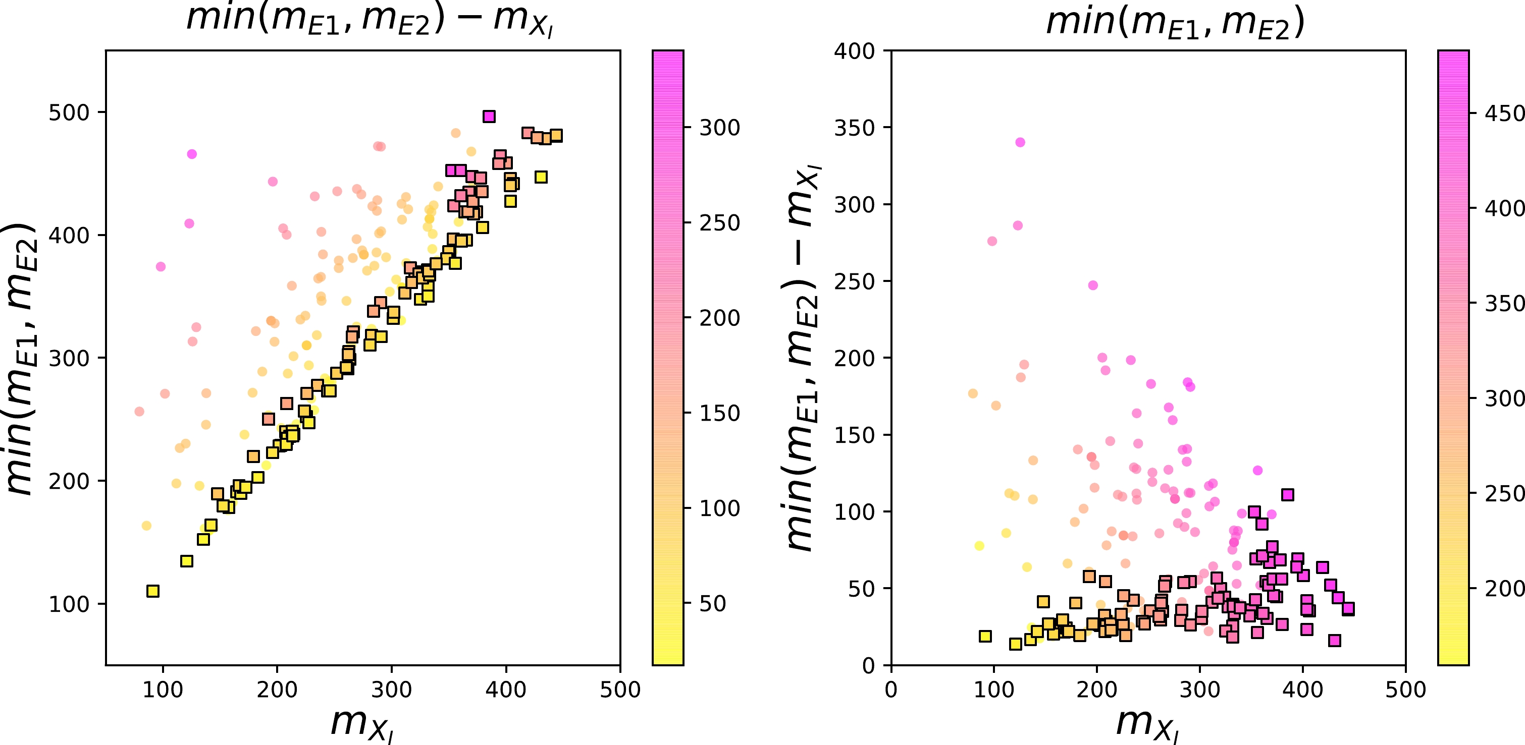
      Figure 4.  (color online) All the samples achieve FOFP and accommodate the DM relic density, muon g-2 anomaly, and various constraints mentioned previously. The circles and squares are excluded and allowed by the direct searches for 2\ell+E^{\rm miss}_T at the LHC.

    • B.   Gravitational wave signature

    • Stochastic GWs are produced during a FOPT via bubble collision, sound waves in the plasma, and magneto-hydrodynamics turbulence. As most of the PT energy is pumped into the surrounding fluid shells, making sound waves the dominant contribution to GWs, we will focus on the GW spectrum from the sound waves in the plasma.

      The sound wave spectra can be expressed as functions of two FOPT parameters β and α,

      \frac{\beta}{H_n}=T\frac{{\rm d} (S_3(T)/T)}{{\rm d} T}\Big|_{T=T_n}\; ,\; \; \; \; \alpha=\frac{\Delta\rho}{\rho_R}=\frac{\Delta\rho}{\pi^2 g_{\ast} T_n^4/30}\;.

      (50)

      Here, H_n is the Hubble parameter at the nucleation temperature T_n , and g_{\ast} is the effective number of relativistic degrees of freedom. β characterizes the approximate inverse time duration of the strong first-order PT, and α is defined as the vacuum energy released from the PT normalized by the total radiation energy density \rho_R at T_n .

      The GW spectrum from the sound waves can be expressed by [64]

      \begin{aligned}[b] \Omega_{ \rm{sw}}h^{2} = & 2.65\times10^{-6}\left( \frac{H_{n}}{\beta}\right)\left(\frac{\kappa_{v} \alpha}{1+\alpha} \right)^{2} \left( \frac{100}{g_{\ast}}\right)^{1/3} v_w \\ &\times \left(\frac{f}{f_{sw}} \right)^{3} \left( \frac{7}{4+3(f/f_{ \rm{sw}})^{2}} \right) ^{7/2} \Upsilon(\tau_{sw})\ , \end{aligned}

      (51)

      where v_w is the wall velocity, and we take v_w=c_s=\sqrt{1/3} , with c_s being the sound velocity. f_{sw} is the present peak frequency of the spectrum,

      f_{sw} \ = \ 1.9\times10^{-5}\frac{1}{v_w}\left(\frac{\beta}{H_{n}} \right) \left( \frac{T_{n}}{100 \rm{GeV}} \right) \left( \frac{g_{\ast}}{100}\right)^{1/6} \rm{Hz} \,.

      (52)

      \kappa_{v} is the fraction of latent heat transformed into the kinetic energy of the fluid [65],

      \kappa_v \simeq \frac{\alpha^{2/5}} {0.017 + (0.997 + \alpha)^{2/5}}.

      (53)

      The suppression factor of Eq. (51) [66],

      \Upsilon(\tau_{sw})=1-\frac{1}{\sqrt{1+2\tau_{sw}H_n}},

      (54)

      appears due to the finite lifetime \tau_{sw} of the sound waves [67, 68],

      \tau_{sw}=\frac{\tilde{v}_W(8\pi)^{1/3}}{\beta \bar{U}_f}, \; \;\; \bar{U}^2_f=\frac{3}{4}\frac{\kappa_v\alpha}{1+\alpha}.

      (55)

      We calculate GW spectra for thousands of parameter points accommodating the muon g-2 , DM relic density, and exclusion limits of the LHC direct searches, and find that all the peak strengths are below the sensitivity curve of BBO. Approximately 10% of the survived points can generate U-DECIGO sensitive gravitational wave, including BP1 and BP2. These points favor a small \lambda_S for which the strength of FOPT tends to have a large value. The GW spectra of BP1 and BP2 are shown along with expected sensitivities of various future interferometer experiments in Fig. 5. The lowest peak frequency is 0.003 HZ from BP1, and the highest peak frequency is 0.2 HZ from BP2.

      Figure 5.  (color online) Gravitational wave spectra for BP1 and BP2.

    VI.   CONCLUSION
    • We study an extra U(1)_{L_\mu-L_\tau} gauge symmetry extension of the standard model by considering the dark matter, muon g-2 anomaly, U(1)_{L_\mu-L_\tau} breaking PT, GW spectra, and bound from the direct detection at the LHC. The following conclusions were drawn. (i) A joint explanation of the dark matter relic density and muon g-2 anomaly rules out the region where both \min(m_{E_1}, m_{E_2},m_N,m_{X_R}) and \min(m_{Z'},m_S) are much larger than m_{X_I} . (ii) A first-order U(1)_{L_\mu-L_\tau} breaking PT can be achieved in the parameter space explaining the DM relic density and muon g-2 anomaly simultaneously, and the corresponding gravitational wave spectra can reach the sensitivity of U-DECIGO. (iii) The mass spectra of the vector-like leptons and dark matter are stringently restricted by the direct searches at the LHC.

Reference (68)

目录

/

DownLoad:  Full-Size Img  PowerPoint
Return
Return