-
The energy production in stars [1] and the associated nucleosynthesis [2–4] as well as supernova explosion dynamics [5] are still not fully understood. Nuclei heavier than iron are mostly formed by neutron capture processes, either the slow neutron capture process (s-process) or rapid neutron capture process (r-process) [2, 3]. Here, the terms slow and rapid consider whether neutron capture proceeds at rates lower or higher than those of typical beta decays occurring along the respective nucleosynthesis path. Slow neutron capture (in particular, that including isotopes across and beyond the neutron magic number N = 50 up to N = 126) is attributed to the final evolutionary stages of red giants (called asymptotic giant branch (AGB) stars). The s-process takes place when
$ 0.3 < T_9<1 $ and the neutron density$ N_n $ $ \approx $ $ 10^8 $ cm$ ^{-3} $ [6].In this paper, we focus on the competition between the
$ ^{95-98} $ Mo(n,γ)$ ^{96-99} $ Mo and$ ^{95-98} $ Mo$ \,\rightarrow $ $ ^{95-98} $ Tc + e +$ \nu_e $ processes within the framework of the statistical code TALYS v1.96 and the proton neutron quasi particle random phase approximation (pn-QRPA) model. The Maxwellian averaged cross-section (MACS) of$ ^{95-98} $ Mo is a crucial quantity in determining the radiative neutron capture rates. Many researchers have theoretically and experimentally studied the neutron capture cross-sections of Mo isotopes at different energy ranges [7–10]. Saumi et al. [7] studied the MACS for the nuclei participating in the s-process and p-process nucleosynthesis around N = 50. They constructed a microscopic optical-model potential by the folding DDM3Y nucleon-nucleon interaction with the radial matter density of the target obtained from the relativistic mean-field (RMF) approximation. Their computed MACSs at$ kT $ = 30 keV for$ ^{95-98} $ Mo(n,γ)$ ^{96-99} $ Mo were 212, 113, 299, and 73.8 mb, respectively. The neutron capture cross-sections of seven stable isotopes of Mo have been measured using a 40 m station of the Oak Ridge Electron Linear Accelerator (ORELA) in the energy range (3$ < $ $ E_{n} $ $ < $ 90) keV [11]. Recently [12], the capture cross-section and transmission of natural Mo were studied using an accurate neutron-nucleus reaction measurement instrument (ANNRI) situated in the Material Life and Science Facility (MLF) at J-PARC. Experimental analyses of capture cross-sections for$ ^{94,\,95,\,96} $ Mo isotopes have been conducted at the neutron time-of-flight facilities n_TOF at CERN and GELINA at JRC-Geel using samples with an enrichment exceeding 95% for each isotope [13]. The transmission parameters obtained in the experiment have been used to validate the resonance parameter files for Mo isotopes. Massimi et al. [14] measured the neutron capture cross-section in EAR1 and EAR2 at the n_TOF facility to reduce the uncertainty in the presently known data for the stable$ ^{94,\,95,\,96} $ Mo isotopes.$ ^{98} $ Mo is the stable and most abundant isotope, with an abundance of 24.13%. Understanding the thermal neutron cross-section and resonance integral for the$ ^{98} $ Mo(n,γ)$ ^{99} $ Mo reaction is crucial owing to the utilization of neutron activation cross-section data in the production of$ ^{99} $ Mo and its potential applications in various studies related to neutron-matter interactions [15]. The existing literature contains numerous experimental and evaluated datasets on the thermal neutron capture cross-section and resonance integrals for the$ ^{98} $ Mo(n,γ)$ ^{99} $ Mo reaction. The authors in Ref. [16] studied the cross-section of$ ^{98} $ Mo(n,γ)$ ^{99} $ Mo using a monochromatic thermal neutron beam at low energy. Their obtained cross-sections were 116$ \pm $ 7 and 91$ \pm $ 5 mb at energies of 0.0334 and 0.0536 eV, respectively.The nuclei (
$ ^{95-98} $ Mo) suggested in the present work are stable isotopes of Mo at the terrestrial environment. The temperature conditions that exist in the stellar matter are so intense (10$ ^9 $ K) that the excited states of parent nuclei have considerable occupation probability. Thus, the individual excited states make measurable contributions to the total stellar weak rates [17]. Therefore, the method based on microscopic calculation of rates must include the contributions of all the partial decay rates due to individual parent excited states. This state by state evaluation of weak-interaction mediated rates is the foundation of the pn-QRPA model [18]. The first attempts to calculate the microscopic weak interaction rates for a large number of available nuclei far away from the stability line were performed using the pn-QRPA approach. The pn-QRPA approach can be formulated based on the mean-field basis employing varying forms of potential. Noticeable mentions would include the deformed Nilsson model [19–21], the finite-range droplet model with a folded Yukawa single-particle potential [22, 23], and the Woods–Saxon potential [24, 25].The present study is structured as follows: Sec. II provides a quick overview of the basic formalism for the statistical code (TALYS v1.96) and the pn-QRPA model. Sec. III summarizes the results of our calculations and how they compare to previous findings and measurements. Our findings are summarized in Sec. IV.
-
The TALYS v1.96 code [26] is based on the Hauser-Feshbach theory [27, 28]. The main inputs in the Hauser-Feshbach theory are the nuclear level densities (NLDs), optical model potentials (OMPs), and gamma strength functions (GSFs). The effect of altering the OMPs can be disregarded in favor of the other two components when low-energy neutrons are used as incident particles [29]. The optical model employed in this study is the local OMP [30].
The TALYS v1.96 code used for the simulation of nuclear reactions includes several state of the art nuclear models to cover almost all key reaction mechanisms encountered for light particle-induced nuclear reactions. It provides an extensive range of reaction channels. The possible incident particles can be simulated in the
$ E_i =$ (0.001−200) MeV, and the target nuclides can be from A = 12 onwards. The output of the nuclear reaction includes total cross-sections, angular distributions, energy spectra, double-differential spectra, MACSs, and capture rates. Radiative capture is important in the context of nuclear astrophysics in which a projectile fuses with the target nucleus and emits γ-ray [31–35]. The MACS is used when the energies of the projectiles follow a Maxwellian distribution, such as that in a stellar enviroment. The MACS is an average of the cross-section over a range of energies, weighted by the Maxwell-Boltzmann distribution.$ {\langle \sigma \rangle (kT) = \frac{2}{\sqrt{\pi}(kT)^2}\int_0^\infty E \sigma (E) {\rm exp}\left(\frac{-E}{kT}\right) {\rm d}E,} $

(1) where k is the Boltzmann constant, T is the temperature,
$ \sigma(E) $ is the capture cross-section, and E is the projectile energy. In statistical models for predicting nuclear reactions, level densities are needed at excitation energies where experimental information is not available, and they have to be taken from theoretical model predictions. Together with the OMP, a correct level density is perhaps the most crucial ingredient for a reliable theoretical analysis of cross-sections, angular distributions, and other nuclear quantities. NLDs are crucial structure ingredients in statistical computations. In the cases where experimental information is not available, they have to be taken from theoretical model predictions. In the present analysis, we employed the back-shifted Fermi gas model (BSFM) as the NLD. The BSFM was used for the entire energy range by treating the pairing energy as an adjustable parameter$ \begin{align} {\rho_{F}^{\rm tot}(E_x) = \frac{1}{\sqrt{2\pi}\sigma}\frac{\sqrt{\pi}}{12}\frac{{\rm exp}(2\sqrt{aU})}{a^{1/4}U^{5/4}}}, \end{align} $

(2) where σ is the spin cut-off parameter, which represents the width of the angular momentum distribution, U is the effective excitation energy, and a is the level density parameter defined below:
$ \begin{aligned} {a = \tilde{a}\left(1+\delta W \frac{1-{\rm exp}(-\gamma U)}{U}\right)},\\ \rm where\; \; \tilde{a}=\alpha A+\beta A^{2/3}, \end{aligned}$

(3) where
$ \tilde{a} $ is the asymptotic level density without any shell effects, A is the mass number, and α, β, and γ are global parameters that need to be determined to give the best average level density description over a whole range of nuclides.$ \delta W $ gives the shell correction energy, and the damping parameter γ determines how rapidly a approaches to$ \tilde{a} $ . For the best fitting, one can readjust the a to achieve the desired value of cross-section and nuclear reaction rates. For further investigations, one can refer to [36]. Different GSFs are included in TALYS v1.96; among them, the Brink-Axel model is used for all transitions except for$ E1 $ [26]. The GSF$ f_{XL} $ for the Brink-Axel gives the distribution of the average reduced partial transition width as a function of the photon energy$ E_{\gamma} $ $ \begin{align} {{f_{XL}(E_{\gamma}) = K_{XL}\frac{\sigma_{XL}E_{\gamma}\Gamma^2_{XL}}{(E_{\gamma}^2-E_{XL}^2)^2+(E_{\gamma}\Gamma^2_{XL})^2}},} \end{align} $

(4) where
$ E_{XL} $ is the energy,$ \Gamma_{XL} $ is the width, and$ \sigma_{XL} $ is the giant resonance strength. For$ E1 $ transitions, TALYS v1.96 utilizes the Kopecky-Uhl model by default$ \begin{aligned}[b] f_{XL}(E_{\gamma}, T)=\;&K_{XL}\Bigg[\frac{E_{\gamma}\tilde{\Gamma}_{E1}(E_{\gamma},\,T)}{(E_{\gamma}^2-E_{E1}^2)^2+E^2_{\gamma}\tilde{\Gamma}_{E1,\,T}(E_{\gamma})^2} \\&+ \frac{0.7\Gamma_{E1}4\pi^2T^2}{E_{E1}^3}\Bigg]\sigma_{E1}\Gamma_{E1}, \end{aligned} $

(5) and
$ {\tilde{\Gamma}_{E1}(E_{\gamma},\,T) = \Gamma_{E1}\frac{E_{\gamma}^2+4\pi^2{\dfrac{E_n+S_n-\Delta-E_{\gamma}}{a(S_n)}}}{E_{E1}^2},} $

(6) where
$ \tilde{\Gamma}(E_{\gamma}) $ represents the energy-dependent damping width,$ E_n $ is the incident energy of neutrons,$ S_n $ is the neutron seperation energy, and Δ is the correction for pairing. As mentioned earlier, a represents the level density parameter at$ S_n $ . The Gogny-HFB+QRPA dipole strength function is employed for the large-scale calculations of the$ E1 $ and$ M1 $ absorption γ-ray strength function within the framework of the axially symmetric deformed quasiparticle random phase approximation (QRPA) based on the finite range D1M Gogny force to the de-excitation strength function [37]. The final$ E1 $ and$ M1 $ strengths, including low-energy contributions (D1M+ QRPA+0lim), can be stated as follows:$ \begin{align} {f_{E1}(\varepsilon_\gamma) = f_{E1}^{\rm QRPA}(\varepsilon_\gamma) + f_{0}U/[1+{\rm e}^{(\varepsilon_\gamma-\varepsilon_0)}]} \end{align} $

(7) $ \begin{align} {f_{M1}(\varepsilon_\gamma) = f_{M1}^{\rm QRPA}(\varepsilon_\gamma) + C\,{\rm e}^{-\eta \varepsilon_\gamma},} \end{align} $

(8) where
$f_{X1}^{\rm QRPA}$ is the D1M+QRPA dipole strength at the photon energy$ \varepsilon_\gamma $ , and U is the excitation energy of the initial de-exciting state.$ f_0 $ ,$ \varepsilon_0 $ , C, and η are freely adjustable parameters. -
The stellar beta decay rates are investigated within the framework of the pn-QRPA. The Hamiltonian for the model is expressed as
$ \begin{align} H^{\rm QRPA} = H^{sp} + V^{\rm pair} + V ^{ph}_{\rm GT} + V^{pp}_{\rm GT}. \end{align} $

(9) The deformed Nilsson potential (
$ H^{sp} $ ) basis is utilized to compute the wave functions and single particle energies. Pairing forces are represented by the second term of Eq. (9) within the framework of the Bardeen–Cooper–Schrieffer (BCS) approximation. Q-values and residual interactions have a considerable influence on the computed electron emission ($ \beta^{-} $ ) rates and associated half-lives [38].$V ^{ph}_{\rm GT}$ (χ (ph)) and$V^{pp}_{\rm GT}$ (κ (pp)), known as the residual interactions, are taken into account for the calculation of the Gamow Tellar (GT) strength. For a thorough definition of χ and κ, as well as the optimal choice of these parameters, see Refs. [38–40].The
$V^{ph}_{\rm GT}$ interaction is expressed as$ \begin{align} V^{ph}_{\rm GT}= +2\chi\sum^{1}_{\mu= -1}(-1)^{\mu}Y_{\mu}Y^{\dagger}_{-\mu}, \end{align} $

(10) with
$ \begin{align} Y_{\mu}= \sum_{j_{p}m_{p}j_{n}m_{n}}<j_{p}m_{p}\mid t_- \; \sigma_{\mu}\mid j_{n}m_{n}>c^{\dagger}_{j_{p}m_{p}}c_{j_{n}m_{n}}, \end{align} $

(11) whereas the
$ V^{pp}_{\rm GT} $ interaction is defined as$ \begin{align} V^{pp}_{\rm GT}= -2\kappa\sum^{1}_{\mu= -1}(-1)^{\mu}P^{\dagger}_{\mu}P_{-\mu}, \end{align} $

(12) with
$ \begin{aligned} P^{\dagger}_{\mu}=\;& \sum_{j_{p}m_{p}j_{n}m_{n}}<j_{n}m_{n}\mid (t_- \sigma_{\mu})^{\dagger}\mid j_{p}m_{p}>\\ & \times (-1)^{l_{n}+j_{n}-m_{n}}c^{\dagger}_{j_{p}m_{p}}c^{\dagger}_{j_{n}-m_{n}}, \end{aligned} $

(13) where χ and κ are taken from Ref. [40]. Reduced GT transition probabilities are achieved by expressing the QRPA ground state into one-phonon states in the daughter nucleus. Additional input variables for the calculation of weak transitions include the pairing gap (
$ \Delta_{p} $ ,$ \Delta_{n} $ ), nuclear deformation ($ \beta_{2} $ ), threshold-values of energy, and Nilsson potential variables (NPV). We adjusted our computation with nuclear deformation parameters from the most recent analysis [41]. The NPV is taken from [42], and the oscillation constant (which is similar for protons and neutrons) is determined using the equation$ \hbar\omega= 41A^{-{1}/{3}} $ (in MeV). We employed the Nilsson potential for the analysis of the wave functions.$ \beta_{2} $ is used as an input parameter in the Nilsson potential. Primarily, wave functions and single particle energies are calculated on the deformed Nilsson basis. The transformation from the spherical nucleon basis (c$ _{jm}^{+} $ , c$ _{jm} $ ) to the axial symmetric deformed basis (d$ _{m\alpha}^{+} $ , d$ _{m\alpha} $ ) is performed as follows:$ \begin{align} d_{m\alpha}^+=\sum_{j}D_{j}^{m\alpha}c_{jm}^+, \end{align} $

(14) where D
$ _{j}^{m\alpha} $ is a group of Nilsson eigenfunctions with α as an additional quantum number to characterize the Nilsson eigen-states. The BCS formalism is used in the Nilsson basis for the neutron/proton system separately. The diagonalization of the Nilsson Hamiltonian yields the transformation matrices (a detailed explanation can be found in [39, 43]). The globally systematic pairing gap values,$ \Delta_{n} $ =$ \Delta_{p} $ =12$ /\sqrt{A} $ (MeV), are employed in our computation. The Q-values are obtained from the most current assessment of atomic mass data [44]. Further details of Eq. (9) may be obtained from [45]. The computation of terrestrial beta decay half-lives and further information on the formalism utilized to estimate GT transitions in stellar scenarios using the pn-QRPA technique can be found in Refs. [46, 47].The electron emission rates/positron capture rates (
$ \lambda^{(\beta^{-}/pc)}_{ij} $ ) from the parent nucleus (ith-state) to the daughter nucleus (jth-state) is given by$ \begin{align} \lambda^{^{(\beta^-/pc)}}_{ij}=\ln 2\frac{f_{ij}(T,\rho,E_f)}{(ft)_{ij}}, \end{align} $

(15) where
$ (ft)_{ij} $ is related to the reduced transition probability ($ B_{ij} $ ) by$ \begin{align} (ft)_{ij}=D/B_{ij}, \end{align} $

(16) D is taken as
$ 6143 $ s [48], and$ B_{ij} $ is defined as$ \begin{align} B_{ij}=B(F)_{ij}+(g_A/g_{V})^2B(GT)_{ij}, \end{align} $

(17) where B(F) and B(GT) are the Fermi and Gamow Teller reduced transition probabilities, respectively.
$ f_{ij} $ is the phase space factor. Further details can be found in Ref. [47]. Due to the high temperature in the stellar core,$ \beta^{-} $ and positron capture (pc) rates receive only a minor contribution from parent excited energy levels. We utilize the Boltzmann distribution function to compute the occupancy probability of the parent$ i $ th-state:$ \begin{align} P_{i} = \frac {{\rm exp}(-E_{i}/kT)}{\sum_{i=1}^{}{\rm exp}(-E_{i}/kT)}. \end{align} $

(18) Furthermore, the total stellar
$ \beta^{-} $ /$\rm pc$ rates are computed using$ \begin{align} \lambda^{^{(\beta^-/pc)}} = \sum_{ij}P_{i} \lambda_{ij}^{^{(\beta^-/pc)}}. \end{align} $

(19) The summation stands for the computation of all parent and daughter energy levels until the required and desired convergence is achieved. In our present calculations, the large model space (up to 7
$ \hbar\omega $ major oscillatory shells) makes it easier to achieve the desired convergence. The ability to calculate the weak rates of any heavy nuclear species is one of the main advantages of the pn-QRPA technique. -
The total neutron capture rate (
$ \lambda_{(n,\gamma)} $ in the units of$ s^{-1} $ ) is defined as [49]$ \begin{align} \lambda_{(n,\gamma)} = (v_{i}\times \sigma_{i} \times n_n)\,{s^{-1},} \end{align} $

(20) where
$ v_{i} $ is the averaged neutron velocity,$ \sigma_{i} $ is the MACS, and$ n_n $ is the average neutron density for$ T_{9} $ $ < $ 1.$ \begin{align} n_n = \frac{4.3\times10^{36}\rho X_4{\rm e}^{[-(0.197/T_9)^{4.82}]}(\frac{1}{T_9})^{2/3} {\rm e}^{\frac{-47}{(T_9)^{1/3}}}}{\sigma_{22}[1+{\sigma_{i}N_i}/\Sigma\sigma_{22}N_{22}](\frac{T_9}{0.348})^{1/2}} \; \rm {cm^{-3},} \end{align} $

(21) where
$ X_4 $ is the helium mass fraction, ρ is the nuclear matter density, and$T_9 $ is the temperature at the base of the convective shell.$ \sigma_{22} $ is the$ ^{22} $ Ne(n,γ)$ ^{23} $ Ne capture cross-section.$ N_i $ is the abundance of species i, and$ \sigma_{i} $ is the MACS.$ N_{22} $ is the abundance by mass of$ ^{22} $ Ne. We have chosen ρ = 10$ ^{4} $ g cm$ ^{-3} $ ,$ X_4 $ = 0.2, and$ \sigma_{22} $ = 0.4 mb for the calculations of average neutron density. The composition of heavy nuclei at the base of the convective shell is dominated by$ ^{22} $ Ne produced by α- captures on$ ^{14} $ N from the CNO cycle. -
For some applications, such as astrophysical investigations involving nuclei along neutron or proton drip lines, it is crucial to extrapolate the data much beyond the experimentally known region. The NLD and GSFs can now be tested on the experimental data relative to the radiative neutron-capture cross-sections of the
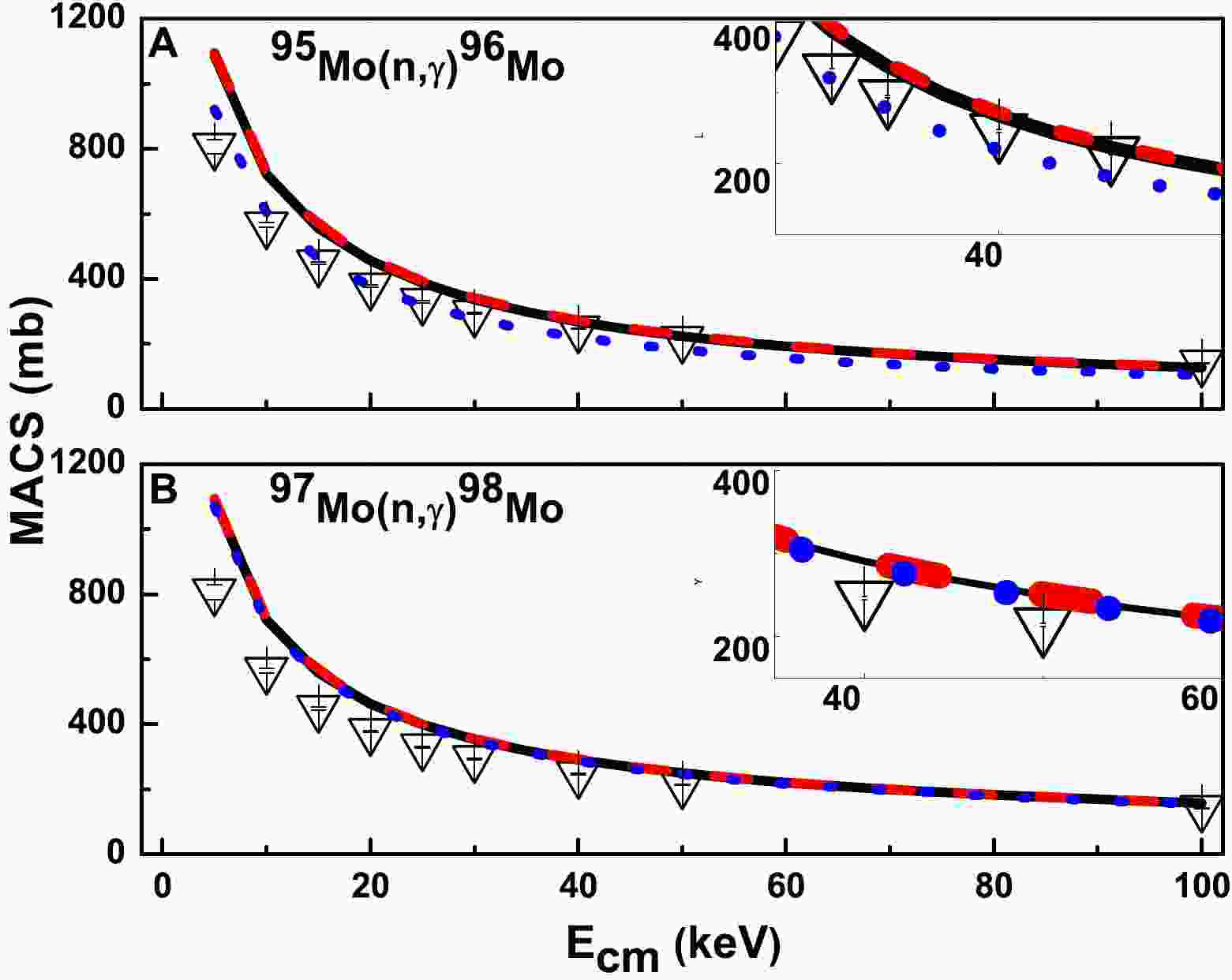
$ ^{95-98} $ Mo(n,γ)$ ^{96-99} $ Mo process. These cross-sections essentially depend on the photon transmission coefficient of the final compound nucleus. Because experiments cannot be conducted at all energies, it is evident that theoretical extrapolations are important for the radiative capture processes. In the present analysis, we employed the NLD model (BSFM) and GSFs (Brink-Axel, Gogny, and Kopecky-Uhl) for the computation of the MACSs of$ ^{95-98} $ Mo. The present-listed Mo isotopes are beta stable in terrestrial environments. Moreover, they have almost stable neutron number configurations, which result in their small (n,γ) cross-sections. For the calculation of MACSs for$ ^{95-98} $ Mo(n,γ)$ ^{96-99} $ Mo, we fixed the BSFM for the NLD and Brink-Axel, Gogny, and Kopecky-Uhl for the GSFs. Together with the findings of Ref. [50], the MACSs for$ ^{95,\,97} $ Mo(n,γ)$ ^{96,\,98} $ Mo within (0.01$ < $ $ kT $ $ < $ 100) keV are depicted in Fig. 1(A), (B). The computed results based on the present model agree well with the data in Ref. [50], and both are below or above the s-process energy ($ kT $ = 30 keV). Note that, in order to achieve the best-fitting with the measured data, we adjusted the parameter a as mentioned in Eq. (3). In the present case, the adjustment parameter a is determined to be 0.5 through adjustment to all available experimental data of the MACS. Similarly, the$ ^{96,\,98} $ Mo(n,γ)$ ^{97,\,99} $ Mo radiative capture processes are analyzed using the BSFM for the NLD and Brink-Axel, Gogny, and Kopecky-Uhl for the GSF. The energy dependent MACSs for$ ^{96} $ Mo and$ ^{98} $ Mo isotopes are depicted in Fig. 2(A), (B) along with the results of Ref. [50]. The computed MACSs at$ kT $ = 30 keV for the analysis of$ ^{96} $ Mo(n,γ)$ ^{97} $ Mo are 121.35 mb (Brink-Axel for the GSF), 124.31 mb (Gogny for the GSF), and 152.29 mb (Kopecky-Uhl for the GSF). It is observed that the present model-based results agree well with the 113 mb MACS at$ kT $ = 30 keV from Ref. [50]. Similarly, the computed MACSs at$ kT $ = 30 keV for the analysis of$ ^{98} $ Mo(n,γ)$ ^{99} $ Mo are 101.28 mb (Brink-Axel for the GSF), 98.42 mb (Gogny for the GSF), and 78.80 mb (Kopecky-Uhl for the GSF). Remarkably, at$ kT $ = 30 keV, the current model-based results agree well with the MACS reported in Ref. [50].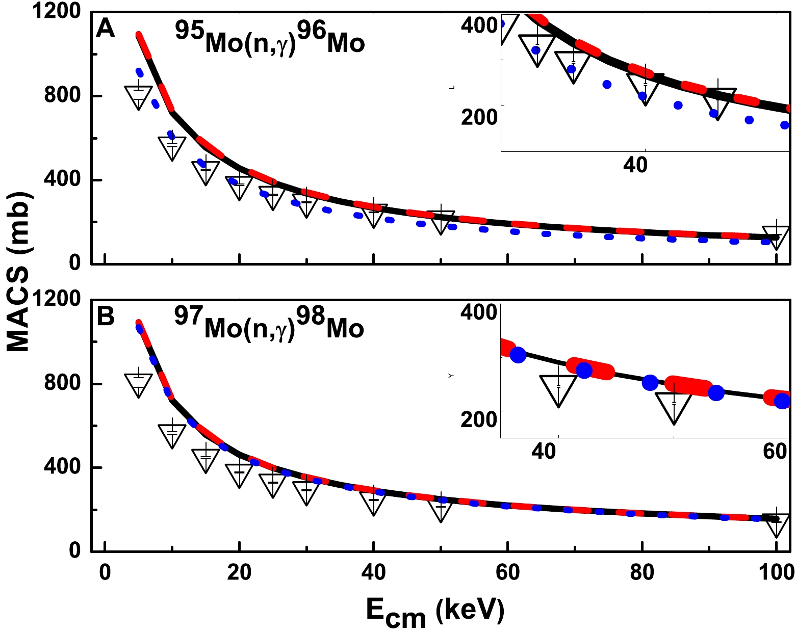
Figure 1. (color online) Total MACS for
$ ^{95,97} $ Mo(n,γ)$ ^{96,\,98} $ Mo along with the measured data ($ \bigtriangledown $ ) [50]. (A) MACS for$ ^{95} $ Mo(n,γ)$ ^{96} $ Mo computed by the BSFM for the NLD with Brink-Axel (solid line), Gogny (dashed line), and Kopecky-Uhl (dotted line) for the GSFs. (B) MACS for$ ^{97} $ Mo(n,γ)$ ^{98} $ Mo computed by the BSFM for the NLD with Brink-Axel (solid line), Gogny (dashed line), and Kopecky-Uhl (dotted line) for the GSFs.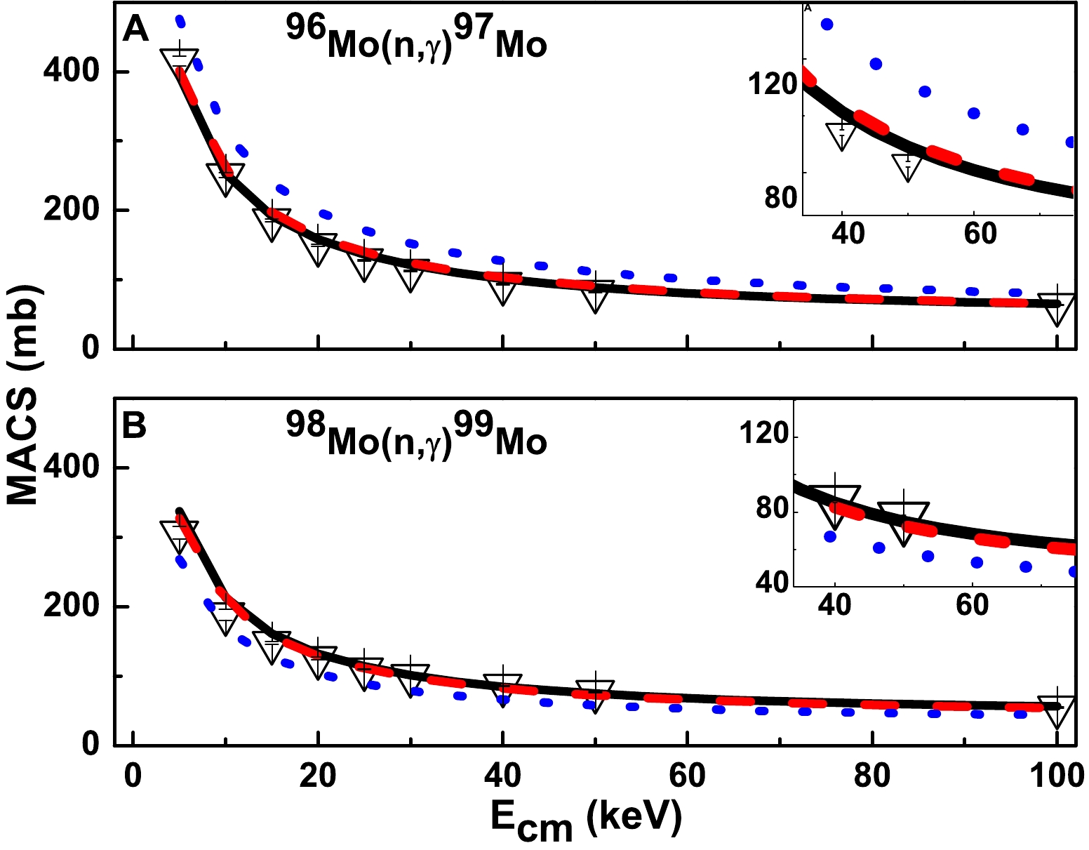
Figure 2. (color online) Total MACS for
$ ^{96,\,98} $ Mo(n,γ)$ ^{97,\,99} $ Mo along with the measured data ($ \bigtriangledown $ ) [50]. (A) MACS for$ ^{96} $ Mo(n,γ)$ ^{97} $ Mo computed by the BSFM for the NLD with Brink-Axel (solid line), Gogny (dashed line), and Kopecky-Uhl (dotted line) for the GSFs. (B) MACS for$ ^{98} $ Mo(n,γ)$ ^{99} $ Mo computed by the BSFM for the NLD with Brink-Axel (solid line), Gogny (dashed line), and Kopecky-Uhl (dotted line) for the GSFs.As mentioned earlier, the nuclei (
$ ^{95-98} $ Mo) in the present work are stable isotopes of Mo at the terrestrial enviroment. However, the temperature conditions that exist in the stellar enviroment are so intense that the excited states of parent nuclei are highly likely to be occupied. Each excited state contributes measurably to the cumulative stellar weak rates. As a result, the approach based on microscopic rate computation must incorporate the contributions of all partial decay rates attributable to the individual parent excited state. For this purpose, we employed the the pn-QRPA framework. The pn-QRPA Hamiltonian defined by Eq. (9) has Nilsson deformed potential and residual interaction terms. In the present study, we employed the nuclear deformation ($ \beta_{2} $ ) from the finite range droplet model (FRDM) [41] as an input parameter for our pn-QRPA model based calculations. The$ \beta_{2} $ values are 0.000 ($ ^{95} $ Mo), 0.150 ($ ^{96} $ Mo), 0.172 ($ ^{97} $ Mo), and 0.206 ($ ^{98} $ Mo). The residual interaction χ and κ values in the present cases are optimized based on Ref. [40] and completely satisfy the model-independent Ikeda sum rules. Based on the optimized values of the residual interactions, we computed the electron emission and positron capture rates. The results of our present investigations are presented in Figs. 3–6 (A)–(C) at densities ρ = (10$ ^{3} $ –10$ ^{5} $ ) g cm$ ^{-3} $ . It is obvious from the results that the electron emission rates are higher than the positron capture rates at lower and higher temperatures. At low density, ρ = 10$ ^{3} $ g cm$ ^{-3} $ , and low temperatures, the$ \lambda_{\beta^{-}} $ values are higher than the$ \lambda_{pc} $ values; however, at high temperatures,$ \lambda_{pc} $ increases gradually because the positron is created at high temperatures. For$ ^{95} $ Mo, there is a clear difference between the$ \lambda_{pc} $ and$ \lambda_{\beta^{-}} $ values at higher densities, as mentioned in Figs. 3–6 (A)–(C). Similarly, Figs. 4–6 (A)–(C) depict the$ \lambda_{pc} $ and$ \lambda_{\beta^{-}} $ values for$ ^{96-98} $ Mo at ρ = (10$ ^{3} $ −10$ ^{5} $ ) g cm$ ^{-3} $ . We noted that the stellar beta decay rates increase with temperature, but for the cases of heavier nuclei of Mo,$ \lambda_{pc} $ and$ \lambda_{\beta^{-}} $ are almost the same at higher temperatures.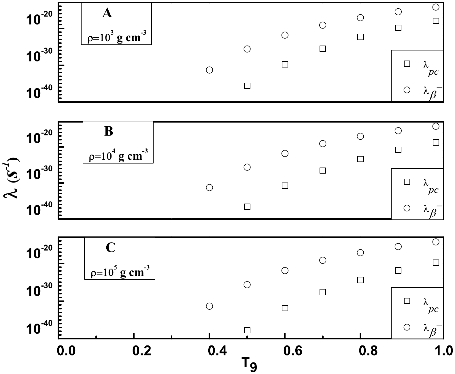
Figure 3.
$ \lambda_{pc} $ and$ \lambda_{\beta^{-}} $ at all densities for the beta decay of$ ^{95} $ Mo.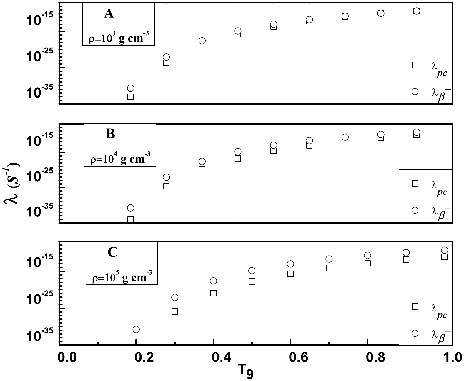
Figure 5.
$ \lambda_{pc} $ and$ \lambda_{\beta^{-}} $ at all densities for the beta decay of$ ^{97} $ Mo.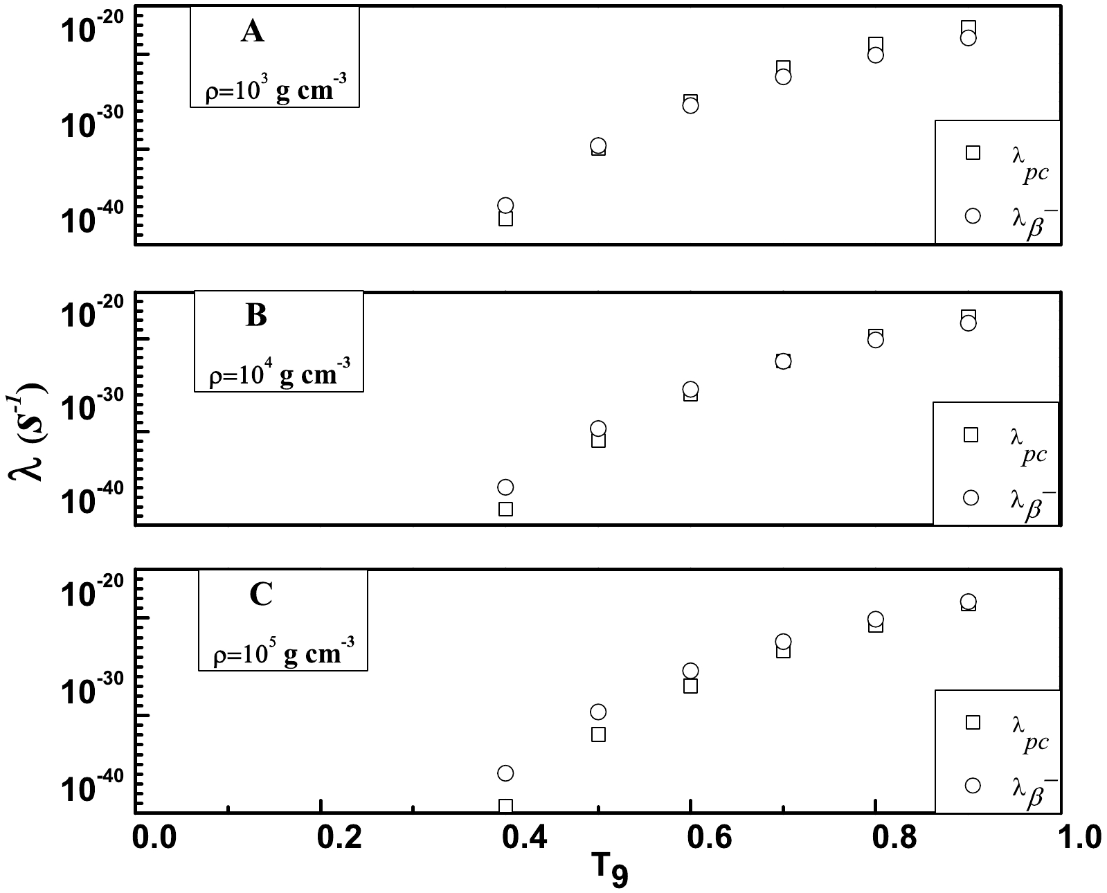
Figure 6.
$ \lambda_{pc} $ and$ \lambda_{\beta} $ at all densities for the beta decay of$ ^{98} $ Mo.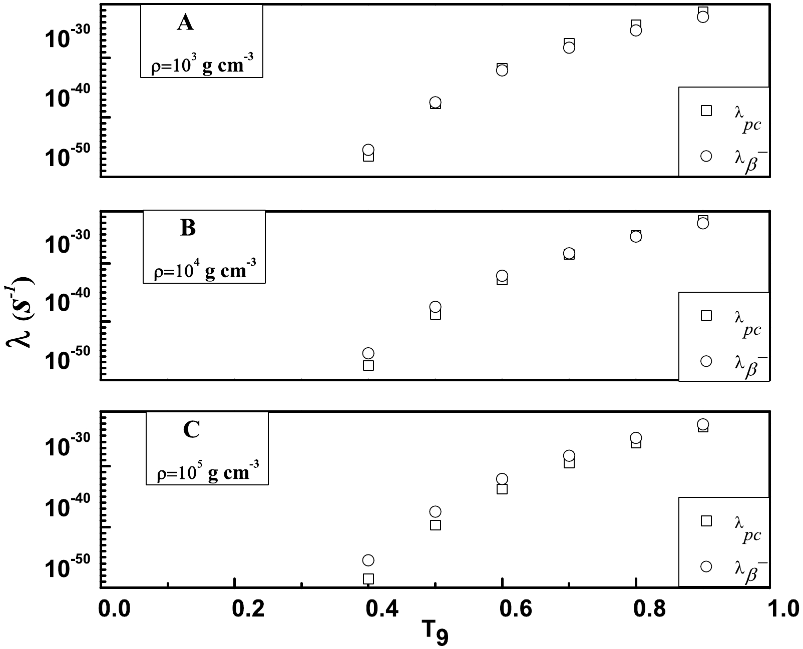
Figure 4.
$ \lambda_{pc} $ and$ \lambda_{\beta^{-}} $ at all densities for the beta decay of$ ^{96} $ Mo.Furthermore, we computed the temperature-dependent neutron capture rates (
$ \lambda_{(n,\,\gamma)} $ ) for$ ^{95-98} $ Mo. For the calculations of$ \lambda_{(n,\,\gamma)} $ , we employed Eq. (20). In the initial set of computations, we identified the best-fitting model combination (in TALYS v1.96) for each isotope; in our investigation, this combination is Brink-Axel as the GSF and BSFM as the NLD. Based on the relevant MACSs, we computed$ \lambda_{(n,\,\gamma)} $ . At$ kT $ = 30 keV, the present computed MACSs for$ ^{95} $ Mo and$ ^{97} $ Mo are 276 and 347 mb, respectively. Employing these cross-sections, the total neutron capture rates for$ ^{95} $ Mo and$ ^{97} $ Mo are$ \lambda_{(n,\,\gamma)} $ = (6.60$ \times $ 10$ ^{-17} $ $ n_n $ ) s$ ^{-1} $ and$ \lambda_{(n,\gamma)} $ = (8.305$ \times $ 10$ ^{-17} $ $ n_n $ ) s$ ^{-1} $ , respectively. Similarly, at$ kT $ = 30 keV, the MACSs for$ ^{96} $ Mo and$ ^{98} $ Mo are 121 and 98 mb, respectively. With these cross-sections, the total capture rates for$ ^{96} $ Mo and$ ^{98} $ Mo are$ \lambda_{(n,\,\gamma)} $ = (2.90$ \times $ 10$ ^{-17} $ $ n_n $ ) s$ ^{-1} $ and$ \lambda_{(n,\,\gamma)} $ = (2.34$ \times $ 10$ ^{-17} $ $ n_n $ ) s$ ^{-1} $ , respectively. At ρ = 10$ ^{4} $ g cm$ ^{-3} $ and$ X_4 $ = 0.2, the present computed$ \lambda_{(n,\,\gamma)} $ and$ \lambda_{(\beta^{-} + pc)} $ values are depicted in Fig. 7 (A)–(D) for the$ ^{95-98} $ Mo + n$ \rightarrow $ $ ^{96-99} $ Mo + γ and$ ^{95-98} $ Mo$ \rightarrow $ $ ^{95-98} $ Tc + e +$ \nu_e $ . Evidently, at lower temperatures, the thermally enhanced beta decay rates are much lower in magnitude than$ \lambda_{(n,\,\gamma)} $ . For example, at$ T_{9} $ = 0.1,$ \lambda_{(n,\,\gamma)} $ = 5.1$ \times $ 10$ ^{-31} $ s$ ^{-1} $ , whereas at the same temperature,$ \lambda_{(\beta^{-} + pc)} $ is 0.97$ \times $ 10$ ^{-100} $ s$ ^{-1} $ for$ ^{95} $ Mo. Similarly, at$ T_{9} $ = 0.5,$ \lambda_{(n,\,\gamma)} $ = 3.5$ \times $ 10$ ^{-02} $ s$ ^{-1} $ and$ \lambda_{(\beta^{-} + pc)} $ is 2.37$ \times $ 10$ ^{-26} $ s$ ^{-1} $ . For$ ^{97} $ Mo, at$ T_{9} $ = 0.1,$ \lambda_{(n,\,\gamma)} $ = 6.4$ \times $ 10$ ^{-31} $ s$ ^{-1} $ , whereas at the same temperature,$ \lambda_{(\beta^{-}+pc)} $ is 5.5$ \times $ 10$ ^{-56} $ s$ ^{-1} $ . However, at$ T_{9} $ = 0.5,$ \lambda_{(n,\,\gamma)} $ = 4.4$ \times $ 10$ ^{-02} $ s$ ^{-1} $ and$ \lambda_{(\beta^{-}+pc)} $ is 1.37$ \times $ 10$ ^{-15} $ s$ ^{-1} $ . In the examined situations of Mo nuclei, the neutron capture rates exceed the thermally enhanced beta decay rates both at lower and higher temperatures.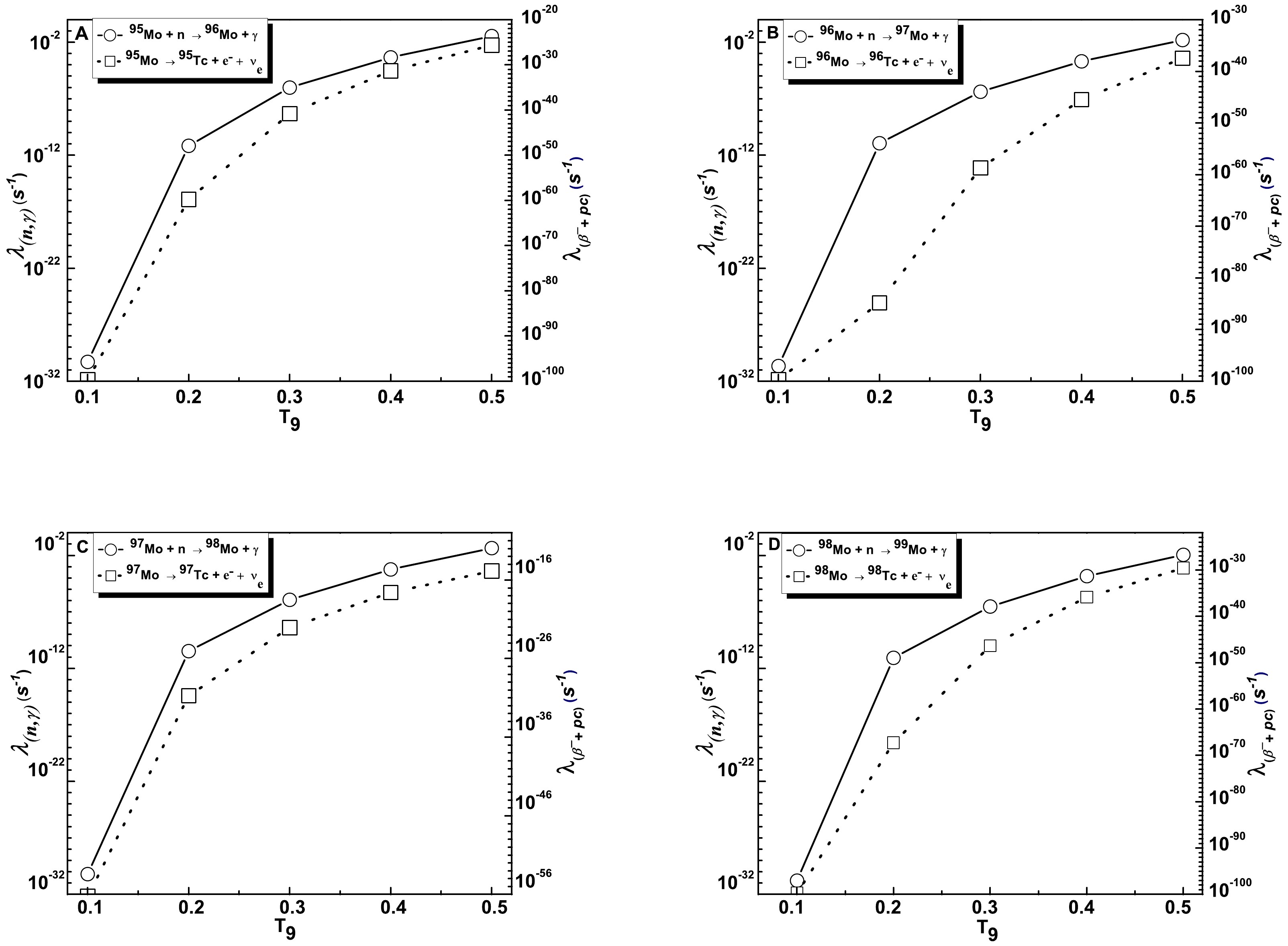
Figure 7. Neutron capture rates (
$ \lambda_{(n,\,\gamma)} $ ) and stellar beta decay rates ($ \lambda_{(\beta^{-}+pc)} $ ) of$ ^{95-98} $ Mo at ρ = 10$ ^{4} $ g cm$ ^{-3} $ ,$ X_4 $ = 0.2, and$ \sigma_{22} $ = 0.4 mb. (A) Computed$ \lambda_{(n,\gamma)} $ and$ \lambda_{(\beta^{-}+pc)} $ for$ ^{95} $ Mo. (B) Computed$ \lambda_{(n,\,\gamma)} $ and$ \lambda_{(\beta^{-}+pc)} $ for$ ^{96} $ Mo. (C) Computed$ \lambda_{(n,\,\gamma)} $ and$ \lambda_{(\beta^{-}+pc)} $ for$ ^{97} $ Mo. (D) Computed$ \lambda_{(n,\,\gamma)} $ and$ \lambda_{(\beta^{-}+pc)} $ for$ ^{98} $ Mo. -
The main findings and inferences are summarized as follows.
1. We examined the MACSs of the (n,γ) process for sets of stable Mo nuclei with magic or nearly magic neutron numbers in the context of the TALYS v1.96 code across a broad energy range. We deduced that the capture cross-section for
$ ^{96,\,98} $ Mo(n,γ)$ ^{97,\,99} $ Mo is lower than that for$ ^{95,\,97} $ Mo(n,γ)$ ^{96,\,98} $ Mo, which is usually included in models of the s-process in AGB stars. Furthermore, we deduced that, among several NLD and GSF models, the BSFM (for the NLD) and Brink-Axel (for the GSF) of TALYS v1.96 are the best fits for the$ ^{95-98} $ Mo(n, γ)$ ^{96-99} $ Mo process. For these nuclei, the Hauser-Feshbach theory prediction accurately reproduces the available experimental data with parameter modifications.2. We computed the
$ \beta^{-} $ /positron capture rates based on the pn-QRPA framework for different densities and temperatures. The pn-QRPA theory effectively calculates the stellar weak interaction rates for$ ^{96-98} $ Mo. Our analysis included a broad model space of 7$ \hbar\omega $ . We computed the stellar weak interaction rates within a wide range of temperatures and densities. We noted that at higher densities, the beta decay rates increase with temperature.3. We compared
$ \lambda_{(n,\,\gamma)} $ and$ \lambda_{(\beta^{-}+pc)} $ under appropriate stellar conditions in the last phase of our investigations. We observed that stellar beta decay rates are lower than neutron capture rates at low and even high temperatures. For example, at$ T_{9} $ = 0.5,$ \lambda_{(n,\gamma)} $ /$ \lambda_{(\beta^{-}+pc)} $ = 1.50$ \times $ 10$ ^{24} $ , 4.27$ \times $ 10$ ^{35} $ , 3.22$ \times $ 10$ ^{13} $ , and 4.48$ \times $ 10$ ^{27} $ for$ ^{95} $ Mo,$ ^{96} $ Mo,$ ^{97} $ Mo, and$ ^{98} $ Mo, respectively. Based on the present investigation, we identified that$ \lambda_{(n,\gamma)} $ is higher than$ \lambda_{\beta} $ .
Re-analysis of temperature dependent neutron capture rates and stellar β-decay rates of 95-98Mo
- Received Date: 2024-02-12
- Available Online: 2024-09-15
Abstract: The neutron capture rates and temperature dependent stellar beta decay rates of Mo isotopes are investigated within the framework of the statistical code TALYS v1.96 and the proton neutron quasi particle random phase approximation (pn-QRPA) model. The Maxwellian average cross-section (MACS) and neutron capture rates for the


 Abstract
 HTML
HTML Reference
 Related
 PDF
PDF




 DownLoad: