


 Abstract
 HTML
HTML Reference
 Related
 PDF
PDF


-
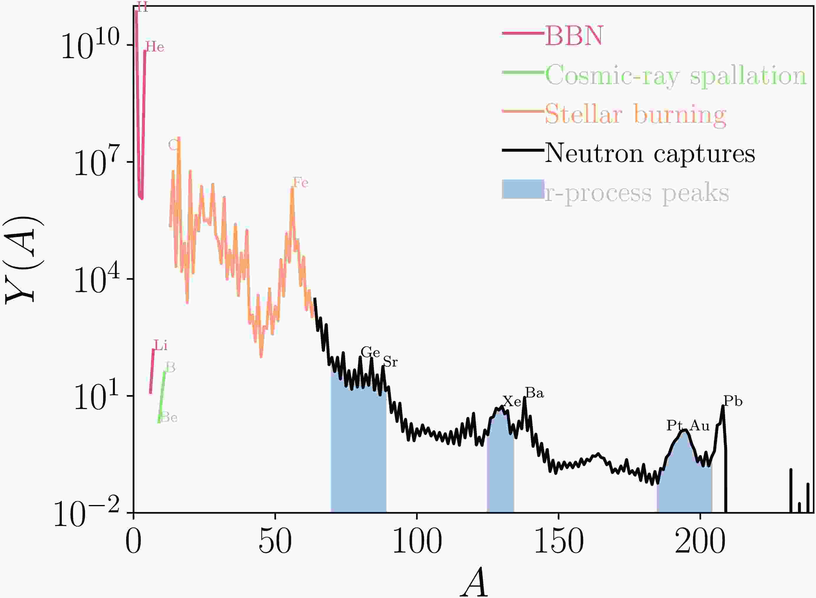
Understanding the details of the nucleosynthesis that leads to the abundance pattern of the elements is a key task of nuclear astrophysics. Experiments with relativistic heavy ion beams (RIB) [1] contribute significantly to understanding the details of the r-process. Analyzing the solar abundance pattern as we know it today provides information for understanding the formation and early history of our solar system [2]. A graph of the abundance pattern is shown in Fig. 1 (data from [3]).

Figure 1. (color online) Element abundance
$ Y_i $ is considered as a function of the mass number$ A_i = N_i + Z_i $ . We have applied the most commonly used scaling, which normalizes the abundance of Silicon to$ Y(\text{Si}) = 10^{6} $ .Hydrogen and helium, the most abundant elements in the universe, were formed by Big Bang Nucleosynthesis (BBN). While some of the lithium may also originate from BBN, there is still a cosmological problem concerning the abundance of 7Li [4]. For the stable isotopes of boron, there are some explanations [5, 6]. All other elements, up to the iron peak, were formed through stellar burning processes. Astrophysical scenarios deal with a large range of parameters in temperature, density, and different environments, and therefore result in different nucleosynthesis processes being predominant. The main processes and concepts were formulated by Burbidge et al. [7] and Cameron [8]. The majority of elements up to the iron peak are generated during the lifecycle of stars. Heavier elements (from gallium to fissile nuclides) are formed by neutron capture reactions.
The abundance of elements in our solar system (Fig. 1) suggests that there are two main processes based on the capture of free neutrons: the slow neutron capture (s-) process, which occurs during the late stage of stellar evolution in asymptotic giant branch (AGB) stars, and the rapid neutron capture (r-) process. It is still an open question what processes exactly provide the environment for the rapid neutron capture process. Most probably, neutron-star mergers and core-collapse supernovae [9] play a role. The s-process and r-process each account for roughly half of the abundance of the heavy elements above the iron peak. In the s-process, a seed nucleus captures a neutron to form an unstable isotope, which undergoes beta decay. The environment allows enough time for the beta decay to take place before the next neutron is captured. In the r-process, the environment is extremely neutron-rich, and therefore multiple neutron captures may occur before beta decay takes place. The neutrino-driven wind of core-collapse supernovae can contribute to the r-process only if the entropy is significantly higher than in most supernova models [10]. The ejecta of compact object mergers, especially when the material of the colliding objects is of very high neutron density, like in neutron stars (NS), can generate an r-process environment with low entropy conditions [11]. In the latter case, the r-process can reach up to the regime of fissionable nuclei (
$ A>250 $ ). This is the case we investigate here. Our study intentionally departs from the mainstream paradigm of r-process nucleosynthesis, which primarily focuses on identifying key nuclei and reactions through sensitivity studies. Instead, we investigate a fundamental mechanistic question: under what conditions can the fission fragment yield distribution (FFYD) directly imprint its signature onto the final r-process abundance pattern? To study key nuclei, we expect further insights from experiments at the HIAF facility (High Intensity Accelerator Facility, Huizhou, Guangdong Province, China) [12, 13] and FAIR (Facility for Antiproton and Ion Research, Darmstadt, Hessen, Germany) [14, 15] in the near future. -
Understanding the details of the nucleosynthesis that leads to the abundance pattern of the elements is a key task of nuclear astrophysics. Experiments with relativistic heavy ion beams (RIB) [1] contribute significantly to understanding the details of the r-process. Analyzing the solar abundance pattern as we know it today provides information for understanding the formation and early history of our solar system [2]. A graph of the abundance pattern is shown in Fig. 1 (data from [3]).
Figure 1. (color online) Element abundance
$ Y_i $ is considered as a function of the mass number$ A_i = N_i + Z_i $ . We have applied the most commonly used scaling, which normalizes the abundance of Silicon to$ Y(\text{Si}) = 10^{6} $ .Hydrogen and helium, the most abundant elements in the universe, were formed by Big Bang Nucleosynthesis (BBN). While some of the lithium may also originate from BBN, there is still a cosmological problem concerning the abundance of 7Li [4]. For the stable isotopes of boron, there are some explanations [5, 6]. All other elements, up to the iron peak, were formed through stellar burning processes. Astrophysical scenarios deal with a large range of parameters in temperature, density, and different environments, and therefore result in different nucleosynthesis processes being predominant. The main processes and concepts were formulated by Burbidge et al. [7] and Cameron [8]. The majority of elements up to the iron peak are generated during the lifecycle of stars. Heavier elements (from gallium to fissile nuclides) are formed by neutron capture reactions.
The abundance of elements in our solar system (Fig. 1) suggests that there are two main processes based on the capture of free neutrons: the slow neutron capture (s-) process, which occurs during the late stage of stellar evolution in asymptotic giant branch (AGB) stars, and the rapid neutron capture (r-) process. It is still an open question what processes exactly provide the environment for the rapid neutron capture process. Most probably, neutron-star mergers and core-collapse supernovae [9] play a role. The s-process and r-process each account for roughly half of the abundance of the heavy elements above the iron peak. In the s-process, a seed nucleus captures a neutron to form an unstable isotope, which undergoes beta decay. The environment allows enough time for the beta decay to take place before the next neutron is captured. In the r-process, the environment is extremely neutron-rich, and therefore multiple neutron captures may occur before beta decay takes place. The neutrino-driven wind of core-collapse supernovae can contribute to the r-process only if the entropy is significantly higher than in most supernova models [10]. The ejecta of compact object mergers, especially when the material of the colliding objects is of very high neutron density, like in neutron stars (NS), can generate an r-process environment with low entropy conditions [11]. In the latter case, the r-process can reach up to the regime of fissionable nuclei (
$ A>250 $ ). This is the case we investigate here. Our study intentionally departs from the mainstream paradigm of r-process nucleosynthesis, which primarily focuses on identifying key nuclei and reactions through sensitivity studies. Instead, we investigate a fundamental mechanistic question: under what conditions can the fission fragment yield distribution (FFYD) directly imprint its signature onto the final r-process abundance pattern? To study key nuclei, we expect further insights from experiments at the HIAF facility (High Intensity Accelerator Facility, Huizhou, Guangdong Province, China) [12, 13] and FAIR (Facility for Antiproton and Ion Research, Darmstadt, Hessen, Germany) [14, 15] in the near future. -
In this work, we use the GEneral description of Fission (GEF) observable model [16]. It is a semi-empirical fission model that is situated between stochastic and empirical models. Here, we introduce the GEF model, with particular emphasis on its application for neutron-rich nuclei. For astrophysical problems, it is necessary to choose a model that can systematically compute the fission properties of many nuclei within a reasonable computing time. In addition to GEF, the FREYA [17] model (which models the properties of fission fragments) and the SPY model [18] (which models the statistical result of yields distribution and the kinetic energy) are also widely used for astrophysical studies. There is also the ABrasion-ABLAtion fission model (shortly, ABLA) [19], which predicts fission fragment yield distributions (FFYD). To the best of our knowledge, this model is no longer updated. The database of experimental data from fission experiments is rather limited; therefore, the models produce different results for the yet unexplored area of nuclei. The GEF model allows the calculation of many fission observables. It outputs: fission yields distribution in Z, N, and A, fragment kinetic energy, angular momentum spectrum, prompt-neutron spectrum, delayed-neutron spectrum, neutron-multiplicity distribution, prompt-gamma ray, delayed-gamma ray spectrum, and gamma-multiplicity distribution. The key innovation of the GEF model lies in using experimental fission data to fit the parameters that form the microscopic correction terms on the potential energy surface (PES). There are many "preferred" charge numbers favored by the fission fragments [20]. The values of the proton number Z and neutron number N of the resulting fission fragments clearly show regularities. These regularities are due to nuclear shell effects in deformed nuclei and are parameterized in GEF. Preferred Z-locations of fragments can be described by:
$ \begin{aligned}[b] &Z_{S1} = 51.5+25\left(\dfrac{Z_{\rm CN}^{1.3}}{A_{\rm CN}}-1.5\right)\\ &Z_{S2} = 54.5+21.67\left(\dfrac{Z_{\rm CN}^{1.3}}{A_{\rm CN}}-1.5\right)\\ &Z_{SA} = 59+21.67\left(\dfrac{Z_{\rm CN}^{1.3}}{A_{\rm CN}}-1.5\right) \end{aligned} $
(1) The standard modes S1, S2, and SA account for asymmetric fission and are related to the fission valleys, located at Z values given in Eq. (1), where CN denotes the compound nucleus. In general, the fission process is a quantum tunneling process. Different fission valleys correspond to different fission barriers. As a result, for most nuclei, the final fission outcome is a superposition of different fission modes. In the GEF model, the contribution
$ K_i $ of each mode i is proportional to the level density$ \rho_i $ of the corresponding fission valley (before the fission barrier) multiplied by the tunneling probability$ P_i $ .$ K_i = \dfrac{\rho_i P_i}{\sum_i\rho_i P_i} $
(2) The number of states per energy interval (level density) is obtained from the constant temperature model (CTM) and is, therefore, characterized by two free parameters: the temperature parameter T and the energy shift parameter
$ E_0 $ [21], with k being the Boltzmann constant.$ \rho_i(E) = \dfrac{1}{kT} {\rm e}^\tfrac{E-E_0}{{k}T} $
(3) It is assumed in GEF that the tunneling probability
$ P_i $ can be characterized by an effective temperature parameter$ T_{\rm eff} $ and the energy difference in the fission valley. With$ E^* $ being the excitation energy and$ E_b $ being the fission barrier in this valley,$ T_{\rm eff} = \dfrac{\hbar\omega}{2\pi} $ , where$ \hbar\omega $ is as in the Hill-Wheeler formula [26].$ P_i = \dfrac{1}{1+{\rm e}^{-\tfrac{E^*-E_b}{kT_{\rm eff}}}} $
(4) For simplicity, in GEF, the fission valleys are considered to be parabolic quantum oscillators along the asymmetry degrees of freedom. Thus, the energy of the system as a function of the Z number is
$ \delta E_i = E_{0i}+C_i(Z_l-Z_i)^2 $
(5) Where the index
$ i $ denotes the different modes,$ Z_l $ is the proton number of the lighter fragment, and$ Z_i $ is the location of the fission mode.$ C_i $ is the stiffness constant for this fission mode. This will result in a Gaussian distribution in the FFYD peaks. The available data of the FFYD show a deformed Gaussian distribution of the S2 mode, which indicates a correction term on the oscillator potential of S2.In order to show the difference in fission yields between GEF2016-1-2 and GEF2019-1-1, we take
$ ^{278}{\rm {Am}} $ as an example. There was an improvement in the GEF code in 2017, which provided more reasonable fission barriers$ E_b $ ; this resulted in a variation of$ P_i $ configurations.Now we compare GEF2016-1-2 and GEF2019-1-1. For GEF2016-1-2,
$ P_i $ is 8.206% of S2 mode (asymmetric), 72.74% of SA mode (asymmetric), and 19.06% of double S1 mode (symmetric); the remaining modes do not contribute. For GEF2019-1-1, the situation is$ P_i $ is 29.75% of S2 mode (asymmetric), 70.24001% of SA mode (asymmetric), with no contribution from the rest.The SA (asymmetric) fission mode produces peaks at
$ A = 105\sim 115 $ and$ A = 160\sim 170 $ , while the S2 (asymmetric) mode generates peaks at$ A = 125 $ and$ 150 $ . The S1 mode corresponds to symmetric fission, yielding a single peak at$ A\sim138 $ . In GEF2016-1-2, symmetric fission (S1) accounts for 19.1% of yields and asymmetric fission (SA + S2) constitutes approximately 81%, resulting in a three-peaked mass distribution. Conversely, GEF2019-1-1 exhibits exclusively asymmetric fission modes (SA and S2), producing a two-peaked yield distribution.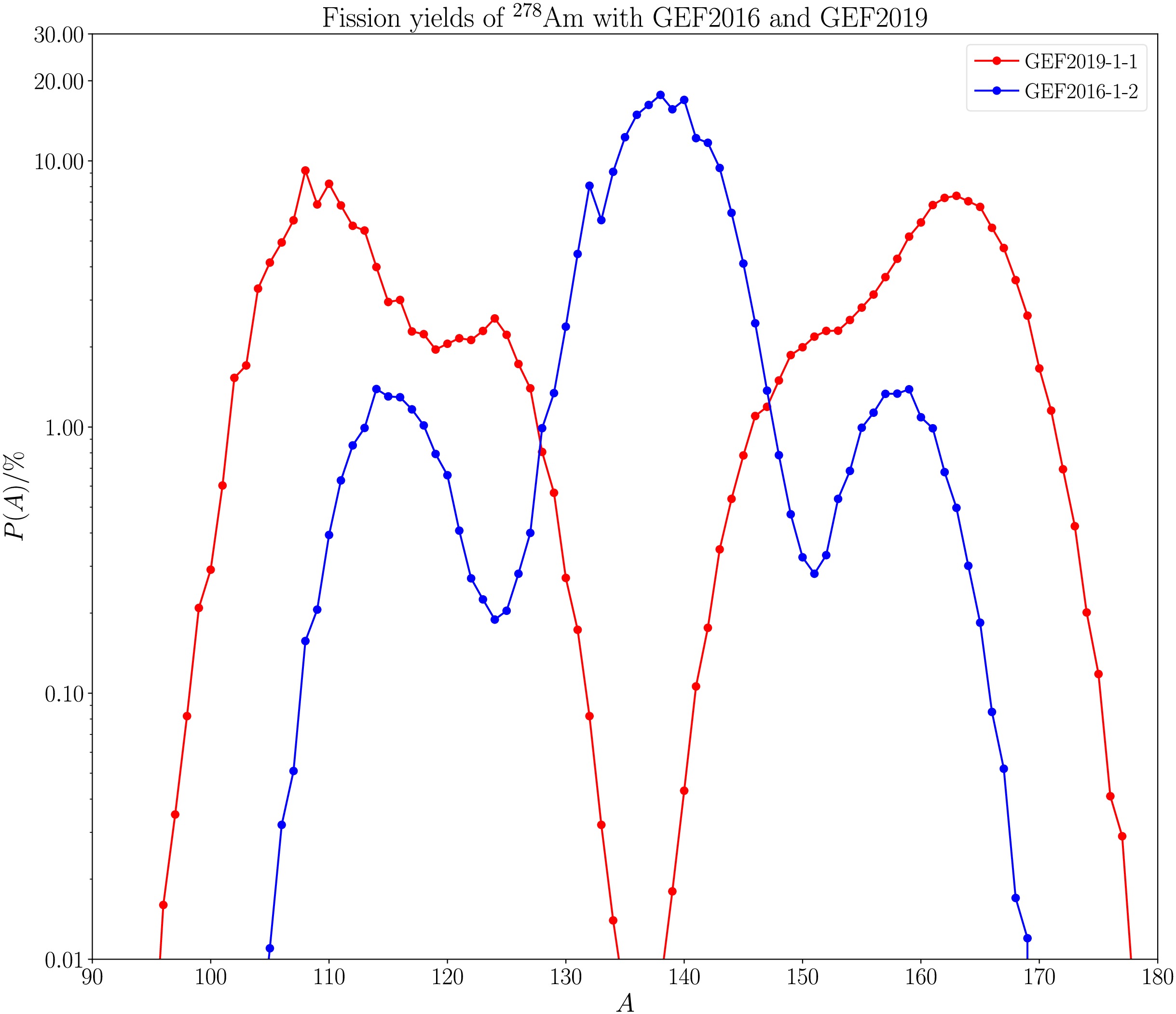
Figure 3. (color online) Fission yields of Am-278 with GEF2016-1-2 and GEF2019-1-1. Fission modes: SA (asymmetric): peaks at
$ A = 105\sim115$ and$ 160\sim170$ ; S2 (asymmetric): peaks at$ A = 125$ and 150; S1 (symmetric): peak at$ A \approx 138$ . GEF2016-1-2 configuration: SA (72.74%), S2 (8.21%), S1 (19.06%) → 3-peak. GEF2019-1-1 configuration: SA (70.24%), S2 (29.75%) → asymmetric 2-peak. -
The environment for the r-process is considered to be the ejecta from neutron-star mergers. Its physical properties are adopted from the simulation [22]. The initial conditions for the r-process calculation are
$ \rho = 10^{10} \; \text{g/cm}^3 $ ,$ s = 5.7 \, k_B $ ,$ Y_e = 0.039 $ , where ρ is the density of the ejecta, s is the entropy per nucleon, and$ Y_e $ stands for the electron fraction. Based on the neutron-induced fission rates provided by [25], we performed the network calculation for different FFYD models using the GSINet code, a well-established tool referenced in prior works ([24, 27] and others). Its numerical methods are detailed in [28]. For this study, we implemented GEF-based fission yields data and validated the implementation through checks for the conservation of mass number and charge, as well as the normalization of fission fragment yields at each timestep. Results are shown in Fig. 2. The black dots represent the solar r-abundance [23], which is the observed solar nuclide abundance reduced by the abundance from the s-process. All other curves are our calculations with different models. The solid lines represent the final abundance pattern from the calculation, and the dashed lines are the fission contribution after the freeze-out. The blue line shows three peaks because the relevant parent nuclei in the GEF-2016-1-2 model favor symmetric fission, whereas the red line shows only 2 peaks, corresponding to the asymmetric fission in GEF-2019-1-1 (red line). The abundance pattern near the 2nd r-process peak is always populated, regardless of whether the FFYD is caused by symmetric or asymmetric fission. This is due to the accumulation of the doubly magic nuclei$ ^{132}_{50}\text{Sn} $ and its isobaric nuclei. However, symmetric FFYD does populate more peak isotopes: the blue and yellow lines at$ A\sim130 $ have higher$ Y(A) $ than the red line in Fig. 2. This shows that symmetric fission produces more peak nuclei than asymmetric fission (see the dashed lines). The height of both "shoulders" of the 2nd r-process peak (the "right shoulder" is located at$ 140 \lt A \lt 170 $ and the "left shoulder" is located at$ 95 \lt A \lt 120 $ ) is determined by the fission fragment distribution; the "right shoulder" corresponds to the heavy fragment, and the "left shoulder" corresponds to the light fragment population.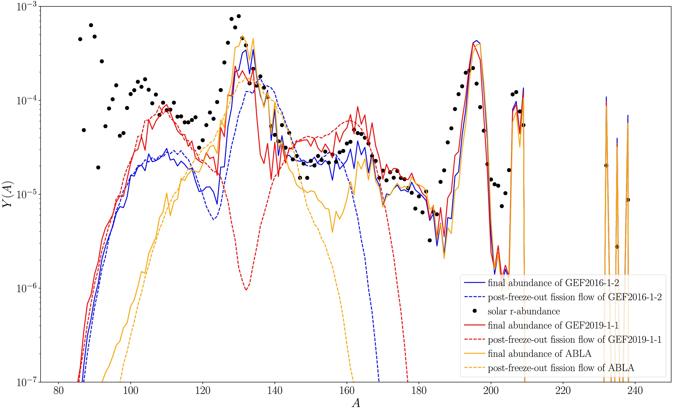
Figure 2. (color online) Calculations based on three models are compared in this figure, as colored in blue (GEF2016-1-2), red (GEF2019-1-1), and orange (ABLA). Each solid line refers to the corresponding final abundances
$ Y(A) $ as a function of mass number A. Each dashed line refers to the corresponding fission flow$ J_{\rm fission} $ that occurs after the r-process freeze-out.Fine details (neighboring mass number nuclei) in the abundance pattern are independent of the FFYD model but depend on other nuclear properties (i.e., neutron separation energy).
For simplicity, we consider fission to be a one-body reaction. Then the fission flow
$ J(Z_p,A_p) $ is defined as the integration of the fission flux$ Y(Z_p,A_p) r(Z_p,A_p) $ over time:$ J(Z_p,A_p) = \int_{t_1}^{t_2} Y(Z_p,A_p) r(Z_p,A_p){\rm d}t, $
(6) where
$ r(Z_p,A_p) $ is the fission rate of the parent nucleus$ (Z_p,A_p) $ . The resulting flow$ J(Z_p,A_p) $ represents the total number of fission events contributed by this parent nucleus throughout the process. Therefore, the parent nuclei with the largest values of J are the dominant contributors to the fission fragment inventory. The fission flow$ J(Z_p,A_p) $ is a diagnostic quantity integrated from the output of the full network calculation. Since the network self-consistently includes the competition between all reaction channels, the abundance$ Y(Z_p,A_p) $ inherently reflects the time-dependent fission branching ratio. Therefore, J represents the total number of fission events that occurred for nucleus$ (Z_p,A_p) $ under the fully competitive conditions of the r-process, making it the appropriate measure to identify the dominant fission parents.Since fission relates to one fission parent and two fission fragments, it will generate the abundance of heavy nuclei. In order to determine the fission flow from the fragment nucleus, one needs to accumulate the fission events that happen in different parent nuclei, since a specific fission fragment can be generated by multiple fission parents.
$ J(Z_d,A_d) = \sum\limits_pJ(Z_p,A_p)*P(Z_d,A_d), $
(7) where
$ P(Z_d,A_d) $ is the yield probability that starting from the fission of a parent nucleus$ (Z_p,A_p) $ , demonstrates the probability of producing a specific fission fragment$ (Z_d,A_d) $ .The fission flow from the parent nuclei is shown in Fig. 4 a) the total flow, b) the fission flow after freeze-out, and c) the fission flow before the freeze-out.
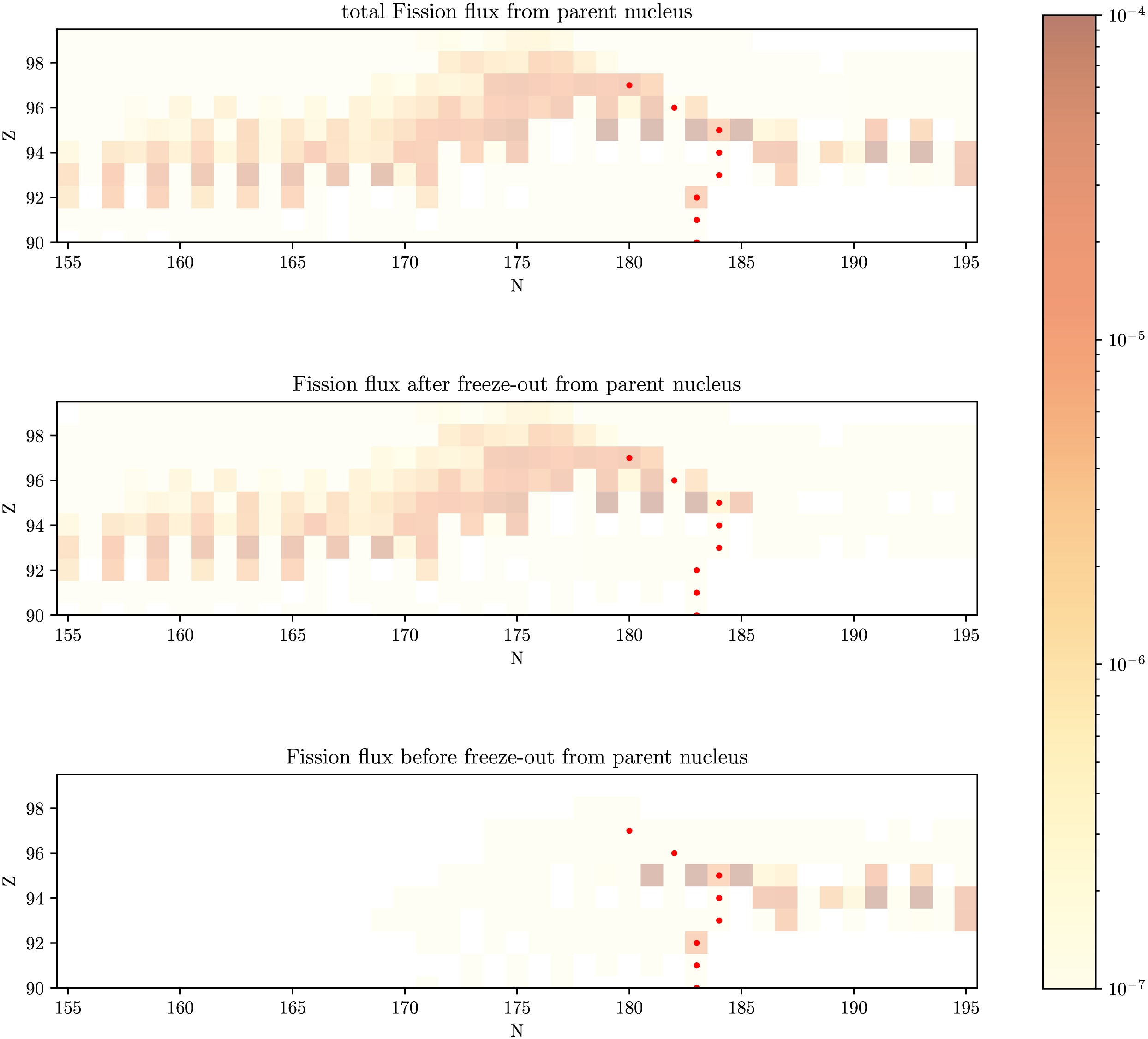
Figure 4. (color online) Fission flow pattern. Color scale: fission flow. Panels from top to bottom: total fission flow pattern; fission flow after the freeze-out; fission flow before freeze-out. Red dots represent the most abundant nuclei in each isotopic chain when the freeze-out occurs. Most of the red dots are also the r-process "waiting points".
Here we used the calculation on GEF-2016-1-2 as an example, while calculations for GEF-2019-1-1 and ABLA give almost identical results because the flow from parent nuclei does not directly depend on the FFYD but on fission rates.
In order to quantify the amount of fission, we apply the concept of fission cycles. Each fission event transforms one nucleus into two daughter nuclei. This change affects the abundance of nuclei. This doubling in number is used to define the fission cycle Λ.
$ \Lambda = {\rm log}_2 \left(\dfrac{Y_{\rm end}}{Y_{\rm start}}\right), $
(8) where
$ Y_{\rm start} $ and$ Y_{\rm end} $ stand for the total abundance of the heavy nuclei at the initial and final times, respectively. Since the increase in the abundance of heavy nuclei is caused by the fission flow$ J_{\rm fission} $ , the relationship between$ Y_{\rm start} $ and$ Y_{\rm end} $ can be written as$ Y_{\rm end} = Y_{\rm start} + J_{\rm fission} $ .Before the freeze-out, the models GEF 2016-1-2, GEF 2019-1-1, and ABLA yield results for the fission cycle
$ \Lambda \approx 1.80 $ , while after freeze-out$ \Lambda \approx 0.33 $ . This means that most of the fission occurs before freeze-out. However, as shown in Fig. 2, the post-freeze-out fission flow$ J_{\rm fission} $ (dashed lines) aligns directly with the final abundance pattern (solid lines), particularly in the shoulder regions ($ 95 \lt A \lt 120 $ and$ 140 \lt A \lt 170 $ ). This demonstrates that while pre-freeze-out fission is quantitatively dominant, it is the fission fragments produced after freeze-out, which are no longer reprocessed by neutron captures, that directly determine the final r-process abundance pattern. -
The environment for the r-process is considered to be the ejecta from neutron-star mergers. Its physical properties are adopted from the simulation [22]. The initial conditions for the r-process calculation are
$ \rho = 10^{10} \; \text{g/cm}^3 $ ,$ s = 5.7 \, k_B $ ,$ Y_e = 0.039 $ , where ρ is the density of the ejecta, s is the entropy per nucleon, and$ Y_e $ stands for the electron fraction. Based on the neutron-induced fission rates provided by [25], we performed the network calculation for different FFYD models using the GSINet code, a well-established tool referenced in prior works ([24, 27] and others). Its numerical methods are detailed in [28]. For this study, we implemented GEF-based fission yields data and validated the implementation through checks for the conservation of mass number and charge, as well as the normalization of fission fragment yields at each timestep. Results are shown in Fig. 2. The black dots represent the solar r-abundance [23], which is the observed solar nuclide abundance reduced by the abundance from the s-process. All other curves are our calculations with different models. The solid lines represent the final abundance pattern from the calculation, and the dashed lines are the fission contribution after the freeze-out. The blue line shows three peaks because the relevant parent nuclei in the GEF-2016-1-2 model favor symmetric fission, whereas the red line shows only 2 peaks, corresponding to the asymmetric fission in GEF-2019-1-1 (red line). The abundance pattern near the 2nd r-process peak is always populated, regardless of whether the FFYD is caused by symmetric or asymmetric fission. This is due to the accumulation of the doubly magic nuclei$ ^{132}_{50}\text{Sn} $ and its isobaric nuclei. However, symmetric FFYD does populate more peak isotopes: the blue and yellow lines at$ A\sim130 $ have higher$ Y(A) $ than the red line in Fig. 2. This shows that symmetric fission produces more peak nuclei than asymmetric fission (see the dashed lines). The height of both "shoulders" of the 2nd r-process peak (the "right shoulder" is located at$ 140 \lt A \lt 170 $ and the "left shoulder" is located at$ 95 \lt A \lt 120 $ ) is determined by the fission fragment distribution; the "right shoulder" corresponds to the heavy fragment, and the "left shoulder" corresponds to the light fragment population.
Figure 2. (color online) Calculations based on three models are compared in this figure, as colored in blue (GEF2016-1-2), red (GEF2019-1-1), and orange (ABLA). Each solid line refers to the corresponding final abundances
$ Y(A) $ as a function of mass number A. Each dashed line refers to the corresponding fission flow$ J_{\rm fission} $ that occurs after the r-process freeze-out.Fine details (neighboring mass number nuclei) in the abundance pattern are independent of the FFYD model but depend on other nuclear properties (i.e., neutron separation energy).
For simplicity, we consider fission to be a one-body reaction. Then the fission flow
$ J(Z_p,A_p) $ is defined as the integration of the fission flux$ Y(Z_p,A_p) r(Z_p,A_p) $ over time:$ J(Z_p,A_p) = \int_{t_1}^{t_2} Y(Z_p,A_p) r(Z_p,A_p){\rm d}t, $
(6) where
$ r(Z_p,A_p) $ is the fission rate of the parent nucleus$ (Z_p,A_p) $ . The resulting flow$ J(Z_p,A_p) $ represents the total number of fission events contributed by this parent nucleus throughout the process. Therefore, the parent nuclei with the largest values of J are the dominant contributors to the fission fragment inventory. The fission flow$ J(Z_p,A_p) $ is a diagnostic quantity integrated from the output of the full network calculation. Since the network self-consistently includes the competition between all reaction channels, the abundance$ Y(Z_p,A_p) $ inherently reflects the time-dependent fission branching ratio. Therefore, J represents the total number of fission events that occurred for nucleus$ (Z_p,A_p) $ under the fully competitive conditions of the r-process, making it the appropriate measure to identify the dominant fission parents.Since fission relates to one fission parent and two fission fragments, it will generate the abundance of heavy nuclei. In order to determine the fission flow from the fragment nucleus, one needs to accumulate the fission events that happen in different parent nuclei, since a specific fission fragment can be generated by multiple fission parents.
$ J(Z_d,A_d) = \sum\limits_pJ(Z_p,A_p)*P(Z_d,A_d), $
(7) where
$ P(Z_d,A_d) $ is the yield probability that starting from the fission of a parent nucleus$ (Z_p,A_p) $ , demonstrates the probability of producing a specific fission fragment$ (Z_d,A_d) $ .The fission flow from the parent nuclei is shown in Fig. 4 a) the total flow, b) the fission flow after freeze-out, and c) the fission flow before the freeze-out.
Figure 4. (color online) Fission flow pattern. Color scale: fission flow. Panels from top to bottom: total fission flow pattern; fission flow after the freeze-out; fission flow before freeze-out. Red dots represent the most abundant nuclei in each isotopic chain when the freeze-out occurs. Most of the red dots are also the r-process "waiting points".
Here we used the calculation on GEF-2016-1-2 as an example, while calculations for GEF-2019-1-1 and ABLA give almost identical results because the flow from parent nuclei does not directly depend on the FFYD but on fission rates.
In order to quantify the amount of fission, we apply the concept of fission cycles. Each fission event transforms one nucleus into two daughter nuclei. This change affects the abundance of nuclei. This doubling in number is used to define the fission cycle Λ.
$ \Lambda = {\rm log}_2 \left(\dfrac{Y_{\rm end}}{Y_{\rm start}}\right), $
(8) where
$ Y_{\rm start} $ and$ Y_{\rm end} $ stand for the total abundance of the heavy nuclei at the initial and final times, respectively. Since the increase in the abundance of heavy nuclei is caused by the fission flow$ J_{\rm fission} $ , the relationship between$ Y_{\rm start} $ and$ Y_{\rm end} $ can be written as$ Y_{\rm end} = Y_{\rm start} + J_{\rm fission} $ .Before the freeze-out, the models GEF 2016-1-2, GEF 2019-1-1, and ABLA yield results for the fission cycle
$ \Lambda \approx 1.80 $ , while after freeze-out$ \Lambda \approx 0.33 $ . This means that most of the fission occurs before freeze-out. However, as shown in Fig. 2, the post-freeze-out fission flow$ J_{\rm fission} $ (dashed lines) aligns directly with the final abundance pattern (solid lines), particularly in the shoulder regions ($ 95 \lt A \lt 120 $ and$ 140 \lt A \lt 170 $ ). This demonstrates that while pre-freeze-out fission is quantitatively dominant, it is the fission fragments produced after freeze-out, which are no longer reprocessed by neutron captures, that directly determine the final r-process abundance pattern. -
In this paper, the role of fission in r-process nucleosynthesis is studied. Several sets of fission fragment yield distributions were applied in the nuclear reaction network calculation. The fission model GEF was studied in detail to discuss the variation range of the r-process abundance pattern arising from differences in the fission yields. We have shown the differences arising from symmetric and asymmetric fission.
We conclude that the second r-process peak (
$ A\sim130 $ ) reflects the effect of double magic numbers. The occurrence of this peak does not depend on the fission yields [24]. However, the height of the peak is influenced by the fission yields, depending on whether it is symmetric or asymmetric. Furthermore, the heights of the left ($ 95< A<120 $ ) and right ($ 140<A<170 $ ) shoulders of the second r-process peak clearly depend on the fission yields. In general, all isotope positions (A, Z) in these two ranges are populated by fission.We also showed the reaction flux of the fission channels that correspond to parent nuclei. We pointed out that most fission happens already before the r-process freeze-out; however, those reactions that occur after the freeze-out determine the final abundance pattern.
-
One of us (B. J.) wishes to thank Prof. Gabriel Martinez-Pinedo for his guidance and support during their stay at GSI Helmholtzzentrum.
-
One of us (B. J.) wishes to thank Prof. Gabriel Martinez-Pinedo for his guidance and support during their stay at GSI Helmholtzzentrum.
-
One of us (B. J.) wishes to thank Prof. Gabriel Martinez-Pinedo for his guidance and support during their stay at GSI Helmholtzzentrum.
Influence of the fission yield distribution on the nucleosynthesis in the r-process induced by neutron-star mergers
- Received Date: 2025-05-27
- Available Online: 2026-05-15
Abstract: We investigate the role of nuclear fission fragment yield distributions in shaping r-process nucleosynthesis within the low-entropy environment of neutron-star-merger ejecta. Our results demonstrate that post-freeze-out fission fragment yields play a critical role in determining the abundance pattern of the second r-process peak and its right shoulder ($ 130 \lt A \lt 170$), even though most fission cycles occur before the r-process freeze-out. This study employs the semi-empirical General Fission (GEF) model to systematically characterize fission properties.


 DownLoad: