


 Abstract
 HTML
HTML Reference
 Related
 PDF
PDF


-
Black holes (BHs) are among the most fascinating objects in the Universe, distinguished by their extraordinarily strong gravitational fields. A defining feature of a BH is the extreme warping of spacetime and bending of light in its vicinity. Theoretically, the image of a BH consists of a central dark region, encircled by luminous emissions from infalling matter and shaped by the gravitational lensing effects of the BH [1]. The study of BH shadows offers crucial insights into fundamental BH properties, including their mass, spin, and the dynamics of surrounding accretion flows [2]. Notably, the boundaries of these shadows, particularly the photon rings, are governed solely by general relativity (GR) and remain independent of specific astrophysical environments. Observations of BH shadows, especially through interferometric methods, provide a powerful tool to probe strong-field gravitational effects governed by relativistic dynamics [3].
In recent years, the Event Horizon Telescope (EHT) has achieved a remarkable milestone by capturing images of the shadows of the supermassive BHs in Messier (M) 87* and Sagittarius (Sgr) A*; the latter is located at the center of our galaxy [4−15]. These images, characterized by a bright emission ring encircling a central dark region, are consistent with the predictions of GR for BH shadows. However, the current observational resolution is insufficient to resolve the intricate photon-ring structures, which remain key targets for future imaging campaigns. Next-generation space-based interferometers have the potential to unveil these fine details, offering a transformative opportunity to test the validity of GR in strong-field regimes and uncover deviations indicative of new physics [16].
Recent years have witnessed significant progress in the study of BH accretion disks and their shadow images, driven by advances in both theoretical modeling and observational techniques. Simplified models of accretion disks have played an important role in BH imaging studies by providing effective approximations to the complex dynamics in the vicinity of BHs. These models leverage gravitational lensing and relativistic effects to simulate plausible BH images. For example, Luminets seminal work introduced a spherically symmetric Schwarzschild BH model, demonstrating how ray-tracing simulations can be used to predict BH shadows and the appearance of accretion disks [17]. This model reveals the pronounced light-bending effects intrinsic to strong gravitational fields. Building on this foundation, Gralla et al. developed an analytical approximation to investigate BH shadow structures, providing a framework that accurately characterizes photon rings and their substructures [18]. This framework provides a powerful tool for interpreting photon-ring features observed by the EHT, capturing key aspects of the strong gravitational field near BHs while avoiding computationally intensive numerical simulations.
Geometrically and optically thin simplified models have also been extensively studied in investigations of BH shadow images. Johnson et al. investigated how different radiation patterns from accretion disks affect BH shadow images, highlighting the influence of disk geometry and dynamics [19]. Using these simplified models, they examined key factors such as disk thickness, flow velocity, and BH spin, laying the groundwork for the development of more sophisticated GR magnetohydrodynamic (GRMHD) models. Vincent et al. employed GR-based numerical simulations to study accretion disks and BH shadows, illustrating how accretion disk properties leave imprints on observed images via processes such as spontaneous emission and plasma dynamics in extreme environments [20]. Integrating a thin-disk simplified model with GRMHD simulations, the authors explored the potential for differentiating between various black holes using observational platforms like the EHT. Beyond these landmark studies, numerous investigations have employed simplified models to explore BH images in diverse gravitational settings, thereby advancing a comprehensive understanding of BH shadow properties across a range of spacetime configurations [21−32, 34−36, 38−40].
Beyond toy-based BH shadow imaging, polarization measurements provide a powerful tool for probing the magnetic fields and plasma dynamics near the event horizon. Polarized light carries essential information about both the geometry and strength of magnetic fields surrounding the BH, as well as the motion of charged particles within the accretion disk. The EHT has successfully captured polarized images of the M87* BH, revealing intricate structures in the magnetic field lines within the emission region [40–41, 43]. These polarization maps are crucial for understanding how magnetohydrodynamic (MHD) processes regulate accretion flows and drive relativistic jet formation. Narayan et al. derived an approximate expression for null geodesics, incorporating the conserved Walker–Penrose constant, to provide analytical estimates of image polarization in a Schwarzschild BH model with a thin accretion disk [44]. Gelles et al. extended this analysis by presenting polarized radiation images using a toy model of equatorial sources around a Kerr BH [45]. Their work highlights how polarization patterns in BH images are shaped by the magnetic field geometry, the BHs intrinsic parameters (such as spin), and the observers inclination angle. Beyond Schwarzschild and Kerr spacetimes, several studies have examined how modified gravity theories might influence BH polarization properties, broadening the scope of theoretical predictions [46−54].
Simulations based on simplified models have proven highly effective in predicting BH shadow and photon-ring structures, as well as in estimating physical parameters such as spin and tilt. These models have also been instrumental in testing alternative theories of gravity by identifying potential deviations from GR [55]. As observational capabilities advance, refining toy models becomes increasingly important for interpreting high-precision data and improving the underlying assumptions of simulations. Current efforts focus on modeling the accretion disk and emission properties surrounding BHs, which are essential for guiding ongoing EHT imaging campaigns [56]. In cases where emission is influenced by spatial and temporal variations, non-uniform, anisotropic, and time-varying Gaussian random fields have proven effective for simulating the emission profiles of accretion disks [57]. This approach captures the stochastic nature of accretion processes, particularly in the innermost regions of the disk where turbulence, magnetic reconnection, and other instabilities create a highly dynamic environment. Such models are essential for accurately representing the complex plasma behavior that shapes observed BH images.
The time variability of BH images presents a compelling avenue of investigation. Time-averaged, high-resolution images from GRMHD simulations reveal that photon rings are persistent and sharply defined features, encapsulating the long-term structure of BH shadows [58]. While fluctuations in the accretion disk can obscure the immediate visibility of the photon ring, these variations tend to average out over time, allowing the underlying relativistic signatures to reemerge. Conversely, the dynamic evolution of the accretion disk induces temporal changes in the shadows appearance, with both the brightness and structure of the photon ring exhibiting short-timescale fluctuations [59]. Accurately predicting these variations poses significant challenges, particularly for upcoming space-based very long baseline interferometry (VLBI) missions. Such missions will observe BH shadows intermittently, often capturing only limited and irregular observational snapshots, complicating efforts to reconstruct the full temporal behavior of these relativistic features.
Current BH imaging models primarily rely on the Kerr BH framework, which describes a BH solely in terms of its mass and spin [4−9]. However, the Kerr model neglects the potential influence of electric or magnetic charges, which could significantly affect photon trajectories and polarization patterns, particularly in scenarios involving interactions with electromagnetic fields in the surrounding plasma. To expand the theoretical landscape of BH imaging, investigating rotating BH models that incorporate magnetic charge, such as the rotating Hayward BH, is crucial. The Hayward BH is a regular BH solution that provides an alternative to the singularities predicted by classical GR [60]. Unlike Kerr BHs, the Hayward model features a regularized core with finite curvature, attributed to quantum gravitational effects. This regularization profoundly impacts the BHs shadow and photon-ring structures. In particular, the interplay of core regularization and spin modifies the shadows size and shape, resulting in distinctive observational signatures potentially detectable with high-precision interferometry [61]. To investigate these effects, we analyzed the optical appearance of Hayward BHs using simplified models for both spherical and thin-disk accretion flows [62]. For a Hayward BH surrounded by a spherical accretion flow, the shadow and photon-ring luminosity are reduced compared to those by a static spherical flow. In the case of a Hayward BH with a thin-disk accretion flow, the observed luminosity is primarily determined by direct emission, with only a minor contribution from photon-ring emission. Furthermore, we examined the mechansim by which the inclination of the observer affects the image of a Hayward BH [63].
Building on prior work, we extended the study of spherically symmetric Hayward BH images to include rotating Hayward BHs. Starting with the derivation of geodesic equations for a rotating Hayward BH, we analyzed photon trajectories using elliptic integration techniques. Using ray-tracing methods and fisheye camera models, we investigated images produced by a spherically symmetric background light source and by a rotating Hayward BH surrounded by prograde and retrograde optically thin accretion disks. Furthermore, we simulated the polarization features of the rotating Hayward BH in the presence of a uniform magnetic field.
The structure of this work is as follows: In Sec. II, we present the Kerr–Newman spacetime geometry, derive the geodesic and polarization transport equations, and formulate a unified first-order ODE system that provides the foundation for polarized radiative transfer and image synthesis. Sec. III establishes the initial conditions for ray tracing by introducing angle normalization, local tetrads, and photon four-momenta for polarized transport. In Sec. IV, we derive the numerical scheme for solving the coupled geodesic–polarization system and synthesizing horizon-scale observables, including EVPA vectors, streamline topology, and intensity–polarization composites for both prograde and retrograde disks. Finally, Sec. V provides conclusions and a discussion of future directions.
-
In this section, we provide a succinct overview of rotating Hayward BHs and examine the motion characteristics of particles within the corresponding spacetime. The metric describing a rotating Hayward BH is expressed as follows [64]:
$ \begin{aligned}[b] {\rm{d}}s^2 = &- \left(1 - \dfrac{2 m(r) r}{\sum} \right) {\rm{d}} t^2 - \dfrac{4 a m(r) r}{\sum} \sin^{2}\theta {\rm{d}} t {\rm{d}} \phi + \dfrac{\sum}{\Delta} {\rm{d}} r^2\\ & + \sum {\rm{d}} \theta^{2} + \left(r^2 + a^2 +\dfrac{2 m(r) r a^2 \sin^{2}\theta}{\sum} \right) \sin^{2}\theta {\rm{d}} \phi^{2},\end{aligned} $
(1) where
$ \sum = r^{2} + a^{2}\cos^{2}\theta,\; \; \; \; \; \; \Delta = r^{2} + a^{2} - 2 m(r) r. $
(2) Here,
$ m(r) $ represents the mass function, defined as [65]$ m(r) = \dfrac{M r^3}{r^3 + g^3}, $
(3) where a denotes the BH spin, and g is the magnetic charge. In the limiting case
$ g \rightarrow 0 $ , the rotating Hayward BH reduces to the Kerr BH, thereby encapsulating the causal structure of the Kerr spacetime within the framework of the rotating Hayward BH.The event horizon of a rotating Hayward BH is defined by the largest root of the equation
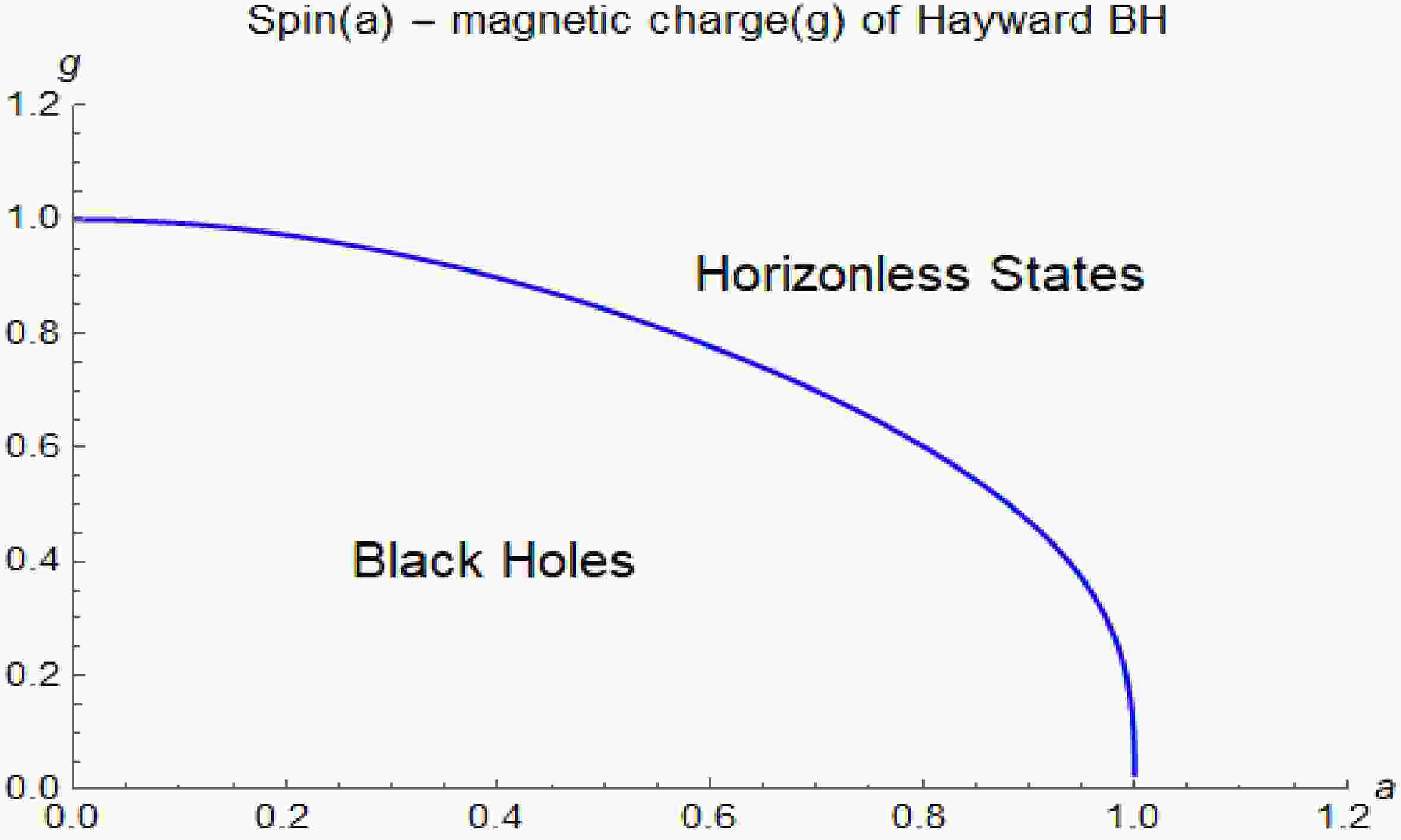
$ \Delta=0 $ , which sets constraints on the spin and magnetic charge parameters of the BH. Beyond these limits, the BH transitions to a horizonless state; this regime has not been considered in the present study. These parameters are further restricted by observational and theoretical considerations: the spin parameter cannot exceed the Chandrasekhar limit, and the magnetic charge is limited to$ g \leqslant 1.72 $ , in agreement with the observational data (obtained from M87*) within the 1σ confidence interval [66]. Figure 1 depicts the viable parameter space for rotating Hayward BHs, highlighting configurations that sustain an event horizon. The inverse metric$ g^{\mu\nu} $ provides the starting point for constructing the Christoffel symbols of the Hayward spacetime. They are defined by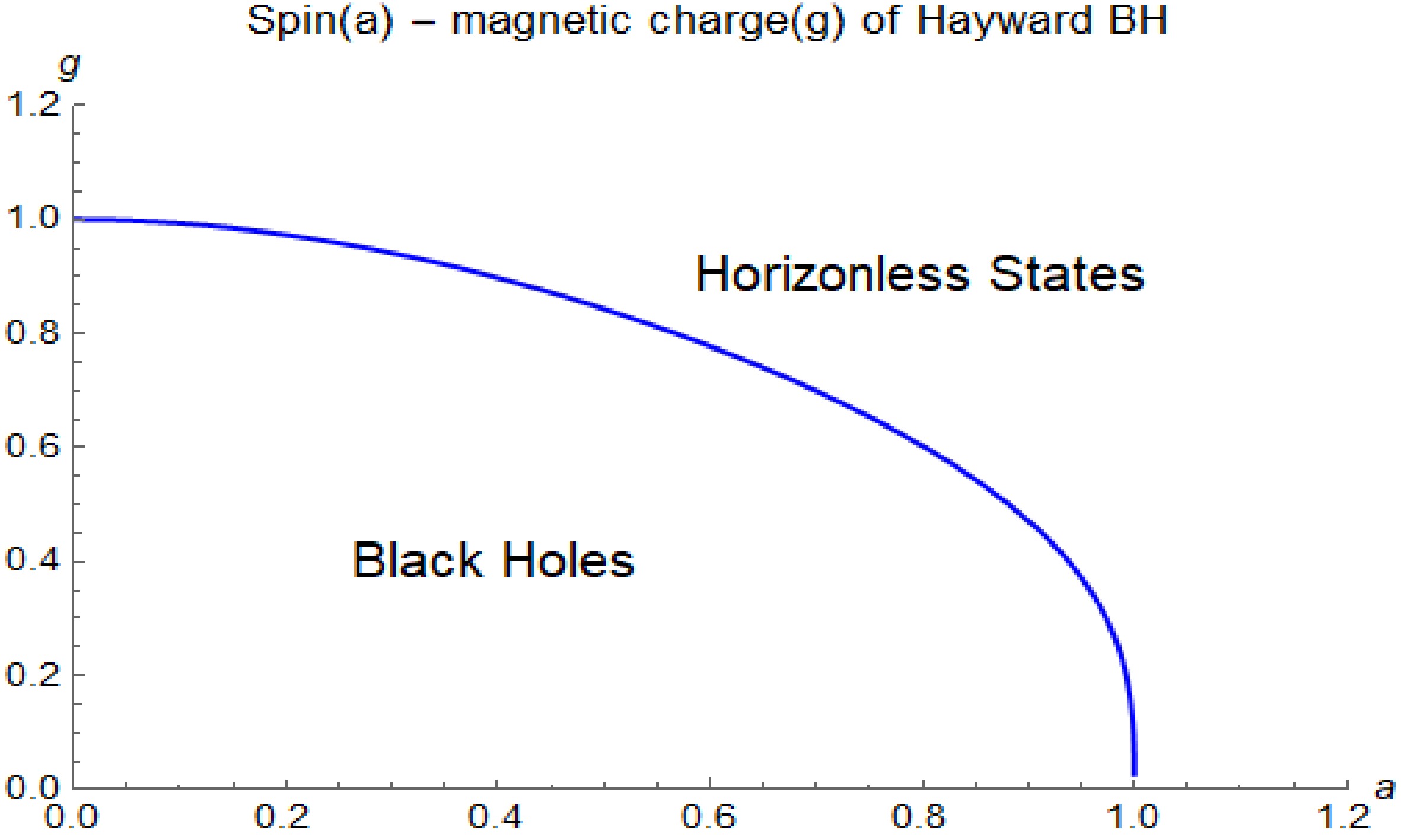
Figure 1. (color online) Parameter space in terms of (
$a,g$ ) is shown, delineating regions associated with BHs and horizonless spacetimes. Configurations enclosed within the blue boundary represent BHs with an event horizon, whereas regions outside this boundary correspond to horizonless spacetimes.$ \Gamma^{\alpha}{}_{\mu\nu} = \dfrac{1}{2}\, g^{\alpha s} \bigl(\partial_{\mu} g_{\nu s} + \partial_{\nu} g_{\mu s} - \partial_{s} g_{\mu\nu}\bigr). $
(4) Photon dynamics are described within the Hamiltonian framework, where the Hamiltonian reads
$ H = \dfrac{1}{2}\, g^{\mu\nu} p_\mu p_\nu, $
(5) with
$ p_\mu $ the photon's covariant four-momentum. For massless particles,$ H=0 $ . Restricting to equatorial motion ($ \theta=\pi/2 $ ) and using the conserved quantities$ E=-p_t $ and$ L=p_\phi $ , the Hamiltonian becomes$ H(r, p_r; E, L) = g^{tt} E^2 + 2 g^{t\phi} E L + g^{\phi\phi} L^2 + g^{rr} p_r^2, $
(6) leading to the effective potential
$ R(r) \equiv g^{rr} p_r^2 = -\Big( g^{tt} E^2 + 2 g^{t\phi} E L + g^{\phi\phi} L^2 \Big), $
(7) with
$ R(r) \geqslant 0 $ for allowed photon motion. Circular photon orbits satisfy$ R(r)=0, \qquad \dfrac{{\rm d}R(r)}{{\rm d}r}=0, $
(8) which determine
$ (E,L) $ and the stability regime of photon orbits [48, 67].For a more practical form of orbital integrals, one converts to the contravariant four-momentum,
$ p^\mu = g^{\mu\nu} p_\nu, $ which corresponds physically to the photon's four-velocity,$ U^\mu = \left(\dfrac{{\rm d}t}{{\rm d}\lambda},\, \dfrac{{\rm d}r}{{\rm d}\lambda},\, \dfrac{{\rm d}\theta}{{\rm d}\lambda},\, \dfrac{{\rm d}\phi}{{\rm d}\lambda}\right), $
(9) which serves as the initial condition for numerical integration.
The geodesic and polarization parallel-transport equations can be written as a first-order ODE system:
$ \dfrac{{\rm d}x^\mu}{{\rm d}\lambda}=k^\mu, \qquad \dfrac{{\rm d}k^\mu}{{\rm d}\lambda}=-\Gamma^{\mu}{}_{\nu\rho} k^\nu k^\rho, $
(10) $ \dfrac{{\rm d}f^\mu}{{\rm d}\lambda}+\Gamma^{\mu}{}_{\nu\rho} k^\nu f^\rho=0, $
(11) where
$ k^\mu $ is the photon four-momentum and$ f^\mu $ the polarization vector. Eq. (11) can be equivalently written as$ \dfrac{{\rm d}f^\mu}{{\rm d}\lambda}=-\Gamma^{\mu}{}_{\nu\rho}\,k^\nu f^\rho. $
(12) To construct a closed ODE system, we proceed as follows: (1) Introduce the conserved quantities,
$ p_t=-E, p_\phi=L $ associated with stationarity and axisymmetry; (2) Express all dynamical variables explicitly as functions of the affine parameter λ, e.g.,$ r \mapsto r(\lambda),\quad \theta \mapsto \theta(\lambda), f^t \mapsto f^t(\lambda),\quad p_r \mapsto p_r(\lambda). $ ; (3) Combine the geodesic and polarization transport equations into the coupled system$ \dfrac{{\rm d}t}{{\rm d}\lambda} = k^t, \dfrac{{\rm d}r}{{\rm d}\lambda} = k^r, $
(13) $ \dfrac{{\rm d}\theta}{{\rm d}\lambda} = k^\theta, \dfrac{{\rm d}\phi}{{\rm d}\lambda} = k^\phi, $
(14) $ \dfrac{{\rm d}k^\mu}{{\rm d}\lambda} = -\Gamma^{\mu}{}_{\nu\rho}\,k^\nu k^\rho, $
(15) $ \dfrac{{\rm d}f^\mu}{{\rm d}\lambda} = -\Gamma^{\mu}{}_{\nu\rho}\,k^\nu f^\rho, $
(16) This formulation yields 10 first-order ordinary differential equations (ODEs) in total: (i) six equations for the geodesic variables
$ \{t', r', \theta', \phi', p_r', p_\theta'\} $ ; (ii) four equations for the polarization components$ \{f^t, f^r, f^\theta, f^\phi\} $ . Accordingly, the general-relativistic polarized radiation transfer problem reduces to a closed ODE system. With appropriate initial conditions, an ODE solver can simultaneously evolve both photon trajectories and polarization states, providing the foundation for subsequent radiative transfer calculations and polarization image synthesis. -
In this section, we provide a succinct overview of rotating Hayward BHs and examine the motion characteristics of particles within the corresponding spacetime. The metric describing a rotating Hayward BH is expressed as follows [64]:
$ \begin{aligned}[b] {\rm{d}}s^2 = &- \left(1 - \dfrac{2 m(r) r}{\sum} \right) {\rm{d}} t^2 - \dfrac{4 a m(r) r}{\sum} \sin^{2}\theta {\rm{d}} t {\rm{d}} \phi + \dfrac{\sum}{\Delta} {\rm{d}} r^2\\ & + \sum {\rm{d}} \theta^{2} + \left(r^2 + a^2 +\dfrac{2 m(r) r a^2 \sin^{2}\theta}{\sum} \right) \sin^{2}\theta {\rm{d}} \phi^{2},\end{aligned} $
(1) where
$ \sum = r^{2} + a^{2}\cos^{2}\theta,\; \; \; \; \; \; \Delta = r^{2} + a^{2} - 2 m(r) r. $
(2) Here,
$ m(r) $ represents the mass function, defined as [65]$ m(r) = \dfrac{M r^3}{r^3 + g^3}, $
(3) where a denotes the BH spin, and g is the magnetic charge. In the limiting case
$ g \rightarrow 0 $ , the rotating Hayward BH reduces to the Kerr BH, thereby encapsulating the causal structure of the Kerr spacetime within the framework of the rotating Hayward BH.The event horizon of a rotating Hayward BH is defined by the largest root of the equation
$ \Delta=0 $ , which sets constraints on the spin and magnetic charge parameters of the BH. Beyond these limits, the BH transitions to a horizonless state; this regime has not been considered in the present study. These parameters are further restricted by observational and theoretical considerations: the spin parameter cannot exceed the Chandrasekhar limit, and the magnetic charge is limited to$ g \leqslant 1.72 $ , in agreement with the observational data (obtained from M87*) within the 1σ confidence interval [66]. Figure 1 depicts the viable parameter space for rotating Hayward BHs, highlighting configurations that sustain an event horizon. The inverse metric$ g^{\mu\nu} $ provides the starting point for constructing the Christoffel symbols of the Hayward spacetime. They are defined by
Figure 1. (color online) Parameter space in terms of (
$a,g$ ) is shown, delineating regions associated with BHs and horizonless spacetimes. Configurations enclosed within the blue boundary represent BHs with an event horizon, whereas regions outside this boundary correspond to horizonless spacetimes.$ \Gamma^{\alpha}{}_{\mu\nu} = \dfrac{1}{2}\, g^{\alpha s} \bigl(\partial_{\mu} g_{\nu s} + \partial_{\nu} g_{\mu s} - \partial_{s} g_{\mu\nu}\bigr). $
(4) Photon dynamics are described within the Hamiltonian framework, where the Hamiltonian reads
$ H = \dfrac{1}{2}\, g^{\mu\nu} p_\mu p_\nu, $
(5) with
$ p_\mu $ the photon's covariant four-momentum. For massless particles,$ H=0 $ . Restricting to equatorial motion ($ \theta=\pi/2 $ ) and using the conserved quantities$ E=-p_t $ and$ L=p_\phi $ , the Hamiltonian becomes$ H(r, p_r; E, L) = g^{tt} E^2 + 2 g^{t\phi} E L + g^{\phi\phi} L^2 + g^{rr} p_r^2, $
(6) leading to the effective potential
$ R(r) \equiv g^{rr} p_r^2 = -\Big( g^{tt} E^2 + 2 g^{t\phi} E L + g^{\phi\phi} L^2 \Big), $
(7) with
$ R(r) \geqslant 0 $ for allowed photon motion. Circular photon orbits satisfy$ R(r)=0, \qquad \dfrac{{\rm d}R(r)}{{\rm d}r}=0, $
(8) which determine
$ (E,L) $ and the stability regime of photon orbits [48, 67].For a more practical form of orbital integrals, one converts to the contravariant four-momentum,
$ p^\mu = g^{\mu\nu} p_\nu, $ which corresponds physically to the photon's four-velocity,$ U^\mu = \left(\dfrac{{\rm d}t}{{\rm d}\lambda},\, \dfrac{{\rm d}r}{{\rm d}\lambda},\, \dfrac{{\rm d}\theta}{{\rm d}\lambda},\, \dfrac{{\rm d}\phi}{{\rm d}\lambda}\right), $
(9) which serves as the initial condition for numerical integration.
The geodesic and polarization parallel-transport equations can be written as a first-order ODE system:
$ \dfrac{{\rm d}x^\mu}{{\rm d}\lambda}=k^\mu, \qquad \dfrac{{\rm d}k^\mu}{{\rm d}\lambda}=-\Gamma^{\mu}{}_{\nu\rho} k^\nu k^\rho, $
(10) $ \dfrac{{\rm d}f^\mu}{{\rm d}\lambda}+\Gamma^{\mu}{}_{\nu\rho} k^\nu f^\rho=0, $
(11) where
$ k^\mu $ is the photon four-momentum and$ f^\mu $ the polarization vector. Eq. (11) can be equivalently written as$ \dfrac{{\rm d}f^\mu}{{\rm d}\lambda}=-\Gamma^{\mu}{}_{\nu\rho}\,k^\nu f^\rho. $
(12) To construct a closed ODE system, we proceed as follows: (1) Introduce the conserved quantities,
$ p_t=-E, p_\phi=L $ associated with stationarity and axisymmetry; (2) Express all dynamical variables explicitly as functions of the affine parameter λ, e.g.,$ r \mapsto r(\lambda),\quad \theta \mapsto \theta(\lambda), f^t \mapsto f^t(\lambda),\quad p_r \mapsto p_r(\lambda). $ ; (3) Combine the geodesic and polarization transport equations into the coupled system$ \dfrac{{\rm d}t}{{\rm d}\lambda} = k^t, \dfrac{{\rm d}r}{{\rm d}\lambda} = k^r, $
(13) $ \dfrac{{\rm d}\theta}{{\rm d}\lambda} = k^\theta, \dfrac{{\rm d}\phi}{{\rm d}\lambda} = k^\phi, $
(14) $ \dfrac{{\rm d}k^\mu}{{\rm d}\lambda} = -\Gamma^{\mu}{}_{\nu\rho}\,k^\nu k^\rho, $
(15) $ \dfrac{{\rm d}f^\mu}{{\rm d}\lambda} = -\Gamma^{\mu}{}_{\nu\rho}\,k^\nu f^\rho, $
(16) This formulation yields 10 first-order ordinary differential equations (ODEs) in total: (i) six equations for the geodesic variables
$ \{t', r', \theta', \phi', p_r', p_\theta'\} $ ; (ii) four equations for the polarization components$ \{f^t, f^r, f^\theta, f^\phi\} $ . Accordingly, the general-relativistic polarized radiation transfer problem reduces to a closed ODE system. With appropriate initial conditions, an ODE solver can simultaneously evolve both photon trajectories and polarization states, providing the foundation for subsequent radiative transfer calculations and polarization image synthesis. -
With the ODE system for geodesic motion and polarization transport, we perform ray-tracing calculations. To ensure numerical stability and physical consistency, we normalize both the metric inputs and polarization angles such that the polarization directions remain consistent throughout propagation, avoiding artifacts from numerical discontinuities. We first determine the Hayward metric in Eq. (1), which yields the covariant tensor
$ g_{\mu\nu} $ used as an input for ray tracing. During photon propagation, both azimuthal angle differences and polarization angles are normalized. Accordingly, we define a normalization function$ F[a_1,a_2] $ that maps the angles to the standard ranges$ a_1 \mapsto [0,2\pi) $ and$ a_2 \mapsto [0,\pi) $ . In practice, this mapping is implemented as$ \{x_1, x_2\} = F[a_1, a_2]. $
(17) Here,
$ x_1 $ represents the azimuthal angle difference, and$ x_2 $ is the polarization angle. Physically, this normalization enforces the identification$ \theta \sim \theta+\pi $ [68]. When$ x_1<0 $ , we reflect the azimuthal difference and rotate the polarization by π to maintain directional consistency:$ x_1 \to -x_1 $ ,$ x_2 \to x_2+\pi $ , followed by reducing$ x_2 $ modulo$ 2\pi $ . The final normalized pair is$ \{x_1, x_2\} = \left( |a_1|,\ (a_2 + \pi\,\delta_{a_1<0}) \text{mod} 2\pi \right), $
(18) where
$ \delta_{a_1<0}=1 $ if$ a_1<0 $ and$ 0 $ otherwise.To relate ray-tracing results to observational quantities, we introduce local orthonormal tetrads in curved spacetime. This formalism defines physical quantities such as energy, angular momentum, and polarization angles in the instantaneous rest frame of a local observer. The orthonormal basis
$ \{e_{(0)}, e_{(1)}, e_{(2)}, e_{(3)}\} $ satisfies$ \eta_{ab}=\mathrm{diag}(-1,\,1,\,1,\,1), \qquad g_{\mu\nu}\, e^\mu_{(a)} e^\nu_{(b)} = \eta_{ab}. $
(19) Here,
$ \eta_{ab} $ is the Minkowski metric. This basis is then used to project photon momenta and polarization vectors into the observers frame [69].●
$ e^\mu_{(0)} $ (observer/ZAMO four-velocity, including frame dragging):$ e^\mu_{(0)} = \sqrt{\dfrac{-\,g_{\phi\phi}}{\,g_{tt} g_{\phi\phi} - g_{t\phi}^2\,}} \left(1,\,0,\,0,\,-\dfrac{g_{t\phi}}{g_{\phi\phi}}\right), $
(20) satisfying
$ g_{\mu\nu} e^\mu_{(0)} e^\nu_{(0)}=-1 $ .●
$ e^\mu_{(1)} $ (radial unit vector):$ e^\mu_{(1)}=\left(0,\,-\dfrac{1}{\sqrt{g_{rr}}},\,0,\,0\right). $
(21) ●
$ e^\mu_{(2)} $ (polar unit vector) and$ e^\mu_{(3)} $ (azimuthal unit vector):$ e^\mu_{(2)}=\left(0,\,0,\,\dfrac{1}{\sqrt{g_{\theta\theta}}},\,0\right),\qquad e^\mu_{(3)}=\left(0,\,0,\,0,\,-\dfrac{1}{\sqrt{g_{\phi\phi}}}\right). $
(22) Together, these vectors form the local orthonormal basis required to extract observational quantities such as photon energy, redshift, and polarization angles.
Next, we relate image-plane coordinates to normalized field-of-view (FOV) coordinates. For pixel indices
$ (i,j)\in[1, \cdots ,N_{\rm pix}] $ , we map to normalized screen coordinates$ (x_{\rm scr},y_{\rm scr}) = \dfrac{2 \tan ({\rm fov}/2)}{N_{\rm pix}} \left(i - \dfrac{1}{2}(N_{\rm pix}+1), j - \dfrac{1}{2}(N_{\rm pix}+1)\right), $
(23) where FOV is the field-of-view angle. This mapping centers the image at
$ (0,0) $ and normalizes the coordinates to the range$ [-\tan({\rm fov}/2),\tan({\rm fov}/2)] $ [70]. These coordinates are then converted to spherical direction angles via$ \{\theta_{x}, \psi_{x} \} = F \left(2 \arctan \left(\dfrac{1}{2}\sqrt{x_{\rm scr}^{2} + y_{\rm scr}^{2}}\right), \arctan \dfrac{y_{\rm scr}}{x_{\rm scr}}\right). $
(24) The normalization function F ensures consistency of the polarization alignment with photon propagation. From these angles we construct the 3D propagation direction in the local observers frame:
$ \vec{v}=\bigl(\cos\theta_x,\, \sin\theta_x\cos\psi_x,\, \sin\theta_x\sin\psi_x\bigr). $
(25) Finally, the photons initial four-momentum is
$ \lambda^\mu = -\kappa\, e^\mu_{(0)} + v^{(1)} e^\mu_{(1)} + v^{(2)} e^\mu_{(2)} + v^{(3)} e^\mu_{(3)}, $
(26) where κ is a normalization constant (typically set to unity) and
$ \vec{v}=(v^{(1)},v^{(2)},v^{(3)}) $ is the propagation direction vector. This construction ensures$ \lambda^\mu \lambda_\mu=0 $ , confirming that the four-momentum is null and providing the boundary condition for subsequent ray-tracing calculations. -
With the previous framework in place, we now focus on constructing BH images through radiative transfer calculations. This process requires a physically motivated prescription for the background emission source, which is characterized by the source function intensity
$ I(r) $ at the radial coordinate r [71]. The intensity profile defines the initial photon flux along each geodesic and thus plays a fundamental role in image formation. For example, it could represent emission from an accretion disk or a hot corona, serve as the initial source term in ray tracing, and provide a simplified version of the emission function$ j(\nu, r) $ in the radiative transfer equation.A frequently adopted model is the Gaussian-type intensity profile, which is smooth and devoid of singularities, thus preventing numerical instabilities near its peak. In realistic astrophysical contexts, however, radiation from accretion flows, jets, and coronae often exhibits pronounced asymmetry and intricate spatial morphology. To capture such behaviors, we employ a more flexible, non-Gaussian intensity distribution function [72].
$ I(r)=\left(1+\alpha \tanh (\gamma x)\right)\cdot \dfrac{\exp\left[-\dfrac{1}{2}\left(\sinh^{-1}(x)\right)^2\right]}{\left(x^2+1\right)^{\delta/2}}, \quad x=\dfrac{r-\beta}{\sigma }. $
(27) In this expression, the normalized radial coordinate x is defined with a scaling factor σ; the term
$ \tanh(\gamma x) $ serves to introduce an adjustable asymmetry; the exponential component produces a smooth central peak; and the power-law component regulates the decay of the tail. The physical interpretations and default settings of the parameters in the intensity distribution function are as follows: r denotes the radial coordinate (no default value); β specifies the peak position of the intensity profile (default: 6); σ serves as the width parameter that defines the spatial extent of the profile (default: 1); γ controls the degree of asymmetry (default: 0); δ represents the tail-decay exponent governing the convergence rate at large distances (default: 1); and α determines the amplitude of asymmetry (default: 0.5). Collectively, these parameters shape and characterize the overall form of the intensity distribution.According to the model, when
$ \gamma \gt 0 $ , the intensity is enhanced in the region$ r \gt \beta $ ; conversely, for$ \gamma \lt 0 $ , the emission is stronger at$ r \lt \beta $ . The parameter α controls the degree of asymmetry in the profile. The exponential component ensures smooth behavior near the center, while the power-law tail term represents extended disk-like emission: larger values of$ \delta \gt 1 $ cause faster intensity decay (short-range emission), whereas smaller values of$ \delta \lt 1 $ produce broader, more extended profiles. -
In scenarios involving polarized radiation, the observed intensity depends not only on the radial emission profile but also on the relative orientation between the polarization vector and the observers line of sight. A straightforward treatment applies an angular modulation with a cosine dependence:
$ I_{\rm pol}(r, \theta) \propto \cos^2 \theta, $
(28) where θ denotes the angle between the polarization direction and the line of sight. This modulation encapsulates the anisotropic nature of polarized emission and parallels the behavior observed in synchrotron radiation and Rayleigh/Thomson scattering. For example, when
$ \theta = \pi/3 $ , one obtains$ \cos^2(\pi/3) = 1/4 $ , implying that the polarized intensity is reduced to one quarter of its maximum value.Extending the unpolarized intensity profile
$ I(r) $ , we incorporate a Gaussian-like kernel with an appropriate normalization factor to establish a fundamental model of polarized emissivity [73]:$ {I_{\rm pol}(r) = \cos^2\theta \cdot \dfrac{1}{2\sqrt{(r-\beta)^2 + \sigma ^2}} \exp\left[ -\dfrac{1}{2} \left( \gamma + \sinh^{-1}\left( \dfrac{r - \beta}{\sigma } \right) \right)^2 \right]. }$
(29) Here, the
$ \cos^2\theta $ term introduces angular modulation due to polarization, while the exponential factor ensures a smooth radial intensity profile. This expression can be interpreted as a polarized extension of$ I(r) $ , where the$ \cos^2\theta $ term accounts for the selection effect arising from polarization geometry. The Gaussian-like kernel yields a peaked intensity structure, the normalization term guarantees proper decay at large radii r, and the angular factor encapsulates the intrinsic directional sensitivity of polarized emission mechanisms.While the model proves useful for simplified analysis, it is still an idealized representation. The single
$ \cos^2\theta $ term overlooks complex angular behaviors that may occur in magnetized or anisotropic media. The Gaussian-like profile is symmetric by nature〞although γ introduces minor asymmetry, it fails to describe the full irregularities observed in turbulent or strongly anisotropic environments. Additionally, its lack of frequency dependence limits the description of interactions between spectral and polarization features.In more realistic astrophysical environments, the polarized emissivity is a function not only of the radial coordinate r but also of the viewing angle θ, the observing frequency ν, the polarization degree Π, and any inherent asymmetry. Introducing the dimensionless parameter
$ x = \dfrac{r - \beta}{\sigma }, $
(30) we can express a generalized polarized source function [74] as
$ \begin{aligned}[b]I_p(r, \theta, \nu) = &\Pi \cdot \cos^2\theta \cdot \left( \dfrac{\nu^3}{{\rm e}^{\nu / T(r)} - 1} \right) \cdot\\ &(1 + \alpha \tanh(\gamma x)) \cdot \dfrac{\exp\left[ -\dfrac{1}{2} (\sinh^{-1} x)^2 \right]}{(x^2 + 1)^{\delta / 2}}. \end{aligned} $
(31) This expression simultaneously incorporates multiple physical factors: angular dependence (
$ \cos^2\theta $ ), polarization degree (II), spectral dependence through a Planck-like factor, asymmetry via$ (1 + \alpha \tanh(\gamma x)) $ , and a spatial kernel characterized by a power-law tail. The Gaussian-like exponential term ensures spatial localization, while the decay index δ governs the falloff at large radii. The asymmetry factor introduces deviations from strict radial symmetry, capturing realistic conditions found in turbulent plasmas, magnetized disks, and jetCdisk interaction regions.Compared with Eq. (28), this generalized formulation offers greater flexibility. It incorporates frequency dependence, allowing analysis of spectralCpolarization coupling; the asymmetry parameters
$ (\alpha, \gamma) $ account for leftCright brightness modulation; and the decay index δ provides tunable control over the tail behavior. These enhancements enable the model to describe a broader class of astrophysical environments, including relativistic jets, magnetized coronae, and accretion flows with limb brightening. -
To explore how spacetime geometry shapes polarization patterns, we consider a set of spatially uniform magnetic fields embedded in the KerrCNewman spacetime. In the local ZAMO orthonormal tetrad
$ \{e_{(0)}, e_{(1)}, e_{(2)}, e_{(3)}\} $ , the magnetic field takes the form:$ B^\mu = (0, B^{(1)}, B^{(2)}, B^{(3)}), $
(32) with the components corresponding to the radial, polar, and azimuthal directions, respectively. For optically thin synchrotron emission, the polarization degree is expressed as
$ \Pi_{\rm syn} = \dfrac{p + 1}{p + 7/3} $ , where p denotes the electron energy index. The electric vector is orthogonal to the projected magnetic field$ {\bf{B}}_\perp $ . The screen-projection operator in the tetrad frame is:$ h^\mu_{\,\,\nu} = \delta^\mu_{\,\,\nu} + e^\mu_{\,(0)} e_{(0)\,\nu}, \quad B^\mu_\perp = h^\mu_{\,\,\nu} B^\nu, $
(33) and the local electric vector position angle (EVPA) satisfies
$ \psi = \arg \left( B^{(1)}_\perp + {\rm i} B^{(2)}_\perp \right) + \dfrac{\pi}{2}, \quad \tan(2\chi) = \dfrac{U}{Q}, $
(34) where
$ Q = \Pi_{\rm syn} I \cos 2\chi $ and$ U = \Pi_{\rm syn} I \sin 2\chi $ . In the absence of Faraday rotation, the EVPA is parallel transported along null geodesics to the observers image plane, producing the observable polarization distribution.We analyze four representative constant magnetic field configurations, which serve as benchmarks for interpreting polarization morphologies:
(i) Pure radial field (
$ B^\mu = (0, 1, 0, 0) $ ): Polarization vectors exhibit concentric, ring-like patterns consistent with the$ E \perp B $ projection. Near the photon ring, strong lensing and frame dragging enhance shear distortions [75].(ii) Pure polar field (
$ B^\mu = (0, 0, 1, 0) $ ): The projected field is inclined in the image plane, giving rise to a vortex-like EVPA twist. The sense of rotation (clockwise or counterclockwise) depends on the BH spin and observer inclination [76].(iii) Pure azimuthal (toroidal) field (
$ B^\mu = (0, 0, 0, 1) $ ): The projected component$ B_\perp $ appears nearly radial, producing radially oriented electric vectors. Higher-order photon trajectories near the photon ring lead to azimuthal periodic modulation [41].(iv) Mixed radialCpolar field (
$ B^\mu = (0, 0.87, 0.5, 0) $ ): The combination of radial and polar components forms an open spiral EVPA structure. The spiral pitch and arm width depend on the ratio$ B^{(1)}/B^{(2)} $ , consistent with polar-dominated configurations such as those inferred for M87* [40].Horizon-scale polarimetric imaging of BHs (e.g., M87* and Sgr A*) and GRMHD simulations consistently show that differential rotation within the inner accretion flow winds large-scale poloidal magnetic flux into a toroidally dominated structure, generating helical fields near the jet-launching region [58]. Frame dragging in Hayward spacetimes further twists field lines, altering their pitch angles via relativistic aberration and gravitational lensing. Guided by this astrophysical scenario, we adopt simple, tunable models for helical magnetic fields that capture the essential geometric features while remaining analytically tractable for polarized radiative transfer. In the ZAMO orthonormal tetrad
$ \{e_{(0)}, e_{(1)}, e_{(2)}, e_{(3)}\} $ , the magnetic field is defined as$ B^\mu(r) = (0, B^r(r), B^\theta(r), B^\phi(r)) $ , where the spatial components correspond to the radial, polar, and azimuthal directions, respectively.For optically thin synchrotron radiation produced by a power-law electron distribution
$ N(E) \propto E^{-p} $ with spectral index$ \alpha = (p - 1)/2 $ , the maximum intrinsic polarization fraction is:$ \Pi_0 = \dfrac{\alpha + 1}{\alpha + \dfrac{5}{3}} \quad ({\rm typically} \; \; \; 70\%-75\%). $
(35) Defining the screen projection operator
$h^\mu_{\,\,\nu} = \delta^\mu_{\,\,\nu} + e^\mu_{\,(0)} e_{(0)\,\nu}$ , the projected magnetic field becomes$B^\mu_\perp = h^\mu_{\,\,\nu} B^\nu$ . The corresponding EVPA is given by Eq. (33), with the emissivities defined as$ j_I \propto |B_\perp|^{\alpha + 1}, \quad j_Q = \Pi_0 j_I \cos(2\chi), \quad j_U = \Pi_0 j_I \sin(2\chi). $
(36) Without Faraday rotation, ψ is parallel-transported along null geodesics, whereas relativistic lensing and frame dragging generate distinctive shear and twist patterns in the polarization near the photon ring. To capture a wide range of morphologies efficiently, we implement logarithmic-radius modulations that allow control over the twist frequency. A straightforward and physically well-justified astrophysical choice is
$\begin{aligned}[b] &B^r(r) = \dfrac{b_{\rm ratio}}{r}, \quad B^\theta(r) = \dfrac{amp}{r} \sin(k \ln r),\\ & B^\phi(r) = \dfrac{1}{r} \left[1 + \dfrac{1}{2} \cos(k \ln r)\right]. \end{aligned}$
(37) In this parameterization, k denotes the twist frequency per unit
$ \ln r $ , thereby determining the number of helical turns per radial decade. The coefficient$ amp $ sets the amplitude of the vertical undulation, and$ b_{\rm ratio} $ controls the strength of the radial opening. Toroidal component$ B^\phi $ remains dominant in both cases, consistent with magnetic flux winding in GRMHD simulations of magnetically arrested disks. The local pitch angle is conveniently defined as$ \tan \psi(r) = \dfrac{\sqrt{[B^r(r)]^2 + [B^\theta(r)]^2}}{B^\phi(r)}. $
(38) An increase in either
$ b_{\rm ratio} $ or$ amp $ broadens the spiral pattern, corresponding to a larger pitch angle ψ, whereas increasing k enhances the number of windings per radial decade without substantially altering the local opening angle. Magnetic streamlines are obtained by integrating in spherical coordinates$ (r, \theta, \phi) $ :$ \dfrac{{\rm d}r}{{\rm d}s} = B^r(r), \qquad \dfrac{{\rm d}\theta}{{\rm d}s} = \dfrac{B^\theta(r)}{r}, \qquad \dfrac{{\rm d}\phi}{{\rm d}s} = \dfrac{B^\phi(r)}{r \sin\theta}, $
(39) and subsequently mapped to Cartesian coordinates
$ (x, y, z) = (r \sin\theta \cos\phi,\, r \sin\theta \sin\phi,\, r \cos\theta) $ . These trajectories visualize the geometrical roles of$ (k, amp, b_{\rm ratio}) $ and aid in interpreting the polarization morphologies derived from Eqs. (36).For an equatorial viewing geometry, where the image-plane axes satisfy
$ x \parallel \phi $ and$ y \parallel \theta $ , the projected field components obey$ (B_x, B_y) \simeq (B^\phi, B^\theta) $ . The local EVPA is then approximated by$ \chi(r) \approx \dfrac{1}{2} \arctan \left(\dfrac{B_y}{B_x}\right) + \dfrac{\pi}{2} = \dfrac{1}{2} \arctan \left(\dfrac{B^\theta(r)}{B^\phi(r)}\right) + \dfrac{\pi}{2}. $
(40) The radial dependence of
$ \chi(r) $ reflects the magnetic twist introduced by the parameter k. When the toroidal component dominates ($ B^\phi \gg B^r, B^\theta $ ), EVPAs align radially; the inclusion of$ B^\theta $ and$ B^r $ generates spiral polarization patterns with pitch governed by Eq. (38). Near the photon ring, multiple imaging and parallel transport produce characteristic sign changes in$ Q/U $ and swirling EVPA structures, both amplified by increasing the BH spin and observer inclination. -
With the helical magnetic field defined at each spacetime point, we set up the initial polarization state needed for general-relativistic polarized radiative transfer. For an emission event at position
$ x^\mu $ with photon four-momentum$ k^\mu $ ($ k^\mu k_\mu = 0 $ ), polarization four-vector$ f^\mu $ must satisfy$ transversality: \quad k_\mu f^\mu = 0, $
(41) $ normalization: \quad f^\mu f_\mu = \pm 1, $
(42) where the sign depends on the chosen metric signature (here
$ (-, +, +, +) $ ). Denoting the observers four-velocity by$ U^\mu $ (ZAMO) and the magnetic field by$ B^\mu $ , we define the polarization vector covariantly as$ f^\mu \propto \varepsilon^{\mu\nu\rho\sigma } U_\nu k_\rho B_\sigma , $
(43) motivated by the orthogonality between the EVPA and the projected magnetic field in optically thin synchrotron radiation. Since
$ \varepsilon^{\mu\nu\rho\sigma } $ is totally antisymmetric, the transversality condition holds automatically:$ k_\mu f^\mu \propto \varepsilon_{\mu\nu\rho\sigma } k^\mu U^\nu k^\rho B^\sigma = 0, $
(44) which ensures the transversality condition (Eq. (40)). Furthermore, due to the antisymmetry of
$ \varepsilon^{\mu\nu\rho\sigma } $ , one finds$ U_\mu f^\mu = 0 $ , implying that$ f^\mu $ resides entirely in the local three-space orthogonal to the observers four-velocity. Geometrically, Eq. (42) corresponds to the Hodge dual of the oriented three-volume defined by$ (U^\mu, k^\mu, B^\mu) $ ; within the observers screen, it points perpendicular to the projected magnetic field$ {\bf{B}}_\perp $ , reproducing the synchrotron relation$ E \perp B_\perp $ . Applying the normalization constraint (Eq. (41)) yields$ f^\mu = \dfrac{\varepsilon^{\mu\nu\rho\sigma } U_\nu k_\rho B_\sigma }{\sqrt{\left| (\varepsilon^{\alpha\beta\gamma\delta} U_\beta k_\gamma B_\delta)g_{\alpha\lambda}(\varepsilon^{\lambda\eta\kappa\xi} U_\eta k_\kappa B_\xi)\right|}}. $
(45) This definition is explicitly covariant and coordinate-independent, and up to the standard gauge freedom
$ f^\mu \rightarrow f^\mu + a k^\mu $ is equivalent to a GramCSchmidt orthogonalization in the screen subspace. In the flat spacetime limit ($ U^\mu = (1, {\bf{0}}) $ ),$ f^\mu $ reduces to a spatial unit vector orthogonal to the plane spanned by$ {\bf{k}} $ and$ {\bf{B}} $ .When Faraday effects are neglected, the polarization four-vector is parallel-transported along the null geodesic toward the observer. Projection of
$ f^\mu $ onto the image-plane tetrad$ \{e_{(1)}, e_{(2)}\} $ yields$ f^{(i)} = f^\mu e^{(i)}_\mu $ , from which the EVPA follows as$ \chi = \dfrac{1}{2}\,{\rm atan}2(f^{(2)}, f^{(1)}), $
(46) where
$ {\rm atan}2 $ guarantees the correct angular quadrant. The polarization fraction Π is specified by the emissivity model [Eqs. (26), (30)], and the Stokes parameters are then$ Q = \Pi I \cos 2\chi, \qquad U = \Pi I \sin 2\chi. $
(47) where I represents the total intensity. When Faraday rotation and conversion are non-negligible, the complete Stokes vector
$ (I, Q, U, V) $ must be evolved along the null geodesic according to the covariant polarized radiative transfer equation. Equation (14) explicitly demonstrates that the observed polarization is determined by the geometric relation among the photon propagation direction, the local magnetic field, and the observers rest frame. In curved spacetime, parallel transport of$ f^\mu $ encodes the effects of frame dragging and gravitational lensing, giving rise to shear and twist of EVPAs near critical curves such as photon rings. Multiple imaging may further generate sign changes in$ Q/U $ . In conjunction with the helical magnetic field prescriptions of Eq. (36), this construction provides a direct and observationally testable connection between magnetized accretion geometry and horizon-scale polarization structure. -
In the preceding section, we presented the simulation results of a rotating Hayward BH surrounded by a thin accretion disk. Observational data from the EHT further demonstrate that polarimetric imaging of BHs, such as M87* and the supermassive BH at the center of the Milky Way, can reveal polarization information in their immediate vicinity [40–41, 43, 77]. Notably, strong linear polarization is observed from synchrotron emission at an observational wavelength of
$ 1.3 $ mm [40–41].The polarization state propagates through a magnetized plasma, undergoing Faraday rotation and transformation. Due to the complex interplay between emission and propagation effects, numerical radiative transfer calculations are crucial for accurately capturing the observed polarization of M87* and Sgr A*. In addition to the intensity component (Stokes
$ {\cal{I}} $ ), ray-tracing techniques can be employed to determine the observed linear polarization (Stokes$ {\cal{P}} = {\cal{Q}} + i {\cal{U}} $ ) and generate polarization images, as demonstrated in previous studies [78–79].Unlike in Euclidean space, the transport of a tensor along a manifold is path-dependent, requiring a consistent set of propagation rules to preserve “directional” invariance. Given a curve
$ {\cal{C}} $ on the manifold$ {\cal{M}} $ , with tangent vectors$ t^{\rm{u}} $ at each point, a tensor$ T^{\rho_1 \cdots \rho_k}_{\sigma _1 \cdots \sigma _l} $ remains covariant along$ {\cal{C}} $ if$ t^{ \mu} \nabla_{ \mu} T^{\rho_{1}\cdot\cdot\cdot\rho_{k}}_{\sigma _{1}\cdot\cdot\cdot\sigma _{l}} = 0. $
(48) If the tangent vector
$ t^{\mu} $ of$ {\cal{C}} $ is invariant along the curve, then the geodesic equation takes the form$ t^{\mu}\nabla_{\mu}t^{\nu}=0, $
(49) which translates to
$ \dfrac{{\rm{d}}^{2} x^{ \mu}}{{\rm{d}}\lambda^{2}} + \Gamma^{\mu}_{\nu \rho} \dfrac{{\rm{d}} x^{ \nu}}{{\rm{d}} \lambda} \dfrac{{\rm{d}} x^{ \rho}}{{\rm{d}} \lambda} = 0. $
(50) For a spacelike geodesic, the maximum arc length between two points a and b is given by
$ (\rm Arc Length)_{\rm max} = \int^{b}_{a} \sqrt{g_{\mu \nu} t^{\mu} t^{\nu}} {\rm{d}} \lambda. $
(51) For a timelike geodesic, the proper time between two points is given by
$ \Delta \tau = \int^{b}_{a} \sqrt{g_{\mu \nu} t^{\mu} t^{\nu}} {\rm{d}} \lambda. $
(52) We define the Lorentz-invariant Stokes vector as
$ {\bf{S}} = ({\cal{I}},{\cal{Q}},{\cal{U}},{\cal{V}}) $ . The radiative transfer equation for the Stokes vector in flat spacetime, along a ray parameterized by s, is given by [78]:$\begin{aligned}[b] \dfrac{\mathrm d}{\mathrm ds} \left( \begin{array}{c} I \\ Q \\ U \\ V \end{array} \right) =& \left( \begin{array}{c} j_{I} \\ j_{Q} \\ j_{U} \\ j_{V} \end{array} \right) \\& - \left( \begin{array}{cccc} \alpha_{I} & \alpha_{Q} & \alpha_{U} & \alpha_{V} \\ \alpha_{Q} & \alpha_{I} & \rho_{V} & -\rho_{U} \\ \alpha_{U} & -\rho_{V} & \alpha_{I} & \rho_{Q} \\ \alpha_{V} & \rho_{U} & -\rho_{Q} & \alpha_{I} \end{array} \right) \left( \begin{array}{c} I \\ Q \\ U \\ V \end{array} \right). \end{aligned} $
(53) Assuming
$ f^{ \mu} $ as the polarization vector orthogonal to the photon's momentum$ p_{\mu} $ , the polarization vector f satisfies the condition of parallel transport along the photon trajectory [80]:$ p^{ \mu} \nabla_{ \mu} f^{ \nu} = 0. $
(54) For a rotating Hayward BH, the photon trajectories, parameterized by
$ x^{\mu}(\tau) $ , have rescaled four-momentum components, which are given by$ p_{ \mu} {\rm{d}} x^{ \mu} = - {\rm{d}} t \pm_{\rm{r}} \dfrac{{\cal{V}}_{\rm{r}}(r)}{\Delta (r)} {\rm{d}} r \pm_{ \theta} \sqrt{{\cal{V}}_{ \theta}(\theta)} {\rm{d}} \theta + {\cal{L}} {\rm{d}} \phi. $
(55) The four-momentum
$ p_{\mu} $ of photons in the rotating Hayward BH is described by Eq. (55). By raising the exponent and expanding it in the asymptotic limit, we obtain the leading-order expansion:$ p^{ \mu} \partial_{ \mu} \approx \partial_{\rm{t}} \pm_{\rm{r}} \partial_{\rm{r}} \pm_{ \theta} \dfrac{\sqrt{{\cal{V}}_{\theta}( \theta)}}{r^{2}} \partial_{ \theta} + \dfrac{{\cal{L}}}{r^{2} \sin^{2}\theta} \partial_{ \phi}, $
(56) where the contributions from the subleading terms are suppressed in the inverse power expansion of r. Consequently, the light detected by a distant observer at a large radius
$ r \rightarrow \infty $ and an inclination angle$ \theta_{0} $ has the following four-momentum:$ p^{ \mu} \partial_{ \mu} = \partial_{\rm{t}} + \partial_{\rm{r}} + \dfrac{\beta}{r^{2}} \partial_{ \theta} - \dfrac{\alpha}{r^{2} \sin^{2}\theta} \partial_{\phi}. $
(57) At large radii, the four-momentum can be approximated as
$ p \cdot f \approx - f^{t} + f^{r} + \beta f^{\theta} - \alpha \sin \theta f^{\phi} $ . Consequently, the orthogonality condition, described in Eq. (55), implies that$ f^{\rm{r}} = f^{\rm{t}} - \beta f^{ \theta} + \alpha \sin f^{ \phi}. $
(58) To determine the polarization
$ f_{\rm{s}} $ of the source, we first define several key conditions:$ f_{\rm{s}} \cdot p_{\rm{s}} = 0,\; \; \; \; f_{\rm{s}} \cdot u_{\rm{s}} = 0,\; \; \; \; f_{\rm{s}} \cdot B_{\rm{s}} = 0. $
(59) The first condition stipulates that the polarization direction be orthogonal to the propagation direction of the light. The second condition ensures that the polarization vector remains purely spatial within the emission frame, as given by
$ f^{\rm{(t)}} = - f_{\rm{(t)}} = - f_{ \mu} {e}^{ \mu}_{\rm{(t)}} = - f_{\rm{s}} \cdot u_{\rm{s}}, $
(60) where t and s denote components in the local orthonormal frame
$ {e}^{ \mu}_{\rm{(t)}} $ of the source, with$ {e}^{ \mu}_{\rm{(t)}}=u^{ \mu}_{\rm{s}} $ , and μ represents spacetime components. This approach provides a fixed specification: under a transformation, the polarization vector shifts according to$ f_{\rm{s}} \rightarrow f_{\rm{s}} + c p_{\rm{s}} $ . This transformation preserves the first condition while modifying$ f_{\rm{s}} \cdot u_{\rm{s}} $ to$ c p_{\rm{s}} \cdot u_{s} $ . By setting$ c = - (f_{\rm{s}} \cdot u_{\rm{s}})/(f_{\rm{s}} \cdot u_{\rm{s}}) $ , we establish a gauge-invariant flow velocity that satisfies the second condition. The third condition enforces the perpendicularity of the polarization to the spacetime vector$ B_{\rm{s}} $ , which is a physical constraint described in Eq. (59). For simulating synchrotron radiation,$ B_{\rm{s}} $ can be considered as the local magnetic field.Notably, the condition
$ f_{\rm{s}} \cdot u_{\rm{s}} = 0 $ is crucial. We assume that the initial polarization vector$ f'_{\rm{s}} $ satisfies$ f'_{s} \cdot p_{s} = 0 $ , along with$ f'_{\rm{s}} \cdot u_{\rm{s}} = 0 $ and$ f'_{\rm{s}} \cdot B_{\rm{s}} = 0 $ . In this case, a specification offset$ f'_{\rm{s}} \rightarrow f_{\rm{s}} = f'_{\rm{s}} + c p_{\rm{s}} $ , where$ c = - (f'_{\rm{s}} \cdot B_{\rm{s}})/(P_{\rm{s}} \cdot B_{\rm{s}}) $ , results in a physically equivalent polarization vector that satisfies$ f_{\rm{s}} \cdot B_{\rm{s}} = 0 $ . Thus, through appropriate transformations, we can adjust the initial polarization to become perpendicular to the magnetic field, ensuring that the observed polarization remains invariant.According to Eq. (56), the four-momentum
$ p=p_{ \mu} {\rm{d}} x^{ \mu} $ of a photon in the spacetime of a rotating Hayward BH is expressed as$ p = {\cal{E}} \Big(- {\rm{d}} t \pm_{\rm{r}} \dfrac{{\cal{V}}_{\rm{r}}(r)}{\Delta (r)} {\rm{d}} r \pm_{ \theta} \sqrt{{\cal{V}}_{ \theta}(\theta)} {\rm{d}} \theta + {\cal{L}} {\rm{d}} \phi \Big). $
(61) This expression is characteristic of the spacetime geometry of a rotating Hayward BH. Furthermore, the Penrose–Walker constant κ, which is conserved along light rays, is defined in terms of the polarization vector
$ f^{ \mu} $ and four-momentum$ p^{ \mu} $ as$ \kappa = \kappa_{1} + {\rm i} \kappa_{2} = ({\cal{A}} - {\rm i} {\cal{B}}) (r - {\rm i} a \cos\theta), $
(62) $ {\cal{A}} = (p^{\rm{t}} f^{\rm{r}} - p^{\rm{r}} f^{\rm{t}}) + a \sin^{2}\theta (p^{\rm{r}} f^{ \phi} - p^{ \phi} f^{\rm{r}}), $
(63) $ {\cal{B}} = \Big((r^{2} + a^{2}) (p^{ \phi} f^{ \theta} - p^{ \theta} f^{ \phi}) - a (p^{\rm{t}} f^{ \theta} - p^{ \theta} f^{\rm{t}})\Big) \sin\theta. $
(64) Due to the Petrov type-D nature of the Hayward metric, the Penrose–Walker constant κ is conserved along null geodesics. This constant can be used algebraically to determine the linear polarization vector
$ f^{ \mu} $ of κ at the source, assuming parallel propagation. The existence of the Penrose–Walker constant κ, which originates from a conformal Killing tensor in the rotating Hayward BH spacetime, provides the foundation for the polarization modes. The trajectory of a photon reaching the observer at coordinates ($ \alpha,\beta $ ) can be traced back to the source, where the Penrose–Walker constant κ can be determined based on the photons initial polarization vector$ f^{ \mu} $ and four-momentum$ p^{ \mu} $ .The three conditions outlined in Eq. (60) constrain three of the four components of the source polarization vector
$ f_{\rm{s}}^{ \mu} $ , thereby establishing both its spatial and temporal directions. This, in turn, defines the observed EVPA. The remaining component determines the magnitude of the observed polarization; in our model, this magnitude is linked to the observed intensity$ I_{\rm{o}} $ at the observers location. As shown in Eq. (58), the large-radius expansion of Eq. (62) yields$ \kappa_{1} \approx (-r f^{ \theta}) \beta + (-r \sin \theta f^{ \phi}) \nu, $
(65) $ \kappa_2\approx(-rf^{\theta})\nu-(-r\sin\theta f^{\phi})\beta, $
(66) which can be inverted to obtain
$ - r f^{ \theta} = \dfrac{\beta \kappa_{1} + \nu \kappa_{2}}{\beta^{2} + \nu^{2}}, $
(67) $ - r \sin \theta f^{ \phi} = \dfrac{\nu \kappa_{1} - \beta \kappa_{2}}{\beta^{2} + \nu^{2}}. $
(68) At large radii, the polarization vector norm satisfies
$ f \cdot f \approx r^{2}[(f^{ \theta})^{2} + \sin^{2}\theta (f^{ \phi})^{2}] $ , which defines a basis for unit-normalized vectors such that$ f \cdot f =1 $ :$ \hat{\beta} = - \dfrac{1}{r} \partial_{ \theta}: (f^{ \theta}, f^{ \phi}) = \Big(-\dfrac{1}{r} , 0 \Big), $
(69) $ \hat{\alpha} = \dfrac{1}{r \sin \theta} \partial_{ \phi}: (f^{ \theta}, f^{ \phi}) = \Big( 0, \dfrac{1}{r \sin \theta} \Big), $
(70) where
$ \hat{\beta} $ and$ \hat{\alpha} $ are aligned with$ -\partial_{\theta} $ and$ \partial_{\phi} $ , respectively. Then, the polarization vector on the celestial sphere is given by$ f^{ \theta} \partial_{ \theta} + f^{ \phi} \partial_{ \phi} = (-r f^{ \theta}) \hat{\beta} + (r \sin \theta f^{ \phi})\hat{\alpha}, $
(71) with vector components on the observer's screen given by
$ (f_{ \alpha},f_{ \beta}) = \dfrac{1}{\beta^{2} + \nu^{2}} (\beta \kappa_{2} - \nu \kappa_{1}, \beta \kappa_{1} + \nu \kappa_{2}). $
(72) This vector
$ \vec{f} = f_{ \alpha} \hat{\alpha} + f_{ \beta} \hat{\beta} $ has a norm of$ \vec{f} \cdot \vec{f} = \dfrac{\kappa_{1}^{2} + \kappa_{2}^{2}}{\beta^{2} + \nu^{2}}. $
(73) The observed polarization, defined by the orientation of the electric field relative to the transverse momentum of the photon, is expressed as
$ \overrightarrow{{\cal{E}}} = ({\cal{E}}_{ \alpha},{\cal{E}}_{ \beta}) = \dfrac{(\beta \kappa_{2} - \nu \kappa_{1}, \beta \kappa_{1} +\nu \kappa_{2})}{\sqrt{(\kappa_{1}^{2} + \kappa_{2}^{2}) (\beta^{2} + \nu^{2})}}. $
(74) $ \nu = - (\alpha + a \sin\theta_{\rm{o}}). $
(75) Because the vector
$ \overrightarrow{{\cal{E}}} $ does not influence the EVPA,$ \chi = \arctan \left(- \dfrac{{\cal{E}}_{ \alpha}}{{\cal{E}}_{ \beta}} \right). $
(76) The Penrose–Walker constant in Eq. (62) can be interpreted as a scaling factor, which is excluded from the EVPA expression in Eq. (76). By solving Eq. (59), we obtain
$ b^{ \mu \nu} = B_{\rm{s}}^{ \mu} p_{\rm{s}}^{ \nu} - B_{\rm{s}}^{ \nu} p_{\rm{s}}^{ \mu} $ , which leads to$ f_{\rm{r}} = \dfrac{b^{ \theta \phi} - b^{{\rm{t}} \theta } \Omega}{b^{ \theta \phi} \iota + b^{{\rm{r}}\phi} \Omega} f_{\rm{t}}, $
(77) $ f_{ \theta} = \dfrac{b^{{\rm{r}}\phi} + b^{ {\rm{t}} \phi} \iota + b^{\rm{t r}} \Omega}{b^{ \theta \phi} \iota + b^{{\rm{r}}\phi} \Omega} f_{\rm{t}}, $
(78) $ f_{ \phi} = - \dfrac{b^{{\rm{r}}\theta} + b^{{\rm{t}} \theta } \iota}{b^{ \theta \phi} \iota + b^{{\rm{r}}\phi} \Omega} f_{\rm{t}}. $
(79) The EVPA encodes Stokes parameters
$ {\cal{Q}} $ and$ {\cal{U}} $ as the real and imaginary components, respectively, of the repolarization$ P_{\rm{o}} = {\cal{Q}} + i {\cal{U}} = m I_{\rm{o}}{\rm e}^{2{\rm i}\chi}, $
(80) where
$ I_{\rm{o}} $ represents the Stokes intensity, and$ 0 \leqslant m \leqslant 1 $ denotes the fractional degree of polarization. In a realistic model, m may vary across the image, because the polarization degree of photons generally depends on the angle between the emitted radiation and local magnetic field at the source. However, for simplicity, m can be treated as a constant to obtain a more tractable polarization image. This assumption is equivalent to assuming isotropic emission from the astrophysical source, allowing the emission profile$ I_{\rm{s}} $ to be treated as a scalar rather than a directional function. Under this approximation, the observed linear polarization amplitude can be written as$ P_{\rm{o}}=m I_{\rm{o}} $ , which preserves the total intensity profile$ I_{\rm{o}} $ while encoding the image structure through the EVPA orientation. The term “polarization scale” refers to the orientation of the polarization plane, i.e.,$ f_{\rm{o}} = m I_{\rm{o}} (- \sin\chi \partial_{\alpha} + \cos \chi \partial_{\beta}), $
(81) where χ is calculated based on the conservation of the Penrose–Walker constant κ, defined in Eq. (62), along with the polarization distribution of the light source specified for parallel propagation of the light rays. Notably, in the synchrotron emission models considered, half of the cases adopt the relation
$ m \propto \sin^{2}\xi $ , where ξ is the emission angle relative to the local magnetic field. However, the inclusion of this anisotropy only negligible affects the results. Thus, the polarization scale$ \big|f_{\rm{o}}\big|= \big|P_{\rm{o}}\big| \propto I_{\rm{o}} $ remains a reliable measure of the polarization magnitude.Figure 2 presents the polarization distribution and magnetic field configuration surrounding a rotating Hayward BH. The figure illustrates the polarization distribution patterns and magnetic field configurations for various magnetic field orientations. The first column shows a purely radial magnetic field, specified as
$ B=(0,1,0,0) $ . The resulting distribution exhibits an overall clockwise spiral pattern, with denser magnetic field lines observed at smaller observation angles ($ 0-\pi/2 $ ). As the observation angle increases, the magnetic field lines become more dispersed; however, they become dense again when the observation angle exceeds$ \pi/2 $ .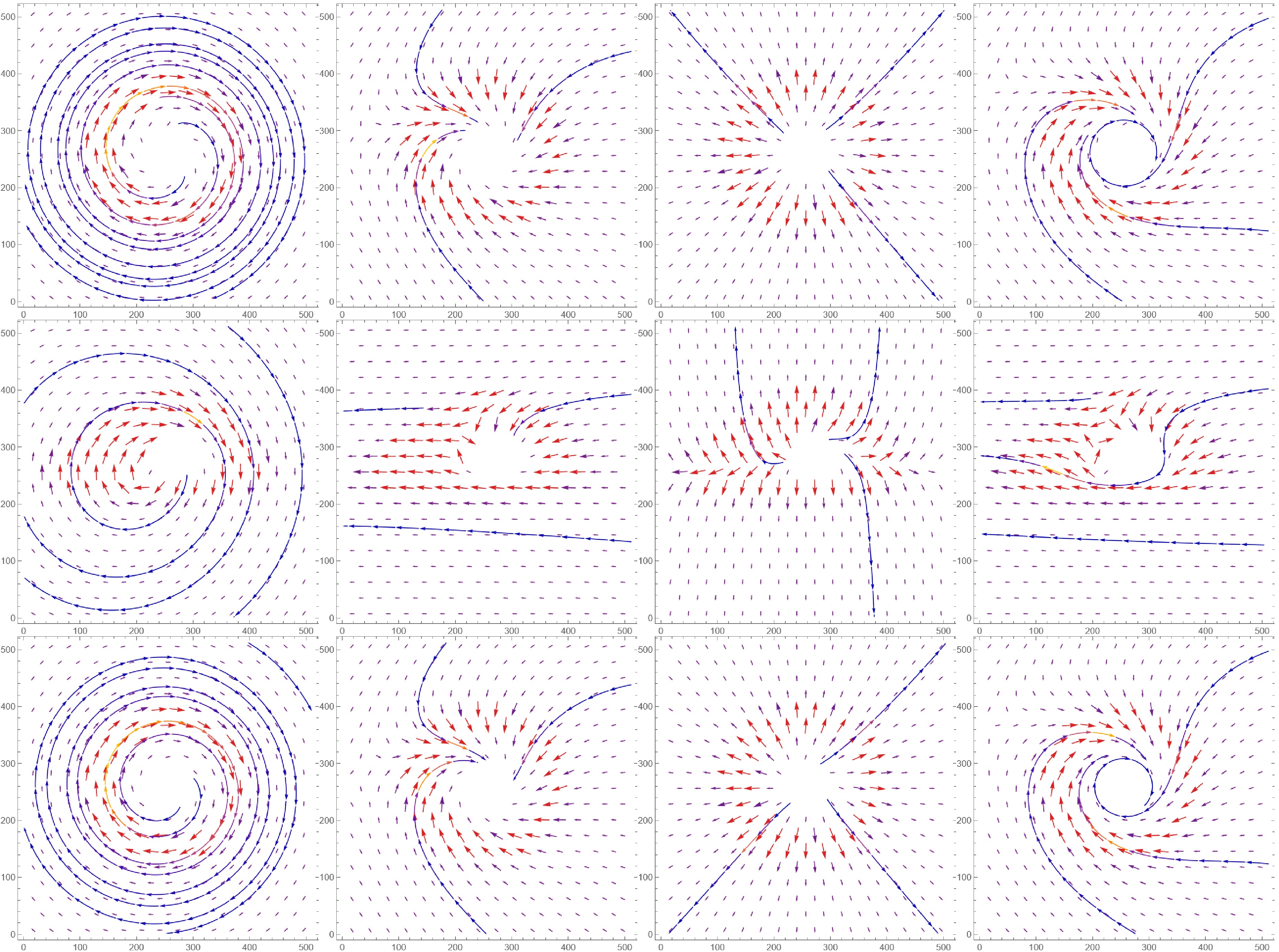
Figure 2. (color online) Polarization distribution and magnetic field configuration around a rotating Hayward BH, highlighting the effects of radial, θ-oriented, and ϕ-oriented magnetic fields, along with the configuration for M87*.
In the scenario where the magnetic field is oriented exclusively along the θ-direction (
$ B=(0,0,1,0) $ ), the polarization distribution exhibits a horizontal orientation on the western side. In contrast, in the northern and southern regions, the polarization vectors converge toward the center, causing the magnetic field lines to bend toward this focal point. As the observation inclination approaches$ \pi/2 $ , the magnetic field tilts toward a predominantly horizontal orientation.We next investigate the effects of a magnetic field oriented purely along the ϕ-direction, represented as
$ B=(0,0,0,1) $ . In this configuration, the polarization distribution radiates outward, with the magnetic field lines initially adopting a diagonal orientation at low inclination angles. As the inclination angle increases, the magnetic field lines progressively shift toward the center.The final column illustrates the magnetic field configuration corresponding to the polarization information of the M87* BH, given by
$ B=(0,0.87,0.5,0) $ . The polarization pattern evolves around the rotating Hayward BH, with the magnetic field lines adopting a smooth configuration. As the observation angle increases, the magnetic field lines exhibit a parallel alignment at large distances. However, near the BH, the field lines gradually tilt toward the southern direction.To further investigate the polarization properties around the rotating Hayward BH, we combine the BH image from the previous section with polarization information. The first three columns of Fig. 3 display polarization images corresponding to magnetic fields oriented along the θ- and ϕ-directions. For an observer inclination of
$ 17^\circ $ , a purely radial magnetic field produces a field distribution exhibiting a counterclockwise rotation, with polarization vectors concentrated near the photon ring. By contrast, a purely θ-directed magnetic field generates a polarization pattern that initially rotates counterclockwise before bending inward, whereas a purely ϕ-directed magnetic field results in a polarization configuration pointing outward from the center.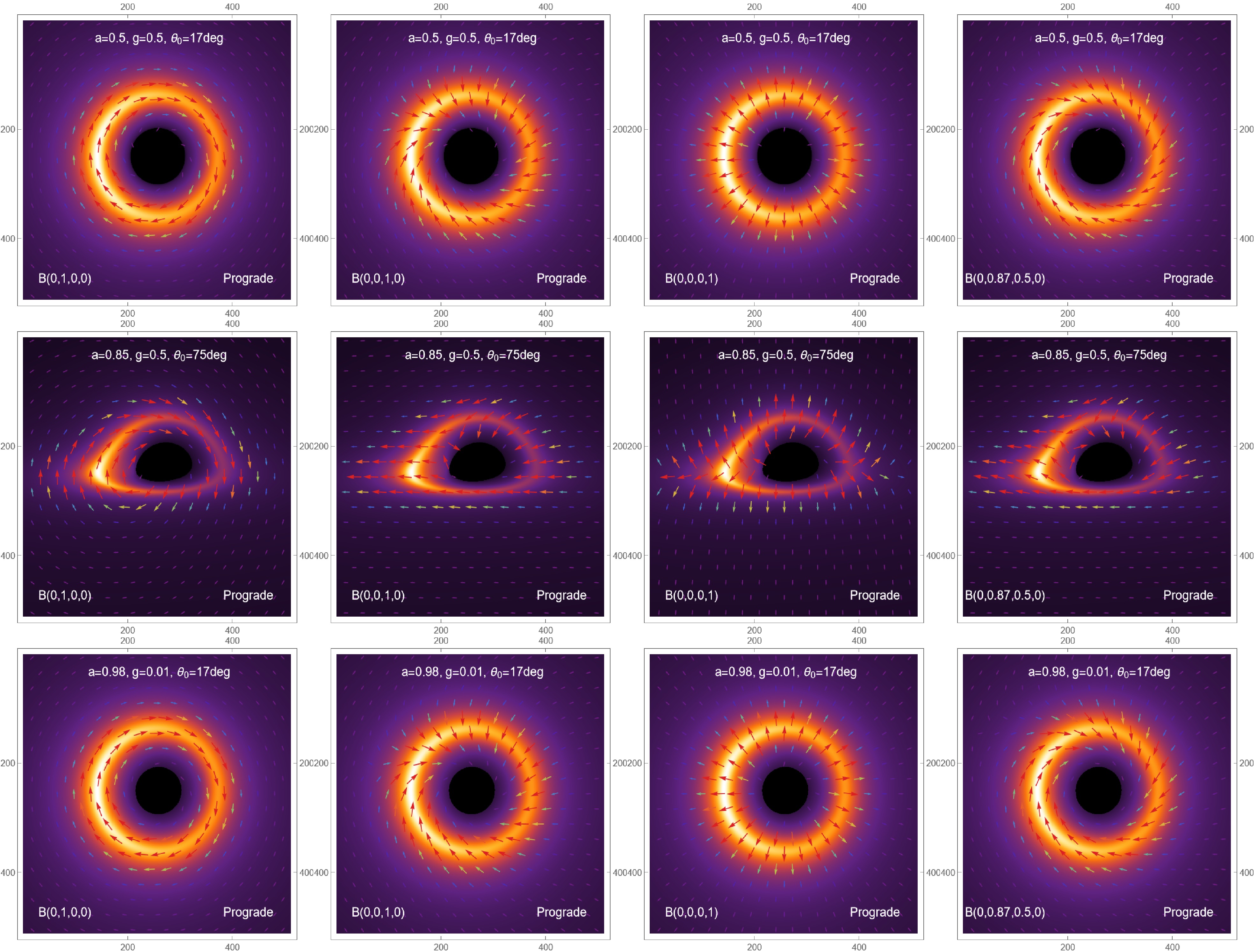
Figure 3. (color online) Polarization image of a rotating Hayward BH with a prograde accretion disk, illustrating the effects of radial, θ-oriented, and ϕ-oriented magnetic fields, along with the configuration for M87*.
As the observation angle increases, the polarization regions gradually flatten. With a radial magnetic field, the polarization retains a counterclockwise orientation. For a purely θ-directed field, the polarization in the inner region points toward the BH interior, whereas near the photon ring, it aligns horizontally. Conversely, a ϕ-oriented field produces an outward-pointing polarization distribution. Within the photon ring, the polarization becomes irregular and unstable, whereas outside the ring, it tends to align with the poles. Notably, variations in the spin and magnetic charge of the rotating Hayward BH scarcely affect the polarization features, suggesting that changes in these parameters have minimal observational impact. Aligning our magnetic field model with the predicted properties of M87* enhances its ability to forecast astrophysical BH characteristics. Expanding the polarization regions may reveal patterns similar to those observed in M87* and Sgr A*.
Figure 4 illustrates the polarization characteristics associated with a retrograde accretion disk. The results for radial, θ-oriented, and ϕ-oriented magnetic fields are presented, demonstrating consistency with the polarization patterns observed for prograde accretion disks.
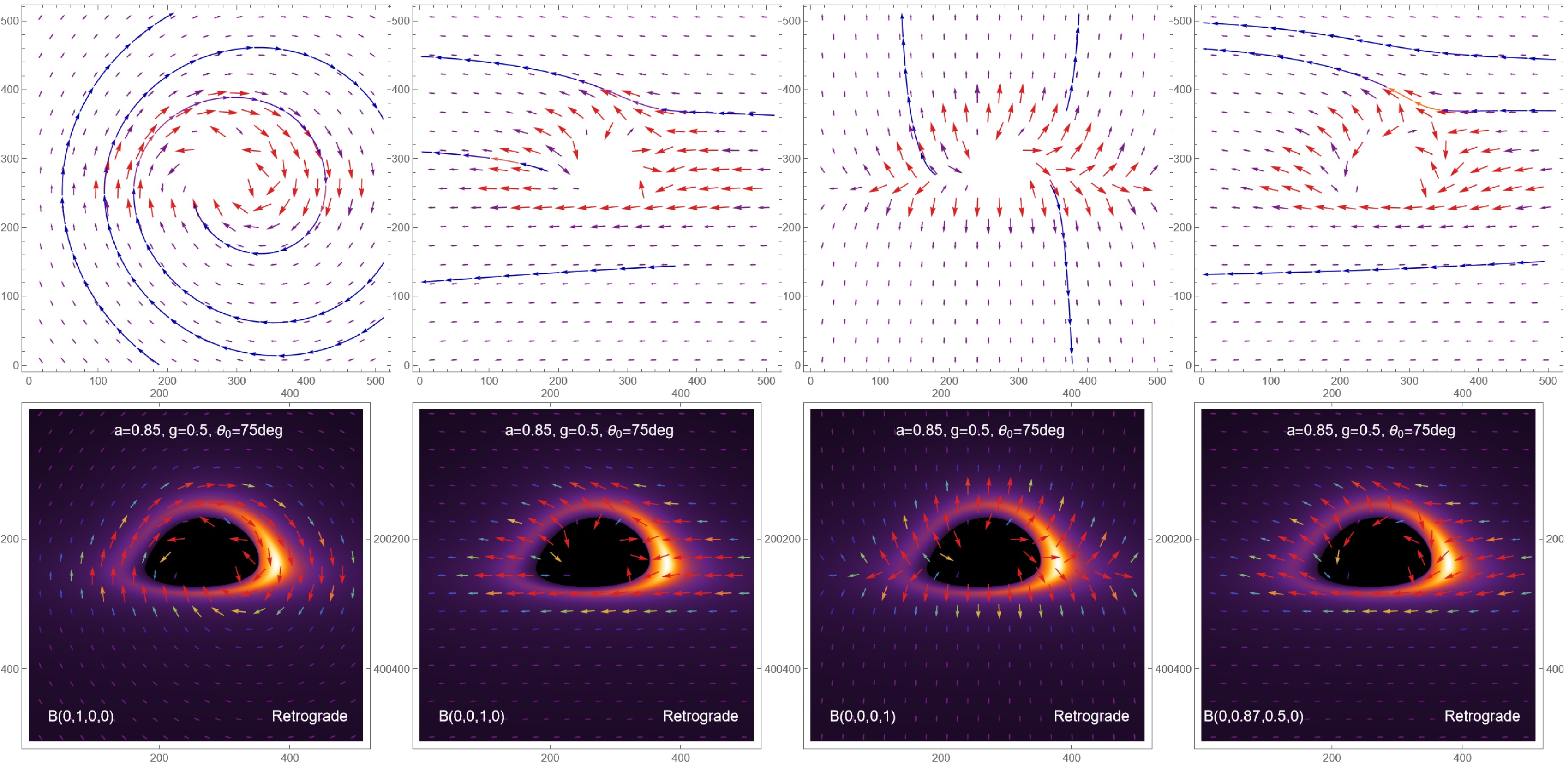
Figure 4. (color online) Polarization image of a rotating Hayward BH surrounded by a retrograde accretion disk, highlighting the effects of radial, θ-oriented, and ϕ-oriented magnetic fields, along with the magnetic field configuration for M87*.
The polarimetric image analysis of the rotating Hayward BH, presented in this section, offers significant insights into the underlying physics of BH environments, particularly in terms of the influence of magnetic field configurations on observed polarization patterns. Evaluation of the effects of radial, θ-oriented, and ϕ-oriented magnetic fields shows the mechanims by which the spacetime geometry and magnetic field structure around the Hayward BH impact the polarization of the emitted radiation. These findings highlight the utility of polarization as a powerful diagnostic tool for probing the properties of the accretion flow, magnetic fields, and event horizon of BH. The minimal impact of variations in spin and magnetic charge on the polarization suggests that such observations are robust across different parameter choices and ar thus especially valuable for testing BH models in future observational campaigns.
Figure 5 elucidates the polarization characteristics of a rotating Hayward BH surrounded by a prograde accretion disk under distinct magnetic field configurations. The polarization patterns, represented by EVPAs, reveal how spacetime geometry and magnetic field structure intertwine to imprint observable signatures. For a radial magnetic field
$ B \propto \dfrac{\partial}{\partial r} $ , the EVPAs exhibit a coherent counterclockwise spiral morphology, with the highest polarization concentration occurring near the photon ring. This alignment indicates the dominance of frame-dragging effects and radial orientation of the magnetic field in organizing the polarized emission. In contrast, a θ-oriented field ($ B \propto \partial_\theta $ ) produces a horizontal polarization pattern on the western side of the disk; within the northern and southern regions, the EVPAs converge radially toward the BH interior, reflecting the role of the poloidal field in bending the polarization vectors inward. A toroidal ϕ-oriented magnetic field$ \left( B \propto \dfrac{\partial}{\partial \phi} \right) $ generates an outward-radiating polarization distribution, signifying the role of azimuthal field lines in shaping the emission perpendicular to the orbital flow. Notably, the combined effects of the magnetic charge g and high spin a of the Hayward BH amplify the polarization degree within the photon-ring region. This enhancement manifests as pronounced Faraday rotation effects, which are attributable to the finite curvature of the nonsingular core modifying plasma interactions, and distinctive stripe-like interference patterns in the polarized intensity. These features serve as direct observational discriminators, distinguishing the Hayward BH from Kerr BHs. The final panel, calibrated to the inferred magnetic field geometry$ B= (0,0.87,0.5,0) $ of M87*, demonstrates a smoothly evolving polarization pattern, where field lines transition from parallel alignment at large distances to a gradual southward tilt near the event horizon, providing a testable model for future interferometric observations. The minimal variation in the polarization structure across changes in g and a suggests that these signatures are robust probes of accretion physics and spacetime geometry.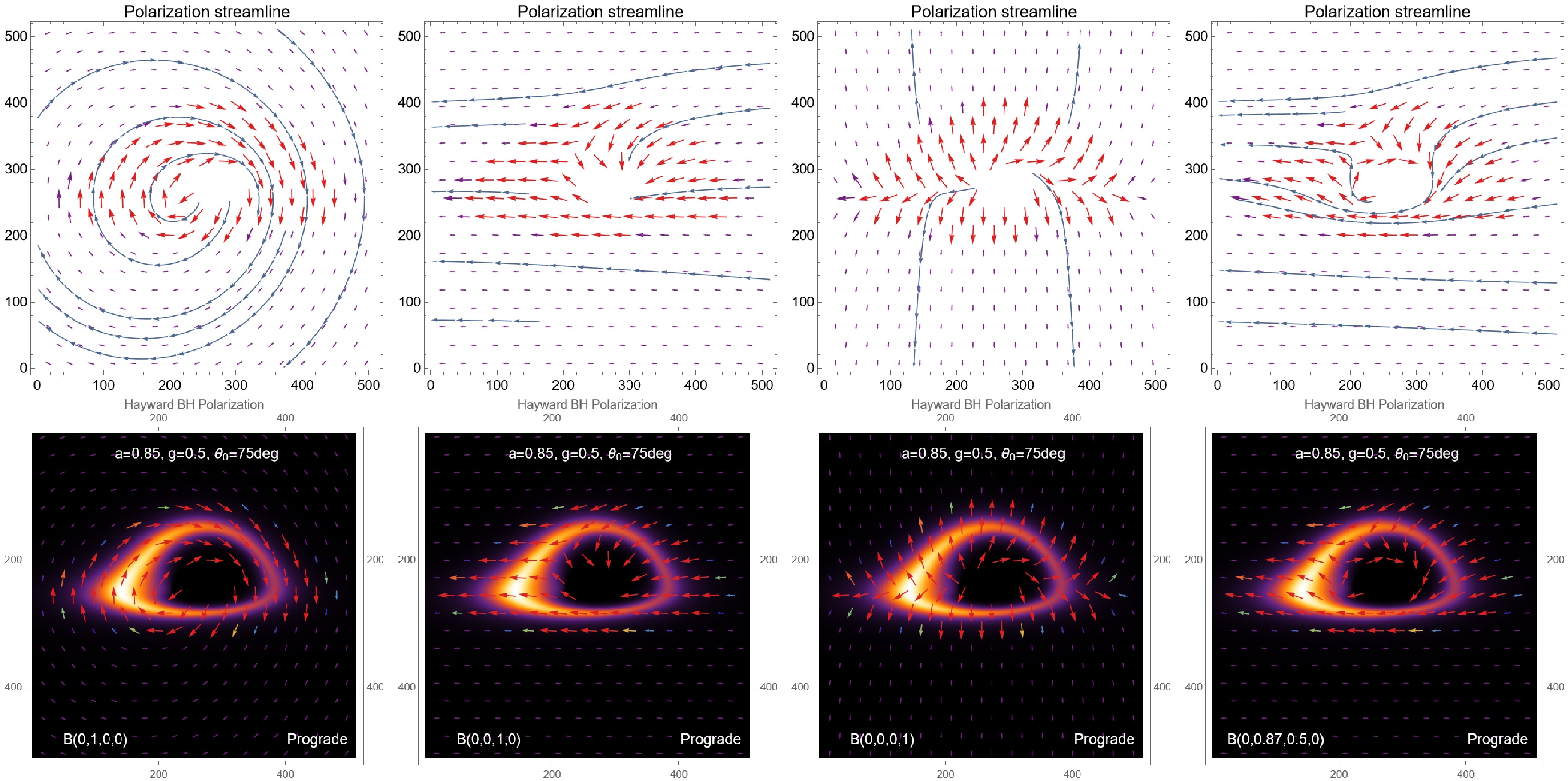
Figure 5. (color online) Polarization image of a rotating Hayward BH with a prograde accretion disk, illustrating the effects of radial, θ-oriented, and ϕ-oriented magnetic fields, along with the configuration for M87*.
Figure 6 illustrates the EVPA vector fields of the Hayward BH in the prograde case. When the viewing inclination is
$ \theta_0 = 17^\circ $ , the polarization field appears nearly axisymmetric, and the EVPAs extend approximately in a radial pattern. As the inclination increases to$ \theta_0 = 53^\circ $ , the EVPA distribution on the approaching side of the accretion disk shows noticeable rotations and shearing, which alter their local orientations. At a high inclination of$ \theta_0 = 75^\circ $ , these features become even more pronounced, generating strong asymmetry and forming spiral-like flow structures along the crescent. For a fixed viewing inclination, increasing the spin parameter amplifies the frame-dragging effect in the spacetime, shifting the polarization direction and reducing the polarization intensity toward smaller radii. Consequently, the azimuthal twisting of EVPAs becomes more distinct, with the vectors aligning more closely along the photon-ring ridge.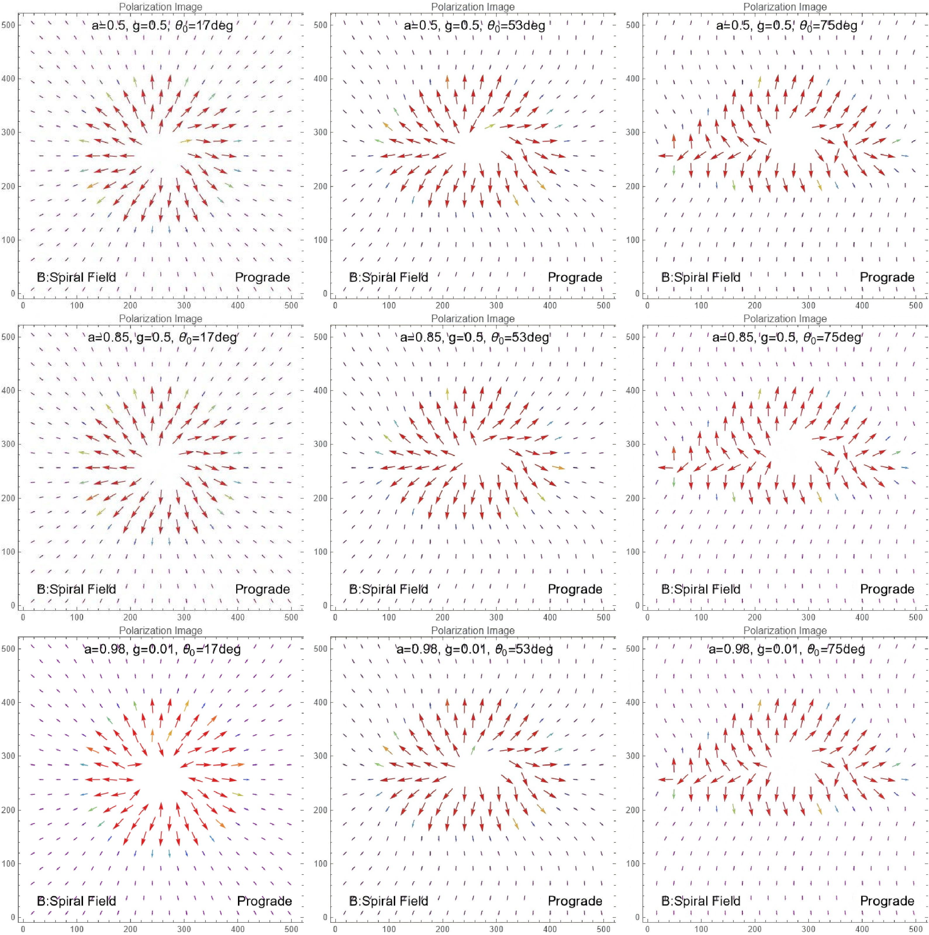
Figure 6. (color online) EVPA vector fields for prograde disks. From top to bottom:
$ a = 0.5, g = 0.5 $ ,$ a = 0.85, g = 0.5 $ , and$ a = 0.98, g = 0.01 $ . From left to right:$ 17^\circ $ ,$ 53^\circ $ ,$ 75^\circ $ . Red arrows show EVPA; color saturation tracks polarized intensity. The EVPAs reveal distinct polarization patterns induced by the B-spiral magnetic field configuration. High spin and magnetic charge amplify the polarization degreen in the photon-ring region, producing prominent Faraday rotation effects (attributable to finite curvature of the nonsingular core) and stripe-like interference patterns.Overall, a comparison of the three rows of images at the same inclination shows that at the extreme values of the spin and magnetic charge, the resulting polarization patterns differ only slightly from those of the other cases. This weak contrast is attributed to the partial cancellation between the reduced photon-ring size, caused by the changing magnetic charge, and the increased twisting, introduced by varying spin. From another perspective, this result demonstrates the strong correlation of the EVPA patterns with a, g, and
$ \theta_0 $ . However, evidently, variations in the viewing inclination produce the most significant changes in the EVPA morphology.Figure 7 presents the streamline characteristics of the EVPA. The streamlines pass through the shadow boundary almost radially. However, as the viewing inclination increases, they begin to twist rotationally on the approaching side. The separatrix curves encircle the shadow boundary and converge at the brightest region of the photon ring. The azimuthal winding number increases systematically with the BH spin parameter a, revealing the enhanced rotation induced by parallel transport in a more strongly dragged spacetime. Variations in the magnetic charge alter the turning behavior of the streamlines. With increasing magnetic charge, the spacing between adjacent streamlines decreases. This effect is particularly noticeable when comparing the second and third rows of the images, highlighting the significant influence of magnetic charge on the streamline structure.
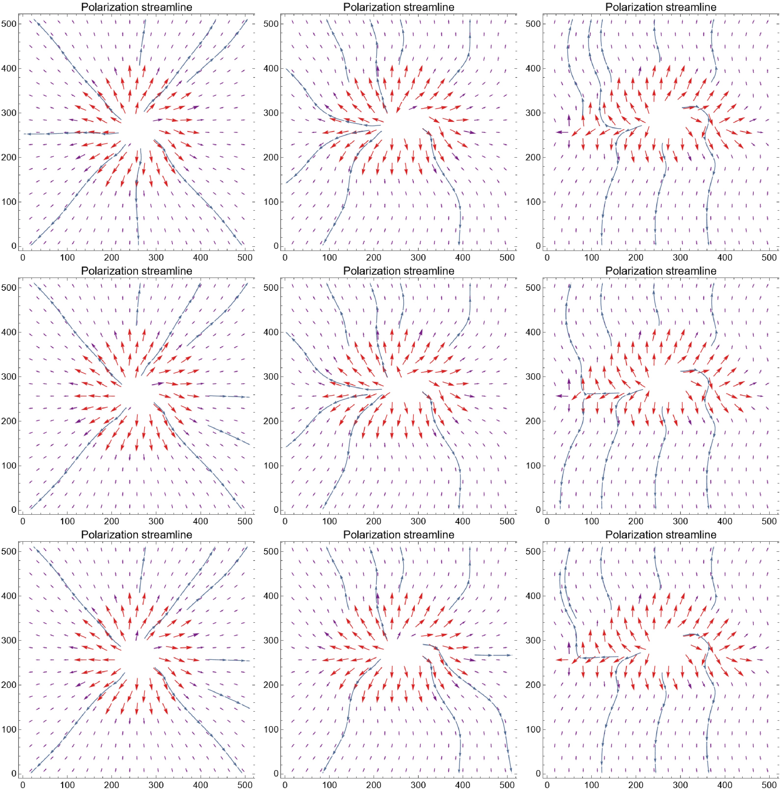
Figure 7. (color online) EVPA streamlines for prograde disks. Blue curves trace integral curves of the EVPA pseudo-vector, emphasizing global coherence and critical lines.
Figure 8 combines the radiation intensity with the EVPA arrow and streamline plots, enabling a direct connection between the polarization structure and underlying emission features. As the viewing inclination increases, the image gradually shifts from an almost symmetric ring to a distinctly crescent-shaped structure on the approaching side. The EVPA vectors follow the photon-ring ridge tangentially while showing controlled rotation across the ring thickness—a distinctive signature of general relativistic parallel transport. As the spin increases, the crescent region sharpens progressively, whereas a higher magnetic charge slightly contracts the photon ring and compresses the vector field. The arcsinhCγ stretch preserves faint halo-like emission without saturating the peak brightness, ensuring that the EVPA flips near the critical curve and that streamline coherence remains visible and comparable across all the panels.
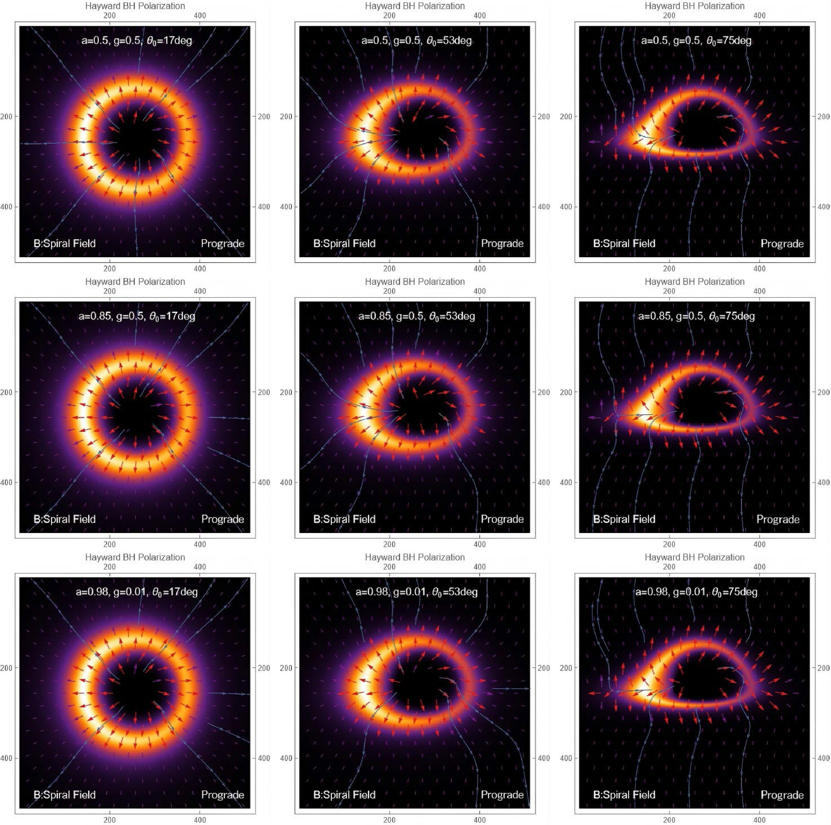
Figure 8. (color online) Polarization image of a rotating Hayward BH with a prograde accretion disk, illustrating the effects of radial, θ-oriented, and ϕ-oriented magnetic fields, along with the configuration for M87*.
Next, we analyze the polarization features of the accretion disk in the retrograde configuration. We adopt the same set of parameters as those used in the prograde case. However, because the retrograde disk has a larger ISCO radius and therefore a lower orbital velocity compared with the prograde case, its polarization signatures exhibit characteristic differences.
In Figure 9, the EVPA field at low viewing inclinations remains approximately radial in the retrograde case. However, its alignment with the photon-ring ridge is weaker than that in the prograde configuration. As the inclination increases, the EVPA rotation on the approaching side remains noticeable; however, its orientation becomes opposite to that in the prograde case. This reversal matches the opposite sign of the accumulated parallel-transport phase in a spacetime, where orbital motion counteracts frame dragging.
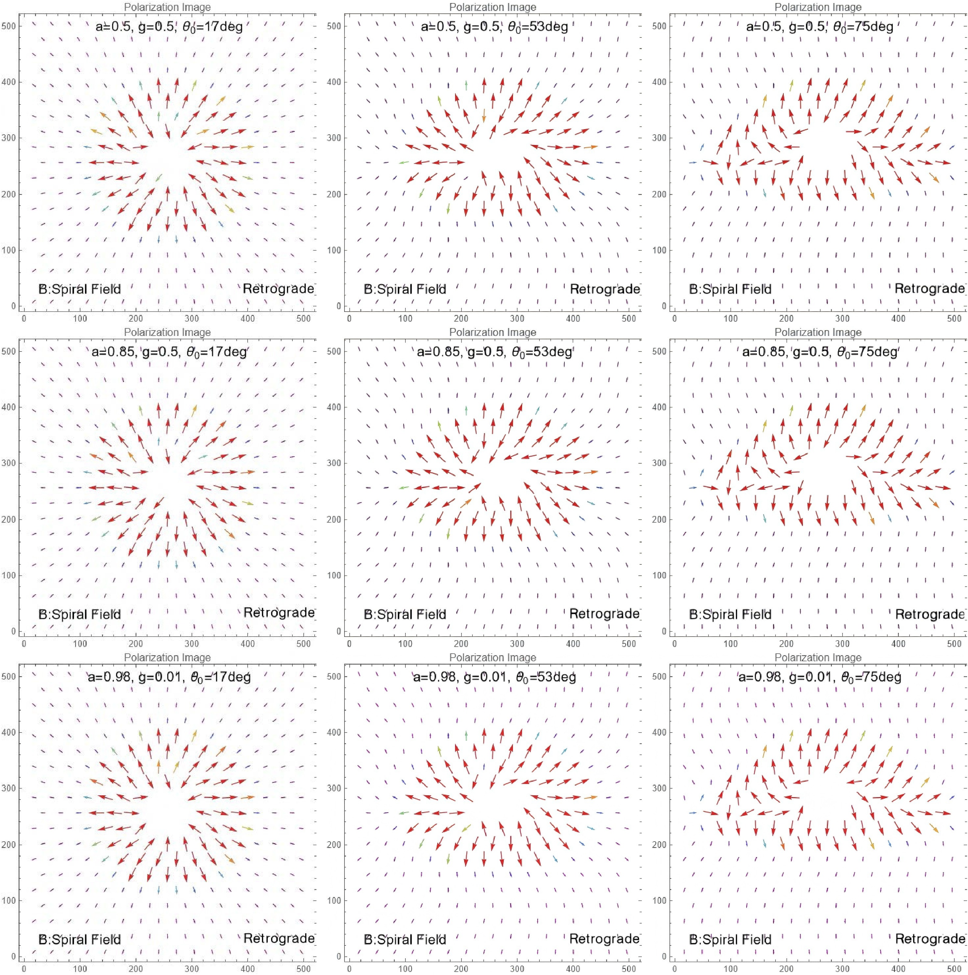
Figure 9. (color online) EVPA vector fields for retrograde disks. From top to bottom:
$ a = 0.5, g = 0.5 $ ,$ a = 0.85, g = 0.5 $ , and$ a = 0.98, g = 0.01 $ . From left to right:$ 17^\circ $ ,$ 53^\circ $ ,$ 75^\circ $ . Red arrows show EVPA; color saturation tracks polarized intensity. The EVPAs reveal distinct polarization patterns induced by the B-spiral magnetic field configuration. High spin and magnetic charge amplify the polarization degree in the photon-ring region, producing prominent Faraday rotation effects (attributable to finite curvature of the nonsingular core) and stripe-like interference patterns.For fixed
$ (g, \theta_0) $ , the azimuthal twisting continuously enhances as the spin increases from$ a=0.5 $ to$ a=0.85 $ . However, the net rotation amplitude at a given inclination is smaller than that in the prograde scenario, because the larger ISCO radius in the retrograde geometry weakens the frame dragging experienced by the emitting plasma. In the last row, where the spin reaches the extreme value$ a = 0.98 $ and the magnetic charge is minimal ($ g = 0.01 $ ), the EVPA field varies relatively slightly with increasing inclination compared to that in the the previous cases. This result suggests that the changes in the observed EVPA morphology are primarily driven by the viewing inclination.Figure 10 shows the EVPA streamline patterns for the retrograde accretion disk, exhibiting distinct reversal relative to the prograde case. In the retrograde configuration, the separatrix curves bend around the shadow boundary with the opposite rotational sense and tend to merge more easily at locations farther from the photon ring. The azimuthal winding number still increases with the spin parameter a; however, for the same
$ (a, \theta_0) $ , its magnitude is consistently lower than that in the corresponding prograde cases. This behavior reflects the weaker net frame dragging experienced by plasma on retrograde orbits.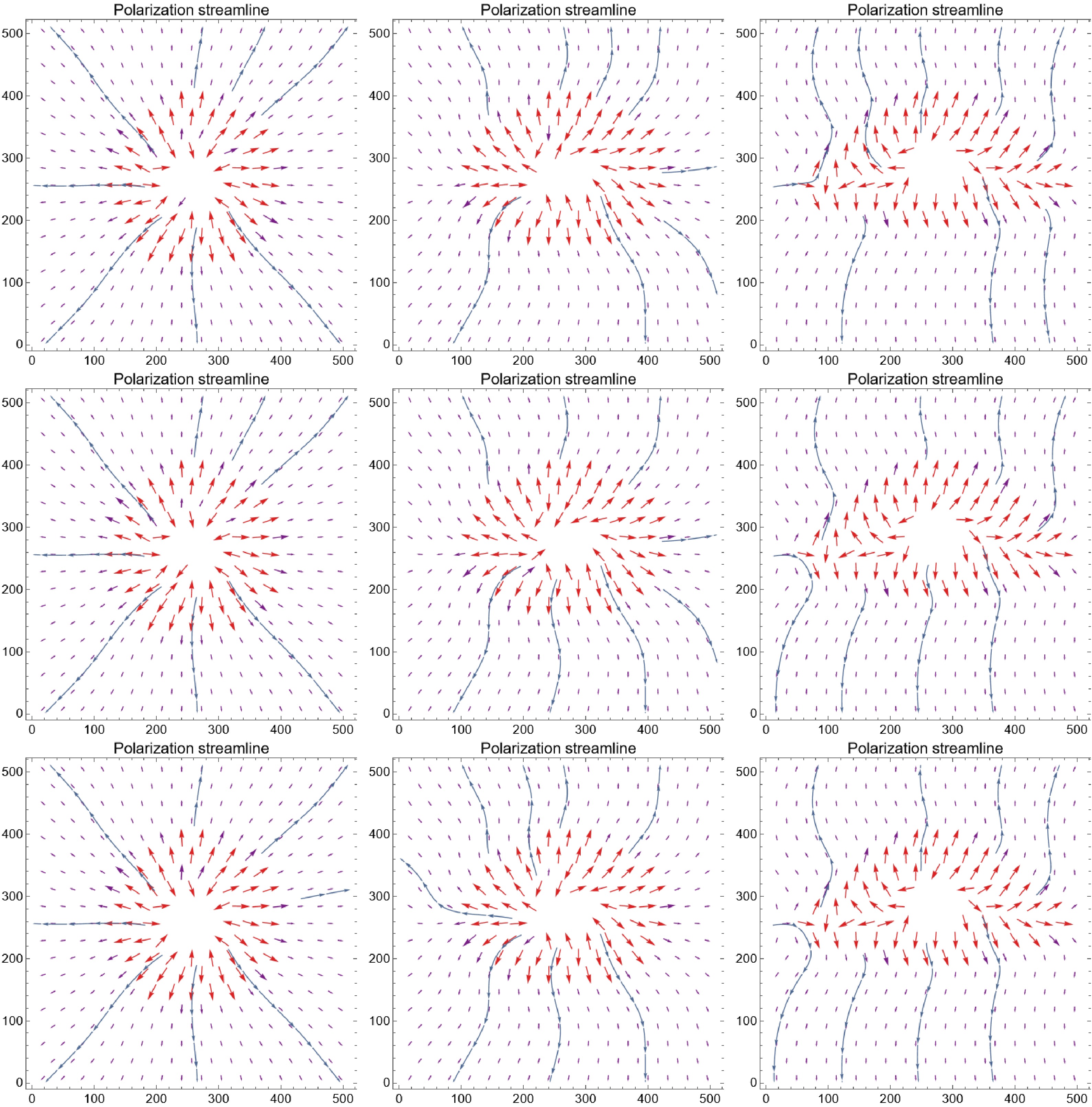
Figure 10. (color online) EVPA streamlines for retrograde disks. Blue curves trace integral curves of the EVPA pseudovector, emphasizing global coherence and critical lines.
Figure 11 presents the composite maps of total intensity and polarization in the retrograde configuration. Like the prograde case, a Doppler-boosted crescent emerges at high viewing inclinations; however, the crescent in the retrograde case is noticeably broader, and its peak less sharp, owing to the larger orbital radius and lower orbital velocity of the emitting material. The EVPA vectors exhibit an overall spiraling pattern with the opposite rotational sense. For a fixed spin parameter, magnetic charge, and viewing inclination, the azimuthal rotation rate of the EVPA along the photon-ring ridge is consistently lower than that in the prograde case. The arcsinh–γ stretch continues to preserve the faint outer halo, revealing that the EVPA flips, and the coherence of the streamlines occurs at radii farther from the shadow boundary compared to that in the corresponding prograde images.
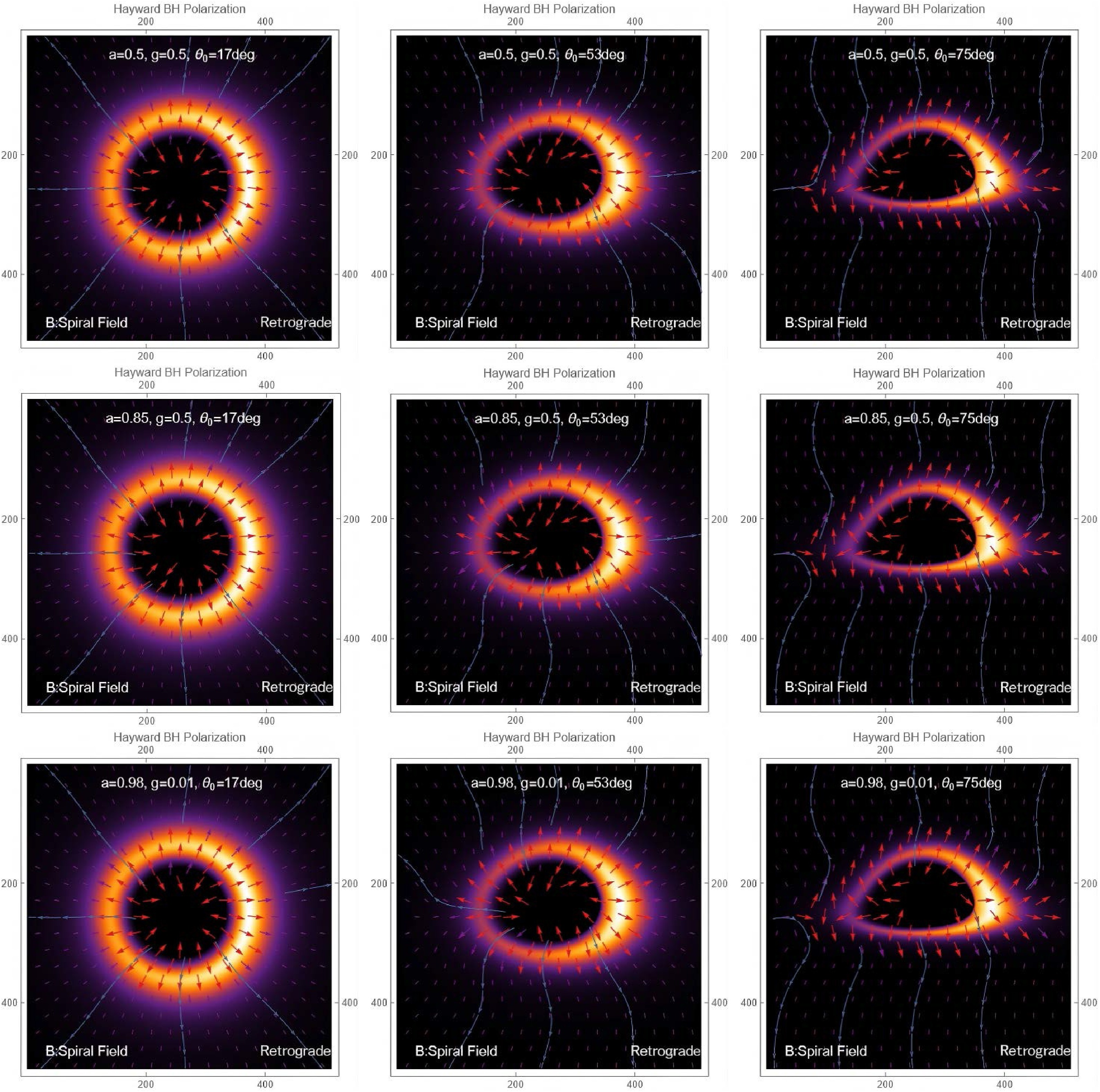
Figure 11. (color online) Polarization image of a rotating Hayward BH with a retrograde accretion disk, illustrating the effects of radial, θ-oriented, and ϕ-oriented magnetic fields, along with the configuration for M87*.
In summary, the combined use of (i) EVPA arrow maps, (ii) streamline topology, and (iii) total-intensity polarization composites provides a physically interpretable framework for distinguishing prograde from retrograde accretion flows in horizon-scale polarization measurements. In particular, the sign of the dynamical azimuthal EVPA rotation and degree of streamline winding along the bright ring serve as robust, colormap-independent features that can be directly compared with EHT observations.
In both the prograde and retrograde cases, increasing the spin parameter a universally amplifies the frame-dragging effect of the spacetime, thereby enhancing the polarization intensity and azimuthal twisting in the images. In contrast, the magnetic charge g exerts almost the opposite influence: larger values of g cause stronger attenuation of the polarization signal. Consequently, when a is near maximal, and g is close to minimal, the net variation in the EVPA morphology remains relatively modest. Nonetheless, across all the panels, the effect of viewing inclination is far more pronounced than that of either spin or magnetic charge.
These diagnostics directly connect the observed polarization patterns to the interplay among Doppler beaming, gravitational lensing, and spin-dependent parallel-transport phases in the Hayward spacetime. Thus, they provide a pathway for constraining
$ (a, g, \theta_0) $ using EHT class VLBI polarization data. -
In the preceding section, we presented the simulation results of a rotating Hayward BH surrounded by a thin accretion disk. Observational data from the EHT further demonstrate that polarimetric imaging of BHs, such as M87* and the supermassive BH at the center of the Milky Way, can reveal polarization information in their immediate vicinity [40–41, 43, 77]. Notably, strong linear polarization is observed from synchrotron emission at an observational wavelength of
$ 1.3 $ mm [40–41].The polarization state propagates through a magnetized plasma, undergoing Faraday rotation and transformation. Due to the complex interplay between emission and propagation effects, numerical radiative transfer calculations are crucial for accurately capturing the observed polarization of M87* and Sgr A*. In addition to the intensity component (Stokes
$ {\cal{I}} $ ), ray-tracing techniques can be employed to determine the observed linear polarization (Stokes$ {\cal{P}} = {\cal{Q}} + i {\cal{U}} $ ) and generate polarization images, as demonstrated in previous studies [78–79].Unlike in Euclidean space, the transport of a tensor along a manifold is path-dependent, requiring a consistent set of propagation rules to preserve “directional” invariance. Given a curve
$ {\cal{C}} $ on the manifold$ {\cal{M}} $ , with tangent vectors$ t^{\rm{u}} $ at each point, a tensor$ T^{\rho_1 \cdots \rho_k}_{\sigma _1 \cdots \sigma _l} $ remains covariant along$ {\cal{C}} $ if$ t^{ \mu} \nabla_{ \mu} T^{\rho_{1}\cdot\cdot\cdot\rho_{k}}_{\sigma _{1}\cdot\cdot\cdot\sigma _{l}} = 0. $
(48) If the tangent vector
$ t^{\mu} $ of$ {\cal{C}} $ is invariant along the curve, then the geodesic equation takes the form$ t^{\mu}\nabla_{\mu}t^{\nu}=0, $
(49) which translates to
$ \dfrac{{\rm{d}}^{2} x^{ \mu}}{{\rm{d}}\lambda^{2}} + \Gamma^{\mu}_{\nu \rho} \dfrac{{\rm{d}} x^{ \nu}}{{\rm{d}} \lambda} \dfrac{{\rm{d}} x^{ \rho}}{{\rm{d}} \lambda} = 0. $
(50) For a spacelike geodesic, the maximum arc length between two points a and b is given by
$ (\rm Arc Length)_{\rm max} = \int^{b}_{a} \sqrt{g_{\mu \nu} t^{\mu} t^{\nu}} {\rm{d}} \lambda. $
(51) For a timelike geodesic, the proper time between two points is given by
$ \Delta \tau = \int^{b}_{a} \sqrt{g_{\mu \nu} t^{\mu} t^{\nu}} {\rm{d}} \lambda. $
(52) We define the Lorentz-invariant Stokes vector as
$ {\bf{S}} = ({\cal{I}},{\cal{Q}},{\cal{U}},{\cal{V}}) $ . The radiative transfer equation for the Stokes vector in flat spacetime, along a ray parameterized by s, is given by [78]:$\begin{aligned}[b] \dfrac{\mathrm d}{\mathrm ds} \left( \begin{array}{c} I \\ Q \\ U \\ V \end{array} \right) =& \left( \begin{array}{c} j_{I} \\ j_{Q} \\ j_{U} \\ j_{V} \end{array} \right) \\& - \left( \begin{array}{cccc} \alpha_{I} & \alpha_{Q} & \alpha_{U} & \alpha_{V} \\ \alpha_{Q} & \alpha_{I} & \rho_{V} & -\rho_{U} \\ \alpha_{U} & -\rho_{V} & \alpha_{I} & \rho_{Q} \\ \alpha_{V} & \rho_{U} & -\rho_{Q} & \alpha_{I} \end{array} \right) \left( \begin{array}{c} I \\ Q \\ U \\ V \end{array} \right). \end{aligned} $
(53) Assuming
$ f^{ \mu} $ as the polarization vector orthogonal to the photon's momentum$ p_{\mu} $ , the polarization vector f satisfies the condition of parallel transport along the photon trajectory [80]:$ p^{ \mu} \nabla_{ \mu} f^{ \nu} = 0. $
(54) For a rotating Hayward BH, the photon trajectories, parameterized by
$ x^{\mu}(\tau) $ , have rescaled four-momentum components, which are given by$ p_{ \mu} {\rm{d}} x^{ \mu} = - {\rm{d}} t \pm_{\rm{r}} \dfrac{{\cal{V}}_{\rm{r}}(r)}{\Delta (r)} {\rm{d}} r \pm_{ \theta} \sqrt{{\cal{V}}_{ \theta}(\theta)} {\rm{d}} \theta + {\cal{L}} {\rm{d}} \phi. $
(55) The four-momentum
$ p_{\mu} $ of photons in the rotating Hayward BH is described by Eq. (55). By raising the exponent and expanding it in the asymptotic limit, we obtain the leading-order expansion:$ p^{ \mu} \partial_{ \mu} \approx \partial_{\rm{t}} \pm_{\rm{r}} \partial_{\rm{r}} \pm_{ \theta} \dfrac{\sqrt{{\cal{V}}_{\theta}( \theta)}}{r^{2}} \partial_{ \theta} + \dfrac{{\cal{L}}}{r^{2} \sin^{2}\theta} \partial_{ \phi}, $
(56) where the contributions from the subleading terms are suppressed in the inverse power expansion of r. Consequently, the light detected by a distant observer at a large radius
$ r \rightarrow \infty $ and an inclination angle$ \theta_{0} $ has the following four-momentum:$ p^{ \mu} \partial_{ \mu} = \partial_{\rm{t}} + \partial_{\rm{r}} + \dfrac{\beta}{r^{2}} \partial_{ \theta} - \dfrac{\alpha}{r^{2} \sin^{2}\theta} \partial_{\phi}. $
(57) At large radii, the four-momentum can be approximated as
$ p \cdot f \approx - f^{t} + f^{r} + \beta f^{\theta} - \alpha \sin \theta f^{\phi} $ . Consequently, the orthogonality condition, described in Eq. (55), implies that$ f^{\rm{r}} = f^{\rm{t}} - \beta f^{ \theta} + \alpha \sin f^{ \phi}. $
(58) To determine the polarization
$ f_{\rm{s}} $ of the source, we first define several key conditions:$ f_{\rm{s}} \cdot p_{\rm{s}} = 0,\; \; \; \; f_{\rm{s}} \cdot u_{\rm{s}} = 0,\; \; \; \; f_{\rm{s}} \cdot B_{\rm{s}} = 0. $
(59) The first condition stipulates that the polarization direction be orthogonal to the propagation direction of the light. The second condition ensures that the polarization vector remains purely spatial within the emission frame, as given by
$ f^{\rm{(t)}} = - f_{\rm{(t)}} = - f_{ \mu} {e}^{ \mu}_{\rm{(t)}} = - f_{\rm{s}} \cdot u_{\rm{s}}, $
(60) where t and s denote components in the local orthonormal frame
$ {e}^{ \mu}_{\rm{(t)}} $ of the source, with$ {e}^{ \mu}_{\rm{(t)}}=u^{ \mu}_{\rm{s}} $ , and μ represents spacetime components. This approach provides a fixed specification: under a transformation, the polarization vector shifts according to$ f_{\rm{s}} \rightarrow f_{\rm{s}} + c p_{\rm{s}} $ . This transformation preserves the first condition while modifying$ f_{\rm{s}} \cdot u_{\rm{s}} $ to$ c p_{\rm{s}} \cdot u_{s} $ . By setting$ c = - (f_{\rm{s}} \cdot u_{\rm{s}})/(f_{\rm{s}} \cdot u_{\rm{s}}) $ , we establish a gauge-invariant flow velocity that satisfies the second condition. The third condition enforces the perpendicularity of the polarization to the spacetime vector$ B_{\rm{s}} $ , which is a physical constraint described in Eq. (59). For simulating synchrotron radiation,$ B_{\rm{s}} $ can be considered as the local magnetic field.Notably, the condition
$ f_{\rm{s}} \cdot u_{\rm{s}} = 0 $ is crucial. We assume that the initial polarization vector$ f'_{\rm{s}} $ satisfies$ f'_{s} \cdot p_{s} = 0 $ , along with$ f'_{\rm{s}} \cdot u_{\rm{s}} = 0 $ and$ f'_{\rm{s}} \cdot B_{\rm{s}} = 0 $ . In this case, a specification offset$ f'_{\rm{s}} \rightarrow f_{\rm{s}} = f'_{\rm{s}} + c p_{\rm{s}} $ , where$ c = - (f'_{\rm{s}} \cdot B_{\rm{s}})/(P_{\rm{s}} \cdot B_{\rm{s}}) $ , results in a physically equivalent polarization vector that satisfies$ f_{\rm{s}} \cdot B_{\rm{s}} = 0 $ . Thus, through appropriate transformations, we can adjust the initial polarization to become perpendicular to the magnetic field, ensuring that the observed polarization remains invariant.According to Eq. (56), the four-momentum
$ p=p_{ \mu} {\rm{d}} x^{ \mu} $ of a photon in the spacetime of a rotating Hayward BH is expressed as$ p = {\cal{E}} \Big(- {\rm{d}} t \pm_{\rm{r}} \dfrac{{\cal{V}}_{\rm{r}}(r)}{\Delta (r)} {\rm{d}} r \pm_{ \theta} \sqrt{{\cal{V}}_{ \theta}(\theta)} {\rm{d}} \theta + {\cal{L}} {\rm{d}} \phi \Big). $
(61) This expression is characteristic of the spacetime geometry of a rotating Hayward BH. Furthermore, the Penrose–Walker constant κ, which is conserved along light rays, is defined in terms of the polarization vector
$ f^{ \mu} $ and four-momentum$ p^{ \mu} $ as$ \kappa = \kappa_{1} + {\rm i} \kappa_{2} = ({\cal{A}} - {\rm i} {\cal{B}}) (r - {\rm i} a \cos\theta), $
(62) $ {\cal{A}} = (p^{\rm{t}} f^{\rm{r}} - p^{\rm{r}} f^{\rm{t}}) + a \sin^{2}\theta (p^{\rm{r}} f^{ \phi} - p^{ \phi} f^{\rm{r}}), $
(63) $ {\cal{B}} = \Big((r^{2} + a^{2}) (p^{ \phi} f^{ \theta} - p^{ \theta} f^{ \phi}) - a (p^{\rm{t}} f^{ \theta} - p^{ \theta} f^{\rm{t}})\Big) \sin\theta. $
(64) Due to the Petrov type-D nature of the Hayward metric, the Penrose–Walker constant κ is conserved along null geodesics. This constant can be used algebraically to determine the linear polarization vector
$ f^{ \mu} $ of κ at the source, assuming parallel propagation. The existence of the Penrose–Walker constant κ, which originates from a conformal Killing tensor in the rotating Hayward BH spacetime, provides the foundation for the polarization modes. The trajectory of a photon reaching the observer at coordinates ($ \alpha,\beta $ ) can be traced back to the source, where the Penrose–Walker constant κ can be determined based on the photons initial polarization vector$ f^{ \mu} $ and four-momentum$ p^{ \mu} $ .The three conditions outlined in Eq. (60) constrain three of the four components of the source polarization vector
$ f_{\rm{s}}^{ \mu} $ , thereby establishing both its spatial and temporal directions. This, in turn, defines the observed EVPA. The remaining component determines the magnitude of the observed polarization; in our model, this magnitude is linked to the observed intensity$ I_{\rm{o}} $ at the observers location. As shown in Eq. (58), the large-radius expansion of Eq. (62) yields$ \kappa_{1} \approx (-r f^{ \theta}) \beta + (-r \sin \theta f^{ \phi}) \nu, $
(65) $ \kappa_2\approx(-rf^{\theta})\nu-(-r\sin\theta f^{\phi})\beta, $
(66) which can be inverted to obtain
$ - r f^{ \theta} = \dfrac{\beta \kappa_{1} + \nu \kappa_{2}}{\beta^{2} + \nu^{2}}, $
(67) $ - r \sin \theta f^{ \phi} = \dfrac{\nu \kappa_{1} - \beta \kappa_{2}}{\beta^{2} + \nu^{2}}. $
(68) At large radii, the polarization vector norm satisfies
$ f \cdot f \approx r^{2}[(f^{ \theta})^{2} + \sin^{2}\theta (f^{ \phi})^{2}] $ , which defines a basis for unit-normalized vectors such that$ f \cdot f =1 $ :$ \hat{\beta} = - \dfrac{1}{r} \partial_{ \theta}: (f^{ \theta}, f^{ \phi}) = \Big(-\dfrac{1}{r} , 0 \Big), $
(69) $ \hat{\alpha} = \dfrac{1}{r \sin \theta} \partial_{ \phi}: (f^{ \theta}, f^{ \phi}) = \Big( 0, \dfrac{1}{r \sin \theta} \Big), $
(70) where
$ \hat{\beta} $ and$ \hat{\alpha} $ are aligned with$ -\partial_{\theta} $ and$ \partial_{\phi} $ , respectively. Then, the polarization vector on the celestial sphere is given by$ f^{ \theta} \partial_{ \theta} + f^{ \phi} \partial_{ \phi} = (-r f^{ \theta}) \hat{\beta} + (r \sin \theta f^{ \phi})\hat{\alpha}, $
(71) with vector components on the observer's screen given by
$ (f_{ \alpha},f_{ \beta}) = \dfrac{1}{\beta^{2} + \nu^{2}} (\beta \kappa_{2} - \nu \kappa_{1}, \beta \kappa_{1} + \nu \kappa_{2}). $
(72) This vector
$ \vec{f} = f_{ \alpha} \hat{\alpha} + f_{ \beta} \hat{\beta} $ has a norm of$ \vec{f} \cdot \vec{f} = \dfrac{\kappa_{1}^{2} + \kappa_{2}^{2}}{\beta^{2} + \nu^{2}}. $
(73) The observed polarization, defined by the orientation of the electric field relative to the transverse momentum of the photon, is expressed as
$ \overrightarrow{{\cal{E}}} = ({\cal{E}}_{ \alpha},{\cal{E}}_{ \beta}) = \dfrac{(\beta \kappa_{2} - \nu \kappa_{1}, \beta \kappa_{1} +\nu \kappa_{2})}{\sqrt{(\kappa_{1}^{2} + \kappa_{2}^{2}) (\beta^{2} + \nu^{2})}}. $
(74) $ \nu = - (\alpha + a \sin\theta_{\rm{o}}). $
(75) Because the vector
$ \overrightarrow{{\cal{E}}} $ does not influence the EVPA,$ \chi = \arctan \left(- \dfrac{{\cal{E}}_{ \alpha}}{{\cal{E}}_{ \beta}} \right). $
(76) The Penrose–Walker constant in Eq. (62) can be interpreted as a scaling factor, which is excluded from the EVPA expression in Eq. (76). By solving Eq. (59), we obtain
$ b^{ \mu \nu} = B_{\rm{s}}^{ \mu} p_{\rm{s}}^{ \nu} - B_{\rm{s}}^{ \nu} p_{\rm{s}}^{ \mu} $ , which leads to$ f_{\rm{r}} = \dfrac{b^{ \theta \phi} - b^{{\rm{t}} \theta } \Omega}{b^{ \theta \phi} \iota + b^{{\rm{r}}\phi} \Omega} f_{\rm{t}}, $
(77) $ f_{ \theta} = \dfrac{b^{{\rm{r}}\phi} + b^{ {\rm{t}} \phi} \iota + b^{\rm{t r}} \Omega}{b^{ \theta \phi} \iota + b^{{\rm{r}}\phi} \Omega} f_{\rm{t}}, $
(78) $ f_{ \phi} = - \dfrac{b^{{\rm{r}}\theta} + b^{{\rm{t}} \theta } \iota}{b^{ \theta \phi} \iota + b^{{\rm{r}}\phi} \Omega} f_{\rm{t}}. $
(79) The EVPA encodes Stokes parameters
$ {\cal{Q}} $ and$ {\cal{U}} $ as the real and imaginary components, respectively, of the repolarization$ P_{\rm{o}} = {\cal{Q}} + i {\cal{U}} = m I_{\rm{o}}{\rm e}^{2{\rm i}\chi}, $
(80) where
$ I_{\rm{o}} $ represents the Stokes intensity, and$ 0 \leqslant m \leqslant 1 $ denotes the fractional degree of polarization. In a realistic model, m may vary across the image, because the polarization degree of photons generally depends on the angle between the emitted radiation and local magnetic field at the source. However, for simplicity, m can be treated as a constant to obtain a more tractable polarization image. This assumption is equivalent to assuming isotropic emission from the astrophysical source, allowing the emission profile$ I_{\rm{s}} $ to be treated as a scalar rather than a directional function. Under this approximation, the observed linear polarization amplitude can be written as$ P_{\rm{o}}=m I_{\rm{o}} $ , which preserves the total intensity profile$ I_{\rm{o}} $ while encoding the image structure through the EVPA orientation. The term “polarization scale” refers to the orientation of the polarization plane, i.e.,$ f_{\rm{o}} = m I_{\rm{o}} (- \sin\chi \partial_{\alpha} + \cos \chi \partial_{\beta}), $
(81) where χ is calculated based on the conservation of the Penrose–Walker constant κ, defined in Eq. (62), along with the polarization distribution of the light source specified for parallel propagation of the light rays. Notably, in the synchrotron emission models considered, half of the cases adopt the relation
$ m \propto \sin^{2}\xi $ , where ξ is the emission angle relative to the local magnetic field. However, the inclusion of this anisotropy only negligible affects the results. Thus, the polarization scale$ \big|f_{\rm{o}}\big|= \big|P_{\rm{o}}\big| \propto I_{\rm{o}} $ remains a reliable measure of the polarization magnitude.Figure 2 presents the polarization distribution and magnetic field configuration surrounding a rotating Hayward BH. The figure illustrates the polarization distribution patterns and magnetic field configurations for various magnetic field orientations. The first column shows a purely radial magnetic field, specified as
$ B=(0,1,0,0) $ . The resulting distribution exhibits an overall clockwise spiral pattern, with denser magnetic field lines observed at smaller observation angles ($ 0-\pi/2 $ ). As the observation angle increases, the magnetic field lines become more dispersed; however, they become dense again when the observation angle exceeds$ \pi/2 $ .
Figure 2. (color online) Polarization distribution and magnetic field configuration around a rotating Hayward BH, highlighting the effects of radial, θ-oriented, and ϕ-oriented magnetic fields, along with the configuration for M87*.
In the scenario where the magnetic field is oriented exclusively along the θ-direction (
$ B=(0,0,1,0) $ ), the polarization distribution exhibits a horizontal orientation on the western side. In contrast, in the northern and southern regions, the polarization vectors converge toward the center, causing the magnetic field lines to bend toward this focal point. As the observation inclination approaches$ \pi/2 $ , the magnetic field tilts toward a predominantly horizontal orientation.We next investigate the effects of a magnetic field oriented purely along the ϕ-direction, represented as
$ B=(0,0,0,1) $ . In this configuration, the polarization distribution radiates outward, with the magnetic field lines initially adopting a diagonal orientation at low inclination angles. As the inclination angle increases, the magnetic field lines progressively shift toward the center.The final column illustrates the magnetic field configuration corresponding to the polarization information of the M87* BH, given by
$ B=(0,0.87,0.5,0) $ . The polarization pattern evolves around the rotating Hayward BH, with the magnetic field lines adopting a smooth configuration. As the observation angle increases, the magnetic field lines exhibit a parallel alignment at large distances. However, near the BH, the field lines gradually tilt toward the southern direction.To further investigate the polarization properties around the rotating Hayward BH, we combine the BH image from the previous section with polarization information. The first three columns of Fig. 3 display polarization images corresponding to magnetic fields oriented along the θ- and ϕ-directions. For an observer inclination of
$ 17^\circ $ , a purely radial magnetic field produces a field distribution exhibiting a counterclockwise rotation, with polarization vectors concentrated near the photon ring. By contrast, a purely θ-directed magnetic field generates a polarization pattern that initially rotates counterclockwise before bending inward, whereas a purely ϕ-directed magnetic field results in a polarization configuration pointing outward from the center.
Figure 3. (color online) Polarization image of a rotating Hayward BH with a prograde accretion disk, illustrating the effects of radial, θ-oriented, and ϕ-oriented magnetic fields, along with the configuration for M87*.
As the observation angle increases, the polarization regions gradually flatten. With a radial magnetic field, the polarization retains a counterclockwise orientation. For a purely θ-directed field, the polarization in the inner region points toward the BH interior, whereas near the photon ring, it aligns horizontally. Conversely, a ϕ-oriented field produces an outward-pointing polarization distribution. Within the photon ring, the polarization becomes irregular and unstable, whereas outside the ring, it tends to align with the poles. Notably, variations in the spin and magnetic charge of the rotating Hayward BH scarcely affect the polarization features, suggesting that changes in these parameters have minimal observational impact. Aligning our magnetic field model with the predicted properties of M87* enhances its ability to forecast astrophysical BH characteristics. Expanding the polarization regions may reveal patterns similar to those observed in M87* and Sgr A*.
Figure 4 illustrates the polarization characteristics associated with a retrograde accretion disk. The results for radial, θ-oriented, and ϕ-oriented magnetic fields are presented, demonstrating consistency with the polarization patterns observed for prograde accretion disks.
Figure 4. (color online) Polarization image of a rotating Hayward BH surrounded by a retrograde accretion disk, highlighting the effects of radial, θ-oriented, and ϕ-oriented magnetic fields, along with the magnetic field configuration for M87*.
The polarimetric image analysis of the rotating Hayward BH, presented in this section, offers significant insights into the underlying physics of BH environments, particularly in terms of the influence of magnetic field configurations on observed polarization patterns. Evaluation of the effects of radial, θ-oriented, and ϕ-oriented magnetic fields shows the mechanims by which the spacetime geometry and magnetic field structure around the Hayward BH impact the polarization of the emitted radiation. These findings highlight the utility of polarization as a powerful diagnostic tool for probing the properties of the accretion flow, magnetic fields, and event horizon of BH. The minimal impact of variations in spin and magnetic charge on the polarization suggests that such observations are robust across different parameter choices and ar thus especially valuable for testing BH models in future observational campaigns.
Figure 5 elucidates the polarization characteristics of a rotating Hayward BH surrounded by a prograde accretion disk under distinct magnetic field configurations. The polarization patterns, represented by EVPAs, reveal how spacetime geometry and magnetic field structure intertwine to imprint observable signatures. For a radial magnetic field
$ B \propto \dfrac{\partial}{\partial r} $ , the EVPAs exhibit a coherent counterclockwise spiral morphology, with the highest polarization concentration occurring near the photon ring. This alignment indicates the dominance of frame-dragging effects and radial orientation of the magnetic field in organizing the polarized emission. In contrast, a θ-oriented field ($ B \propto \partial_\theta $ ) produces a horizontal polarization pattern on the western side of the disk; within the northern and southern regions, the EVPAs converge radially toward the BH interior, reflecting the role of the poloidal field in bending the polarization vectors inward. A toroidal ϕ-oriented magnetic field$ \left( B \propto \dfrac{\partial}{\partial \phi} \right) $ generates an outward-radiating polarization distribution, signifying the role of azimuthal field lines in shaping the emission perpendicular to the orbital flow. Notably, the combined effects of the magnetic charge g and high spin a of the Hayward BH amplify the polarization degree within the photon-ring region. This enhancement manifests as pronounced Faraday rotation effects, which are attributable to the finite curvature of the nonsingular core modifying plasma interactions, and distinctive stripe-like interference patterns in the polarized intensity. These features serve as direct observational discriminators, distinguishing the Hayward BH from Kerr BHs. The final panel, calibrated to the inferred magnetic field geometry$ B= (0,0.87,0.5,0) $ of M87*, demonstrates a smoothly evolving polarization pattern, where field lines transition from parallel alignment at large distances to a gradual southward tilt near the event horizon, providing a testable model for future interferometric observations. The minimal variation in the polarization structure across changes in g and a suggests that these signatures are robust probes of accretion physics and spacetime geometry.
Figure 5. (color online) Polarization image of a rotating Hayward BH with a prograde accretion disk, illustrating the effects of radial, θ-oriented, and ϕ-oriented magnetic fields, along with the configuration for M87*.
Figure 6 illustrates the EVPA vector fields of the Hayward BH in the prograde case. When the viewing inclination is
$ \theta_0 = 17^\circ $ , the polarization field appears nearly axisymmetric, and the EVPAs extend approximately in a radial pattern. As the inclination increases to$ \theta_0 = 53^\circ $ , the EVPA distribution on the approaching side of the accretion disk shows noticeable rotations and shearing, which alter their local orientations. At a high inclination of$ \theta_0 = 75^\circ $ , these features become even more pronounced, generating strong asymmetry and forming spiral-like flow structures along the crescent. For a fixed viewing inclination, increasing the spin parameter amplifies the frame-dragging effect in the spacetime, shifting the polarization direction and reducing the polarization intensity toward smaller radii. Consequently, the azimuthal twisting of EVPAs becomes more distinct, with the vectors aligning more closely along the photon-ring ridge.
Figure 6. (color online) EVPA vector fields for prograde disks. From top to bottom:
$ a = 0.5, g = 0.5 $ ,$ a = 0.85, g = 0.5 $ , and$ a = 0.98, g = 0.01 $ . From left to right:$ 17^\circ $ ,$ 53^\circ $ ,$ 75^\circ $ . Red arrows show EVPA; color saturation tracks polarized intensity. The EVPAs reveal distinct polarization patterns induced by the B-spiral magnetic field configuration. High spin and magnetic charge amplify the polarization degreen in the photon-ring region, producing prominent Faraday rotation effects (attributable to finite curvature of the nonsingular core) and stripe-like interference patterns.Overall, a comparison of the three rows of images at the same inclination shows that at the extreme values of the spin and magnetic charge, the resulting polarization patterns differ only slightly from those of the other cases. This weak contrast is attributed to the partial cancellation between the reduced photon-ring size, caused by the changing magnetic charge, and the increased twisting, introduced by varying spin. From another perspective, this result demonstrates the strong correlation of the EVPA patterns with a, g, and
$ \theta_0 $ . However, evidently, variations in the viewing inclination produce the most significant changes in the EVPA morphology.Figure 7 presents the streamline characteristics of the EVPA. The streamlines pass through the shadow boundary almost radially. However, as the viewing inclination increases, they begin to twist rotationally on the approaching side. The separatrix curves encircle the shadow boundary and converge at the brightest region of the photon ring. The azimuthal winding number increases systematically with the BH spin parameter a, revealing the enhanced rotation induced by parallel transport in a more strongly dragged spacetime. Variations in the magnetic charge alter the turning behavior of the streamlines. With increasing magnetic charge, the spacing between adjacent streamlines decreases. This effect is particularly noticeable when comparing the second and third rows of the images, highlighting the significant influence of magnetic charge on the streamline structure.
Figure 7. (color online) EVPA streamlines for prograde disks. Blue curves trace integral curves of the EVPA pseudo-vector, emphasizing global coherence and critical lines.
Figure 8 combines the radiation intensity with the EVPA arrow and streamline plots, enabling a direct connection between the polarization structure and underlying emission features. As the viewing inclination increases, the image gradually shifts from an almost symmetric ring to a distinctly crescent-shaped structure on the approaching side. The EVPA vectors follow the photon-ring ridge tangentially while showing controlled rotation across the ring thickness—a distinctive signature of general relativistic parallel transport. As the spin increases, the crescent region sharpens progressively, whereas a higher magnetic charge slightly contracts the photon ring and compresses the vector field. The arcsinhCγ stretch preserves faint halo-like emission without saturating the peak brightness, ensuring that the EVPA flips near the critical curve and that streamline coherence remains visible and comparable across all the panels.
Figure 8. (color online) Polarization image of a rotating Hayward BH with a prograde accretion disk, illustrating the effects of radial, θ-oriented, and ϕ-oriented magnetic fields, along with the configuration for M87*.
Next, we analyze the polarization features of the accretion disk in the retrograde configuration. We adopt the same set of parameters as those used in the prograde case. However, because the retrograde disk has a larger ISCO radius and therefore a lower orbital velocity compared with the prograde case, its polarization signatures exhibit characteristic differences.
In Figure 9, the EVPA field at low viewing inclinations remains approximately radial in the retrograde case. However, its alignment with the photon-ring ridge is weaker than that in the prograde configuration. As the inclination increases, the EVPA rotation on the approaching side remains noticeable; however, its orientation becomes opposite to that in the prograde case. This reversal matches the opposite sign of the accumulated parallel-transport phase in a spacetime, where orbital motion counteracts frame dragging.
Figure 9. (color online) EVPA vector fields for retrograde disks. From top to bottom:
$ a = 0.5, g = 0.5 $ ,$ a = 0.85, g = 0.5 $ , and$ a = 0.98, g = 0.01 $ . From left to right:$ 17^\circ $ ,$ 53^\circ $ ,$ 75^\circ $ . Red arrows show EVPA; color saturation tracks polarized intensity. The EVPAs reveal distinct polarization patterns induced by the B-spiral magnetic field configuration. High spin and magnetic charge amplify the polarization degree in the photon-ring region, producing prominent Faraday rotation effects (attributable to finite curvature of the nonsingular core) and stripe-like interference patterns.For fixed
$ (g, \theta_0) $ , the azimuthal twisting continuously enhances as the spin increases from$ a=0.5 $ to$ a=0.85 $ . However, the net rotation amplitude at a given inclination is smaller than that in the prograde scenario, because the larger ISCO radius in the retrograde geometry weakens the frame dragging experienced by the emitting plasma. In the last row, where the spin reaches the extreme value$ a = 0.98 $ and the magnetic charge is minimal ($ g = 0.01 $ ), the EVPA field varies relatively slightly with increasing inclination compared to that in the the previous cases. This result suggests that the changes in the observed EVPA morphology are primarily driven by the viewing inclination.Figure 10 shows the EVPA streamline patterns for the retrograde accretion disk, exhibiting distinct reversal relative to the prograde case. In the retrograde configuration, the separatrix curves bend around the shadow boundary with the opposite rotational sense and tend to merge more easily at locations farther from the photon ring. The azimuthal winding number still increases with the spin parameter a; however, for the same
$ (a, \theta_0) $ , its magnitude is consistently lower than that in the corresponding prograde cases. This behavior reflects the weaker net frame dragging experienced by plasma on retrograde orbits.
Figure 10. (color online) EVPA streamlines for retrograde disks. Blue curves trace integral curves of the EVPA pseudovector, emphasizing global coherence and critical lines.
Figure 11 presents the composite maps of total intensity and polarization in the retrograde configuration. Like the prograde case, a Doppler-boosted crescent emerges at high viewing inclinations; however, the crescent in the retrograde case is noticeably broader, and its peak less sharp, owing to the larger orbital radius and lower orbital velocity of the emitting material. The EVPA vectors exhibit an overall spiraling pattern with the opposite rotational sense. For a fixed spin parameter, magnetic charge, and viewing inclination, the azimuthal rotation rate of the EVPA along the photon-ring ridge is consistently lower than that in the prograde case. The arcsinh–γ stretch continues to preserve the faint outer halo, revealing that the EVPA flips, and the coherence of the streamlines occurs at radii farther from the shadow boundary compared to that in the corresponding prograde images.
Figure 11. (color online) Polarization image of a rotating Hayward BH with a retrograde accretion disk, illustrating the effects of radial, θ-oriented, and ϕ-oriented magnetic fields, along with the configuration for M87*.
In summary, the combined use of (i) EVPA arrow maps, (ii) streamline topology, and (iii) total-intensity polarization composites provides a physically interpretable framework for distinguishing prograde from retrograde accretion flows in horizon-scale polarization measurements. In particular, the sign of the dynamical azimuthal EVPA rotation and degree of streamline winding along the bright ring serve as robust, colormap-independent features that can be directly compared with EHT observations.
In both the prograde and retrograde cases, increasing the spin parameter a universally amplifies the frame-dragging effect of the spacetime, thereby enhancing the polarization intensity and azimuthal twisting in the images. In contrast, the magnetic charge g exerts almost the opposite influence: larger values of g cause stronger attenuation of the polarization signal. Consequently, when a is near maximal, and g is close to minimal, the net variation in the EVPA morphology remains relatively modest. Nonetheless, across all the panels, the effect of viewing inclination is far more pronounced than that of either spin or magnetic charge.
These diagnostics directly connect the observed polarization patterns to the interplay among Doppler beaming, gravitational lensing, and spin-dependent parallel-transport phases in the Hayward spacetime. Thus, they provide a pathway for constraining
$ (a, g, \theta_0) $ using EHT class VLBI polarization data. -
In this study, we propose a comprehensive and self-consistent framework for modeling the polarized appearance of Hayward BHs surrounded by geometrically thin, optically tenuous accretion flows. This framework integrates several key components: Hamiltonian-based ray tracing in the Hayward geometry, covariant construction and faithful parallel transport of the polarization four-vector, and a polarized emissivity prescription that explicitly accounts for the magnetic charge while retaining angular, spectral, and spatial dependence. In contrast to earlier studies, the present work advances the field in two noteworthy ways. First, we implement full general relativistic polarization transport in a rotating, magnetically charged, nonsingular spacetime. Second, we introduce a highly flexible polarized emission model that unifies anisotropic angular features, frequency-dependent behavior, and intrinsic brightness asymmetries. The generalized emissivity framework employs a spatial kernel with a tunable outer-tail index, coupled with a Planck-inspired spectral term, providing sufficient flexibility to represent disks, jets, and coronal structures. Representative magnetic-field configurations are constructed in the ZAMO frame and then projected onto the image plane, allowing precise control over local polarization degrees and EVPA orientations for optically thin synchrotron emission.
Magnetic charge in the Hayward metric leaves persistent and monotonic polarization imprints on the resulting images, largely independent of variations in the emissivity model. Increasing the magnetic charge g systematically modifies both the apparent photon-ring diameter and azimuthal span of coherent EVPAs, with the strongest effects occurring at high inclination angles. These behaviors arise from the combined influence of magnetic charge on photon geodesics and the accumulated parallel-transport phase along strongly lensed trajectories. For a fixed parameter set
$ (a, g, \theta_0) $ , prograde accretion flows show more pronounced EVPA rotation and tightly wound polarization streamlines near the photon ring. By contrast, retrograde flows produce broader, smoother crescent structures with opposite EVPA handedness. Enhancing the spin parameter a consistently amplifies the spacetimes frame-dragging effect, thereby enhancing the observed polarization amplitude and azimuthal twisting. In contrast, increasing g attenuates the overall polarization strength and diminishes the azimuthal structure.The adoption of a frequency-dependent factor of the form
$ \nu^3 \bigl({\rm e}^{\nu/T(r)} - 1\bigr)^{-1} $ further compresses and attenuates the high-frequency emission profile, enabling multiband polarimetric analysis. The$ {{\rm{arcsinh}}} $ –γ tone-mapping procedure preserves a wide dynamic range while maintaining EVPA legibility, facilitating direct comparisons with EHT-class polarimetric datasets. From a theoretical perspective, employing the Hamiltonian geodesic formulation together with the corresponding connection for polarization transport ensures strict consistency between photon trajectories and the evolution of Stokes parameters. This unified description resolves inconsistencies present in previous modeling efforts and clarifies the mechanism by which magnetic charge simultaneously affects the geodesic structure and polarization transport.Several simplifying assumptions still apply. In this study, we employ steady, optically thin emissivities and parametrized magnetic fields, without accounting for the temporal variability inherent to GRMHD simulations or the Faraday rotation/conversion expected from detailed plasma microphysics. Although the phenomenological frequency dependence captures the main trends, the precise spectral shape remains highly sensitive to the underlying electron distribution and thermodynamic state. Moreover, despite the visualization benefits of the
$ {{\rm{arcsinh}}}\gamma $ mapping, rigorous parameter estimation ultimately requires forward modeling in the visibility domain.In conclusion, polarization offers a powerful and independent avenue for disentangling the degeneracy among spin, magnetic charge, and viewing inclination in Hayward spacetimes. The suite of polarization diagnostics identified in this study—including EVPA handedness and rotation amplitude, streamline geometries, g-driven photon-ring scalings, and percent-level circular polarization—constitutes a practical and observation-ready toolkit for forthcoming horizon-scale VLBI polarimetry of BHs.
-
In this study, we propose a comprehensive and self-consistent framework for modeling the polarized appearance of Hayward BHs surrounded by geometrically thin, optically tenuous accretion flows. This framework integrates several key components: Hamiltonian-based ray tracing in the Hayward geometry, covariant construction and faithful parallel transport of the polarization four-vector, and a polarized emissivity prescription that explicitly accounts for the magnetic charge while retaining angular, spectral, and spatial dependence. In contrast to earlier studies, the present work advances the field in two noteworthy ways. First, we implement full general relativistic polarization transport in a rotating, magnetically charged, nonsingular spacetime. Second, we introduce a highly flexible polarized emission model that unifies anisotropic angular features, frequency-dependent behavior, and intrinsic brightness asymmetries. The generalized emissivity framework employs a spatial kernel with a tunable outer-tail index, coupled with a Planck-inspired spectral term, providing sufficient flexibility to represent disks, jets, and coronal structures. Representative magnetic-field configurations are constructed in the ZAMO frame and then projected onto the image plane, allowing precise control over local polarization degrees and EVPA orientations for optically thin synchrotron emission.
Magnetic charge in the Hayward metric leaves persistent and monotonic polarization imprints on the resulting images, largely independent of variations in the emissivity model. Increasing the magnetic charge g systematically modifies both the apparent photon-ring diameter and azimuthal span of coherent EVPAs, with the strongest effects occurring at high inclination angles. These behaviors arise from the combined influence of magnetic charge on photon geodesics and the accumulated parallel-transport phase along strongly lensed trajectories. For a fixed parameter set
$ (a, g, \theta_0) $ , prograde accretion flows show more pronounced EVPA rotation and tightly wound polarization streamlines near the photon ring. By contrast, retrograde flows produce broader, smoother crescent structures with opposite EVPA handedness. Enhancing the spin parameter a consistently amplifies the spacetimes frame-dragging effect, thereby enhancing the observed polarization amplitude and azimuthal twisting. In contrast, increasing g attenuates the overall polarization strength and diminishes the azimuthal structure.The adoption of a frequency-dependent factor of the form
$ \nu^3 \bigl({\rm e}^{\nu/T(r)} - 1\bigr)^{-1} $ further compresses and attenuates the high-frequency emission profile, enabling multiband polarimetric analysis. The$ {{\rm{arcsinh}}} $ –γ tone-mapping procedure preserves a wide dynamic range while maintaining EVPA legibility, facilitating direct comparisons with EHT-class polarimetric datasets. From a theoretical perspective, employing the Hamiltonian geodesic formulation together with the corresponding connection for polarization transport ensures strict consistency between photon trajectories and the evolution of Stokes parameters. This unified description resolves inconsistencies present in previous modeling efforts and clarifies the mechanism by which magnetic charge simultaneously affects the geodesic structure and polarization transport.Several simplifying assumptions still apply. In this study, we employ steady, optically thin emissivities and parametrized magnetic fields, without accounting for the temporal variability inherent to GRMHD simulations or the Faraday rotation/conversion expected from detailed plasma microphysics. Although the phenomenological frequency dependence captures the main trends, the precise spectral shape remains highly sensitive to the underlying electron distribution and thermodynamic state. Moreover, despite the visualization benefits of the
$ {{\rm{arcsinh}}}\gamma $ mapping, rigorous parameter estimation ultimately requires forward modeling in the visibility domain.In conclusion, polarization offers a powerful and independent avenue for disentangling the degeneracy among spin, magnetic charge, and viewing inclination in Hayward spacetimes. The suite of polarization diagnostics identified in this study—including EVPA handedness and rotation amplitude, streamline geometries, g-driven photon-ring scalings, and percent-level circular polarization—constitutes a practical and observation-ready toolkit for forthcoming horizon-scale VLBI polarimetry of BHs.
Probing rotating Hayward black holes: magnetic-charge-induced distortions, dynamic shadows, and polarization patterns
- Received Date: 2025-11-26
- Available Online: 2026-05-15
Abstract: This study investigates the imaging properties, photon-ring structure, and polarization signatures of rotating Hayward black holes, endowed with magnetic charges. We first derive the null geodesic and polarization parallel-transport equations in the rotating Hayward spacetime and cast them into a unified system of first-order differential equations suitable for numerical ray tracing. Using a fisheye camera model, together with an angular normalization scheme, we generate black hole images illuminated by both a spherical emission source and prograde/retrograde optically thin accretion disks to analyze the resulting redshift distribution and strong gravitational lensing features. By incorporating a set of representative magnetic-field configurations—including radial, polar, toroidal, and helical geometries—we compute the corresponding polarization maps and reveal how magnetic-field structure, black-hole spin, and magnetic charge shape the electric-vector position angle and polarization intensity. Our results show that magnetic charge induces a pronounced “D-shaped” distortion of the black hole shadow and enhances the polarization structure of the photon ring. We further observe that rotating Hayward black holes exhibit observable differences from Kerr black holes in their shadow morphology, photon-ring profiles, and polarization patterns. These findings offer theoretical predictions for future ground- and space-based interferometric observations and provide potential observational diagnostics for distinguishing between conventional Kerr and regular black hole models.


 DownLoad: