


 Abstract
 HTML
HTML Reference
 Related
 PDF
PDF


-
The primary goal of ultra-relativistic heavy-ion collision experiments performed at the Relativistic Heavy Ion Collider (RHIC) and the Large Hadron Collider (LHC) is to characterize the quark-gluon plasma (QGP), which is a new state of matter and possibly existed in the early stage of the Big Bang of the universe [1−7]. In the extreme condition created in heavy-ion collisions, the QGP can be described as a weakly interacting gas of quark and gluon quasiparticles, which can be theoretically understood through perturbation theory within the hard thermal loop (HTL) resummation [8−10]. The HTL resummation perturbation theory allows for systematic computations of various quantities in QGP, such as parton self-energies [11, 12], in-medium complex heavy quark potential [13−16], heavy quark diffusion coefficients [17−20], dilepton production rate [21−23], and parton energy loss [24]. Besides QGP, the strong magnetic field is also expected to be generated in the early stage of the non-central heavy-ion collisions. Theoretical estimations have shown that the maximum magnetic field strength can reach
$ eB\sim 5 m_{\pi}^2 $ in Au+Au collisions at the top RHIC energy and$ eB\sim 70\; m_{\pi}^2 $ in Pb+Pb collisions at the LHC energies [25, 26]. Here,$ m_\pi $ is the pion mass, and e represents the charge of the proton. The existence of such an intense magnetic field induces novel quantum transport phenomena in the QGP, a prominent example is the chiral magnetic effect [27−29].Due to the transient lifetime of the QGP and rapid decay of the generated magnetic field, heavy quarkonium serves as a unique probe for investigating QGP and magnetic field dynamics. As a bound state of a heavy quark and its antiquark, it is produced in the early stage of heavy-ion collisions and thus experiences the full evolution of both the QGP and the magnetic field. Furthermore, the modification of the properties of heavy quarkonium systems induced by the magnetic field has also been phenomenologically analyzed [30−34]. The heavy quark potential, which characterizes the interactions within a quarkonium state, serves as the starting point for the non-relativistic approach to studying the properties of heavy quarkonia. In a vacuum, the heavy quark potential can be well characterized by the Cornell potential. This potential comprises both the Coulomb term, which reflects the asymptotic freedom at small quark-antiquark separation distances, and the string term, which is responsible for color confinement at large separation distances. The vacuum heavy quark potential under the magnetic field background has been studied through lattice calculations of Quantum Chromodynamics (lQCD), with a parametrized Cornell potential [35]. In the medium, the heavy quark potential becomes complex-valued. The real part of the potential determines the binding energy of heavy quarkonium states. Whereas, the imaginary part, mainly induced by the Landau damping phenomenon and the quark-antiquark color singlet to color octet thermal break-up, is used to calculate the in-medium decay width of heavy quarkonium states [36]. In the magnetic field, the real part of the in-medium heavy quark potential has also been studied by lQCD below pseudocritical temperature [37, 38]. However, there are no lQCD studies for the imaginary part of the potential yet. By employing the HTL resummation combined with dielectric permittivity and using the imaginary-time formalism, the complex heavy quark potential has been computed in the strong magnetic limit within the lowest Landau level approximation [39], and in higher Landau level summation [39−42].
Earlier studies of heavy quark potential mainly focused on the ideal thermal medium within standard extensive statistics. However, the fireball created in heavy-ion collisions is dynamically evolving and exhibits non-equilibrium effects, such as momentum anisotropy caused by the rapid longitudinal expansion and the bulk viscous effects. These non-equilibrium effects sequentially influence collective gluon modes [43, 44], modify the heavy quark potential, and ultimately are imprinted on the properties of heavy quarkonia. In addition to non-equilibrium effects modifying the heavy quark potential, the non-extensive effects of the medium also need to be considered. This necessity arises from the fact that the QCD systems created in heavy-ion collisions are considered not extensive because medium constituents experience long-range color correlations and intrinsic fluctuations. To address this issue, the non-extensive statistics have been developed. The successful application of non-extensive statistics in high-energy particle collision experiments is reflected in the fitting of (transverse) momentum spectra of the particles [45−55]. Furthermore, the effects of non-extensivity on hydrodynamics [56−58], thermodynamics [59, 60], transport coefficients [61−63], and chiral phase transition [64−68], electromagnetic responses of the QGP [69] have also been studied in high-energy physics. To pave the way for studying in-medium heavy quarkonium properties in the magnetized and non-extensive QGP medium, we focus on how the magnetic field and the non-extensive effect simultaneously affect the heavy quark potential. For that purpose, we comprehensively revisit the leading-order non-extensive correction to the retarded, advanced, and symmetric (time-ordered) gluon self-energies and corresponding resummed propagators in the presence of the magnetic field, using the HTL resummation technique and non-extensive statistics. We utilize the non-extensive modified resummed gluon propagators to derive the dielectric permittivity and then obtain the in-medium heavy quark potential. We will discuss in detail the effects of both the magnetic field and non-extensivity on the real and imaginary parts of the heavy quark potential.
The paper is organized as follows. In section II, we present the distribution functions and the real-time bare propagators of quarks and gluons within the framework of non-extensive statistics. We also derive general formulae of leading-order non-extensive modified HTL resummed gluon propagators in Keldysh presentation. In section III, we derive the retarded, advanced, and symmetric HTL gluon self-energies as well as the corresponding resummed gluon propagators, in the presence of both a magnetic field and non-extensivity. In section IV, based on the non-extensive modified resummed gluon propagators in the magnetic field, we derive the dielectric permittivity of QGP, which is then used to compute the in-medium complex heavy quark potential. We examine the effects of both the magnetic field and non-extensivity on the real and imaginary parts of the potential. In the Appendix, we present the derivations of the one-loop contribution from quarks to HTL gluon self-energy in the presence of the magnetic field within non-extensive statistics, using real-time formalism.
-
The primary goal of ultra-relativistic heavy-ion collision experiments performed at the Relativistic Heavy Ion Collider (RHIC) and the Large Hadron Collider (LHC) is to characterize the quark-gluon plasma (QGP), which is a new state of matter and possibly existed in the early stage of the Big Bang of the universe [1−7]. In the extreme condition created in heavy-ion collisions, the QGP can be described as a weakly interacting gas of quark and gluon quasiparticles, which can be theoretically understood through perturbation theory within the hard thermal loop (HTL) resummation [8−10]. The HTL resummation perturbation theory allows for systematic computations of various quantities in QGP, such as parton self-energies [11, 12], in-medium complex heavy quark potential [13−16], heavy quark diffusion coefficients [17−20], dilepton production rate [21−23], and parton energy loss [24]. Besides QGP, the strong magnetic field is also expected to be generated in the early stage of the non-central heavy-ion collisions. Theoretical estimations have shown that the maximum magnetic field strength can reach
$ eB\sim 5 m_{\pi}^2 $ in Au+Au collisions at the top RHIC energy and$ eB\sim 70\; m_{\pi}^2 $ in Pb+Pb collisions at the LHC energies [25, 26]. Here,$ m_\pi $ is the pion mass, and e represents the charge of the proton. The existence of such an intense magnetic field induces novel quantum transport phenomena in the QGP, a prominent example is the chiral magnetic effect [27−29].Due to the transient lifetime of the QGP and rapid decay of the generated magnetic field, heavy quarkonium serves as a unique probe for investigating QGP and magnetic field dynamics. As a bound state of a heavy quark and its antiquark, it is produced in the early stage of heavy-ion collisions and thus experiences the full evolution of both the QGP and the magnetic field. Furthermore, the modification of the properties of heavy quarkonium systems induced by the magnetic field has also been phenomenologically analyzed [30−34]. The heavy quark potential, which characterizes the interactions within a quarkonium state, serves as the starting point for the non-relativistic approach to studying the properties of heavy quarkonia. In a vacuum, the heavy quark potential can be well characterized by the Cornell potential. This potential comprises both the Coulomb term, which reflects the asymptotic freedom at small quark-antiquark separation distances, and the string term, which is responsible for color confinement at large separation distances. The vacuum heavy quark potential under the magnetic field background has been studied through lattice calculations of Quantum Chromodynamics (lQCD), with a parametrized Cornell potential [35]. In the medium, the heavy quark potential becomes complex-valued. The real part of the potential determines the binding energy of heavy quarkonium states. Whereas, the imaginary part, mainly induced by the Landau damping phenomenon and the quark-antiquark color singlet to color octet thermal break-up, is used to calculate the in-medium decay width of heavy quarkonium states [36]. In the magnetic field, the real part of the in-medium heavy quark potential has also been studied by lQCD below pseudocritical temperature [37, 38]. However, there are no lQCD studies for the imaginary part of the potential yet. By employing the HTL resummation combined with dielectric permittivity and using the imaginary-time formalism, the complex heavy quark potential has been computed in the strong magnetic limit within the lowest Landau level approximation [39], and in higher Landau level summation [39−42].
Earlier studies of heavy quark potential mainly focused on the ideal thermal medium within standard extensive statistics. However, the fireball created in heavy-ion collisions is dynamically evolving and exhibits non-equilibrium effects, such as momentum anisotropy caused by the rapid longitudinal expansion and the bulk viscous effects. These non-equilibrium effects sequentially influence collective gluon modes [43, 44], modify the heavy quark potential, and ultimately are imprinted on the properties of heavy quarkonia. In addition to non-equilibrium effects modifying the heavy quark potential, the non-extensive effects of the medium also need to be considered. This necessity arises from the fact that the QCD systems created in heavy-ion collisions are considered not extensive because medium constituents experience long-range color correlations and intrinsic fluctuations. To address this issue, the non-extensive statistics have been developed. The successful application of non-extensive statistics in high-energy particle collision experiments is reflected in the fitting of (transverse) momentum spectra of the particles [45−55]. Furthermore, the effects of non-extensivity on hydrodynamics [56−58], thermodynamics [59, 60], transport coefficients [61−63], and chiral phase transition [64−68], electromagnetic responses of the QGP [69] have also been studied in high-energy physics. To pave the way for studying in-medium heavy quarkonium properties in the magnetized and non-extensive QGP medium, we focus on how the magnetic field and the non-extensive effect simultaneously affect the heavy quark potential. For that purpose, we comprehensively revisit the leading-order non-extensive correction to the retarded, advanced, and symmetric (time-ordered) gluon self-energies and corresponding resummed propagators in the presence of the magnetic field, using the HTL resummation technique and non-extensive statistics. We utilize the non-extensive modified resummed gluon propagators to derive the dielectric permittivity and then obtain the in-medium heavy quark potential. We will discuss in detail the effects of both the magnetic field and non-extensivity on the real and imaginary parts of the heavy quark potential.
The paper is organized as follows. In Section II, we present the distribution functions and the real-time bare propagators of quarks and gluons within the framework of non-extensive statistics. We also derive general formulae of leading-order non-extensive modified HTL resummed gluon propagators in Keldysh presentation. In section III, we derive the retarded, advanced, and symmetric HTL gluon self-energies as well as the corresponding resummed gluon propagators, in the presence of both a magnetic field and non-extensivity. In Section IV, based on the non-extensive modified resummed gluon propagators in the magnetic field, we derive the dielectric permittivity of QGP, which is then used to compute the in-medium complex heavy quark potential. We examine the effects of both the magnetic field and non-extensivity on the real and imaginary parts of the potential. In the Appendix, we present the derivations of the one-loop contribution from quarks to HTL gluon self-energy in the presence of the magnetic field within non-extensive statistics, using real-time formalism.
-
Following Ref. [70], the nonextensive forms of the single-particle distribution functions for (anti)quarks and gluons in the massless limit are given, respectively, as follows:
$ f_{q,FD}^{\pm}(E_{k_z,n}^f) =\frac{1}{\exp_q(\beta(E_{k_z,n}^f\mp \mu_f))+1}, $
(1) $ f_{q,BE}(k) =\frac{1}{\exp_q(\beta k)- 1}, $
(2) where the superscript ''±'' denotes quarks and antiquarks, respectively.
$ \mu_f $ denotes the chemical potential of the quark of flavor f. In this work, we take$ \mu_u=\mu_d=\mu_s=\mu $ .$ \beta=1/T $ is the inverse temperature of the system. In the presence of a magnetic field oriented along the z-axis, we assume the scale hierarchy$ T^2\sim eB $ . The dispersion relation of light (anti)quarks is Landau-quantized and, in the massless limit, is given by$ E_{k_z,n}^f=\sqrt{k_z^2+2n|e_f B|} $ , where n is the Landau-level quantum number and$ e_f $ is the electric charge of the quark of flavor f. In Eqs. (1)−(2),$ \exp_{q}(x) $ denotes the non-extensive exponential. For$ x\leq 0 $ and$ q>1 $ ,$ \exp_{q}(x) $ is defined as follows:$ \exp_q(x)= \left[1+(q-1)x\right]^{ q/(q-1)}. $
(3) In phenomenological studies of high-energy collisions, the non-extensive parameter q is generally greater than 1 and is not a free parameter; it is related to the beam energy and centrality [71, 72]. In the limit
$ q\to 1 $ ,$ \exp_q(x)=\exp(x) $ , and Eqs. (1-2) reduce to the standard Fermi-Dirac and Bose-Einstein distributions, which are given by$ f_{FD}^{0\pm}(E_{k_z,n}^f) =\frac{1}{\exp(\beta(E_{k_z,n}^f\mp \mu))+1}, $
(4) $ f^0_{BE}(k) =\frac{1}{\exp(\beta k)- 1}. $
(5) Given that the typical value of q lies in the range 1.0 to 1.2, as determined by fits to the charged-particle transverse-momentum spectra measured in high-energy collisions [73−76], it is reasonable to expand Eq. (1) to leading order in
$ (q-1) $ , yielding the following result:$ f^{\pm}_{q,FD}(E_{k_z,n}^f)=f^{0\pm}_{FD}(E_{k_z,n}^f)+ f_{q,FD,(1)}^{\pm}(E_{k_z,n}^f). $
(6) Here,
$ f_{q,FD,(1)}^{\pm} $ is a correction term that quantifies the degree of nonextensivity in the system; its explicit form is given by$ \begin{aligned}[b] f_{q,FD,(1)}^{\pm}(E_{k_z,n}^f)=\;& \frac{[(E_{k_z,n}^f\mp \mu)^2-2(E_{k_z,n}^f\mp \mu)T](q-1)}{2T^2}\\ &\times f^{0\pm}_{FD}(E_{k_z,n}^f)(1- f^{0\pm}_{FD}(E_{k_z,n}^f)). \end{aligned} $
(7) The linear expansion, valid to leading order in
$ (q-1) $ , applies when$ k/T $ is not parametrically large. The HTL approximation, which distinguishes soft momenta ($ k\sim gT $ ) from hard momenta ($ k\sim T $ ) in the weak-coupling limit ($ g\ll 1 $ ), satisfies this criterion. Accordingly, the leading-order nonextensive correction to the gluon distribution function takes the following form:$ f_{q,BE,(1)}(k)= \frac{{(k^2-2kT)}(q-1)}{2T^2}f_{BE}^0(k)(1+ f^0_{BE}(k)). $
(8) -
Following Ref. [70], the nonextensive forms of the single-particle distribution functions for (anti)quarks and gluons in the massless limit are given, respectively, as follows:
$ f_{q,FD}^{\pm}(E_{k_z,n}^f) =\frac{1}{\exp_q(\beta(E_{k_z,n}^f\mp \mu_f))+1}, $
(1) $ f_{q,BE}(k) =\frac{1}{\exp_q(\beta k)- 1}, $
(2) where the superscript “±” denotes quarks and antiquarks, respectively.
$ \mu_f $ denotes the chemical potential of the quark of flavor f. In this work, we take$ \mu_u=\mu_d=\mu_s=\mu $ .$ \beta=1/T $ is the inverse temperature of the system. In the presence of a magnetic field oriented along the z-axis, we assume the scale hierarchy$ T^2\sim eB $ . The dispersion relation of light (anti)quarks is Landau-quantized and, in the massless limit, is given by$ E_{k_z,n}^f=\sqrt{k_z^2+2n|e_f B|} $ , where n is the Landau-level quantum number and$ e_f $ is the electric charge of the quark of flavor f. In Eqs. (1-2),$ \exp_{q}(x) $ denotes the non-extensive exponential. For$ x\leq 0 $ and$ q>1 $ ,$ \exp_{q}(x) $ is defined as follows:$ \exp_q(x)= \left[1+(q-1)x\right]^{ q/(q-1)}. $
(3) In phenomenological studies of high-energy collisions, the non-extensive parameter q is generally greater than 1 and is not a free parameter; it is related to the beam energy and centrality [71, 72]. In the limit
$ q\to 1 $ ,$ \exp_q(x)=\exp(x) $ , and Eqs. (1-2) reduce to the standard Fermi-Dirac and Bose-Einstein distributions, which are given by$ f_{FD}^{0\pm}(E_{k_z,n}^f) =\frac{1}{\exp(\beta(E_{k_z,n}^f\mp \mu))+1}, $
(4) $ f^0_{BE}(k) =\frac{1}{\exp(\beta k)- 1}. $
(5) Given that the typical value of q lies in the range 1.0 to 1.2, as determined by fits to the charged-particle transverse-momentum spectra measured in high-energy collisions [73−76], it is reasonable to expand Eq. (1) to leading order in
$ (q-1) $ , yielding the following result:$ f^{\pm}_{q,FD}(E_{k_z,n}^f)=f^{0\pm}_{FD}(E_{k_z,n}^f)+ f_{q,FD,(1)}^{\pm}(E_{k_z,n}^f). $
(6) Here,
$ f_{q,FD,(1)}^{\pm} $ is a correction term that quantifies the degree of nonextensivity in the system; its explicit form is given by$ \begin{aligned}[b] f_{q,FD,(1)}^{\pm}(E_{k_z,n}^f)=\;& \frac{[(E_{k_z,n}^f\mp \mu)^2-2(E_{k_z,n}^f\mp \mu)T](q-1)}{2T^2}\\ &\times f^{0\pm}_{FD}(E_{k_z,n}^f)(1- f^{0\pm}_{FD}(E_{k_z,n}^f)). \end{aligned} $
(7) The linear expansion, valid to leading order in
$ (q-1) $ , applies when$ k/T $ is not parametrically large. The HTL approximation, which distinguishes soft momenta ($ k\sim gT $ ) from hard momenta ($ k\sim T $ ) in the weak-coupling limit ($ g\ll 1 $ ), satisfies this criterion. Accordingly, the leading-order nonextensive correction to the gluon distribution function takes the following form:$ f_{q,BE,(1)}(k)= \frac{{(k^2-2kT)}(q-1)}{2T^2}f_{BE}^0(k)(1+ f^0_{BE}(k)). $
(8) -
We extend the hard-thermal-loop (HTL) resummation technique to nonextensive settings by replacing the standard equilibrium distribution in the real-time bare propagators with its nonextensive counterpart. This extension does not explicitly introduce new dynamics or nonlocal interactions into bare propagators or vertices; therefore, HTL resummation remains valid in the presence of nonextensivity. In the Landau-level representation, the real-time bare propagator for massless quarks of flavor f in a finite magnetic field, within the framework of nonextensive statistics, takes the following form [34, 77, 78]:
$ \begin{aligned}[b]{\mathrm{i}} S^{n,f}(K)=\;& {\mathrm{e}}^{-\frac{{{k}}_{\perp}^2}{|e_f B|}}\sum\limits_{n=0}^{\infty}(-1)^nD_{n}^f(K)\left[\left (\begin{array}{cc} \dfrac{{\mathrm{i}}}{K_\|^2-2n|e_fB|+{\mathrm{i}}\,\epsilon} & 0\\ 0 & \dfrac{-{\mathrm{i}}}{K_\|^2-2n|e_fB|-{\mathrm{i}}\,\epsilon} \\ \end{array} \right )\right.\\&\left. -2 \pi \delta(K_{\|}^2-2n|e_fB|) \left (\begin{array}{cc} N(k_0) & N(k_0)-\Theta(-k_0)\\ N(k_0)- \Theta(k_0) & N(k_0) \\ \end{array} \right ) \,\right] , \end{aligned} $
(9) where
$ K_{\|}^2=k^2_0-k_z^2 $ and$ {{k}}_{\perp}^2=k_x^2+k_y^2 $ . The transverse function in the equation above is given by$ \begin{aligned}[b] D_n^f(K)=\;& 2 {\;\not K} _{\|}\left[{\cal{P}}^f_+L^0_n\bigg(\frac{2{{k}}_{\perp}^2}{|e_f B|}\bigg)-{\cal{P}}^f_-L^0_{n-1}\bigg(\frac{2{{k}}_{\perp}^2}{|e_f B|}\bigg)\right]\\& +4\,{\not k} _{\perp}L_{n-1}^{1}\bigg(\frac{2{{k}}_{\perp}^2}{|e_f B|}\bigg), \end{aligned} $
(10) Here,
$ \cal{P}_{\pm}^f=[1\pm\mathrm{i}\gamma^x\gamma^y\mathrm{sgn}(e_fB)]/2 $ are the spin projectors.$ N(k_0)=\Theta(k_0)f_{q,FD}^{+}(k_0)+\Theta(-k_0)f_{q,FD}^{-}(-k_0) $ , where$ \Theta(x) $ is the Heaviside step function and$ f_{q,FD}^{\pm}(-k_0)\equiv f_{q,FD}^{\pm}(k_0) $ .$ L_{n}^\alpha(x) $ are the generalized Laguerre polynomials, and$ L_{-1}^\alpha=0 $ by definition. In non-extensive statistics, the$ 2\times 2 $ matrix of the real-time bare gluon propagator can be expressed as follows:$ \begin{aligned}[b]{\mathrm{i}} G(K)=\;& \left (\begin{array}{cc} \dfrac{{\mathrm{i}}}{K^2+{\mathrm{i}}\,\epsilon} & 0\\ 0 & \dfrac{-{\mathrm{i}}}{K^2-{\mathrm{i}}\,\epsilon} \\ \end{array} \right ) \\&+ 2 \pi \delta(K^2) \left ( \begin{array}{cc} f_{q,BE}(k_0) & f_{q,BE}(k_0)+\Theta(-k_0)\\ f_{q,BE}(k_0)+ \Theta(k_0) & f_{q,BE}(k_0) \end{array} \right ) \, .\end{aligned} $
(11) The four components of the real-time bare propagator are not independent; they satisfy
$ D_{11}-D_{12}-D_{21}+D_{22}=0 $ , where$ D_{ij} $ denotes$ S_{ij}^{n,f} $ or$ G_{ij} $ . It is convenient to express the bare propagators in terms of three independent components—the retarded (R), advanced (A), and symmetric (F) components—in the Keldysh representation [79, 80]. In the presence of a finite magnetic field, the three independent components of the bare quark propagator can be written as follows:$\begin{aligned}[b] S^{n,f}_{R/A}(K)=\;& S^{n,f}_{11}(K)-S^{n,f}_{12/21}(K)\\ =\;& \frac{{\rm e}^{-\frac{{{k}}_{\perp}^2}{|e_f B|}}\sum\nolimits_{n=0}^{\infty}(-1)^n D_n^f(K)}{K_{\|}^2-2n|e_fB|\pm {\mathrm{i}}\,\mathrm{sgn}(k_0)\epsilon}, \end{aligned} $
(12) $ \begin{aligned}[b] S^{n,f}_{F}(K)=\;& S^{n,f}_{11}(K)+S^{n,f}_{22}(K)\\ =\;& -2\pi {\mathrm{i}} {\mathrm{e}}^{-\frac{{{k}}_{\perp}^2}{|e_f B|}}\sum\limits_{n=0}^{\infty}(-1)^nD_n^f(K) [1-2N(k_0)]\\ & \times\delta(K_{\|}^2-2n|e_fB|), \end{aligned} $
(13) where ''±'' denote the retarded and advanced propagators, respectively. Accordingly, the three independent components of the bare gluon propagator in the Keldysh representation take the following forms:
$ \begin{aligned}[b] G_{R/A}(K) =\;&G_{11}(K)-G_{12/21}(K)\\ =\;&\frac{1}{K^2\pm {\mathrm{i}}\,\mathrm{sgn}(k_0)\epsilon} , \end{aligned} $
(14) $ \begin{aligned}[b] G_{F}(K) =\;&G_{11}(K)+ G_{22}(K)\\ =\;& -2\pi {\mathrm{i}} [1+2f_{q,BE}(k_0)]\delta(K^2). \end{aligned} $
(15) -
We extend the hard-thermal-loop (HTL) resummation technique to nonextensive settings by replacing the standard equilibrium distribution in the real-time bare propagators with its nonextensive counterpart. This extension does not explicitly introduce new dynamics or nonlocal interactions into bare propagators or vertices; therefore, HTL resummation remains valid in the presence of nonextensivity. In the Landau-level representation, the real-time bare propagator for massless quarks of flavor f in a finite magnetic field, within the framework of nonextensive statistics, takes the following form [34, 77, 78]:
$ \begin{aligned}[b]i S^{n,f}(K)=\;& e^{-\frac{{{k}}_{\perp}^2}{|e_f B|}}\sum\limits_{n=0}^{\infty}(-1)^nD_{n}^f(K)\left[\left (\begin{array}{cc} \dfrac{i}{K_\|^2-2n|e_fB|+i\,\epsilon} & 0\\ 0 & \dfrac{-i}{K_\|^2-2n|e_fB|-i\,\epsilon} \\ \end{array} \right )\right.\\&\left. -2 \pi \delta(K_{\|}^2-2n|e_fB|) \left (\begin{array}{cc} N(k_0) & N(k_0)-\Theta(-k_0)\\ N(k_0)- \Theta(k_0) & N(k_0) \\ \end{array} \right ) \,\right] , \end{aligned} $
(9) where
$ K_{\|}^2=k^2_0-k_z^2 $ and$ {{k}}_{\perp}^2=k_x^2+k_y^2 $ . The transverse function in the equation above is given by$ \begin{aligned}[b] D_n^f(K)=\;& 2 {\not K} _{\|}\left[{\cal{P}}^f_+L^0_n\bigg(\frac{2{{k}}_{\perp}^2}{|e_f B|}\bigg)-{\cal{P}}^f_-L^0_{n-1}\bigg(\frac{2{{k}}_{\perp}^2}{|e_f B|}\bigg)\right]\\& +4 {\not k} _{\perp}L_{n-1}^{1}\bigg(\frac{2{{k}}_{\perp}^2}{|e_f B|}\bigg), \end{aligned} $
(10) Here,
$ {\cal{P}}_{\pm}^f=[1\pm i\gamma^x\gamma^y\mathrm{sgn}(e_fB)]/2 $ are the spin projectors.$ N(k_0)=\Theta(k_0)f_{q,FD}^{+}(k_0)+\Theta(-k_0)f_{q,FD}^{-}(-k_0) $ , where$ \Theta(x) $ is the Heaviside step function and$ f_{q,FD}^{\pm}(-k_0)\equiv f_{q,FD}^{\pm}(k_0) $ .$ L_{n}^\alpha(x) $ are the generalized Laguerre polynomials, and$ L_{-1}^\alpha=0 $ by definition. In non-extensive statistics, the$ 2\times 2 $ matrix of the real-time bare gluon propagator can be expressed as follows:$ \begin{aligned}[b]i G(K)=\;& \left (\begin{array}{cc} \dfrac{i}{K^2+i\,\epsilon} & 0\\ 0 & \dfrac{-i}{K^2-i\,\epsilon} \\ \end{array} \right ) \\&+ 2 \pi \delta(K^2) \left ( \begin{array}{cc} f_{q,BE}(k_0) & f_{q,BE}(k_0)+\Theta(-k_0)\\ f_{q,BE}(k_0)+ \Theta(k_0) & f_{q,BE}(k_0) \end{array} \right ) \, .\end{aligned} $
(11) The four components of the real-time bare propagator are not independent; they satisfy
$ D_{11}-D_{12}-D_{21}+D_{22}=0 $ , where$ D_{ij} $ denotes$ S_{ij}^{n,f} $ or$ G_{ij} $ . It is convenient to express the bare propagators in terms of three independent components—the retarded (R), advanced (A), and symmetric (F) components—in the Keldysh representation [79, 80]. In the presence of a finite magnetic field, the three independent components of the bare quark propagator can be written as follows:$\begin{aligned}[b] S^{n,f}_{R/A}(K)=\;& S^{n,f}_{11}(K)-S^{n,f}_{12/21}(K)\\ =\;& \frac{e^{-\frac{{{k}}_{\perp}^2}{|e_f B|}}\sum\nolimits_{n=0}^{\infty}(-1)^n D_n^f(K)}{K_{\|}^2-2n|e_fB|\pm i\,\mathrm{sgn}(k_0)\epsilon}, \end{aligned} $
(12) $ \begin{aligned}[b] S^{n,f}_{F}(K)=\;& S^{n,f}_{11}(K)+S^{n,f}_{22}(K)\\ =\;& -2\pi i e^{-\frac{{{k}}_{\perp}^2}{|e_f B|}}\sum\limits_{n=0}^{\infty}(-1)^nD_n^f(K) [1-2N(k_0)]\\ & \times\delta(K_{\|}^2-2n|e_fB|), \end{aligned} $
(13) where “±” denote the retarded and advanced propagators, respectively. Accordingly, the three independent components of the bare gluon propagator in the Keldysh representation take the following forms:
$ \begin{aligned}[b] G_{R/A}(K) =\;&G_{11}(K)-G_{12/21}(K)\\ =\;&\frac{1}{K^2\pm i\,\mathrm{sgn}(k_0)\epsilon} , \end{aligned} $
(14) $ \begin{aligned}[b] G_{F}(K) =\;&G_{11}(K)+ G_{22}(K)\\ =\;& -2\pi i [1+2f_{q,BE}(k_0)]\delta(K^2). \end{aligned} $
(15) -
Once the bare propagators and gluon self-energies have been obtained, we can compute the resummed gluon propagator, which describes the propagation of collective plasma modes. In this study, we work in the Coulomb gauge. In this gauge, we consider only the temporal components of the self-energies and the bare or resummed propagators, such as
$ \Pi_R^{00} $ and$ G_R^{00} $ . In the following, unless otherwise specified, we omit the superscript “00” for temporal components to simplify notation. As in thermal field theory formulated within extensive quantum statistics, the resummed retarded/advanced gluon propagator in nonextensive statistics in the Coulomb gauge can be determined from the following Dyson-Schwinger equation [81−83]:$ \label{eq:{G}_{R/A}^*} {G}_{R/A}^* (K)= G_{R/A}(K) + G_{R/A}(K) \Pi_{R/A}(K) G_{R/A}^*(K), $
(16) where
$ G_{R/A}(K)= \dfrac{1}{{{k}}^2} $ is the temporal component of the bare retarded/advanced propagator. We use the superscript “$ * $ ” to denote a resummed propagator. The resummed symmetric gluon propagator satisfies the following Dyson-Schwinger equation [81]:$ \begin{aligned}[b] G_F^*(K) =\;& G_F(K) + G_R(K) \Pi_R(K) G^*_F (K)\\& + G_F (K)\Pi_A(K) G^*_A (K)\\ & + G_R(K)\Pi_F(K) G^*_A(K). \end{aligned} $
(17) Using the identity for the bare symmetric gluon propagator in non-extensive statistics,
$ G_{F}(K) = (1 + 2f_{q,BE}(k_0))\mathrm{sgn}(k_0)(G_{R}(K) - G_{A}(K)) $ , the solution to Eq. (17) takes the following form:$ \begin{aligned}[b] {G}^{*}_F(K)=\;& (1+2f_{q,BE}(k_0))\mathrm{sgn}(k_0)({G}^{*}_R(K)-{G}^{*}_A(K))\\& +{G}^{*}_R(K)[{\Pi}^{}_F(K)-\left(1+2 f_{q,BE}(k_0)\right)\mathrm{sgn}(k_0)\\& \times\left({\Pi}^{}_R(K)-{\Pi}^{}_A(K)\right)]{G}^{*}_A(K). \end{aligned}$
(18) In the regime of small non-extensivity, we retain only the leading-order contributions in
$ (q-1) $ . Consequently, the temporal components of the resummed gluon propagator—retarded, advanced, and symmetric—as well as the gluon self-energies, can be expanded to first order in$ (q-1) $ as follows:$ G_{R/A/F}^*(K) \approx G_{R/A/F,(0)}^*(K)+ G_{R/A/F,(1)}^*(K), $
(19) $ \Pi_{R/A/F}(K) \approx \Pi_{R/A/F,(0)}(K)+ \Pi_{R/A/F,(1)}(K). $
(20) The temporal component of the resummed retarded/advanced/symmetric propagator at order
$ (q-1)^0 $ , denoted$ G^*_{R/A/F,(0)}(K) $ , satisfies the relation$ G_{R/A,(0)}^*(K)=G_{R/A}(K)+ G_{R/A}(K)\Pi_{R/A,(0)}(K)G_{R/A,(0)}^*(K) $ . For the linear term of order$ (q-1) $ in Eq. (19), the expression is given by:$\begin{aligned}[b] G_{R/A,(1)}^*(K)=\;& G_{R/A}(K)\Pi_{R/A,(1)}(K)G_{R/A,(0)}^*(K)\\ & +G_{R/A}(K)\Pi_{R/A,(0)}(K)G_{R/A,(1)}^*(K). \end{aligned}$
(21) Finally, we can get
$ G^*_{R/A,(0)}(K) =\frac{1}{G_{R/A}^{-1}(K)-\Pi_{R/A,(0)}(K)}, $
(22) $ G^*_{R/A,(1)}(K) =\frac{\Pi_{R/A,(1)}}{\left(G_{R/A}^{-1}(K)-\Pi_{R/A,(0)}(K)\right)^2}. $
(23) In the absence of both non-extensivity and a magnetic field, the term in the square brackets of Eq. (18) vanishes as a consequence of the Kubo-Martin-Schwinger boundary condition [84−86]:
$ \begin{aligned}[b] G_{F,(0)}^*(K)=\;& (1+2f^0_{BE}(k_0))\mathrm{sgn}(k_0)\\ & \times[G_{R,(0)}^*(K)-G_{A,(0)}^*(K)], \end{aligned} $
(24) which is free of potential pinch singularities and is consistent with the fluctuation-dissipation theorem. In the presence of a magnetic field, Eq. (18), to order
$ (q-1)^0 $ , can be written as$ \begin{aligned}[b] G_{F,(0)}^*(K)=\;& (1+2f^0_{BE}(k_0))\mathrm{sgn}(k_0)\times[G_{R,(0)}^*(K)-G_{A,(0)}^*(K)]\\& +{G}^{*}_{R,(0)}(K)\Big[{\Pi}^{}_{F,(0)}(K)-\left(1+2 f_{BE}^{0}(k_0)\right)\\ &\times\mathrm{sgn}(k_0)\left({\Pi}^{}_{R,(0)}(K)-{\Pi}^{}_{A,(0)}(K)\right)\Big]\times{G}^{*}_{A,(0)}(K). \end{aligned} $
(25) The leading-order nonextensive correction term (in
$ q-1 $ ) to the temporal component of the resummed symmetric gluon propagator in Eq. (18) is given by$ \begin{aligned}[b] G_{F,(1)}^*(K)=\;& (1+2f^0_{BE}(k_0))\mathrm{sgn}(k_0)\left[G_{R,(1)}^*(K)-G_{A,(1)}^*(K)\right]+2f_{q,BE,(1)}(k_0)\mathrm{sgn}(k_0)\left[G_{R,(0)}^*(K)-G_{A,(0)}^*(K)\right]\\ & +G_{R,(0)}^*(K)\bigg\{\Pi_{F,(1)}(K)-(1+2f_{BE}^0(k_0))\mathrm{sgn}(k_0)\left[\Pi_{R,(1)}(K)-\Pi_{A,(1)}(K)\right]-2f_{q,BE,(1)}(k_0)\mathrm{sgn}(k_0)\\ &\times \left[\Pi_{R,(0)}(K)-\Pi_{A,(0)}(K)\right]\bigg\}G_{A,(0)}^*(K). \end{aligned} $
(26) -
Once the bare propagators and gluon self-energies have been obtained, we can compute the resummed gluon propagator, which describes the propagation of collective plasma modes. In this study, we work in the Coulomb gauge. In this gauge, we consider only the temporal components of the self-energies and the bare or resummed propagators, such as
$ \Pi_R^{00} $ and$ G_R^{00} $ . In the following, unless otherwise specified, we omit the superscript ''00'' for temporal components to simplify notation. As in thermal field theory formulated within extensive quantum statistics, the resummed retarded/advanced gluon propagator in nonextensive statistics in the Coulomb gauge can be determined from the following Dyson-Schwinger equation [81−83]:$ \label{eq:{G}_{R/A}^*} {G}_{R/A}^* (K)= G_{R/A}(K) + G_{R/A}(K) \Pi_{R/A}(K) G_{R/A}^*(K), $
(16) where
$ G_{R/A}(K)= \dfrac{1}{{{k}}^2} $ is the temporal component of the bare retarded/advanced propagator. We use the superscript ''$ * $ '' to denote a resummed propagator. The resummed symmetric gluon propagator satisfies the following Dyson-Schwinger equation [81]:$ \begin{aligned}[b] G_F^*(K) =\;& G_F(K) + G_R(K) \Pi_R(K) G^*_F (K)\\& + G_F (K)\Pi_A(K) G^*_A (K)\\ & + G_R(K)\Pi_F(K) G^*_A(K). \end{aligned} $
(17) Using the identity for the bare symmetric gluon propagator in non-extensive statistics,
$ G_{F}(K) = (1 + 2f_{q,BE}(k_0)) \mathrm{sgn}(k_0)(G_{R}(K) - G_{A}(K)) $ , the solution to Eq. (17) takes the following form:$ \begin{aligned}[b] {G}^{*}_F(K)=\;& (1+2f_{q,BE}(k_0))\mathrm{sgn}(k_0)({G}^{*}_R(K)-{G}^{*}_A(K))\\& +{G}^{*}_R(K)[{\Pi}^{}_F(K)-\left(1+2 f_{q,BE}(k_0)\right)\mathrm{sgn}(k_0)\\& \times\left({\Pi}^{}_R(K)-{\Pi}^{}_A(K)\right)]{G}^{*}_A(K). \end{aligned}$
(18) In the regime of small non-extensivity, we retain only the leading-order contributions in
$ (q-1) $ . Consequently, the temporal components of the resummed gluon propagator—retarded, advanced, and symmetric—as well as the gluon self-energies, can be expanded to first order in$ (q-1) $ as follows:$ G_{R/A/F}^*(K) \approx G_{R/A/F,(0)}^*(K)+ G_{R/A/F,(1)}^*(K), $
(19) $ \Pi_{R/A/F}(K) \approx \Pi_{R/A/F,(0)}(K)+ \Pi_{R/A/F,(1)}(K). $
(20) The temporal component of the resummed retarded/advanced/symmetric propagator at order
$ (q-1)^0 $ , denoted$ G^*_{R/A/F,(0)}(K) $ , satisfies the relation$ G_{R/A,(0)}^*(K)=G_{R/A}(K)+ G_{R/A}(K)\Pi_{R/A,(0)}(K)G_{R/A,(0)}^*(K) $ . For the linear term of order$ (q-1) $ in Eq. (19), the expression is given by:$\begin{aligned}[b] G_{R/A,(1)}^*(K)=\;& G_{R/A}(K)\Pi_{R/A,(1)}(K)G_{R/A,(0)}^*(K)\\ & +G_{R/A}(K)\Pi_{R/A,(0)}(K)G_{R/A,(1)}^*(K). \end{aligned}$
(21) Finally, we can get
$ G^*_{R/A,(0)}(K) =\frac{1}{G_{R/A}^{-1}(K)-\Pi_{R/A,(0)}(K)}, $
(22) $ G^*_{R/A,(1)}(K) =\frac{\Pi_{R/A,(1)}}{\left(G_{R/A}^{-1}(K)-\Pi_{R/A,(0)}(K)\right)^2}. $
(23) In the absence of both non-extensivity and a magnetic field, the term in the square brackets of Eq. (18) vanishes as a consequence of the Kubo-Martin-Schwinger boundary condition [84−86]:
$ \begin{aligned}[b] G_{F,(0)}^*(K)=\;& (1+2f^0_{BE}(k_0))\mathrm{sgn}(k_0)\\ & \times[G_{R,(0)}^*(K)-G_{A,(0)}^*(K)], \end{aligned} $
(24) which is free of potential pinch singularities and is consistent with the fluctuation-dissipation theorem. In the presence of a magnetic field, Eq. (18), to order
$ (q-1)^0 $ , can be written as$ \begin{aligned}[b] G_{F,(0)}^*(K)=\;& (1+2f^0_{BE}(k_0))\mathrm{sgn}(k_0)\times[G_{R,(0)}^*(K)-G_{A,(0)}^*(K)]\\& +{G}^{*}_{R,(0)}(K)\Big[{\Pi}^{}_{F,(0)}(K)-\left(1+2 f_{BE}^{0}(k_0)\right)\\ &\times\mathrm{sgn}(k_0)\left({\Pi}^{}_{R,(0)}(K)-{\Pi}^{}_{A,(0)}(K)\right)\Big] {G}^{*}_{A,(0)}(K). \end{aligned} $
(25) The leading-order nonextensive correction term (in
$ q-1 $ ) to the temporal component of the resummed symmetric gluon propagator in Eq. (18) is given by$ \begin{aligned}[b] G_{F,(1)}^*(K)=\;& (1+2f^0_{BE}(k_0))\mathrm{sgn}(k_0)\left[G_{R,(1)}^*(K)-G_{A,(1)}^*(K)\right]+2f_{q,BE,(1)}(k_0)\mathrm{sgn}(k_0)\left[G_{R,(0)}^*(K)-G_{A,(0)}^*(K)\right]\\ & +G_{R,(0)}^*(K)\bigg\{\Pi_{F,(1)}(K)-(1+2f_{BE}^0(k_0))\mathrm{sgn}(k_0)\left[\Pi_{R,(1)}(K)-\Pi_{A,(1)}(K)\right]-2f_{q,BE,(1)}(k_0)\mathrm{sgn}(k_0)\\ &\times \left[\Pi_{R,(0)}(K)-\Pi_{A,(0)}(K)\right]\bigg\}G_{A,(0)}^*(K). \end{aligned} $
(26) -
In the presence of a magnetic field, Landau quantization of light quarks significantly modifies the quark-loop contribution to the gluon self-energy, leading to results that differ markedly from the zero-field case. Moreover, in contrast to the HTL approximation in
$ (3+1) $ dimensions, the quark-loop contribution to the vacuum part of the temporal component of the retarded gluon self-energy in a finite magnetic field, denoted by$ \Pi_{R,\rm vac}^{\rm{quark}} $ , persists even at high temperature and/or density, as presented in Eq. (A9). To gain a deeper understanding of the gluon self-energy, we separate the calculations of its real and imaginary parts. In the HTL approximation within the hierarchy of scales$ T^2\sim eB\gg g^2T^2 $ [19, 34], we calculate the one-loop quark contribution to the medium part of the temporal component of the retarded gluon self-energy in a finite magnetic field, denoted by$ \Pi_{R,{\rm{med}}}^{\rm{quark}} $ . The detailed derivation is presented in Appendix A. Subsequently, its real part in the static limit ($ \omega\to0 $ ) is written as$ \begin{aligned}[b] \underset{\omega\to 0}{\mathrm{lim}} \mathrm{Re}\, \Pi_{R,{\rm{med}}}^{\rm{quark}}(Q)= \sum\limits_f\sum\limits_{n=1}^{\infty}\sum\limits_{b=\pm }\frac{g^2|e_fB|\alpha_{0n}}{4\pi} \int\frac{dk_z }{2\pi}\Bigg\{\frac{2(E^f_{k_z,n})^2+\rho_zk_z}{E_{k_z,n}^f[(E_{k_z,n}^f)^2-(E_{p_z,n}^f)^2]}f^{b}_{q,FD}(E_{k_z,n}^f) +\frac{(E^f_{p_z,n})^2+(E^f_{k_z,n})^2+\rho_zk_z}{E_{p_z,n}^f[(E_{p_z,n}^f)^2-(E_{k_z,n}^f)^2]}f^{b}_{q,FD}(E_{p_z,n}^f)\Bigg\}, \end{aligned} $
(27) where
$ Q = (\omega, {{\rho}}) $ denotes the external four-momentum in the one-loop diagram and corresponds to a soft scale;$ E_{p_z,n}^f=\sqrt{p_z^2+2n|e_fB|} $ , with$ p_z=k_z+\rho_z $ . The factor$ \alpha_{0n}=(2-\delta_{0,n}) $ is the Landau-level-dependent spin degeneracy. Note that the summation over Landau levels in the above equation starts at$ n=1 $ rather than$ n=0 $ because the one-loop contribution from the lowest Landau level quarks to the medium part of the retarded self-energy vanishes; see AppendixA for details.In the HTL approximation, since
$ \rho_z/k_z $ is a small quantity, we can expand the term in curly brackets in Eq. (27) as a power series in$ \rho_z/k_z $ :$\begin{aligned}[b] \bigg\{\dots\bigg\}\approx \;&\frac{H_{b}^f(E^f_{k_z,n})+ f_{q,FD,(1)}^{b}(E_{k_z,n}^f)(1-2f^{0b }_{FD}(E_{k_z,n}^f))}{T}\\& -\frac{1}{T^2}(q-1)(E_{k_z,n}^f-b \mu)H_{b }^f(E^f_{k_z,n}) \\& +\frac{1}{T}(q-1)H_{b}^f(E^f_{k_z,n})+{\cal{O}}(\frac{\rho_z}{k_z}). \end{aligned} $
(28) Here,
$ H_{b}^f(E^f_{k_z,n})=f^{0b}_{FD}(E^f_{k_z,n})(1-f^{0b}_{FD}(E^f_{k_z,n})) $ . By summing the real parts given in Eq. (A9) and Eq. (27), we obtain the total real part of the one-loop quark contribution to the temporal component of the retarded gluon self-energy in a finite magnetic field, denoted by$ \mathrm{Re}\,\Pi_{R}^{\rm{quark}} $ . In the static limit ($ \omega\to 0 $ ), to order$ (q-1)^0 $ , it can be expressed as$\begin{aligned}[b] \underset{\omega\to 0}{\mathrm{lim}} \mathrm{Re}\, \Pi_{R,(0)}^{\rm{quark}}(Q) =\;& -\sum\limits_{f}\sum\limits_{n=0}\limits^{\infty}\sum\limits_{b=\pm }\frac{g^2\alpha_{0n}|e_fB|}{4\pi T}\\& \times\int\frac{dk_z}{2\pi}H_{b}^f(E^f_{k_z,n}).\end{aligned} $
(29) We emphasize that the Landau-level summation in Eq. (29) starts at
$ n=0 $ to include the real part of$ \Pi_{R,\mathrm{vac}}^{\mathrm{quark}} $ (Eq. (A9)), which, in the static limit, can be rewritten as:$ \begin{aligned}[b] \underset{\omega\to 0}{\mathrm{lim}}\mathrm{Re}\,\Pi_{R,\rm vac}^{\rm{quark}}(Q)=\;& -\sum\limits_f\frac{g^2|e_fB|}{4\pi^2}\\ =\;& -\sum\limits_{f}\sum\limits_{b=\pm} \frac{g^2|e_fB|}{4\pi T}\int\frac{dk_z}{2\pi}H_b^f(|k_z|). \end{aligned} $
(30) Eq. (29) simply gives the standard Debye mass from the quark contribution in a finite magnetic field, i.e.,
$ (m_{D,B}^{\rm{quark}})^2=-\underset{\omega\to 0}{\mathrm{lim}} \mathrm{Re}\,\Pi_{R,(0)}^{\rm{quark}}(Q) $ . Since thermal gluons are not directly affected by the magnetic field, the computation of the one-loop gluon contribution to the gluon self-energy in the presence of a magnetic field is identical to that in its absence. Therefore, within standard quantum statistics, the total magnetic-field-dependent Debye mass from the retarded/advanced gluon self-energy is given as$ m_{D,B}^2=(m_{D,B}^{\rm{quark}})^2+(m_{D}^{\rm{gluon}})^2, $
(31) This is also consistent with the result obtained using semiclassical transport theory in a magnetic field [87].
By inserting Eq. (28) into Eq. (27), we obtain the leading-order non-extensive correction (in
$ (q-1) $ ) to$ \mathrm{Re}\,\Pi_{R}^{\rm{quark}} $ , denoted by$ \mathrm{Re}\, \Pi_{R,(1)}^{\rm{quark}} $ . In the static limit ($ \omega\to 0 $ ), it is expressed as$ \begin{aligned}[b] \underset{\omega\to 0}{\mathrm{lim}} \mathrm{Re}\,\Pi^{\rm{quark}}_{R,(1)}(Q) =\;& -\sum\limits_{f}\sum\limits_{n=1}\limits^{\infty}\sum\limits_{b=\pm }\frac{g^2|e_fB|}{4\pi^2 T}\\&\times \int dk_z\frac{(q-1)}{2}M_{b}^f(E^f_{k_z,n}), \end{aligned} $
(32) where the function
$ M_b^f(E_{k_z,n}^f) $ is defined as:$ \begin{aligned}[b] M^{f}_b(E_{k_z,n}^f)=\;& H_{b}^f(E_{k_z,n}^f)\frac{(E_{k_z,n}^f-b \mu)}{T}\\& \times\bigg[\frac{(E_{k_z,n}^f-b \mu-2T)}{T}\tanh\left(\frac{E_{k_z,n}^f-b \mu}{2T}\right)\\&-2+\frac{2T}{(E_{k_z,n}^f-b \mu)}\bigg]. \end{aligned} $
(33) Correspondingly, we derive the nonextensive correction to the retarded Debye mass from quark contributions in a finite magnetic field given by:
$ (m_{D,R,B,(1)}^{\rm{quark}})^2= - \underset{\omega\to 0}{\mathrm{lim}} \mathrm{Re}\,\Pi^{\rm{quark}}_{R,(1)}(Q). $
(34) In the HTL approximation, the one-loop gluonic contributions to the temporal component of the retarded gluon self-energy, denoted by
$ \Pi_{R} $ , computed within non-extensive statistics take the form [82, 88, 89]:$ \begin{aligned}[b] \Pi_{R}^{\rm{gluon}}(Q)=\;& \frac{ g^2}{(2\pi)^3}\int kdk\frac{d\Omega_k}{2} \left(2N_c f_{q,BE}(k)\right)\\ & \times\bigg[\frac{1-x^2}{[x+(\omega+i\epsilon)/\rho]^2}\\ & +\frac{1-x^2}{[-x+(\omega+i\epsilon)/\rho]^2}\bigg]. \end{aligned} $
(35) The differential solid angle is given by
$ d\Omega_k=\sin\theta d \theta d\phi=dxd\phi $ , where$ x={{k}}\cdot{{\rho}}/(k\rho) $ and$ \rho\equiv |{{\rho}}| $ . At order$ (q-1)^0 $ , Eq. (35) simplifies to:$ \Pi^{\rm{gluon}}_{R,(0)}(Q) =( m_{D}^{\rm{gluon}})^2\left(\frac{\omega}{2\rho}\ln\frac{\omega+\rho+ i\epsilon}{\omega-\rho+ i\epsilon}-1\right). $
(36) In Eq. (36),
$ m_{D}^{\rm{gluon}} $ represents the gluon-loop contribution to the Debye mass in standard quantum statistics and is given by$ (m_{D}^{\rm{gluon}})^2=\dfrac{g^{2}T^{2}}{3}N_{c} $ .In the presence of nonextensivity, the leading-order nonextensive correction to
$ \Pi_{R}^{\rm{gluon}}(Q) $ , denoted by$ \Pi_{R,(1)}(Q) $ , is given by:$ \begin{aligned}[b] \Pi^{\rm{gluon}}_{R,(1)}(Q) =\;& \frac{ g^2}{\pi^2}\int kdk \left( 2N_c f_{q,BE,(1)}(k)\right)\\& \times\left(\frac{\omega}{2\rho}\ln\frac{\omega+\rho+i\epsilon}{\omega-\rho+ i\epsilon}-1\right) \\ =\;& (m_{D,R,(1)}^{\rm{gluon}})^{2}\left(\frac{\omega}{2\rho}\ln\frac{\omega+\rho+ i\epsilon}{\omega-\rho+ i\epsilon}-1\right). \end{aligned} $
(37) Here,
$ (m_{D,R,(1)}^{\rm{gluon}})^2=\dfrac{q-1}{2}(m_{D}^{\rm{gluon}})^2a^{\rm{gluon}}_{R} $ denotes the non-extensive correction to the retarded Debye mass from the gluon-loop contribution, where the dimensionless quantity$ a^{\rm{gluon}}_{R} $ is defined as:$ a^{\rm{gluon}}_{R} = \frac{2}{(q-1)} \frac{\int k dk f_{q,BE,(1)}(k)}{\int k dk f^0_{BE}(k)}=\frac{36}{\pi^2}\zeta(3)-4. $
(38) Finally, the total non-extensive, modified retarded Debye mass in the presence of a magnetic field is given by:
$ \begin{aligned}[b] \widetilde{m}_{D,B}^2=\;& \widetilde{m}_{D,R,B}^2 =(m_{D,B}^{\rm{quark}})^2\left(1+\frac{q-1}{2}a_{R,B}^{\rm{quark}}\right)\\ & +(m_{D}^{\rm{gluon}})^2 \left(1+\frac{q-1}{2}a^{\rm{gluon}}_{F}\right), \end{aligned}$
(39) with the corresponding dimensionless quantity being
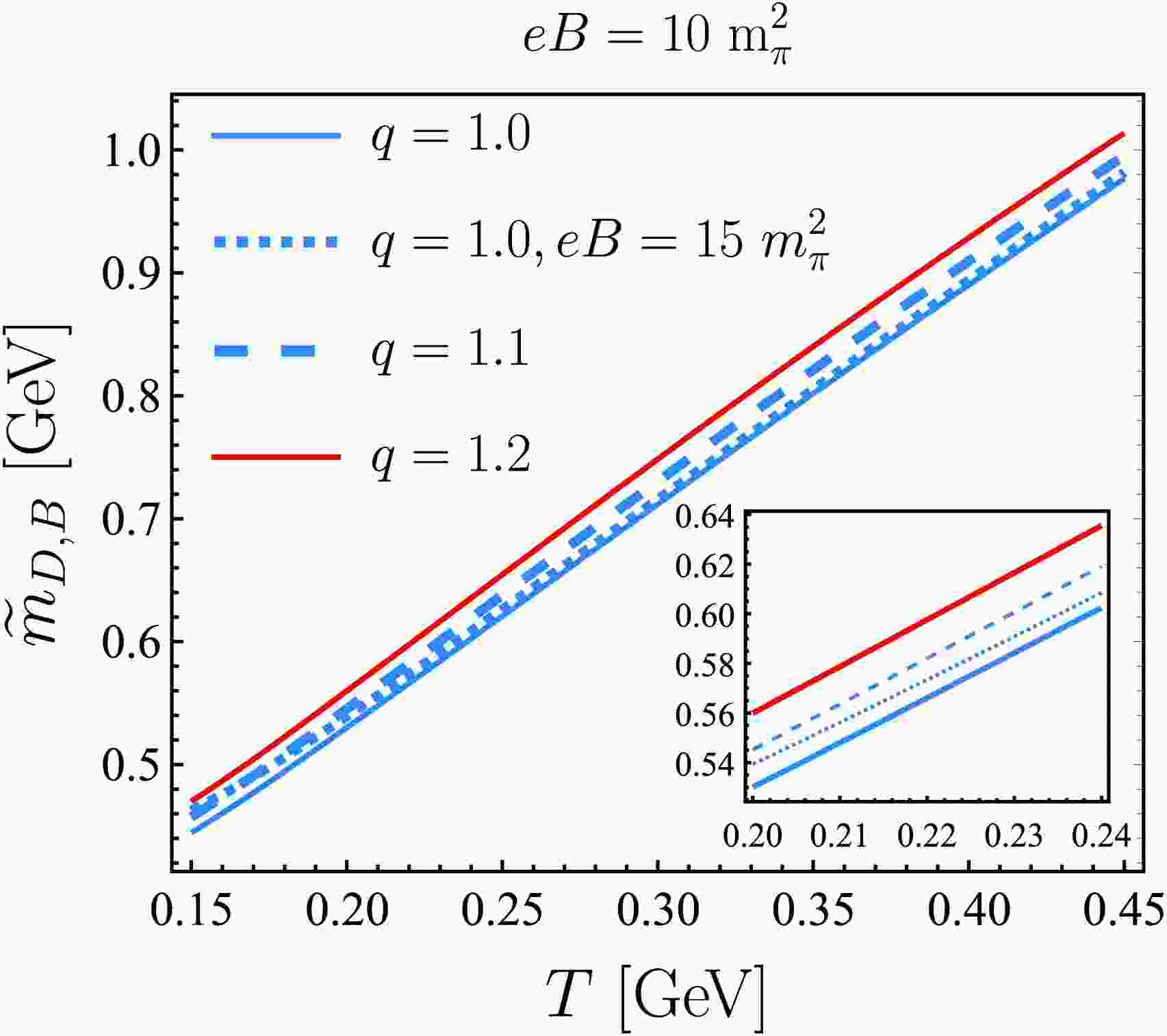
$ a_{R,B}^{\rm{quark}}=2(m_{D,R,B,(1)}^{\rm{quark}})^2/((q-1)(m_{D,B}^{\rm{quark}})^2) $ .In Fig. 1, we show the temperature dependence of the nonextensively modified Debye mass,
$ \widetilde{m}_{D,B} $ , at a magnetic field of$ eB=10\; m_{\pi}^2 $ . We observe that$ \widetilde{m}_{D,B} $ increases monotonically with both the temperature T and the nonextensive parameter q, implying that nonextensivity enhances color screening. The inset further shows that increasing the magnetic field strengthens the screening.
Figure 1. (color online) The temperature dependence of the Debye mass for different values of the nonextensive parameter q at
$ eB=10\; m_{\pi}^2 $ is shown. The dotted line represents the Debye mass at$ q=1 $ and$ eB=15\; m_{\pi}^2 $ .Next, we examine the quark contributions to the temporal component of the imaginary part of the retarded gluon self-energy,
$ \mathrm{Im}\,\Pi_{R}^{\rm{quark}} $ , in a finite magnetic field. In the static limit, the medium contribution to$ \mathrm{Im}\, \Pi_{R}^{\rm{quark}} $ for a nonextensive QGP is given by (see Appendix A for detailed derivations):$ \begin{aligned}[b] \underset{\omega\to 0}{\mathrm{lim}} \frac{ \mathrm{Im}\, \Pi^{\rm{quark}}_{R,{\rm{med}}}(Q)}{\omega} =\;& -\sum\limits_{f}\sum\limits_{n=1}^{\infty}\sum\limits_{b=\pm }\frac{g^2}{4\pi}\frac{2n|e_fB|^2}{TE_{\rho_z/2,n}^f|\rho_z|}\\&\times\bigg[\frac{qT\left(f_{q,FD}^{b}(E_{\rho_z/2,n}^f)\right)^2 }{{(E_{\rho_z,n}^f-b\mu)(q-1)+T}}\\ &\times\exp_q\bigg(\frac{E_{\rho_z/2,n}^f- b\mu}{T}\bigg)\bigg]. \end{aligned} $
(40) In the presence of small nonextensivity, the square-bracketed term in Eq. (40) is expanded to leading order in
$ (q-1) $ , yielding$ \Big[\dots \Big]\approx H_b^f(E_{\rho_z/2,n}^f)+\frac{q-1}{2}M_b^f(E_{\rho_z/2,n}^f). $
(41) By substituting Eq. (41) into Eq. (40) and adding the vacuum part of
$ \mathrm{Im}\, \Pi_{R}^{\rm{quark}} $ given in Eq. (A9), the static-limit ($ \omega\to 0 $ ) expression of$ \mathrm{Im}\, \Pi_{R}^{\rm{quark}} $ to order$ (q-1)^0 $ is given by$ \begin{aligned}[b] \underset{\omega\to 0}{\mathrm{lim}}\frac{\mathrm{Im}\, \Pi^{ {\rm{quark}} }_{R,(0)} (Q)}{\omega}=\;& - \sum\limits_{f}\sum\limits_{n=1}^{\infty}\sum\limits_{b=\pm}\frac{g^2}{4\pi} \frac{ 2n|e_fB|^2H^f_{b}(E^f_{\rho_z/2,n})}{TE_{\rho_z/2,n}^f|\rho_z|}\\& -\sum\limits_f\frac{g^2}{4\pi}|e_fB|\delta(\rho_z). \end{aligned} $
(42) To order
$ (q-1)^1 $ , we get$ \begin{aligned}[b] \underset{\omega\to 0}{\mathrm{lim}}\frac{\mathrm{Im}\,\Pi^{ {\rm{quark}} }_{R,(1) }(Q)}{\omega}=\;& - \sum\limits_{f}\sum\limits_{n=1}^{\infty}\sum\limits_{b=\pm}\frac{g^2}{4\pi} \frac{ 2n|e_fB|^2}{TE_{\rho_z/2,n}^f|\rho_z|}\\ & \times\frac{q-1}{2}M^f_{b}(E^f_{\rho_z/2,n}). \end{aligned}$
(43) By summing Eqs. (29), (32), (36), (37), (42), and (43), the temporal component of the total retarded gluon self-energy in the presence of a magnetic field, with the non-extensive correction included, is expressed as:
$ \begin{aligned}[b] \Pi_{R}(Q)=\;& \mathrm{Re}\,\Pi^{ \rm{quark }}_{R,(0)} (Q)+i\,\mathrm{Im }\,\Pi^{ \rm{quark }}_{R,(0)} (Q)\\& +\mathrm{Re}\,\Pi^{ \rm{quark }}_{R,(1)} (Q)+i\,\mathrm{Im }\,\Pi^{ \rm{quark }}_{R,(1)} (Q)\\& + \Pi_{R,(0)}^{\rm{gluon}}(Q)+\Pi_{R,(1)}^{\rm{gluon}}(Q). \end{aligned} $
(44) The one-loop quark contribution to the symmetric gluon self-energy in a finite magnetic field is medium-dependent and purely imaginary. Using Eqs. (A21-A23) from Appendix A, we have computed its temporal component in the static limit within nonextensive statistics, yielding:
$ \begin{aligned}[b] \underset{\omega\to 0}{\mathrm{lim}} \Pi^{\rm{quark}}_{F}(Q)=\;& -i\sum\limits_f\sum\limits_{n=1}^{\infty}\sum\limits_{b=\pm}\frac{g^2}{4\pi}\frac{8n|e_fB|^2}{E_{\rho_z/2,n}^f|\rho_z|}\\& \times f_{q,FD}^{b}(E_{\rho_z/2,n}^f)\left(1-f_{q,FD}^{b}(E_{\rho_z/2,n}^f)\right). \end{aligned} $
(45) If we consider only the leading-order non-extensive correction, the expression in square brackets above can be expanded as:
$\begin{aligned}[b] \big[\dots\big] \approx\;& H_{b}^f(E_{\rho_z/2,n}^f) \\&+f_{ q,FD,(1)}^{b}(E_{\rho_z/2,n}^f)\left[1-2f^{0b}_{FD}(E_{\rho_z/2,n}^f)\right]\\ & +{\cal{O}}(q-1)^2. \end{aligned}$
(46) Finally, to zeroth order in
$ (q-1) $ , Eq. (45) is obtained as follows:$ \underset{\omega\to 0}{\mathrm{lim}}\Pi^{\rm{quark }}_{F,(0)} (Q)=-i\sum\limits_{f}\sum\limits_{n=1}^{\infty}\sum\limits_{b=\pm}\frac{g^2}{4\pi} \frac{8n|e_fB|^2 H^f_{b} (E_{\rho_z/2,n}^f)}{E_{\rho_z/2,n}^f|\rho_z|}. $
(47) Correspondingly, the non-extensive correction term in Eq. (45), to order
$ (q-1)^1 $ , is expressed as$ \begin{aligned}[b] \underset{\omega\to 0}{\mathrm{lim}}\Pi^{\rm{quark}}_{F,(1)}(Q) =\;& -i\sum\limits_{f}\sum\limits_{n=1}^{\infty}\sum\limits_{b=\pm}\frac{g^2}{4\pi}\frac{8n|e_fB|^2 }{E_{\rho_z/2,n}^f|\rho_z|}\\ &\times\frac{q-1}{2}W^f_{b} (E_{\rho_z/2,n}^f), \end{aligned}$
(48) where the function
$ W_b^f(E_{\rho_z/2,n}^f) $ is defined as:$ \begin{aligned}[b] W_b^f(E_{\rho_z/2,n}^f) =\;& \frac{(E_{\rho_z/2,n}^f-b \mu)(E_{\rho_z/2,n}^f-b \mu-2T)}{T^2}\\ &\times\tanh\bigg(\frac{E_{\rho_z/2,n}^f-b \mu}{2T}\bigg) \\&\times H_b^f(E_{\rho_z/2,n}^f). \end{aligned} $
(49) Because gluons are electrically neutral, the one-loop gluon contribution to the symmetric gluon self-energy shows no explicit dependence on the magnetic field. In the HTL approximation, the one-loop contribution from gluons to the temporal component of the symmetric gluon self-energy, denoted by
$ \Pi_{F}^{\rm{gluon}} $ , has been computed in non-extensive statistics [89] and is expressed as:$ \begin{aligned}[b]\Pi^{\rm{gluon}}_F(Q)=\;& -ig^2\int \frac{dk k^{2}}{2\pi}2N_{c}f_{q,BE} (k)(1+f_{q,BE} (k))\\& \times\frac{2}{\rho}\Theta(\rho^{2}-\omega^{2}). \end{aligned} $
(50) To order
$ (q-1)^0 $ , Eq. (50) simplifies to:$ \Pi^{\rm{gluon}}_{F,(0)}(Q) = -2\pi i (m_{D,F}^{\rm{gluon}})^2 \frac{T}{\rho}\Theta(\rho^{2}-\omega^{2}), $
(51) where
$ m_{D,F}^{\rm{gluon}}=m_{D}^{\rm{gluon}} $ is the conventional Debye mass arising from the gluon-loop contribution in standard quantum statistics. The leading-order non-extensive correction in$ (q-1) $ to$ \Pi_{F}^{\rm{gluon}} $ is computed as follows:$ \begin{aligned}[b] \Pi^{\rm{gluon}}_{F,(1)}(Q)= \;&-ig^2\int \frac{dk k^{2}}{2\pi} 2N_cf_{q,BE,(1)} (k)(1+2f_{BE}^0 (k))\\& \times\frac{2}{\rho}\Theta(\rho^{2}-\omega^{2})\\ =\;& -2\pi i (m_{D,F,(1)}^{\rm{gluon}})^2\frac{T}{\rho}\Theta(\rho^{2}-\omega^{2}). \end{aligned} $
(52) Here,
$ m_{D,F,(1)}^{\rm{gluon}}= (m_{D}^{\rm{gluon}})^2\dfrac{q-1}{2}a^{\rm{gluon}}_{F} $ denotes the leading-order non-extensive correction term arising from the gluon-loop contribution to the symmetric Debye mass, where the dimensionless quantity$ a^{\rm{gluon}}_{F} $ is defined as:$ \begin{aligned}[b] a^{\rm{gluon}}_{F}=\;& \frac{2}{q-1} \frac{\displaystyle\int dk \ k^2 f_{q,BE,(1)}(k) (1 +2 f^0_{BE} (k) ) }{ \displaystyle\int dk\ k^2 f^0_{BE} (k) ( 1 +f^0_{BE} (k) )}\\ =\;& \frac{72 }{\pi^{2}}\zeta(3)-6. \end{aligned} $
(53) By inserting Eq. (29) and Eq. (36) into Eq. (22), we obtain the temporal component of the resummed retarded gluon propagator to order
$ (q-1)^0 $ , denoted by$ G^*_{R,(0)} $ . In the static limit$ (\omega\to 0) $ , it is expressed as:$ \begin{aligned}[b] \underset{\omega\to 0}{\mathrm{lim}}G^*_{R,(0)}(Q)=\;& \frac{1}{{\rho}^2+{m}_{D,B}^2}+\frac{\underset{\omega\to 0}{\mathrm{lim}}\mathrm{Im}\,\Pi_{R,(0)}^{\rm{quark}}(Q)}{(\rho^2+m_{D,B}^2)^2}\\& -i\frac{\omega\pi ({m}_{D}^{\rm{gluon}})^2}{2\rho({\rho}^2+{m}_{D,B}^2)^2}. \end{aligned} $
(54) By inserting Eqs. (29), (32), (36), and (37) into Eq. (23), the leading-order non-extensive corrections to the temporal component of the resummed retarded gluon propagator, associated with the quark-loop and gluon contributions to the self-energy and denoted by
$ G^{* {\rm{quark}}}_{R,(1)} $ and$ G^{* {\rm{gluon}}}_{R,(1)} $ , are determined. In the static limit ($ \omega\to 0 $ ), they are respectively expressed as$ \begin{aligned}[b] \underset{\omega\to 0}{\mathrm{lim}}G^{* {\rm{gluon}}}_{R,(1)}(Q)=\;& \underset{\omega\to 0}{\mathrm{lim}}\frac{\Pi^{\rm{gluon}}_{R,(1)}(Q)}{\left(G_{R}^{-1}(Q)-\Pi_{R,(0)}(Q)\right)^2}\\=\;& -\frac{(m_{D,R,(1)}^{\rm{gluon}})^2}{({\rho}^2+{m}_{D,B}^2)^2}\\&+i\frac{\omega \pi ({m}_{D,R,(1)}^{\rm{gluon}})^2(m_{D}^{\rm{gluon}})^2}{\rho({\rho}^2+{m}_{D,B}^2)^3}\\&-i\frac{2({m}_{D,R,(1)}^{\rm{gluon}})^2\underset{\omega\to 0}{\mathrm{lim}}\mathrm{Im}\, \Pi_{R,(0)}^{\rm{quark}}}{({\rho}^2+{m}_{D,B}^2)^3}\\ & -i\frac{\omega\pi ({m}_{D,R,(1)}^{\rm{gluon}})^2}{2\rho({\rho}^2+{m}_{D,B}^2)^2}, \end{aligned} $
(55) and
$ \begin{aligned}[b] \underset{\omega\to 0}{\mathrm{lim}}G^{* {\rm{quark}}}_{R,(1)}(Q)=\;& \underset{\omega\to 0}{\mathrm{lim}}\frac{\Pi^{\rm{quark}}_{R,(1)}(Q)}{\left(G_{R}^{-1}(Q)-\Pi_{R,(0)}(Q)\right)^2}\\=\;& -\frac{(m_{D,R,B,(1)}^{\rm{quark}})^2}{({\rho}^2+m_{D,B}^2)^2}\\& +i\frac{\omega\pi (m_{D,R,B,(1)}^{\rm{quark}})^2(m_{D}^{\rm{gluon}})^2}{\rho(\rho^2+m_{D,B}^2)^3}\\& -i\frac{2(m_{D,R,B,(1)}^{\rm{quark}})^2\underset{\omega\to 0}{\mathrm{lim}}\mathrm{Im}\,\Pi_{R,(0)}^{\rm{quark}}(Q)}{(\rho^2+m_{D,B}^2)^3}\\& +i\frac{\underset{\omega\to 0}{\mathrm{lim}}\mathrm{Im}\,\Pi_{R,(1)}^{\rm{quark}}(Q)}{(\rho^2+m_{D,B}^2)^2}. \end{aligned} $
(56) In Eqs. (54-56), we retain the first-order (in ω) imaginary part of the resummed retarded gluon propagator to derive the symmetric resummed gluon propagator. Similarly, by inserting Eqs. (29), (36), (42), (47), (51) and (54) into Eq. (25), we obtain the temporal component of the resummed symmetric gluon propagator at order
$ (q-1)^0 $ in the magnetic field, denoted by$ G_{F,(0)}^{*} $ . In the static limit ($ \omega\to 0 $ ), it is given by$ \begin{aligned}[b]\underset{\omega\to 0}{\mathrm{lim}}G_{F,(0)}^{*\rm}(Q)=\;& -i\frac{2T\pi ({m}_{D}^{\rm{gluon}})^2}{\rho({\rho}^2+m_{D,B}^2)^2} \\&+\frac{\underset{\omega\to 0}{\mathrm{lim}} \Pi_{F,(0)}^{\rm{quark}}(Q)}{(\rho^2+m_{D,B}^2)^2} . \end{aligned} $
(57) By substituting Eqs. (36), (37), (42), (43), (47), (48), (51), (52), (54), and (58) into Eq. (26), one finally obtains the non-extensive correction to the temporal component of the resummed symmetric gluon propagator, arising from gluon-loop and quark-loop contributions to the self-energy at order
$ (q-1)^1 $ in a finite magnetic field, denoted by$ G_{F,(1)}^{*{\rm{quark}}} $ and$ G_{F,(1)}^{*{\rm{gluon}}} $ . In the static limit ($ \omega\to 0 $ ), they are expressed, respectively, as$ \begin{aligned}[b] \underset{\omega\to 0}{\mathrm{lim}}G_{F,(1)}^{* {\rm{gluon}}}(Q) =\;& i\frac{4T\pi ({m}_{D,R,(1)}^{\rm{gluon}})^2}{\rho({\rho}^2+{m}_{D,B}^2)^3}(m_{D}^{\rm{gluon}})^2\\& -i\frac{8T({m}_{D,R,(1)}^{\rm{gluon}})^2}{({\rho}^2+{m}_{D,B}^2)^3}\frac{\underset{\omega\to 0}{\mathrm{lim}}\mathrm{Im}\, \Pi_{R,(0)}^{\rm{quark}}(Q)}{\omega}\\ & -i\frac{2T\pi (m_{D,F,(1)}^{\rm{gluon}})^2 }{\rho(\rho^2+m_{D,B}^2)^2}, \end{aligned} $
(58) and
$ \begin{aligned}[b]\underset{\omega\to 0}{\mathrm{lim}}G_{F,(1)}^{* {\rm{quark}}}(Q) = \;&i\frac{4T\pi (m_{D,R,(1)}^{\rm{quark}})^2(m_{D}^{\rm{gluon}})^2}{\rho(\rho^2+m_{D,B}^2)^3}\\& -i\frac{8T(m_{D,R,B,(1)}^{\rm{quark}})^2}{(\rho^2+m_{D,B}^2)^3}\frac{\underset{\omega\to 0}{\mathrm{lim}}\mathrm{Im}\,\Pi_{R,(0)}^{\rm{quark}}(Q)}{\omega}\\ & +\frac{\underset{\omega\to 0}{\mathrm{lim}}\Pi_{F,(1)}^{\rm{quark}}(Q)}{(\rho^2+m_{D,B}^2)^2}. \end{aligned} $
(59) -
In the presence of a magnetic field, Landau quantization of light quarks significantly modifies the quark-loop contribution to the gluon self-energy, leading to results that differ markedly from the zero-field case. Moreover, in contrast to the HTL approximation in
$ (3+1) $ dimensions, the quark-loop contribution to the vacuum part of the temporal component of the retarded gluon self-energy in a finite magnetic field, denoted by$ \Pi_{R,\rm vac}^{\rm{quark}} $ , persists even at high temperature and/or density, as presented in Eq. (A9). To gain a deeper understanding of the gluon self-energy, we separate the calculations of its real and imaginary parts. In the HTL approximation within the hierarchy of scales$ T^2\sim eB\gg g^2T^2 $ [19, 34], we calculate the one-loop quark contribution to the medium part of the temporal component of the retarded gluon self-energy in a finite magnetic field, denoted by$ \Pi_{R,{\rm{med}}}^{\rm{quark}} $ . The detailed derivation is presented in Appendix A. Subsequently, its real part in the static limit ($ \omega\to0 $ ) is written as$ \begin{aligned}[b] \underset{\omega\to 0}{\mathrm{lim}} \mathrm{Re}\, \Pi_{R,{\rm{med}}}^{\rm{quark}}(Q)= \sum\limits_f\sum\limits_{n=1}^{\infty}\sum\limits_{b=\pm }\frac{g^2|e_fB|\alpha_{0n}}{4\pi} \int\frac{{\mathrm{d}}k_z }{2\pi}\Bigg\{\frac{2(E^f_{k_z,n})^2+\rho_zk_z}{E_{k_z,n}^f[(E_{k_z,n}^f)^2-(E_{p_z,n}^f)^2]}f^{b}_{q,FD}(E_{k_z,n}^f) +\frac{(E^f_{p_z,n})^2+(E^f_{k_z,n})^2+\rho_zk_z}{E_{p_z,n}^f[(E_{p_z,n}^f)^2-(E_{k_z,n}^f)^2]}f^{b}_{q,FD}(E_{p_z,n}^f)\Bigg\}, \end{aligned} $
(27) where
$ Q = (\omega, {{\rho}}) $ denotes the external four-momentum in the one-loop diagram and corresponds to a soft scale;$ E_{p_z,n}^f=\sqrt{p_z^2+2n|e_fB|} $ , with$ p_z=k_z+\rho_z $ . The factor$ \alpha_{0n}=(2-\delta_{0,n}) $ is the Landau-level-dependent spin degeneracy. Note that the summation over Landau levels in the above equation starts at$ n=1 $ rather than$ n=0 $ because the one-loop contribution from the lowest Landau level quarks to the medium part of the retarded self-energy vanishes; see AppendixA for details.In the HTL approximation, since
$ \rho_z/k_z $ is a small quantity, we can expand the term in curly brackets in Eq. (27) as a power series in$ \rho_z/k_z $ :$\begin{aligned}[b] \bigg\{\dots\bigg\}\approx \;&\frac{H_{b}^f(E^f_{k_z,n})+ f_{q,FD,(1)}^{b}(E_{k_z,n}^f)(1-2f^{0b }_{FD}(E_{k_z,n}^f))}{T}\\& -\frac{1}{T^2}(q-1)(E_{k_z,n}^f-b \mu)H_{b }^f(E^f_{k_z,n}) \\& +\frac{1}{T}(q-1)H_{b}^f(E^f_{k_z,n})+{\cal{O}}(\frac{\rho_z}{k_z}). \end{aligned} $
(28) Here,
$ H_{b}^f(E^f_{k_z,n})=f^{0b}_{FD}(E^f_{k_z,n})(1-f^{0b}_{FD}(E^f_{k_z,n})) $ . By summing the real parts given in Eq. (A9) and Eq. (27), we obtain the total real part of the one-loop quark contribution to the temporal component of the retarded gluon self-energy in a finite magnetic field, denoted by$ \mathrm{Re}\,\Pi_{R}^{\rm{quark}} $ . In the static limit ($ \omega\to 0 $ ), to order$ (q-1)^0 $ , it can be expressed as$\begin{aligned}[b] \underset{\omega\to 0}{\mathrm{lim}} \mathrm{Re}\, \Pi_{R,(0)}^{\rm{quark}}(Q) =\;& -\sum\limits_{f}\sum\limits_{n=0}\limits^{\infty}\sum\limits_{b=\pm }\frac{g^2\alpha_{0n}|e_fB|}{4\pi T}\\& \times\int\frac{{\mathrm{d}}k_z}{2\pi}H_{b}^f(E^f_{k_z,n}).\end{aligned} $
(29) We emphasize that the Landau-level summation in Eq. (29) starts at
$ n=0 $ to include the real part of$ \Pi_{R,\mathrm{vac}}^{\mathrm{quark}} $ (Eq. (A9)), which, in the static limit, can be rewritten as:$ \begin{aligned}[b] \underset{\omega\to 0}{\mathrm{lim}}\mathrm{Re}\,\Pi_{R,\rm vac}^{\rm{quark}}(Q)=\;& -\sum\limits_f\frac{g^2|e_fB|}{4\pi^2}\\ =\;& -\sum\limits_{f}\sum\limits_{b=\pm} \frac{g^2|e_fB|}{4\pi T}\int\frac{{\mathrm{d}}k_z}{2\pi}H_b^f(|k_z|). \end{aligned} $
(30) Eq. (29) simply gives the standard Debye mass from the quark contribution in a finite magnetic field, i.e.,
$ (m_{D,B}^{\rm{quark}})^2=-\underset{\omega\to 0}{\mathrm{lim}} \mathrm{Re}\,\Pi_{R,(0)}^{\rm{quark}}(Q) $ . Since thermal gluons are not directly affected by the magnetic field, the computation of the one-loop gluon contribution to the gluon self-energy in the presence of a magnetic field is identical to that in its absence. Therefore, within standard quantum statistics, the total magnetic-field-dependent Debye mass from the retarded/advanced gluon self-energy is given as$ m_{D,B}^2=(m_{D,B}^{\rm{quark}})^2+(m_{D}^{\rm{gluon}})^2, $
(31) This is also consistent with the result obtained using semiclassical transport theory in a magnetic field [87].
By inserting Eq. (28) into Eq. (27), we obtain the leading-order non-extensive correction (in
$ (q-1) $ ) to$ \mathrm{Re}\,\Pi_{R}^{\rm{quark}} $ , denoted by$ \mathrm{Re}\, \Pi_{R,(1)}^{\rm{quark}} $ . In the static limit ($ \omega\to 0 $ ), it is expressed as$ \begin{aligned}[b] \underset{\omega\to 0}{\mathrm{lim}} \mathrm{Re}\,\Pi^{\rm{quark}}_{R,(1)}(Q) =\;& -\sum\limits_{f}\sum\limits_{n=1}\limits^{\infty}\sum\limits_{b=\pm }\frac{g^2|e_fB|}{4\pi^2 T}\\&\times \int {\mathrm{d}}k_z\frac{(q-1)}{2}M_{b}^f(E^f_{k_z,n}), \end{aligned} $
(32) where the function
$ M_b^f(E_{k_z,n}^f) $ is defined as:$ \begin{aligned}[b] M^{f}_b(E_{k_z,n}^f)=\;& H_{b}^f(E_{k_z,n}^f)\frac{(E_{k_z,n}^f-b \mu)}{T}\\& \times\bigg[\frac{(E_{k_z,n}^f-b \mu-2T)}{T}\tanh\left(\frac{E_{k_z,n}^f-b \mu}{2T}\right)\\&-2+\frac{2T}{(E_{k_z,n}^f-b \mu)}\bigg]. \end{aligned} $
(33) Correspondingly, we derive the nonextensive correction to the retarded Debye mass from quark contributions in a finite magnetic field given by:
$ (m_{D,R,B,(1)}^{\rm{quark}})^2= - \underset{\omega\to 0}{\mathrm{lim}} \mathrm{Re}\,\Pi^{\rm{quark}}_{R,(1)}(Q). $
(34) In the HTL approximation, the one-loop gluonic contributions to the temporal component of the retarded gluon self-energy, denoted by
$ \Pi_{R} $ , computed within non-extensive statistics take the form [82, 88, 89]:$ \begin{aligned}[b] \Pi_{R}^{\rm{gluon}}(Q)=\;& \frac{ g^2}{(2\pi)^3}\int k{\mathrm{d}}k\frac{{\mathrm{d}}\Omega_k}{2} \left(2N_c f_{q,BE}(k)\right)\\ & \times\bigg[\frac{1-x^2}{[x+(\omega+{\mathrm{i}}\epsilon)/\rho]^2}\\ & +\frac{1-x^2}{[-x+(\omega+{\mathrm{i}}\epsilon)/\rho]^2}\bigg]. \end{aligned} $
(35) The differential solid angle is given by
$ \mathrm{d}\Omega_k=\sin\theta\mathrm{d}\theta\mathrm{d}\phi= \mathrm{d}x\mathrm{d}\phi $ , where$ x={{k}}\cdot{{\rho}}/(k\rho) $ and$ \rho\equiv |{{\rho}}| $ . At order$ (q-1)^0 $ , Eq. (35) simplifies to:$ \Pi^{\rm{gluon}}_{R,(0)}(Q) =( m_{D}^{\rm{gluon}})^2\left(\frac{\omega}{2\rho}\ln\frac{\omega+\rho+ {\mathrm{i}}\epsilon}{\omega-\rho+ {\mathrm{i}}\epsilon}-1\right). $
(36) In Eq. (36),
$ m_{D}^{\rm{gluon}} $ represents the gluon-loop contribution to the Debye mass in standard quantum statistics and is given by$ (m_{D}^{\rm{gluon}})^2=\dfrac{g^{2}T^{2}}{3}N_{c} $ .In the presence of nonextensivity, the leading-order nonextensive correction to
$ \Pi_{R}^{\rm{gluon}}(Q) $ , denoted by$ \Pi_{R,(1)}(Q) $ , is given by:$ \begin{aligned}[b] \Pi^{\rm{gluon}}_{R,(1)}(Q) =\;& \frac{ g^2}{\pi^2}\int k{\mathrm{d}}k \left( 2N_c f_{q,BE,(1)}(k)\right)\\& \times\left(\frac{\omega}{2\rho}\ln\frac{\omega+\rho+{\mathrm{i}}\epsilon}{\omega-\rho+ {\mathrm{i}}\epsilon}-1\right) \\ =\;& (m_{D,R,(1)}^{\rm{gluon}})^{2}\left(\frac{\omega}{2\rho}\ln\frac{\omega+\rho+ {\mathrm{i}}\epsilon}{\omega-\rho+ {\mathrm{i}}\epsilon}-1\right). \end{aligned} $
(37) Here,
$ (m_{D,R,(1)}^{\rm{gluon}})^2=\dfrac{q-1}{2}(m_{D}^{\rm{gluon}})^2a^{\rm{gluon}}_{R} $ denotes the non-extensive correction to the retarded Debye mass from the gluon-loop contribution, where the dimensionless quantity$ a^{\rm{gluon}}_{R} $ is defined as:$ a^{\rm{gluon}}_{R} = \frac{2}{(q-1)} \frac{\int k {\mathrm{d}}k f_{q,BE,(1)}(k)}{\int k {\mathrm{d}}k f^0_{BE}(k)}=\frac{36}{\pi^2}\zeta(3)-4. $
(38) Finally, the total non-extensive, modified retarded Debye mass in the presence of a magnetic field is given by:
$ \begin{aligned}[b] \widetilde{m}_{D,B}^2=\;& \widetilde{m}_{D,R,B}^2 =(m_{D,B}^{\rm{quark}})^2\left(1+\frac{q-1}{2}a_{R,B}^{\rm{quark}}\right)\\ & +(m_{D}^{\rm{gluon}})^2 \left(1+\frac{q-1}{2}a^{\rm{gluon}}_{F}\right), \end{aligned}$
(39) with the corresponding dimensionless quantity being
$ a_{R,B}^{\rm{quark}}=2(m_{D,R,B,(1)}^{\rm{quark}})^2/((q-1)(m_{D,B}^{\rm{quark}})^2) $ .In Fig. 1, we show the temperature dependence of the nonextensively modified Debye mass,
$ \widetilde{m}_{D,B} $ , at a magnetic field of$ eB=10\; m_{\pi}^2 $ . We observe that$ \widetilde{m}_{D,B} $ increases monotonically with both the temperature T and the nonextensive parameter q, implying that nonextensivity enhances color screening. The inset further shows that increasing the magnetic field strengthens the screening.
Figure 1. (color online) The temperature dependence of the Debye mass for different values of the nonextensive parameter q at
$ eB=10\; m_{\pi}^2 $ is shown. The dotted line represents the Debye mass at$ q=1 $ and$ eB=15\; m_{\pi}^2 $ .Next, we examine the quark contributions to the temporal component of the imaginary part of the retarded gluon self-energy,
$ \mathrm{Im}\,\Pi_{R}^{\rm{quark}} $ , in a finite magnetic field. In the static limit, the medium contribution to$ \mathrm{Im}\, \Pi_{R}^{\rm{quark}} $ for a nonextensive QGP is given by (see Appendix A for detailed derivations):$ \begin{aligned}[b] \underset{\omega\to 0}{\mathrm{lim}} \frac{ \mathrm{Im}\, \Pi^{\rm{quark}}_{R,{\rm{med}}}(Q)}{\omega} =\;& -\sum\limits_{f}\sum\limits_{n=1}^{\infty}\sum\limits_{b=\pm }\frac{g^2}{4\pi}\frac{2n|e_fB|^2}{TE_{\rho_z/2,n}^f|\rho_z|}\\&\times\bigg[\frac{qT\left(f_{q,FD}^{b}(E_{\rho_z/2,n}^f)\right)^2 }{{(E_{\rho_z,n}^f-b\mu)(q-1)+T}}\\ &\times\exp_q\bigg(\frac{E_{\rho_z/2,n}^f- b\mu}{T}\bigg)\bigg]. \end{aligned} $
(40) In the presence of small nonextensivity, the square-bracketed term in Eq. (40) is expanded to leading order in
$ (q-1) $ , yielding$ \Big[\dots \Big]\approx H_b^f(E_{\rho_z/2,n}^f)+\frac{q-1}{2}M_b^f(E_{\rho_z/2,n}^f). $
(41) By substituting Eq. (41) into Eq. (40) and adding the vacuum part of
$ \mathrm{Im}\, \Pi_{R}^{\rm{quark}} $ given in Eq. (A9), the static-limit ($ \omega\to 0 $ ) expression of$ \mathrm{Im}\, \Pi_{R}^{\rm{quark}} $ to order$ (q-1)^0 $ is given by$ \begin{aligned}[b] \underset{\omega\to 0}{\mathrm{lim}}\frac{\mathrm{Im}\, \Pi^{ {\rm{quark}} }_{R,(0)} (Q)}{\omega}=\;& - \sum\limits_{f}\sum\limits_{n=1}^{\infty}\sum\limits_{b=\pm}\frac{g^2}{4\pi} \frac{ 2n|e_fB|^2H^f_{b}(E^f_{\rho_z/2,n})}{TE_{\rho_z/2,n}^f|\rho_z|}\\& -\sum\limits_f\frac{g^2}{4\pi}|e_fB|\delta(\rho_z). \end{aligned} $
(42) To order
$ (q-1)^1 $ , we get$ \begin{aligned}[b] \underset{\omega\to 0}{\mathrm{lim}}\frac{\mathrm{Im}\,\Pi^{ {\rm{quark}} }_{R,(1) }(Q)}{\omega}=\;& - \sum\limits_{f}\sum\limits_{n=1}^{\infty}\sum\limits_{b=\pm}\frac{g^2}{4\pi} \frac{ 2n|e_fB|^2}{TE_{\rho_z/2,n}^f|\rho_z|}\\ & \times\frac{q-1}{2}M^f_{b}(E^f_{\rho_z/2,n}). \end{aligned}$
(43) By summing Eqs. (29), (32), (36), (37), (42), and (43), the temporal component of the total retarded gluon self-energy in the presence of a magnetic field, with the non-extensive correction included, is expressed as:
$ \begin{aligned}[b] \Pi_{R}(Q)=\;& \mathrm{Re}\,\Pi^{ \rm{quark }}_{R,(0)} (Q)+{\mathrm{i}}\,\mathrm{Im }\,\Pi^{ \rm{quark }}_{R,(0)} (Q)\\& +\mathrm{Re}\,\Pi^{ \rm{quark }}_{R,(1)} (Q)+{\mathrm{i}}\,\mathrm{Im }\,\Pi^{ \rm{quark }}_{R,(1)} (Q)\\& + \Pi_{R,(0)}^{\rm{gluon}}(Q)+\Pi_{R,(1)}^{\rm{gluon}}(Q). \end{aligned} $
(44) The one-loop quark contribution to the symmetric gluon self-energy in a finite magnetic field is medium-dependent and purely imaginary. Using Eqs. (A21-A23) from Appendix A, we have computed its temporal component in the static limit within nonextensive statistics, yielding:
$ \begin{aligned}[b] \underset{\omega\to 0}{\mathrm{lim}} \Pi^{\rm{quark}}_{F}(Q)=\;& -{\mathrm{i}}\sum\limits_f\sum\limits_{n=1}^{\infty}\sum\limits_{b=\pm}\frac{g^2}{4\pi}\frac{8n|e_fB|^2}{E_{\rho_z/2,n}^f|\rho_z|}\\& \times f_{q,FD}^{b}(E_{\rho_z/2,n}^f)\left(1-f_{q,FD}^{b}(E_{\rho_z/2,n}^f)\right). \end{aligned} $
(45) If we consider only the leading-order non-extensive correction, the expression in square brackets above can be expanded as:
$\begin{aligned}[b] \big[\dots\big] \approx\;& H_{b}^f(E_{\rho_z/2,n}^f) \\&+f_{ q,FD,(1)}^{b}(E_{\rho_z/2,n}^f)\left[1-2f^{0b}_{FD}(E_{\rho_z/2,n}^f)\right]\\ & +{\cal{O}}(q-1)^2. \end{aligned}$
(46) Finally, to zeroth order in
$ (q-1) $ , Eq. (45) is obtained as follows:$ \underset{\omega\to 0}{\mathrm{lim}}\Pi^{\rm{quark }}_{F,(0)} (Q)=-{\mathrm{i}}\sum\limits_{f}\sum\limits_{n=1}^{\infty}\sum\limits_{b=\pm}\frac{g^2}{4\pi} \frac{8n|e_fB|^2 H^f_{b} (E_{\rho_z/2,n}^f)}{E_{\rho_z/2,n}^f|\rho_z|}. $
(47) Correspondingly, the non-extensive correction term in Eq. (45), to order
$ (q-1)^1 $ , is expressed as$ \begin{aligned}[b] \underset{\omega\to 0}{\mathrm{lim}}\Pi^{\rm{quark}}_{F,(1)}(Q) =\;& -{\mathrm{i}}\sum\limits_{f}\sum\limits_{n=1}^{\infty}\sum\limits_{b=\pm}\frac{g^2}{4\pi}\frac{8n|e_fB|^2 }{E_{\rho_z/2,n}^f|\rho_z|}\\ &\times\frac{q-1}{2}W^f_{b} (E_{\rho_z/2,n}^f), \end{aligned}$
(48) where the function
$ W_b^f(E_{\rho_z/2,n}^f) $ is defined as:$ \begin{aligned}[b] W_b^f(E_{\rho_z/2,n}^f) =\;& \frac{(E_{\rho_z/2,n}^f-b \mu)(E_{\rho_z/2,n}^f-b \mu-2T)}{T^2}\\ &\times\tanh\bigg(\frac{E_{\rho_z/2,n}^f-b \mu}{2T}\bigg) \\&\times H_b^f(E_{\rho_z/2,n}^f). \end{aligned} $
(49) Because gluons are electrically neutral, the one-loop gluon contribution to the symmetric gluon self-energy shows no explicit dependence on the magnetic field. In the HTL approximation, the one-loop contribution from gluons to the temporal component of the symmetric gluon self-energy, denoted by
$ \Pi_{F}^{\rm{gluon}} $ , has been computed in non-extensive statistics [89] and is expressed as:$ \begin{aligned}[b]\Pi^{\rm{gluon}}_F(Q)=\;& -{\mathrm{i}}g^2\int \frac{{\mathrm{d}}k k^{2}}{2\pi}2N_{c}f_{q,BE} (k)(1+f_{q,BE} (k))\\& \times\frac{2}{\rho}\Theta(\rho^{2}-\omega^{2}). \end{aligned} $
(50) To order
$ (q-1)^0 $ , Eq. (50) simplifies to:$ \Pi^{\rm{gluon}}_{F,(0)}(Q) = -2\pi {\mathrm{i}} (m_{D,F}^{\rm{gluon}})^2 \frac{T}{\rho}\Theta(\rho^{2}-\omega^{2}), $
(51) where
$ m_{D,F}^{\rm{gluon}}=m_{D}^{\rm{gluon}} $ is the conventional Debye mass arising from the gluon-loop contribution in standard quantum statistics. The leading-order non-extensive correction in$ (q-1) $ to$ \Pi_{F}^{\rm{gluon}} $ is computed as follows:$ \begin{aligned}[b] \Pi^{\rm{gluon}}_{F,(1)}(Q)= \;&-{\mathrm{i}}g^2\int \frac{{\mathrm{d}}k k^{2}}{2\pi} 2N_cf_{q,BE,(1)} (k)(1+2f_{BE}^0 (k))\\& \times\frac{2}{\rho}\Theta(\rho^{2}-\omega^{2})\\ =\;& -2\pi {\mathrm{i}} (m_{D,F,(1)}^{\rm{gluon}})^2\frac{T}{\rho}\Theta(\rho^{2}-\omega^{2}). \end{aligned} $
(52) Here,
$ m_{D,F,(1)}^{\rm{gluon}}= (m_{D}^{\rm{gluon}})^2\dfrac{q-1}{2}a^{\rm{gluon}}_{F} $ denotes the leading-order non-extensive correction term arising from the gluon-loop contribution to the symmetric Debye mass, where the dimensionless quantity$ a^{\rm{gluon}}_{F} $ is defined as:$ \begin{aligned}[b] a^{\rm{gluon}}_{F}=\;& \frac{2}{q-1} \frac{\displaystyle\int {\mathrm{d}}k \ k^2 f_{q,BE,(1)}(k) (1 +2 f^0_{BE} (k) ) }{ \displaystyle\int {\mathrm{d}}k\ k^2 f^0_{BE} (k) ( 1 +f^0_{BE} (k) )}\\ =\;& \frac{72 }{\pi^{2}}\zeta(3)-6. \end{aligned} $
(53) By inserting Eq. (29) and Eq. (36) into Eq. (22), we obtain the temporal component of the resummed retarded gluon propagator to order
$ (q-1)^0 $ , denoted by$ G^*_{R,(0)} $ . In the static limit$ (\omega\to 0) $ , it is expressed as:$ \begin{aligned}[b] \underset{\omega\to 0}{\mathrm{lim}}G^*_{R,(0)}(Q)=\;& \frac{1}{{\rho}^2+{m}_{D,B}^2}+\frac{\underset{\omega\to 0}{\mathrm{lim}}\mathrm{Im}\,\Pi_{R,(0)}^{\rm{quark}}(Q)}{(\rho^2+m_{D,B}^2)^2}\\& -{\mathrm{i}}\frac{\omega\pi ({m}_{D}^{\rm{gluon}})^2}{2\rho({\rho}^2+{m}_{D,B}^2)^2}. \end{aligned} $
(54) By inserting Eqs. (29), (32), (36), and (37) into Eq. (23), the leading-order non-extensive corrections to the temporal component of the resummed retarded gluon propagator, associated with the quark-loop and gluon contributions to the self-energy and denoted by
$ G^{* {\rm{quark}}}_{R,(1)} $ and$ G^{* {\rm{gluon}}}_{R,(1)} $ , are determined. In the static limit ($ \omega\to 0 $ ), they are respectively expressed as$ \begin{aligned}[b] \underset{\omega\to 0}{\mathrm{lim}}G^{* {\rm{gluon}}}_{R,(1)}(Q)=\;& \underset{\omega\to 0}{\mathrm{lim}}\frac{\Pi^{\rm{gluon}}_{R,(1)}(Q)}{\left(G_{R}^{-1}(Q)-\Pi_{R,(0)}(Q)\right)^2}\\=\;& -\frac{(m_{D,R,(1)}^{\rm{gluon}})^2}{({\rho}^2+{m}_{D,B}^2)^2}\\&+{\mathrm{i}}\frac{\omega \pi ({m}_{D,R,(1)}^{\rm{gluon}})^2(m_{D}^{\rm{gluon}})^2}{\rho({\rho}^2+{m}_{D,B}^2)^3}\\&-{\mathrm{i}}\frac{2({m}_{D,R,(1)}^{\rm{gluon}})^2\underset{\omega\to 0}{\mathrm{lim}}\mathrm{Im}\, \Pi_{R,(0)}^{\rm{quark}}}{({\rho}^2+{m}_{D,B}^2)^3}\\ & -{\mathrm{i}}\frac{\omega\pi ({m}_{D,R,(1)}^{\rm{gluon}})^2}{2\rho({\rho}^2+{m}_{D,B}^2)^2}, \end{aligned} $
(55) and
$ \begin{aligned}[b] \underset{\omega\to 0}{\mathrm{lim}}G^{* {\rm{quark}}}_{R,(1)}(Q)=\;& \underset{\omega\to 0}{\mathrm{lim}}\frac{\Pi^{\rm{quark}}_{R,(1)}(Q)}{\left(G_{R}^{-1}(Q)-\Pi_{R,(0)}(Q)\right)^2}\\=\;& -\frac{(m_{D,R,B,(1)}^{\rm{quark}})^2}{({\rho}^2+m_{D,B}^2)^2}\\& +{\mathrm{i}}\frac{\omega\pi (m_{D,R,B,(1)}^{\rm{quark}})^2(m_{D}^{\rm{gluon}})^2}{\rho(\rho^2+m_{D,B}^2)^3}\\& -{\mathrm{i}}\frac{2(m_{D,R,B,(1)}^{\rm{quark}})^2\underset{\omega\to 0}{\mathrm{lim}}\mathrm{Im}\,\Pi_{R,(0)}^{\rm{quark}}(Q)}{(\rho^2+m_{D,B}^2)^3}\\& +{\mathrm{i}}\frac{\underset{\omega\to 0}{\mathrm{lim}}\mathrm{Im}\,\Pi_{R,(1)}^{\rm{quark}}(Q)}{(\rho^2+m_{D,B}^2)^2}. \end{aligned} $
(56) In Eqs. (54−56), we retain the first-order (in ω) imaginary part of the resummed retarded gluon propagator to derive the symmetric resummed gluon propagator. Similarly, by inserting Eqs. (29), (36), (42), (47), (51) and (54) into Eq. (25), we obtain the temporal component of the resummed symmetric gluon propagator at order
$ (q-1)^0 $ in the magnetic field, denoted by$ G_{F,(0)}^{*} $ . In the static limit ($ \omega\to 0 $ ), it is given by$ \begin{aligned}[b]\underset{\omega\to 0}{\mathrm{lim}}G_{F,(0)}^{*\rm}(Q)=\;& -{\mathrm{i}}\frac{2T\pi ({m}_{D}^{\rm{gluon}})^2}{\rho({\rho}^2+m_{D,B}^2)^2} \\&+\frac{\underset{\omega\to 0}{\mathrm{lim}} \Pi_{F,(0)}^{\rm{quark}}(Q)}{(\rho^2+m_{D,B}^2)^2} . \end{aligned} $
(57) By substituting Eqs. (36), (37), (42), (43), (47), (48), (51), (52), (54), and (58) into Eq. (26), one finally obtains the non-extensive correction to the temporal component of the resummed symmetric gluon propagator, arising from gluon-loop and quark-loop contributions to the self-energy at order
$ (q-1)^1 $ in a finite magnetic field, denoted by$ G_{F,(1)}^{*{\rm{quark}}} $ and$ G_{F,(1)}^{*{\rm{gluon}}} $ . In the static limit ($ \omega\to 0 $ ), they are expressed, respectively, as$ \begin{aligned}[b] \underset{\omega\to 0}{\mathrm{lim}}G_{F,(1)}^{* {\rm{gluon}}}(Q) =\;& {\mathrm{i}}\frac{4T\pi ({m}_{D,R,(1)}^{\rm{gluon}})^2}{\rho({\rho}^2+{m}_{D,B}^2)^3}(m_{D}^{\rm{gluon}})^2\\& -{\mathrm{i}}\frac{8T({m}_{D,R,(1)}^{\rm{gluon}})^2}{({\rho}^2+{m}_{D,B}^2)^3}\frac{\underset{\omega\to 0}{\mathrm{lim}}\mathrm{Im}\, \Pi_{R,(0)}^{\rm{quark}}(Q)}{\omega}\\ & -{\mathrm{i}}\frac{2T\pi (m_{D,F,(1)}^{\rm{gluon}})^2 }{\rho(\rho^2+m_{D,B}^2)^2}, \end{aligned} $
(58) and
$ \begin{aligned}[b]\underset{\omega\to 0}{\mathrm{lim}}G_{F,(1)}^{* {\rm{quark}}}(Q) = \;&{\mathrm{i}}\frac{4T\pi (m_{D,R,(1)}^{\rm{quark}})^2(m_{D}^{\rm{gluon}})^2}{\rho(\rho^2+m_{D,B}^2)^3}\\& -{\mathrm{i}}\frac{8T(m_{D,R,B,(1)}^{\rm{quark}})^2}{(\rho^2+m_{D,B}^2)^3}\frac{\underset{\omega\to 0}{\mathrm{lim}}\mathrm{Im}\,\Pi_{R,(0)}^{\rm{quark}}(Q)}{\omega}\\ & +\frac{\underset{\omega\to 0}{\mathrm{lim}}\Pi_{F,(1)}^{\rm{quark}}(Q)}{(\rho^2+m_{D,B}^2)^2}. \end{aligned} $
(59) -
Using the non-extensive, modified, resummed gluon propagator in the static limit, we further investigate the heavy-quark potential in a magnetized, non-extensive QGP medium. In vacuum, the heavy-quark potential is well described by the Cornell potential [90, 91]:
$ V_{\rm{Cornell}}(r)=-C_F\alpha_s/r+\sigma r, $
(60) where
$ r\equiv|{{r}}| $ denotes the quark-antiquark separation,$ \alpha_s $ is the strong coupling constant,$ C_{F}=(N_c^2-1)/2N_c $ , and σ is the string tension, chosen to reproduce vacuum quarkonium properties [92]. The first term is the Coulombic part, while the second term represents the string-like (linear) part. In a medium, the heavy-quark potential can be obtained by modifying the vacuum potential using the medium’s dielectric permittivity [93, 94]. -
As described in Refs. [93, 94], it is obtained by using the temporal component of the 11-component HTL-resummed gluon propagator. It is expressed as
$ \begin{aligned}[b] \varepsilon^{-1}(\widetilde{{q}}) =\;&\lim\limits_{\omega \to 0} \rho^2 G_{11}^*(Q)\\ =\;&\lim\limits_{\omega \to 0} \rho^2\left( G_R^*(Q) + G_A^* (Q)+ G_F^* (Q) \right)/2\\ =\;&\rho^2 \lim\limits_{\omega \to 0} \mathrm{Re}\,G_R^*(Q)+ \rho^2\lim\limits_{\omega \to 0} G_F^* (Q) /2. \end{aligned} $
(61) -
Following the approach proposed in [93], the heavy-quark potential in the non-extensive QGP can be determined through the convolution of the Cornell potential with the non-extensively modified dielectric permittivity.
$ V({\rho}) = V_{\rm{Cornell}} ({\rho} ) \varepsilon^{-1}({\rho} ), $
(62) where the Fourier transform of the Cornell potential in momentum space,
$ V_{\rm{Cornell}} ({\rho}) $ , is given by [93]$ V_{\rm{Cornell}} (\rho)=-\sqrt{(2/\pi)} \frac{C_{F}\alpha_{s}}{\rho^2}-\frac{4\sigma}{\sqrt{2 \pi}\rho^4}. $
(63) By performing a Fourier transform, Eq. (62) is cast into real coordinate space and takes the form
$ V({{r}})=\int \frac{d^3 {{\rho}}}{{(2\pi)}^{3/2}} (e^{i{{\rho}} \cdot {{r}}}-1)V_{\rm{Cornell}} (\rho)\varepsilon^{-1}({\rho}). $
(64) Without loss of generality, we choose
$ {{\rho}} $ and$ {{r}} $ as$ {{\rho}}=\rho(\sin\theta\cos\phi,\sin \theta\sin\phi,\cos\theta) $ and$ {{r}}=r(\sin\Phi, 0, \cos\Phi) $ , respectively. Here, Φ denotes the angle between the heavy quark-antiquark dipole axis and the direction of the magnetic field. The dot product$ {{\rho}}\cdot{{r}} $ is given by$ \rho r(\sin\Phi\cos\phi\sin\theta+\cos\Phi\cos\theta) $ . Consequently, Eq. (64) can be rewritten as$ \begin{aligned}[b] V(r,\Phi,q,T,eB)=\;& \int \frac{ \rho^2 \sin\theta d\theta d\rho }{(2\pi)^{1/2}} V_{\rm{Cornell}} (\rho ) \varepsilon^{-1}(\rho )\\ &\times\left[J_{0}(\rho r\sin\theta\sin\Phi)e^{i\rho r\cos\theta\cos\Phi}-1\right], \end{aligned} $
(65) where
$ J_{m}(x) $ denotes the Bessel function of the first kind of order m.In this study, the string tension is set to
$ \sigma=0.18\; \mathrm{GeV}^2 $ [95]. The running strong coupling constant g is taken from Ref. [96].$ \alpha_s(\Lambda^2,eB)=\frac{g^2}{4\pi}=\frac{\alpha_s(\Lambda^2)}{1+\dfrac{11N_c-2N_f}{12\pi}\alpha_s(\Lambda^2)\ln \left(\dfrac{\Lambda^2}{\Lambda^2+eB}\right)}, $
(66) where the one-loop QCD strong coupling constant
$ \alpha_s $ at$ eB=0 $ is given by$ \alpha_s(\Lambda^2)=\dfrac{12\pi}{(11N_c-2N_f)\ln\left(\Lambda^2/\Lambda_{\bar{MS}}^2\right)} $ with$ \Lambda_{\bar{MS}}=176\; \mathrm{MeV} $ and$ N_f=N_c=3 $ [97]. The scale Λ is taken to be$ 2\pi\sqrt{T^2+\mu^2/\pi^2} $ for quarks and$ 2\pi T $ for gluons.By inserting the real part of Eq. (61) into Eq. (65), we compute the real part of the heavy-quark potential, denoted by
$ \mathrm{Re}V $ , in the presence of a magnetic field. To order$ (q-1)^0 $ , it can be written as$ \begin{aligned}[b] \mathrm{Re} \,V_{(0)}(r,T, eB) =\;& -C_F\alpha_s \, {m}_{D,B} \left(\frac{e^{-{m}_{D,B}\, r}}{{m}_{D,B}\, r}+1\right) \\ &+ \frac{2\sigma}{{m}_{D,B} }\left(\frac{e^{-{m}_{D,B}\,{r}}-1}{{m}_{D,B}\,r}+1\right). \end{aligned} $
(67) The first and second terms on the right-hand side of Eq. (67) correspond to the HTL and string-like parts of the potential, respectively. To order
$ (q-1)^1 $ , the non-extensive correction to$ \mathrm{Re}\,V $ is given by$ \begin{aligned}[b]&\mathrm{Re}\, V_{(1)}(r,q, T,eB) \\=\;&C_F\alpha_s\frac{m_{D,R,B,(1)}^2}{2m_{D,B} }\left( e^{-m_{D,B} r}-1\right)\\&+\frac{\sigma m_{D,R,B,(1)}^2}{m_{D,B}^3}\left(\frac{2-(2+m_{D,B}r)e^{-m_{D,B}r}}{m_{D,B} r}-1\right).\end{aligned} $
(68) In all numerical calculations, the maximum Landau level is set to
$ n_{max}=100 $ . This choice is justified because, as this cutoff is increased further, the numerical results converge and remain quantitatively unchanged. In the left panel of Fig. 2, we display the real part of the heavy-quark potential,$ \mathrm{Re}\,V $ , as a function of the quark-antiquark separation r for$ eB=10\; m_{\pi}^2 $ and$ eB=30\; m_{\pi}^2 $ at$ T=0.3\; $ GeV, and compare it with$ \mathrm{Re}\,V $ for$ eB=10\; m_{\pi}^2 $ at$ T=0.2 $ GeV. As shown in the figure,$ \mathrm{Re}\,V $ increases rapidly at first and then gradually flattens as r grows. The magnetic field influences$ \mathrm{Re}\,V $ by modifying the quark contributions to the Debye mass and the QCD coupling constant. As the magnetic field and temperature increase, the screening effect strengthens, causing$ \mathrm{Re}\,V $ to become flatter. The right panel of Fig. 2 shows$ \mathrm{Re}\,V $ as a function of r for different values of the non-extensive parameter q at$ T=0.3 $ GeV and$ eB=10\; m_{\pi}^2 $ , compared with the results at vanishing magnetic field ($ eB=0 $ ) [89]. The non-extensive correction alters$ \mathrm{Re}\, V $ by modifying the Debye masses, transforming$ m_{D,B} $ into$ \widetilde{m}_{D, R,B} $ , which leads to a shorter Debye screening length (or equivalently, a larger Debye screening mass). As a result,$ \mathrm{Re}\,V_{} $ flattens with increasing q in a finite magnetic field. We also observe that the magnetic field does not change the qualitative q-dependence of$ \mathrm{Re}\,V $ but further flattens its r-dependence compared with the$ eB=0 $ case. In addition, recent studies have investigated the bulk-viscous correction to the heavy-quark potential in both zero [98, 99] and finite [34] magnetic fields. Notably, Ref. [34] shows that the positive bulk-viscous effect on$ \mathrm{Re}\,V $ is opposite to the non-extensive effect, supporting the statement in Ref. [60] that non-extensivity effectively acts as a negative bulk viscosity.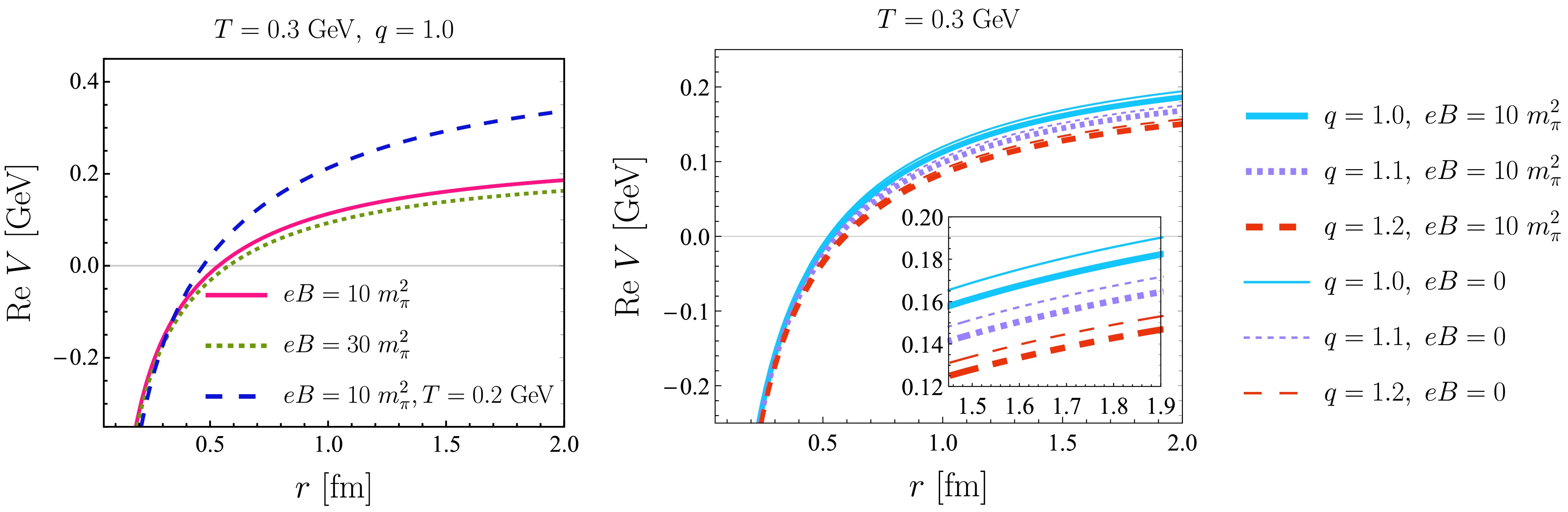
Figure 2. (color online) (Left panel) The real part of the heavy-quark potential,
$ \mathrm{Re}\,V $ , as a function of the quark-antiquark separation r for$ eB=10\; m_{\pi}^2 $ and$ eB=30\; m_{\pi}^2 $ at$ T=0.3 $ GeV with$ q=1.0 $ . A comparison with the result for$ eB=10\; m_{\pi}^2 $ at$ T=0.2 $ GeV is also shown. (Right panel) The r dependence of$ \mathrm{Re}V $ for various values of the non-extensive parameter q at$ T=0.3 $ GeV. In addition, the results at$ eB = 10\; m_{\pi}^2 $ are compared with those at$ eB = 0 $ from Ref. [89]. All the above numerical results are obtained at zero chemical potential. -
Following the approach proposed in [93], the heavy-quark potential in the non-extensive QGP can be determined through the convolution of the Cornell potential with the non-extensively modified dielectric permittivity.
$ V({\rho}) = V_{\rm{Cornell}} ({\rho} ) \varepsilon^{-1}({\rho} ), $
(62) where the Fourier transform of the Cornell potential in momentum space,
$ V_{\rm{Cornell}} ({\rho}) $ , is given by [93]$ V_{\rm{Cornell}} (\rho)=-\sqrt{(2/\pi)} \frac{C_{F}\alpha_{s}}{\rho^2}-\frac{4\sigma}{\sqrt{2 \pi}\rho^4}. $
(63) By performing a Fourier transform, Eq. (62) is cast into real coordinate space and takes the form
$ V({{r}})=\int \frac{{\mathrm{d}}^3 {{\rho}}}{{(2\pi)}^{3/2}} ({\mathrm{e}}^{{\mathrm{i}}{{\rho}} \cdot {{r}}}-1)V_{\rm{Cornell}} (\rho)\varepsilon^{-1}({\rho}). $
(64) Without loss of generality, we choose
$ {{\rho}} $ and$ {{r}} $ as$ {{\rho}}=\rho(\sin\theta\cos\phi,\sin \theta\sin\phi,\cos\theta) $ and$ {{r}}=r(\sin\Phi, 0, \cos\Phi) $ , respectively. Here, Φ denotes the angle between the heavy quark-antiquark dipole axis and the direction of the magnetic field. The dot product$ {{\rho}}\cdot{{r}} $ is given by$ \rho r(\sin\Phi\cos\phi\sin\theta+\cos\Phi\cos\theta) $ . Consequently, Eq. (64) can be rewritten as$ \begin{aligned}[b] V(r,\Phi,q,T,eB)=\;& \int \frac{ \rho^2 \sin\theta {\mathrm{d}}\theta {\mathrm{d}}\rho }{(2\pi)^{1/2}} V_{\rm{Cornell}} (\rho ) \varepsilon^{-1}(\rho )\\ &\times\left[J_{0}(\rho r\sin\theta\sin\Phi){\mathrm{e}}^{{\mathrm{i}}\rho r\cos\theta\cos\Phi}-1\right], \end{aligned} $
(65) where
$ J_{m}(x) $ denotes the Bessel function of the first kind of order m.In this study, the string tension is set to
$ \sigma=0.18\; \mathrm{GeV}^2 $ [95]. The running strong coupling constant g is taken from Ref. [96].$ \alpha_s(\Lambda^2,eB)=\frac{g^2}{4\pi}=\frac{\alpha_s(\Lambda^2)}{1+\dfrac{11N_c-2N_f}{12\pi}\alpha_s(\Lambda^2)\ln \left(\dfrac{\Lambda^2}{\Lambda^2+eB}\right)}, $
(66) where the one-loop QCD strong coupling constant
$ \alpha_s $ at$ eB=0 $ is given by$ \alpha_s(\Lambda^2)=\dfrac{12\pi}{(11N_c-2N_f)\ln\left(\Lambda^2/\Lambda_{\bar{MS}}^2\right)} $ with$ \Lambda_{\bar{MS}}=176\; \mathrm{MeV} $ and$ N_f=N_c=3 $ [97]. The scale Λ is taken to be$ 2\pi\sqrt{T^2+\mu^2/\pi^2} $ for quarks and$ 2\pi T $ for gluons.By inserting the real part of Eq. (61) into Eq. (65), we compute the real part of the heavy-quark potential, denoted by
$ \mathrm{Re}V $ , in the presence of a magnetic field. To order$ (q-1)^0 $ , it can be written as$ \begin{aligned}[b] \mathrm{Re} \,V_{(0)}(r,T, eB) =\;& -C_F\alpha_s \, {m}_{D,B} \left(\frac{{\mathrm{e}}^{-{m}_{D,B}\, r}}{{m}_{D,B}\, r}+1\right) \\ &+ \frac{2\sigma}{{m}_{D,B} }\left(\frac{{\mathrm{e}}^{-{m}_{D,B}\,{r}}-1}{{m}_{D,B}\,r}+1\right). \end{aligned} $
(67) The first and second terms on the right-hand side of Eq. (67) correspond to the HTL and string-like parts of the potential, respectively. To order
$ (q-1)^1 $ , the non-extensive correction to$ \mathrm{Re}\,V $ is given by$ \begin{aligned}[b]&\mathrm{Re}\, V_{(1)}(r,q, T,eB) \\=\;&C_F\alpha_s\frac{m_{D,R,B,(1)}^2}{2m_{D,B} }\left( {\mathrm{e}}^{-m_{D,B} r}-1\right)\\&+\frac{\sigma m_{D,R,B,(1)}^2}{m_{D,B}^3}\left(\frac{2-(2+m_{D,B}r){\mathrm{e}}^{-m_{D,B}r}}{m_{D,B} r}-1\right).\end{aligned} $
(68) In all numerical calculations, the maximum Landau level is set to
$ n_{\mathrm{max}}=100 $ . This choice is justified because, as this cutoff is increased further, the numerical results converge and remain quantitatively unchanged. In the left panel of Fig. 2, we display the real part of the heavy-quark potential,$ \mathrm{Re}\,V $ , as a function of the quark-antiquark separation r for$ eB=10\; m_{\pi}^2 $ and$ eB=30\; m_{\pi}^2 $ at$ T=0.3\; $ GeV, and compare it with$ \mathrm{Re}\,V $ for$ eB=10\; m_{\pi}^2 $ at$ T=0.2 $ GeV. As shown in the figure,$ \mathrm{Re}\,V $ increases rapidly at first and then gradually flattens as r grows. The magnetic field influences$ \mathrm{Re}\,V $ by modifying the quark contributions to the Debye mass and the QCD coupling constant. As the magnetic field and temperature increase, the screening effect strengthens, causing$ \mathrm{Re}\,V $ to become flatter. The right panel of Fig. 2 shows$ \mathrm{Re}\,V $ as a function of r for different values of the non-extensive parameter q at$ T=0.3 $ GeV and$ eB=10\; m_{\pi}^2 $ , compared with the results at vanishing magnetic field ($ eB=0 $ ) [89]. The non-extensive correction alters$ \mathrm{Re}\, V $ by modifying the Debye masses, transforming$ m_{D,B} $ into$ \widetilde{m}_{D, R,B} $ , which leads to a shorter Debye screening length (or equivalently, a larger Debye screening mass). As a result,$ \mathrm{Re}\,V_{} $ flattens with increasing q in a finite magnetic field. We also observe that the magnetic field does not change the qualitative q-dependence of$ \mathrm{Re}\,V $ but further flattens its r-dependence compared with the$ eB=0 $ case. In addition, recent studies have investigated the bulk-viscous correction to the heavy-quark potential in both zero [98, 99] and finite [34] magnetic fields. Notably, Ref. [34] shows that the positive bulk-viscous effect on$ \mathrm{Re}\,V $ is opposite to the non-extensive effect, supporting the statement in Ref. [60] that non-extensivity effectively acts as a negative bulk viscosity.
Figure 2. (color online) (Left panel) The real part of the heavy-quark potential,
$ \mathrm{Re}\,V $ , as a function of the quark-antiquark separation r for$ eB=10\; m_{\pi}^2 $ and$ eB=30\; m_{\pi}^2 $ at$ T=0.3 $ GeV with$ q=1.0 $ . A comparison with the result for$ eB=10\; m_{\pi}^2 $ at$ T=0.2 $ GeV is also shown. (Right panel) The r dependence of$ \mathrm{Re}V $ for various values of the non-extensive parameter q at$ T=0.3 $ GeV. In addition, the results at$ eB = 10\; m_{\pi}^2 $ are compared with those at$ eB = 0 $ from Ref. [89]. All the above numerical results are obtained at zero chemical potential. -
Next, we study the imaginary part of the in-medium heavy-quark potential, denoted by
$ \mathrm{Im}\,V $ , which is related to inelastic scattering between medium constituents and heavy quarkonium via the exchange of space-like gluons (the Landau damping phenomenon) within HTL-resummed perturbation theory [100]. The gluonic and quark contributions to the gluon self-energy, particularly in a finite magnetic field, differ strikingly in form. Therefore, we analyze their contributions to$ \mathrm{Im}\,V $ separately to elucidate the qualitative features of the potential. First, we examine the imaginary part of the potential associated with the gluonic contribution to the gluon self-energy,$ \mathrm{Im}\,V^{\rm{gluon}} $ . By inserting the first term of Eq. (57) into Eq. (65), we compute$ \mathrm{Im}V^{\rm{gluon}} $ to order$ (q-1)^0 $ as$ \begin{aligned}[b] \mathrm{Im}\,V_{(0)}^{\rm{gluon}}(r,T,eB) =\;& -C_F\alpha_sT\frac{({m}_{D}^{\rm{gluon}})^2 }{{m}_{D,B}^2}\phi_2({m}_{D,B}r)\\ & -\frac{2\sigma T ({m}_{D}^{\rm{gluon}})^2}{{m}_{D,B}^4}\chi_2({m}_{D,B} r) . \end{aligned} $
(69) By substituting Eq. (58) into Eq. (65), the
$ \mathrm{Im}\,V^{\rm{gluon}} $ to order$ (q-1)^1 $ is given by$ \begin{aligned}[b] \mathrm{Im}\,V_{(1)}^{\rm{gluon}}(r,q,T, eB) =\;& -\frac{T({m}_{D,F,(1)}^{\rm{gluon}})^2 }{{m}_{D,B}^2}\left[C_F\alpha_s\phi_2({m}_{D,B}r)+\frac{2\sigma}{{m}_{D,B}^2}\chi_2({m}_{D,B} r)\right]\\& +\frac{2T(m_{D,R,(1)}^{\rm{gluon}})^2(m_{D}^{\rm{gluon}})^2}{m_{D,B}^4}\left[C_F\alpha_s \phi_{3}(m_{D,B}r)+\frac{2\sigma}{m_{D,B}^2}\chi_3(m_{D,B}r)\right]\\&-\frac{4T}{\pi}(m_{D,R,(1)}^{\rm{gluon}})^2\int\rho^2 \sin\theta {\mathrm{d}}\theta {\mathrm{d}}\rho\frac{J_{0}(\rho r\sin\theta\sin\Phi){\mathrm{e}}^{{\mathrm{i}}\rho r\cos\theta\cos\Phi}-1}{({\rho}^2+{m}_{D,B}^2)^3}\left(C_F\alpha_s+\frac{2\sigma}{\rho^2}\right)\\ & \times\left[\sum\limits_{f} \alpha_s|e_fB|)\delta(\rho\cos\theta)+ \sum\limits_{f}\sum\limits_{n=1}^{\infty}\sum\limits_{b=\pm}\frac{\alpha_s 2n|e_fB|^2H_b^f(E_{\rho_z/2,n}^f)}{ T|\rho_z|E^f_{\rho_z/2,n}}\right]. \end{aligned} $
(70) The functions
$ \phi_n(x) $ and$ \chi_n(x) $ are defined by$ \phi_n (x) \equiv 2 \int_{0}^{\infty} dz \dfrac{z}{(z^{2}+1)^{n}}\left[1-\dfrac{\sin(x z)}{x z}\right] $ , and$ \chi_n (x) \equiv 2 \int_{0}^{\infty} \dfrac{{\mathrm{d}}z}{z(z^{2}+1)^{n}} \left[1-\dfrac{\sin(x z)}{x z}\right] $ , respectively. Although the last term of Eq. (70) exhibits angular dependence, its magnitude is negligible compared with the other terms, allowing$ \mathrm{Im}\,V^{\rm{gluon}}_{1} $ to be reasonably approximated as isotropic.In the left panel of Fig. 3, we plot the dependence of
$ \mathrm{Im} V^{\rm{gluon}} $ on the quark-antiquark separation distance r for$ eB=10\; m_{\pi}^2 $ and$ eB=30\; m_{\pi}^2 $ at$ T=0.3\; $ GeV, and compare it with the result for$ eB=10\; m_{\pi}^2 $ at$ T=0.2 $ GeV. We see that$ \mathrm{Im}\,V^{\rm{gluon}} $ decreases with increasing r. In contrast to the real part of the potential, the magnetic field and temperature can increase$ \mathrm{Im} V^{\rm{gluon}} $ . In the right panel of Fig. 3, we show$ \mathrm{Im} V^{\rm{gluon}} $ for different values of the non-extensive parameter q at$ eB=10\; m_{\pi}^2 $ and$ T=0.3\; $ GeV. It is clear that the magnitude of$ \mathrm{Im}\,V^{\rm{gluon}} $ exhibits an increasing trend with q.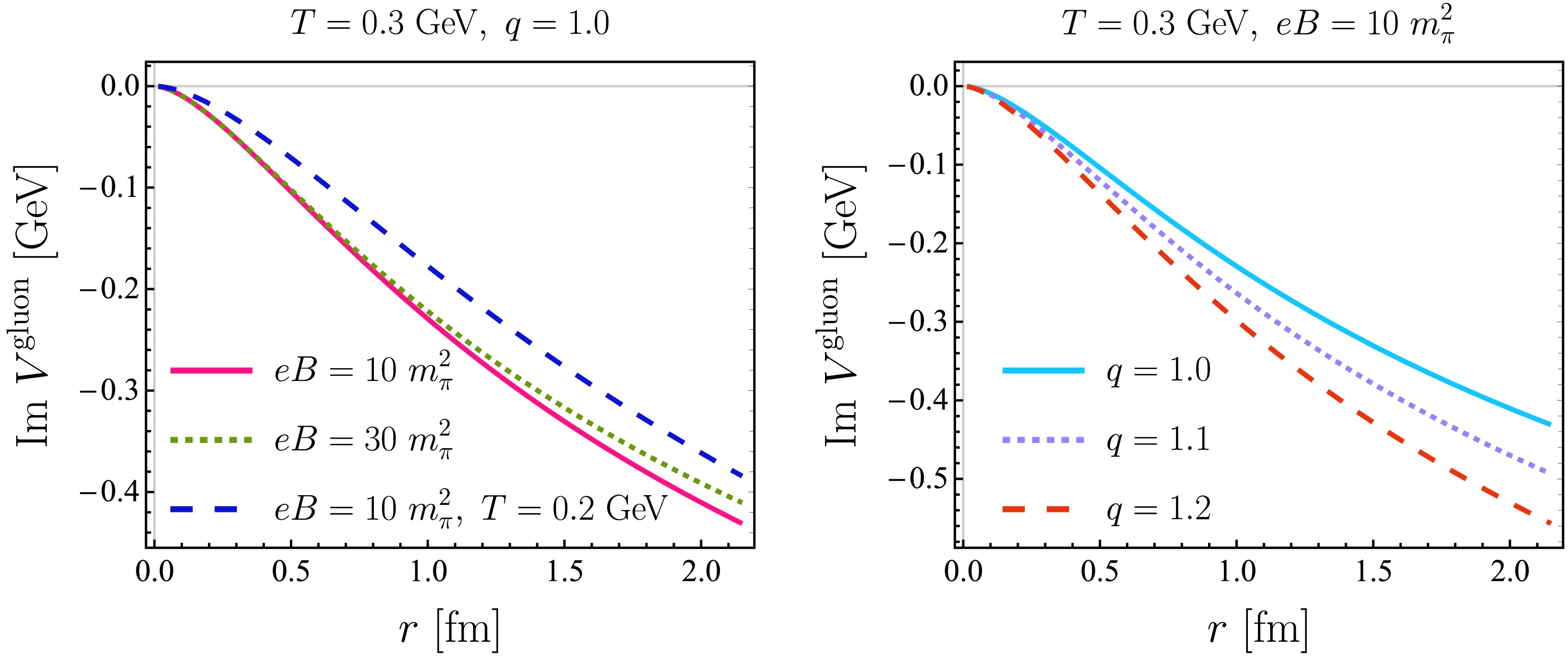
Figure 3. (color online) (Left panel) The imaginary part of the heavy-quark potential arising from the one-loop gluon contribution to the gluon self-energy,
$ \mathrm{Im}\,V^{\rm{gluon}} $ , as a function of the quark-antiquark separation distance r for$ eB=10\; m_{\pi}^2 $ and$ eB=30\; m_{\pi}^2 $ at$ T=0.3 $ GeV with$ q=1.0 $ . This panel also includes a comparison with the result for$ eB=10\; m_{\pi}^2 $ at$ T=0.2 $ GeV. (Right panel) The r-dependence of$ \mathrm{Im}\,V^{\rm{gluon}} $ for various values of the non-extensive parameter q at$ T=0.3 $ GeV and$ eB=10\; m_{\pi}^2 $ .Next, we study the imaginary part of the potential associated with the quark contribution to the gluon self-energy,
$ \mathrm{Im}\,V^{\rm{quark}} $ . By inserting the second term of Eq. (57) into Eq. (65),$ \mathrm{Im}V^{\rm{quark}} $ to order$ (q-1)^0 $ is obtained as follows:$ \begin{aligned}[b]\mathrm{Im}\,V_{(0)}^{\rm{quark}}(r,\Phi,T,eB) =\;& \int\rho^2 \sin\theta {\mathrm{d}}\theta {\mathrm{d}}\rho\left[J_{0}(\rho r\sin\theta\sin\Phi){\mathrm{e}}^{{\mathrm{i}}\rho r\cos\theta\cos\Phi}-1\right]\\& \times\left[ \sum\limits_{f}\sum\limits_{n=1}^{\infty}\sum\limits_{b=\pm}\frac{ \alpha_s4n|e_fB|^2H^f_{b}(E_{\rho_z/2,n}^f)}{({\rho}^2+m_{D,B}^2)^2|\rho_z|E^f_{\rho_z/2,n}}\right]\left(\frac{C_F\alpha_s }{\pi}+\frac{2\sigma}{\rho^2\pi}\right). \end{aligned}$
(71) Here,
$ E_{\rho_z/2,n}^f $ can be rewritten as$ E_{\rho_z/2,n}^f=\sqrt{(\rho\cos\theta/2)^2+2n|e_fB|} $ . By substituting Eq. (59) into Eq. (65), we derive the non-extensive correction term for$ \mathrm{Im}V^{\rm{quark}} $ , up to order$ (q-1)^1 $ , which is given by$ \begin{aligned}[b]\mathrm{Im}\,V_{(1)}^{\rm{quark}}(r,\Phi, q,T,eB) =\;& {\frac{2\big(m_{D,R,B(1)}^{\rm{quark}}\big)^2\big(m_{D}^{\rm{gluon}}\big)^2}{m_{D,B}^4}\left[TC_F\alpha_s \phi_{3}(m_{D,B}r)+T\frac{2\sigma}{m_{D,B}^2}\chi_3(m_{D,B}r)\right]}\\& {-\frac{4T}{\pi}(m_{D,R,B(1)}^{\rm{quark}})^2\int\rho^2 \sin\theta {\mathrm{d}}\theta {\mathrm{d}}\rho\frac{\left[J_{0}(\rho r\sin\theta\sin\Phi){\mathrm{e}}^{{\mathrm{i}}\rho r\cos\theta\cos\Phi}-1\right]}{({\rho}^2+{m}_{D,B}^2)^3}\left(C_F\alpha_s+\frac{2\sigma}{\rho^2}\right)}\\& {\times\left[\sum\limits_{f}\alpha_s|e_fB|)\delta(\rho\cos\theta)+ \sum\limits_{f}\sum\limits_{n=1}^{\infty}\sum\limits_{b=\pm}\frac{ \alpha_s 2n|e_fB|^2H_b^f(E_{\rho_z/2,n}^f)}{ T|\rho_z|E^f_{\rho_z/2,n}}\right]}\\&{+\frac{1}{2\pi}\int \rho^2 \sin\theta {\mathrm{d}}\theta {\mathrm{d}}\rho\frac{J_{0}(\rho r\sin\theta\sin\Phi){\mathrm{e}}^{{\mathrm{i}}\rho r\cos\theta\cos\Phi}-1}{(\rho^2+{m}_{D,B}^2)^2}\left(C_F\alpha_s+\frac{2\sigma}{\rho^2}\right)}\\& {\times\left[\sum\limits_{f}\sum\limits_{n=1}^{\infty}\sum\limits_{b=\pm}\frac{\alpha_s 8n|e_fB|^2 }{E_{\rho_z/2,n}^f|\rho_z|}\frac{q-1}{2}W^f_{b} (E_{\rho_z/2,n}^f)\right]}. \end{aligned} $
(72) In Fig. 4, we plot the imaginary part of the heavy quark potential associated with the quark contribution to the gluon self-energy,
$ \mathrm{Im}\,V^{\rm{quark}} $ , as a function of separation distance for different values of angle between the quark-antiquark dipole axis and the direction of a magnetic field at$ eB=10\; m_{\pi}^2 $ and$ T=0.3\; $ GeV. We observe that$ \mathrm{Im}\,V^{\rm{quark}} $ exhibits a significant anisotropy in the presence of a magnetic field. Specifically, the magnitude of$ \mathrm{Im}\,V^{\rm{quark}} $ exhibits a maximum at$ \Phi=\pi/2 $ , at which the quark-antiquark dipole axis is perpendicular to the direction of the magnetic field. Conversely, a minimum of the magnitude of$ \mathrm{Im}\,V^{\rm{quark}} $ is observed at$ \Phi=0 $ , where the quark-antiquark dipole axis is parallel to the magnetic field direction. As the separation distance increases further, the anisotropy of$ \mathrm{Im}\, V^{\rm{quark}} $ gradually diminishes. This is actually expected, since the correlation of a heavy quark and its antiquark must be independent, in the large distance limit, from the direction of their relative separation. Moreover, the decreasing trend of$ \mathrm{Im}\, V^{\rm{quark}} $ with increasing r remains consistent, regardless of the variation in Φ.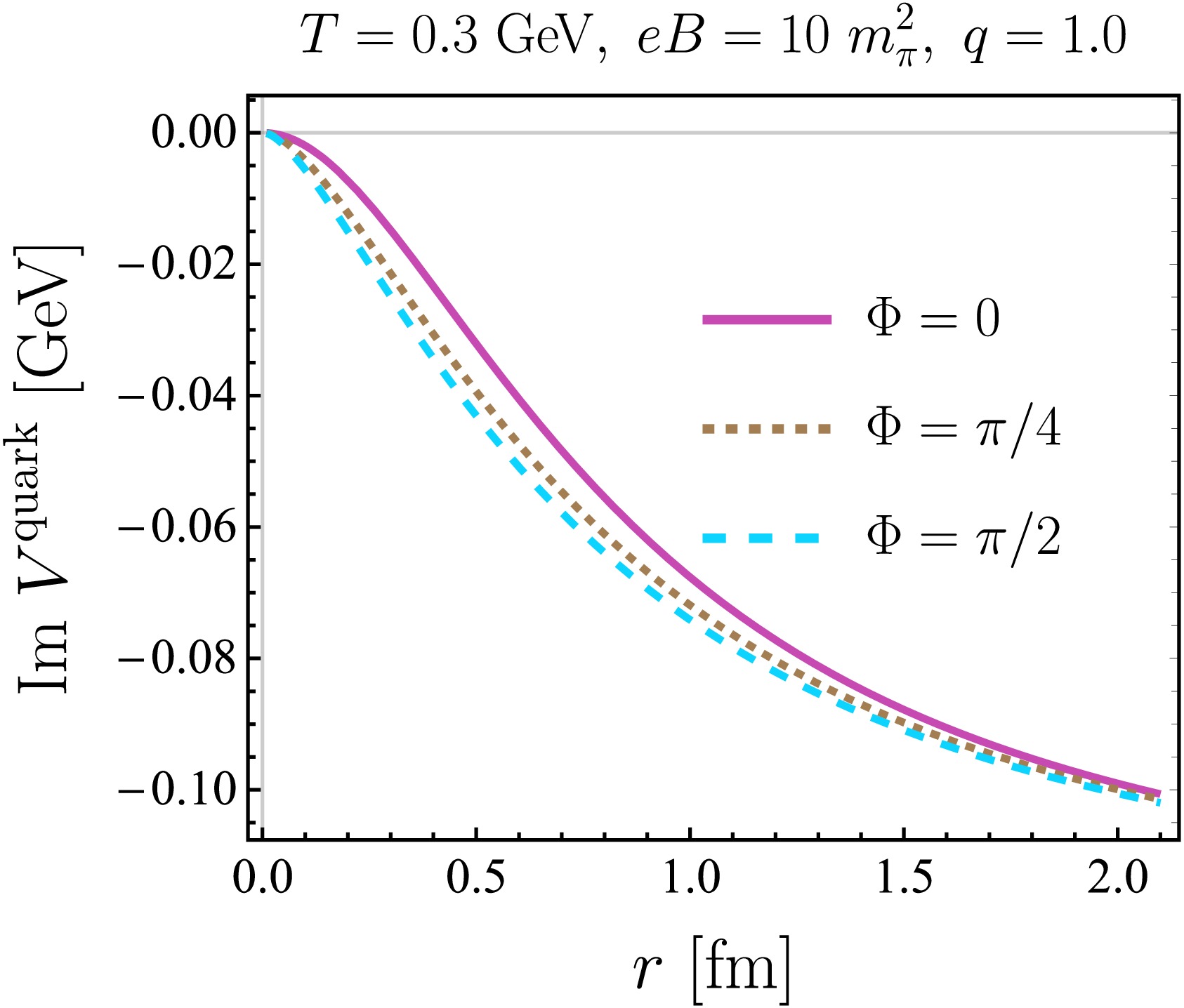
Figure 4. (color online) The imaginary part of the heavy-quark potential arising from the one-loop quark contributions to the gluon self-energy,
$ \mathrm{Im}\,V^{\rm quark} $ , is shown as a function of the quark-antiquark separation r for$ q=1.0 $ . The plot presents results for different values of the angle Φ between the quark-antiquark dipole axis and the magnetic-field direction (i.e.,$ \Phi=0 $ ,$ \pi/4 $ , and$ \pi/2 $ ).} at$ eB=10 m_{\pi}^2 $ and$ T=0.3 $ GeV.In the left panel of Fig. 5, we present the r-dependence of
$ \mathrm{Im} V^{\rm{quark}} $ for$ eB=10\; m_{\pi}^2 $ and for$ eB=30\; m_{\pi}^2 $ at$ T=0.3\; $ GeV, which is compared to the result for$ eB=10\; m_{\pi}^2 $ at$ T=0.2 $ GeV. We observe that as q increases$ \mathrm{Im}\,V^{\rm{quark}} $ gradually decreases. Whereas, the increase of magnetic field and temperature leads to an enhancement of$ \mathrm{Im} V^{\rm{quark}} $ . In the right panel of Fig. 5, we show the behavior of$ \mathrm{Im} \,V^{\rm{quark}} $ with respect to different values of non-extensive parameter q at$ eB=10\; m_{\pi}^2 $ and$ T=0.3\; $ GeV in the case of$ \Phi=0 $ . Similar to$ \mathrm{Im}\,V^{\rm{gluon}} $ , the magnitude of$ \mathrm{Im} \,V^{\rm{quark}} $ also increases as q increases. The decreasing feature of both$ \mathrm{Im}\,V^{\rm{gluon}} $ and$ \mathrm{Im}\,V^{\rm{quark}} $ with q and r, is naturally reflected in the total imaginary part of the potential$ \mathrm{Im}\,V^{{\rm{gluon}}}=\mathrm{Im}V^{\rm{gluon}}+\mathrm{Im}V^{\rm{quark}} $ , as shown in Fig. 6. We also display the r-dependence of$ \mathrm{Im}\,V $ for different q at zero and finite magnetic fields. We observe that the presence of a magnetic field marginally affects the q-dependence of$ \mathrm{Im}\,V $ but significantly reduces the magnitude of$ \mathrm{Im}\,V $ compared to the$ eB=0 $ case. The bulk viscous correction to the imaginary part of the potential has also been studied in [99], within the same potential description as ours. In contrast to our finding that non-extensive effects ($ q>1 $ ) suppress$ \mathrm{Im}\,V $ , Ref. [99] reported that the positive bulk viscosity (or negative bulk pressure) leads to an enhancement of$ \mathrm{Im}\,V $ .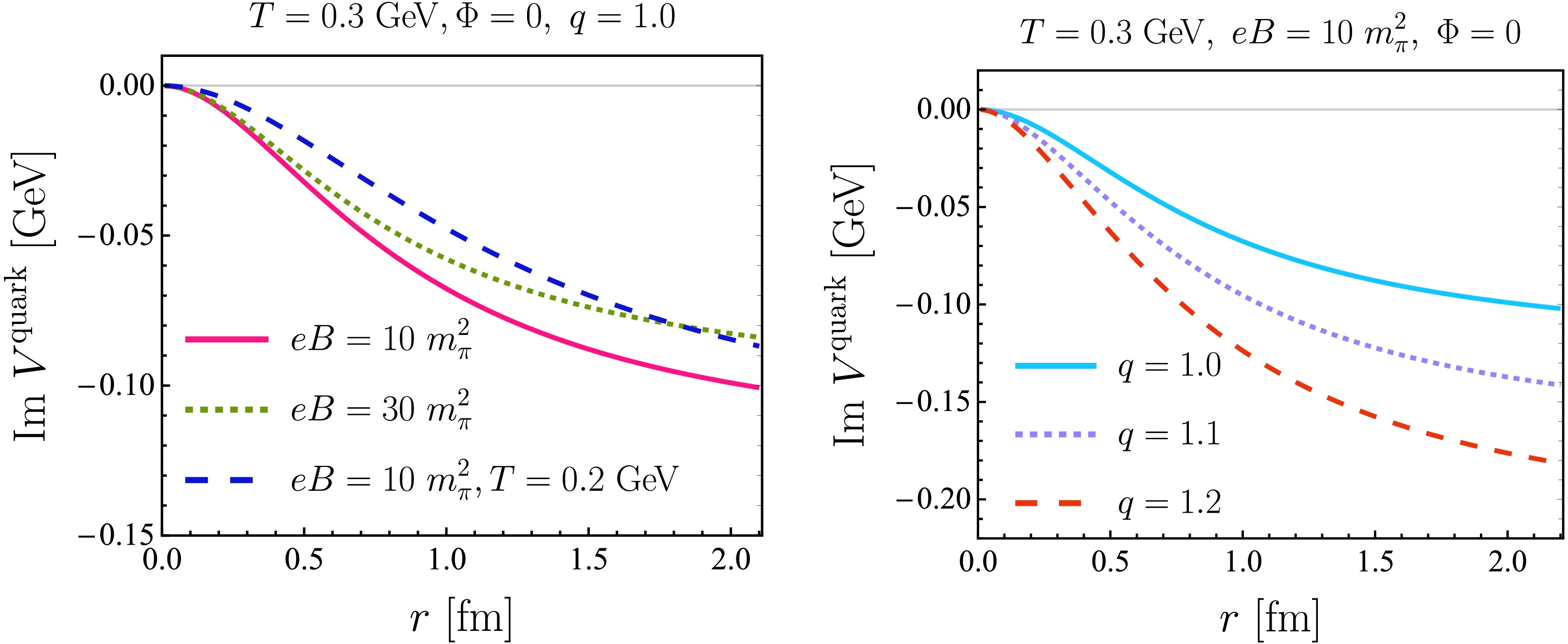
Figure 5. (color online) Same as Fig. 3, but for
$ \mathrm{Im}\,V^{\rm{quark}} $ , with the quark-antiquark dipole axis parallel to the magnetic field direction ($ \Phi = 0 $ ).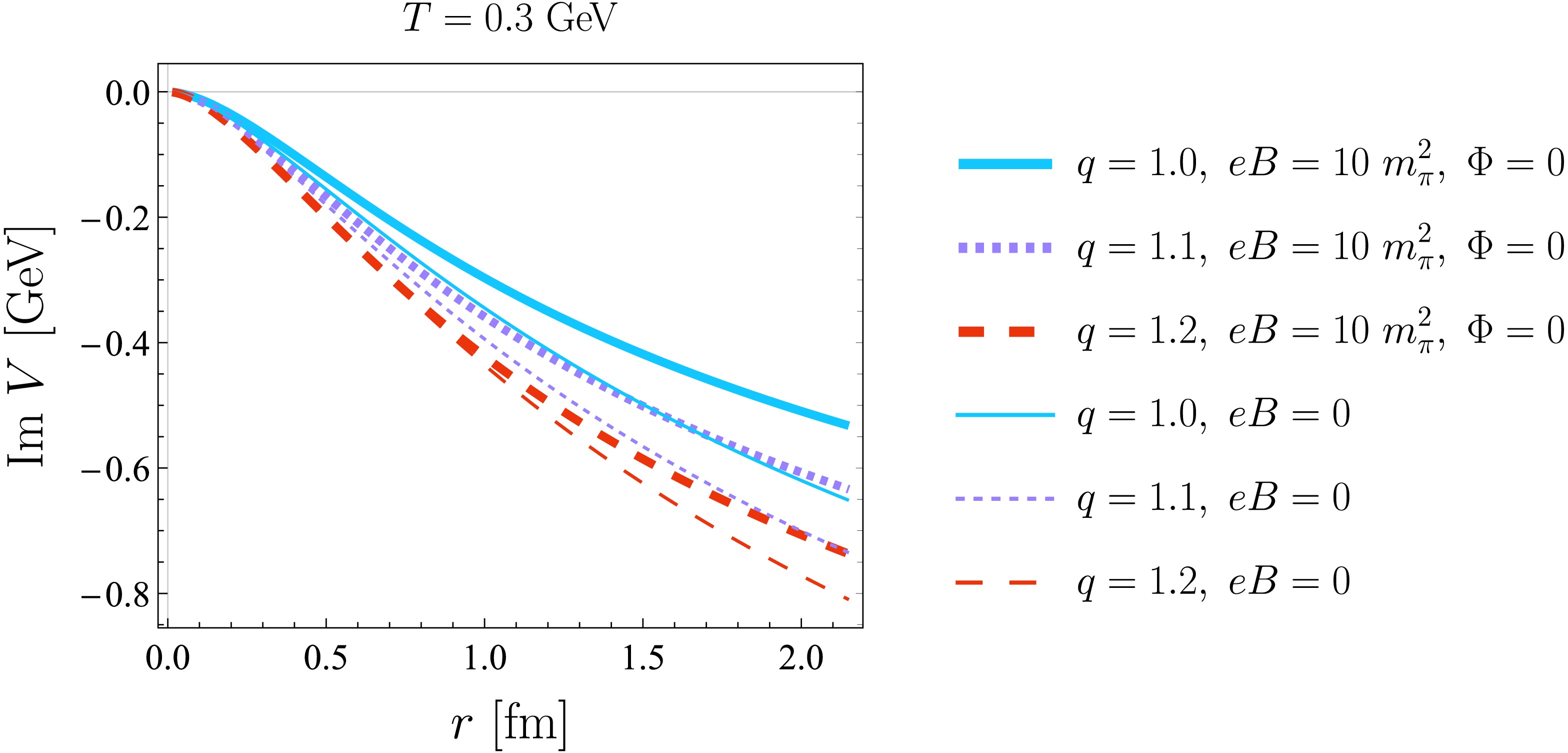
Figure 6. (color online) The r-dependence of the total imaginary part of the heavy-quark potential,
$ \mathrm{Im}\,V=\mathrm{Im}\,V^{\rm{gluon}}+\mathrm{Im}\,V^{\rm{quark}} $ , is shown for different values of q at$ eB=10\; m_{\pi}^2 $ . The quark-antiquark dipole axis is parallel to the magnetic-field direction (i.e.,$ \Phi=0 $ ). For comparison, the corresponding results at$ eB=0 $ from Ref. [89] are also shown. All numerical calculations are performed at$ T=0.3 $ GeV and zero chemical potential.To clarify the anisotropic response of the imaginary part of the potential in finite magnetic field to non-extensivity, in Fig. 7, we plot two anisotropy ratios as a function of non-extensive parameter q at
$ eB=10\; m_{\pi}^2 $ and$ T=0.3\; $ GeV. The first is the anisotropy ratio of$ \mathrm{Im}\, V^{\rm{quark}} $ , defined as$ \bar{R}=\frac{\mathrm{Im}\,V^{\rm{quark}}(\Phi=0)}{\mathrm{Im}\,V^{\rm{quark}}(\Phi=\pi/2)} $ . The second is the anisotropy ratio of$ \mathrm{Im}\, V $ , defined as$ R=\frac{\mathrm{Im}\,V(\Phi=0)}{\mathrm{Im}\,V(\Phi=\pi/2)} $ . The left panel of Fig. 7 shows the results for$ r=0.5\; $ fm, while the right panel shows the results for$ r=1\; $ fm. We observe that at the small separation distance ($ 0.5 $ fm), the degree of anisotropy in the imaginary part of the potential is higher than that at the large separation distance ($ r=1\; $ fm). We also note that varying the values of q significantly changes the anisotropy ratio of$ \mathrm{Im}\,V^{\rm{quark}} $ quantitatively. Specifically, with increasing q, the anisotropy degree of$ \mathrm{Im}\; V^{\rm{quark}} $ is gradually weakened. After accounting for the contribution from$ \mathrm{Im}V^{\rm{gluon}} $ , the anisotropic feature of$ \mathrm{Im}\,V $ in finite magnetic field becomes minimal, and the anisotropy ratio of$ \mathrm{Im}\,V $ becomes almost insensitive to the variation of non-extensivity.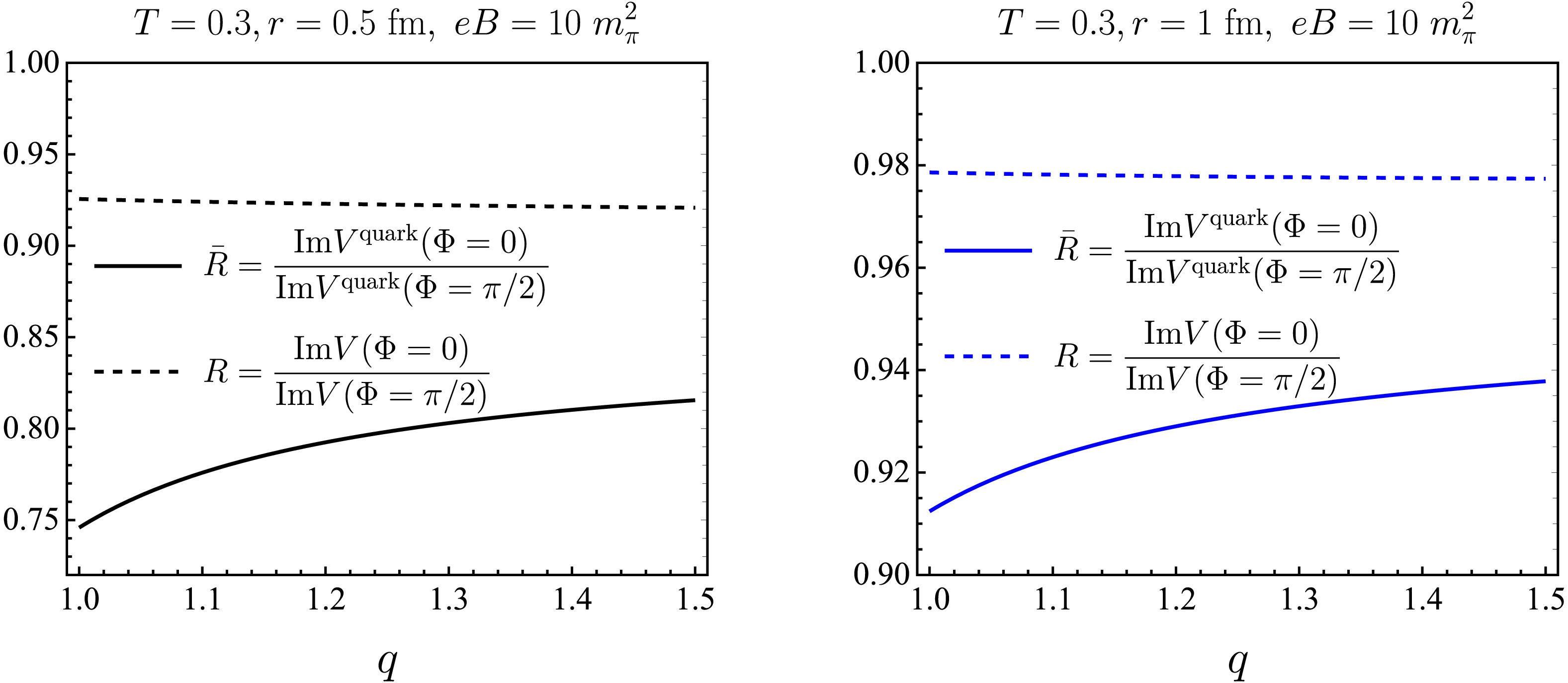
Figure 7. (color online) The anisotropy ratios
$ \bar{R}=\frac{\mathrm{Im}\,V^{\rm{quark}}(\Phi=0)}{\mathrm{Im}\,V^{\rm{quark}}(\Phi=\pi/2)} $ and$ R=\frac{\mathrm{Im}\,V(\Phi=0)}{\mathrm{Im}\,V(\Phi=\pi/2)} $ are shown as functions of the nonextensive parameter q for$ eB=15\; m_{\pi}^2 $ at$ r=0.5 $ fm (left panel) and$ r=1 $ fm (right panel). -
Next, we study the imaginary part of the in-medium heavy-quark potential, denoted by
$ \mathrm{Im}\,V $ , which is related to inelastic scattering between medium constituents and heavy quarkonium via the exchange of space-like gluons (the Landau damping phenomenon) within HTL-resummed perturbation theory [100]. The gluonic and quark contributions to the gluon self-energy, particularly in a finite magnetic field, differ strikingly in form. Therefore, we analyze their contributions to$ \mathrm{Im}\,V $ separately to elucidate the qualitative features of the potential. First, we examine the imaginary part of the potential associated with the gluonic contribution to the gluon self-energy,$ \mathrm{Im}\,V^{\rm{gluon}} $ . By inserting the first term of Eq. (57) into Eq. (65), we compute$ \mathrm{Im}V^{\rm{gluon}} $ to order$ (q-1)^0 $ as$ \begin{aligned}[b] \mathrm{Im}\,V_{(0)}^{\rm{gluon}}(r,T,eB) =\;& -C_F\alpha_sT\frac{({m}_{D}^{\rm{gluon}})^2 }{{m}_{D,B}^2}\phi_2({m}_{D,B}r)\\ & -\frac{2\sigma T ({m}_{D}^{\rm{gluon}})^2}{{m}_{D,B}^4}\chi_2({m}_{D,B} r) . \end{aligned} $
(69) By substituting Eq. (58) into Eq. (65), the
$ \mathrm{Im}\,V^{\rm{gluon}} $ to order$ (q-1)^1 $ is given by$ \begin{aligned}[b] \mathrm{Im}\,V_{(1)}^{\rm{gluon}}(r,q,T, eB) =\;& -\frac{T({m}_{D,F,(1)}^{\rm{gluon}})^2 }{{m}_{D,B}^2}\left[C_F\alpha_s\phi_2({m}_{D,B}r)+\frac{2\sigma}{{m}_{D,B}^2}\chi_2({m}_{D,B} r)\right]\\& +\frac{2T(m_{D,R,(1)}^{\rm{gluon}})^2(m_{D}^{\rm{gluon}})^2}{m_{D,B}^4}\left[C_F\alpha_s \phi_{3}(m_{D,B}r)+\frac{2\sigma}{m_{D,B}^2}\chi_3(m_{D,B}r)\right]\\&-\frac{4T}{\pi}(m_{D,R,(1)}^{\rm{gluon}})^2\int\rho^2 \sin\theta d\theta d\rho\frac{J_{0}(\rho r\sin\theta\sin\Phi)e^{i\rho r\cos\theta\cos\Phi}-1}{({\rho}^2+{m}_{D,B}^2)^3}\left(C_F\alpha_s+\frac{2\sigma}{\rho^2}\right)\\ & \times\left[\sum\limits_{f} \alpha_s|e_fB|)\delta(\rho\cos\theta)+ \sum\limits_{f}\sum\limits_{n=1}^{\infty}\sum\limits_{b=\pm}\frac{\alpha_s 2n|e_fB|^2H_b^f(E_{\rho_z/2,n}^f)}{ T|\rho_z|E^f_{\rho_z/2,n}}\right]. \end{aligned} $
(70) The functions
$ \phi_n(x) $ and$ \chi_n(x) $ are defined by$ \phi_n (x) \equiv 2 \int_{0}^{\infty} dz \dfrac{z}{(z^{2}+1)^{n}}\left[1-\dfrac{\sin(x z)}{x z}\right] $ , and$ \chi_n (x) \equiv 2 \int_{0}^{\infty} \dfrac{dz}{z(z^{2}+1)^{n}} \left[1-\dfrac{\sin(x z)}{x z}\right] $ , respectively. Although the last term of Eq. (70) exhibits angular dependence, its magnitude is negligible compared with the other terms, allowing$ \mathrm{Im}\,V^{\rm{gluon}}_{1} $ to be reasonably approximated as isotropic.In the left panel of Fig. 3, we plot the dependence of
$ \mathrm{Im} V^{\rm{gluon}} $ on the quark-antiquark separation distance r for$ eB=10\; m_{\pi}^2 $ and$ eB=30\; m_{\pi}^2 $ at$ T=0.3\; $ GeV, and compare it with the result for$ eB=10\; m_{\pi}^2 $ at$ T=0.2 $ GeV. We see that$ \mathrm{Im}\,V^{\rm{gluon}} $ decreases with increasing r. In contrast to the real part of the potential, the magnetic field and temperature can increase$ \mathrm{Im} V^{\rm{gluon}} $ . In the right panel of Fig. 3, we show$ \mathrm{Im} V^{\rm{gluon}} $ for different values of the non-extensive parameter q at$ eB=10\; m_{\pi}^2 $ and$ T=0.3\; $ GeV. It is clear that the magnitude of$ \mathrm{Im}\,V^{\rm{gluon}} $ exhibits an increasing trend with q.
Figure 3. (color online) (Left panel) The imaginary part of the heavy-quark potential arising from the one-loop gluon contribution to the gluon self-energy,
$ \mathrm{Im}\,V^{\rm{gluon}} $ , as a function of the quark-antiquark separation distance r for$ eB=10\; m_{\pi}^2 $ and$ eB=30\; m_{\pi}^2 $ at$ T=0.3 $ GeV with$ q=1.0 $ . This panel also includes a comparison with the result for$ eB=10\; m_{\pi}^2 $ at$ T=0.2 $ GeV. (Right panel) The r-dependence of$ \mathrm{Im}\,V^{\rm{gluon}} $ for various values of the non-extensive parameter q at$ T=0.3 $ GeV and$ eB=10\; m_{\pi}^2 $ .Next, we study the imaginary part of the potential associated with the quark contribution to the gluon self-energy,
$ \mathrm{Im}\,V^{\rm{quark}} $ . By inserting the second term of Eq. (57) into Eq. (65),$ \mathrm{Im}V^{\rm{quark}} $ to order$ (q-1)^0 $ is obtained as follows:$ \begin{aligned}[b]\mathrm{Im}\,V_{(0)}^{\rm{quark}}(r,\Phi,T,eB) =\;& \int\rho^2 \sin\theta d\theta d\rho\left[J_{0}(\rho r\sin\theta\sin\Phi)e^{i\rho r\cos\theta\cos\Phi}-1\right]\\& \times\left[ \sum\limits_{f}\sum\limits_{n=1}^{\infty}\sum\limits_{b=\pm}\frac{ \alpha_s4n|e_fB|^2H^f_{b}(E_{\rho_z/2,n}^f)}{({\rho}^2+m_{D,B}^2)^2|\rho_z|E^f_{\rho_z/2,n}}\right]\left(\frac{C_F\alpha_s }{\pi}+\frac{2\sigma}{\rho^2\pi}\right). \end{aligned}$
(71) Here,
$ E_{\rho_z/2,n}^f $ can be rewritten as$ E_{\rho_z/2,n}^f=\sqrt{(\rho\cos\theta/2)^2+2n|e_fB|} $ . By substituting Eq. (59) into Eq. (65), we derive the non-extensive correction term for$ \mathrm{Im}V^{\rm{quark}} $ , up to order$ (q-1)^1 $ , which is given by$ \begin{aligned}[b]\mathrm{Im}\,V_{(1)}^{\rm{quark}}(r,\Phi, q,T,eB) =\;& {\frac{2\big(m_{D,R,B(1)}^{\rm{quark}}\big)^2\big(m_{D}^{\rm{gluon}}\big)^2}{m_{D,B}^4}\left[TC_F\alpha_s \phi_{3}(m_{D,B}r)+T\frac{2\sigma}{m_{D,B}^2}\chi_3(m_{D,B}r)\right]}\\& {-\frac{4T}{\pi}(m_{D,R,B(1)}^{\rm{quark}})^2\int\rho^2 \sin\theta d\theta d\rho\frac{\left[J_{0}(\rho r\sin\theta\sin\Phi)e^{i\rho r\cos\theta\cos\Phi}-1\right]}{({\rho}^2+{m}_{D,B}^2)^3}\left(C_F\alpha_s+\frac{2\sigma}{\rho^2}\right)}\\& {\times\left[\sum\limits_{f}\alpha_s|e_fB|)\delta(\rho\cos\theta)+ \sum\limits_{f}\sum\limits_{n=1}^{\infty}\sum\limits_{b=\pm}\frac{ \alpha_s 2n|e_fB|^2H_b^f(E_{\rho_z/2,n}^f)}{ T|\rho_z|E^f_{\rho_z/2,n}}\right]}\\&{+\frac{1}{2\pi}\int \rho^2 \sin\theta d\theta d\rho\frac{J_{0}(\rho r\sin\theta\sin\Phi)e^{i\rho r\cos\theta\cos\Phi}-1}{(\rho^2+{m}_{D,B}^2)^2}\left(C_F\alpha_s+\frac{2\sigma}{\rho^2}\right)}\\& {\times\left[\sum\limits_{f}\sum\limits_{n=1}^{\infty}\sum\limits_{b=\pm}\frac{\alpha_s 8n|e_fB|^2 }{E_{\rho_z/2,n}^f|\rho_z|}\frac{q-1}{2}W^f_{b} (E_{\rho_z/2,n}^f)\right]}. \end{aligned} $
(72) In Fig. 4, we plot the imaginary part of the heavy quark potential associated with the quark contribution to the gluon self-energy,
$ \mathrm{Im}\,V^{\rm{quark}} $ , as a function of separation distance for different values of angle between the quark-antiquark dipole axis and the direction of a magnetic field at$ eB=10\; m_{\pi}^2 $ and$ T=0.3\; $ GeV. We observe that$ \mathrm{Im}\,V^{\rm{quark}} $ exhibits a significant anisotropy in the presence of a magnetic field. Specifically, the magnitude of$ \mathrm{Im}\,V^{\rm{quark}} $ exhibits a maximum at$ \Phi=\pi/2 $ , at which the quark-antiquark dipole axis is perpendicular to the direction of the magnetic field. Conversely, a minimum of the magnitude of$ \mathrm{Im}\,V^{\rm{quark}} $ is observed at$ \Phi=0 $ , where the quark-antiquark dipole axis is parallel to the magnetic field direction. As the separation distance increases further, the anisotropy of$ \mathrm{Im}\, V^{\rm{quark}} $ gradually diminishes. This is actually expected, since the correlation of a heavy quark and its antiquark must be independent, in the large distance limit, from the direction of their relative separation. Moreover, the decreasing trend of$ \mathrm{Im}\, V^{\rm{quark}} $ with increasing r remains consistent, regardless of the variation in Φ.
Figure 4. (color online) The imaginary part of the heavy-quark potential arising from the one-loop quark contributions to the gluon self-energy,
$ \mathrm{Im}\,V^{\rm quark} $ , is shown as a function of the quark-antiquark separation r for$ q=1.0 $ . The plot presents results for different values of the angle Φ between the quark-antiquark dipole axis and the magnetic-field direction (i.e.,$ \Phi=0 $ ,$ \pi/4 $ , and$ \pi/2 $ ).} at$ eB=10 m_{\pi}^2 $ and$ T=0.3 $ GeV.In the left panel of Fig. 5, we present the r-dependence of
$ \mathrm{Im} V^{\rm{quark}} $ for$ eB=10\; m_{\pi}^2 $ and for$ eB=30\; m_{\pi}^2 $ at$ T=0.3\; $ GeV, which is compared to the result for$ eB=10\; m_{\pi}^2 $ at$ T=0.2 $ GeV. We observe that as q increases$ \mathrm{Im}\,V^{\rm{quark}} $ gradually decreases. Whereas, the increase of magnetic field and temperature leads to an enhancement of$ \mathrm{Im} V^{\rm{quark}} $ . In the right panel of Fig. 5, we show the behavior of$ \mathrm{Im} \,V^{\rm{quark}} $ with respect to different values of non-extensive parameter q at$ eB=10\; m_{\pi}^2 $ and$ T=0.3\; $ GeV in the case of$ \Phi=0 $ . Similar to$ \mathrm{Im}\,V^{\rm{gluon}} $ , the magnitude of$ \mathrm{Im} \,V^{\rm{quark}} $ also increases as q increases. The decreasing feature of both$ \mathrm{Im}\,V^{\rm{gluon}} $ and$ \mathrm{Im}\,V^{\rm{quark}} $ with q and r, is naturally reflected in the total imaginary part of the potential$ \mathrm{Im}\,V^{{\rm{gluon}}}=\mathrm{Im}V^{\rm{gluon}}+\mathrm{Im}V^{\rm{quark}} $ , as shown in Fig. 6. We also display the r-dependence of$ \mathrm{Im}\,V $ for different q at zero and finite magnetic fields. We observe that the presence of a magnetic field marginally affects the q-dependence of$ \mathrm{Im}\,V $ but significantly reduces the magnitude of$ \mathrm{Im}\,V $ compared to the$ eB=0 $ case. The bulk viscous correction to the imaginary part of the potential has also been studied in [99], within the same potential description as ours. In contrast to our finding that non-extensive effects ($ q>1 $ ) suppress$ \mathrm{Im}\,V $ , Ref. [99] reported that the positive bulk viscosity (or negative bulk pressure) leads to an enhancement of$ \mathrm{Im}\,V $ .
Figure 5. (color online) Same as Fig. 3, but for
$ \mathrm{Im}\,V^{\rm{quark}} $ , with the quark-antiquark dipole axis parallel to the magnetic field direction ($ \Phi = 0 $ ).
Figure 6. (color online) The r-dependence of the total imaginary part of the heavy-quark potential,
$ \mathrm{Im}\,V=\mathrm{Im}\,V^{\rm{gluon}}+\mathrm{Im}\,V^{\rm{quark}} $ , is shown for different values of q at$ eB=10\; m_{\pi}^2 $ . The quark-antiquark dipole axis is parallel to the magnetic-field direction (i.e.,$ \Phi=0 $ ). For comparison, the corresponding results at$ eB=0 $ from Ref. [89] are also shown. All numerical calculations are performed at$ T=0.3 $ GeV and zero chemical potential.To clarify the anisotropic response of the imaginary part of the potential in finite magnetic field to non-extensivity, in Fig. 7, we plot two anisotropy ratios as a function of non-extensive parameter q at
$ eB=10\; m_{\pi}^2 $ and$ T=0.3\; $ GeV. The first is the anisotropy ratio of$ \mathrm{Im}\, V^{\rm{quark}} $ , defined as$ \bar{R}=\frac{\mathrm{Im}\,V^{\rm{quark}}(\Phi=0)}{\mathrm{Im}\,V^{\rm{quark}}(\Phi=\pi/2)} $ . The second is the anisotropy ratio of$ \mathrm{Im}\, V $ , defined as$ R=\frac{\mathrm{Im}\,V(\Phi=0)}{\mathrm{Im}\,V(\Phi=\pi/2)} $ . The left panel of Fig. 7 shows the results for$ r=0.5\; $ fm, while the right panel shows the results for$ r=1\; $ fm. We observe that at the small separation distance ($ 0.5 $ fm), the degree of anisotropy in the imaginary part of the potential is higher than that at the large separation distance ($ r=1\; $ fm). We also note that varying the values of q significantly changes the anisotropy ratio of$ \mathrm{Im}\,V^{\rm{quark}} $ quantitatively. Specifically, with increasing q, the anisotropy degree of$ \mathrm{Im}\; V^{\rm{quark}} $ is gradually weakened. After accounting for the contribution from$ \mathrm{Im}V^{\rm{gluon}} $ , the anisotropic feature of$ \mathrm{Im}\,V $ in finite magnetic field becomes minimal, and the anisotropy ratio of$ \mathrm{Im}\,V $ becomes almost insensitive to the variation of non-extensivity.
Figure 7. (color online) The anisotropy ratios
$ \bar{R}=\frac{\mathrm{Im}\,V^{\rm{quark}}(\Phi=0)}{\mathrm{Im}\,V^{\rm{quark}}(\Phi=\pi/2)} $ and$ R=\frac{\mathrm{Im}\,V(\Phi=0)}{\mathrm{Im}\,V(\Phi=\pi/2)} $ are shown as functions of the nonextensive parameter q for$ eB=15\; m_{\pi}^2 $ at$ r=0.5 $ fm (left panel) and$ r=1 $ fm (right panel). -
In this paper, we investigated how a magnetic field and non-extensivity affect the heavy-quark potential in the QGP medium. We first revisited the retarded, advanced, and symmetric (time-ordered) gluon self-energies using HTL resummation in the presence of a magnetic field and computed their leading-order non-extensive deformation in
$ (q-1) $ . In a magnetic field, owing to the Landau quantization of light quarks, the Debye masses arising from the one-loop quark and gluon contributions to the retarded gluon self-energy acquire markedly different functional forms. Moreover, we found that both the magnetic field and non-extensive effects increase the Debye mass, indicating stronger color screening in the QGP medium.We derived the non-extensively modified resummed gluon propagators based on the obtained gluon self-energies. Using these propagators, we calculated the dielectric permittivity modified by both the magnetic field and non-extensive effects. Subsequently, we determined the in-medium complex heavy-quark potential through the modified dielectric permittivity. Our results reveal that the real part of the potential flattens as the magnetic field and the non-extensive parameter increase, owing to enhanced medium screening. By contrast, increasing temperature and magnetic field enhance the imaginary part of the potential, whereas non-extensivity reduces it. Notably, in the presence of a magnetic field, the imaginary part of the potential associated with the quark-loop contribution to the gluon self-energy exhibits significant anisotropy at small separation. However, increasing the non-extensive parameter and the separation distance weakens this anisotropy. When the gluon-loop contribution to the gluon self-energy is included, the degree of anisotropy in the total imaginary part of the potential is largely mitigated. Consequently, the influence of non-extensive effects on the potential’s anisotropy ratio becomes negligible.
These findings pave the way for an in-depth exploration of heavy quarkonia properties, including binding energy, decay width, and melting temperature, within a magnetized and non-extensive QGP. Furthermore, the non-extensive retarded gluon self-energy obtained in this study can be employed to investigate the impact of non-extensivity on the heavy-quark diffusion coefficient in a magnetized QGP. These issues are of particular interest and should be investigated in future work.
-
We employ the real-time formalism to derive the one-loop quark contribution to the gluon self-energy within hard-thermal-loop (HTL) perturbation theory and non-extensive statistics. Within the real-time formalism, the self-energy is represented as a
$ 2\times 2 $ matrix and satisfies the relation$ \Pi_{11}(K)+\Pi_{12}(K)+\Pi_{21}(K)+\Pi_{22}(K)=0 $ . The three components of the gluon self-energy in the Keldysh representation are defined as follows [86]:$ \Pi_R(K) =\Pi_{11}(K)+\Pi_{12}(K), $
(A1) $ \Pi_A(K) =\Pi_{11}(K)+\Pi_{21}(K), $
(A2) $ \Pi_F(K) =\Pi_{11}(K)+\Pi_{22}(K). $
(A3) Using the Feynman rules, the one-loop quark contribution to the retarded gluon self-energy tensor,
$ \Pi^{\mu\nu, {\rm{quark}}}_{R} $ , in the presence of a finite magnetic field can be written as follows:$ \begin{aligned}[b] \Pi^{\mu\nu, {\rm{quark}}}_{R}(Q)=\;& -i\sum\limits_{f}\sum\limits_{n,l=0}\frac{g^2}{4}\int\frac{d^2K_{\|}}{(2\pi)^2} L^{\mu\nu}\\& \times \Big[\Delta^{n,f}_F(K)\Delta^{l,f}_R(P)+\Delta^{n,f}_A(K)\Delta^{l,f}_F(P)\Big], \end{aligned}$
(A4) where
$ P=K+Q $ and$ \exp\left(-\dfrac{{{k}}_{\perp}^2}{|e_f B|}\right)\sum\nolimits_{n=0}^{\infty}(-1)^nD_{n}^f(K) \Delta_{R/A/F}^{n,f}(K)=S_{R/A/F}^{n,f}(K) $ . The explicit form of the tensor$ L^{\mu\nu} $ is given by:$ \begin{aligned}[b] L^{\mu\nu}=\;& \int\frac{d^2{{k}}_{\perp}}{(2\pi)^2}(-1)^{n+l}\exp\left(\frac{-{{k}}_{\perp}^2-{{p}}_{\perp}^2}{|e_f B|}\right)\\ & \times\mathrm{Tr}[\gamma^\mu D_{n}^f(K)\gamma^\nu D_{l}^f(P)]. \end{aligned} $
(A5) In the HTL approximation with the hierarchy of scales
$ \rho^2\ll eB\sim T^2 $ , the tensor$ L^{\mu\nu} $ can be further simplified as:$ L^{\mu\nu}=(-1)^{n+l} \dfrac{|e_f B|}{\pi} \big[4|e_fB|n\delta_{l-1}^{n-1} g_{\|}^{\mu\nu}+(\delta^n_{l}+\delta^{n-1}_{l-1})(K_{\|}^\mu P_{\|}^\nu+ K_{\|}^\nu P_{\|}^\mu- g_{\|}^{\mu\nu}(K_{\|}\cdot P_{\|}))-(\delta_{l}^{n-1}+\delta^n_{l-1})(K_{\|}\cdot P_{\|})g_{\perp}^{\mu\nu}\big] $ [34]. Here, the metric is defined as$ g^{\mu\nu}=g^{\mu\nu}_{\|}+g_{\perp}^{\mu\nu} $ , where$ g^{\mu\nu}_{\|}=\mathrm{diag}(1,0,0,-1) $ and$ g_{\perp}^{\mu\nu}=\mathrm{diag}(0,-1,-1,0) $ . In the soft momentum-transfer limit, perturbative QCD interactions cannot induce Landau-level transitions for light (anti-)quarks. This is because they do not possess sufficient energy to overcome the energy gap separating the Landau levels, which is proportional to$ \sqrt{eB} $ . Consequently, by setting$ n=l $ , the tensor$ L^{\mu\nu} $ simplifies to:$ L^{\mu\nu}= \alpha_{0n}[2n|e_fB|g_{\|}^{\mu\nu}+ (K_{\|}^\mu P_{\|}^\nu+K_{\|}^\nu P_{\|}^\mu)-g_{\|}^{\mu\nu}(K_{\|}\cdot P_{\|})]\dfrac{e_fB}{\pi} $ , where$ \alpha_{0n}=(2-\delta_{0,n}) $ is the Landau-level-dependent spin degeneracy. Focusing solely on the temporal component of$ \Pi^{\mu\nu, {\rm{quark}}}_{R} $ , we obtain the following result:$ \begin{aligned}[b] \Pi^{\rm{quark}}_{R}(Q)=\;& -\sum\limits_f\sum\limits_{n=0}\frac{g^2}{4} \int\frac{d^2K_{\|}}{(2\pi)}\bigg\{\bigg[(1-2\Theta(k_0)f_{q,FD}^+(k_0)-2\Theta(-k_0)f_{q,FD}^-(-k_0)) \frac{ L^{00}(k_0)\delta(K_{\|}^2-2n|e_fB|)}{P_\|^2-2n|e_fB|+i\,\mathrm{sgn}(p_0)\epsilon}\bigg]\\&+\bigg[(1-2\Theta(p_0)f_{q,FD}^+(p_0)-2\Theta(-p_0)f^-_{q,FD}(-p_0)) \frac{L^{00}(k_0)\delta(P_\|^2-2n|e_fB|)}{K_\|^2-2n|e_fB|-i\,\mathrm{sgn}(k_0)\epsilon}\bigg]\bigg\}. \end{aligned}$
(A6) Here,
$ L^{00}(k_0)=\alpha_{0n}(k_0p_0+k_zp_z+2n|e_fB|)\dfrac{|e_f B|}{\pi} $ . In contrast to the case of a vanishing magnetic field, the vacuum part of$ \Pi^{\rm{quark}}_{R} $ , denoted by$ \Pi^{\rm{quark}}_{R, {\rm{vac}}} $ , is physically significant and has been explicitly computed in previous works [19, 101]. It takes the following form:$ \Pi^{\mathrm{quark}}_{R,\rm{vac}}(Q)= g^2\sum\limits_{f}\sum\limits_{n=0}^{\infty}\frac{\alpha_{0n}|e_f B|}{4\pi^2} \bigg[\frac{-\rho_z^2}{(\omega+i\epsilon)^2-\rho_z^2}\bigg] \times I(y_\|), $
(A7) where the form factor
$ \exp(-\dfrac{{{\rho}}_{\perp}^2}{2|e_fB|}) $ has been removed in the soft-momentum limit$ \rho^2\ll T^2\sim eB $ . The function$ I(y_{\|}) $ in Eq. (A7) is given by [101, 102]:$ I(y_{\|})=1-\frac{4\arctan(\sqrt{y_{\|}/(4-y_\|)})}{\sqrt{y_{\|}/(4-y_\|)}}, $
(A8) where
$ y_{\|}=Q_{\|}^2/(2n|e_fB|) $ . The function$ I(y_{\|}) $ exhibits two limiting behaviors [101, 102]:$ I(0)=0 $ and$ I(\infty)=1 $ . This implies that when massless light quarks occupy the LLL ($ n=0 $ ),$ y_{\|} \to \infty $ , yielding$ I(y_{\|}) = 1 $ . Conversely, when they occupy higher Landau levels ($ n \geq 1 $ ),$ y_{\|} \approx 0 $ under the condition$ |Q_{\|}^2| \ll n|e_fB| $ , implying$ I(y_{\|}) = 0 $ . Consequently,$ \Pi_{R, {\rm{vac}}}^{\rm{quark}} $ is obtained as follows:$ \begin{aligned}[b] \Pi_{R, {\rm{vac}}}^{\rm{quark}}(Q)=\;& -i\frac{\omega}{2}\sum\limits_f\frac{g^2}{4\pi}|e_fB| \left[\delta(\omega-\rho_z)+\delta(\omega+\rho_z)\right]\\& +\frac{\rho_z^2}{Q_{\|}^2}\sum\limits_f\frac{g^2|e_fB|}{4\pi^2}. \end{aligned} $
(A9) Next, by extracting the terms associated with the distribution function in Eq. (A6), the medium part of
$ \Pi^{\mathrm{quark}}_{R} $ , denoted$ \Pi^{\mathrm{quark}}_{R,{\rm{med}}} $ , is given by$ \begin{aligned}[b] \Pi^{\rm{quark}}_{R,\mathrm{med}}(Q)=\;& -\sum\limits_f\sum\limits_{n=0}\frac{g^2}{4} \int\frac{d^2K_{\|}}{(2\pi)}\bigg\{\bigg[(-2\Theta(k_0)f_{q,FD}^+(k_0)-2\Theta(-k_0)f_{q,FD}^-(-k_0)) \frac{ L^{00}(k_0)\delta(K_{\|}^2-2n|e_fB|)}{P_\|^2-2n|e_fB|+i\,\mathrm{sgn}(p_0)\epsilon}\bigg]\\ &+\bigg[(-2\Theta(p_0)f_{q,FD}^+(p_0)-2\Theta(-p_0)f^-_{q,FD}(-p_0)) \frac{L^{00}(k_0)\delta(P_\|^2-2n|e_fB|)}{K_\|^2-2n|e_fB|-i\,\mathrm{sgn}(k_0)\epsilon}\bigg]\bigg\}. \end{aligned} $
(A10) By shifting the variable
$ K\to -K-Q=-P $ in the second square bracket of Eq. (A10), the expression can be further written as:$\begin{aligned}[b] \Pi^{\rm{quark}}_{R,{\rm{med}}}(Q)=\;& \sum\limits_f\sum\limits_{n=0}\frac{g^2}{2} \int\frac{d^2K_{\|}}{2\pi} \left(f_{q,FD}^+(k_0)+f_{q,FD}^-(k_0)\right) \frac{ L^{00}(k_0)\delta(K_{\|}^2-2n|e_fB|)}{P_\|^2-2n|e_fB|+i\,\mathrm{sgn}(p_0)\epsilon}\bigg]\\=\;& \sum\limits_f\sum\limits_{n=0}\frac{g^2}{4} \int\frac{dk_{z}}{2\pi}\bigg\{\frac{f_{q,FD}^+(E_{k_z,n}^f)+f^-_{q,FD}(E_{k_z,n}^f)}{E_{k_z,n}^f} \bigg[\frac{L^{00}(E_{k_z,n}^f)}{[(\omega+E_{k_z,n}^f)^2-(E_{p_z,n}^f)^2+i\epsilon]} + \frac{L^{00}(-E_{k_z,n}^f)}{[(\omega-E_{k_z,n}^f)^2-(E_{p_z,n}^f)^2-i\epsilon]}\bigg]\bigg\}, \end{aligned} $
(A11) where
$ L^{00}(\pm E^f_{k_z,n})=\alpha_{n0}[2(E^f_{k_z,n})^2\pm \omega E^f_{k_z,n}+\rho_z k_z]\dfrac{|e_fB|}{\pi} $ . In going from Eq. (A11) to Eq. (A12), we performed the integration over$ k_0 $ and used the identities of the Dirac delta function. By combining the two integrands in the square brackets of Eq. (A12) over a common denominator, the resulting denominator evaluates to$ -4\left[Q_{\|}^2(k_z+\frac{\rho_z}{2})^2-\frac{1}{4}\omega^2(Q_{\|}^2-4(2n|e_fB|))\right]-i\epsilon. $
(A12) The sum of the two numerators in Eq. (A12), excluding the distribution functions, is given by
$ \bigg[-8k_z\rho_z[(k_z+\frac{q\rho_z}{2})^2-\frac{\omega^2}{4}] -4(2n|e_fB|)(\rho_z^2+2k_z\rho_z)-i\epsilon\bigg]\alpha_{0n}. $
(A13) When all massless quarks occupy the LLL state (
$ n=0 $ ), using Eqs.(A13-A14), Eq. (A12) vanishes upon integration over$ k_z $ , i.e.,$ \Pi^{\mathrm{quark}}_{R,\mathrm{med},n=0} \propto \int dk_z \frac{k_z(f^+_{q,FD}(|k_z|)+f^-_{q,FD}(|k_z|))}{|k_z|} =0, $
(A14) This is consistent with previous results in Refs. [19, 34, 102]. The above equation indicates that the medium contribution to
$ \mathrm{Re}\,\Pi^{\rm{quark}}_{R,{\rm{med}}} $ originates from quark-loop contributions at higher Landau levels ($ n\geq 1 $ ). Thus, the real part of$ \Pi^{\rm{quark}}_{R,{\rm{med}}} $ can be further computed as$ \begin{aligned}[b] \mathrm{Re}\,\Pi^{\rm{quark}}_{R,{\rm{med}}}(Q)=\;& \sum\limits_f\sum\limits_{n=1}\frac{g^2}{4} \int\frac{dk_z}{2\pi}\bigg\{\bigg[\frac{f^+_{q,FD}(E_{k_z,n}^f)L^{00}(E_{k_z,n}^f)}{E_{k_z,n}^f[(\omega+E_{k_z,n}^f)^2-(E_{p_z,n}^f)^2]}+\frac{f^-_{q,FD}(E_{k_z,n}^f)L^{00}(-E_{k_z,n}^f)}{E_{k_z,n}^f[(\omega-E_{k_z,n}^f)^2-(E_{p_z,n}^f)^2]}\\ & +\frac{f^+_{q,FD}(E_{p_z,n}^f)L^{00}(-\omega+E_{p_z,n}^f)}{E_{p_z,n}^f[(-\omega+E_{p_z,n}^f)^2-(E_{k_z,n}^f)^2]}+\frac{f^-_{q,FD}(E_{p_z,n}^f)L^{00}(-\omega-E_{p_z,n}^f)}{E_{p_z,n}^f[(\omega+E_{p_z,n}^f)^2-(E_{k_z,n}^f)^2]}\bigg]\bigg\}, \end{aligned} $
(A15) where
$ L^{00}(-\omega\pm E^f_{p_z,n})=\alpha_{n0}[(E^f_{p_z,n})^2\mp \omega E^f_{p_z,n}+(E^f_{k_z,n})^2+k_z\rho_z]\dfrac{|e_fB|}{\pi} $ . Taking the static limit ($ \omega\to 0 $ ), the above equation simplifies to$ \begin{aligned}[b] \underset{\omega\to 0}{\mathrm{lim}} \mathrm{Re}\,\Pi^{\rm{quark}}_{R,{\rm{med}}}(Q) =\;&\sum\limits_f\sum\limits_{n=1}\frac{g^2|e_fB|\alpha_{n0}}{4\pi} \int\frac{dk_z }{2\pi}\bigg\{\frac{2(E^f_{k_z,n})^2+\rho_zk_z}{E_{k_z,n}^f[(E_{k_z,n}^f)^2-(E_{p_z,n}^f)^2]} \left[f^+_{q,FD}(E_{k_z,n}^f)+f^-_{q,FD}(E_{k_z,n}^f)\right]\\& +\frac{(E^f_{p_z,n})^2+(E^f_{k_z,n})^2+\rho_zk_z}{E_{p_z,n}^f[(E_{p_z,n}^f)^2-(E_{k_z,n}^f)^2]} \left[f^+_{q,FD}(E_{p_z,n}^f)+f^-_{q,FD}(E_{p_z,n}^f)\right]\bigg\}. \end{aligned} $
(A16) By extracting the imaginary part of the medium contribution in Eq. (A6), we obtain
$\begin{aligned}[b] \mathrm{Im} \, \Pi^{\rm{quark}}_{R,{\rm{med}}}(Q) =\;& -\sum\limits_{f}\sum\limits_{n=1}^{\infty}\frac{g^2}{4}\int d^2K_{\|}L^{00}(k_0) \delta (K_{\|}^2-2n|e_fB|)\delta(P_{\|}^2-2n|e_fB|)\\&\times \Big\{\mathrm{sgn}(p_0)\left[\Theta(k_0) f^+_{q,FD}(k_0)+\Theta(-k_0)f^-_{q,FD}(-k_0)\right]-\mathrm{sgn}(k_0)\left[\Theta(p_0) f^+_{q,FD}(p_0)+\Theta(-p_0)f^-_{q,FD}(-p_0)\right]\Big\}\\=\;&\sum\limits_{f}\sum\limits_{n=1}^{\infty}\frac{g^2}{4}\int dk_z\frac{L^{00}(E_{k_z,n}^f)}{4E_{k_z,n}^fE_{p_z,n}^f} \left[f^+_{q,FD}(\omega+E_{k_z,n}^f)-f^+_{q,FD}(E_{k_z,n}^f)\right] \times\left[\delta (\omega+E_{k_z,n}^f-E_{p_z,n}^f)+\delta (\omega+E_{k_z,n}^f+E_{p_z,n}^f)\right]\\& +\sum\limits_{f}\sum\limits_{n=1}^{\infty}\frac{g^2}{4}\int dk_z\frac{L^{00}(-E_{k_z,n}^f)}{4E_{k_z,n}^fE_{p_z,n}^f}\Big[ f^-_{q,FD}(E_{k_z,n}^f)-f^-_{q,FD}(E_{k_z,n}^f-\omega)\Big]\\& \times\Big[\delta (\omega-E_{k_z,n}^f-E_{p_z,n}^f)+\delta (\omega-E_{k_z,n}^f+E_{p_z,n}^f)\Big].\end{aligned} $
(A17) In Eq. (A18), only the delta functions corresponding to decay processes (
$ \delta (\omega+E^f_{k_z,n}- E^f_{p_z,n}) $ and$ \delta (\omega-E^f_{k_z,n}+ E^f_{p_z,n}) $ ) contribute to the present analysis. In the static limit ($ \omega\to 0 $ ), these delta functions of interest can be evaluated explicitly as$ \delta(E_{k_z,n}^f-E_{p_z,n}^f)=(E_{\rho_z/2,n}^f/|\rho_z|)\delta(k_z+\rho_z/2). $
(A18) After performing the integration over
$ k_z $ , Eq. (A18) in the static limit ($ \omega\to 0 $ ) can be written as:$ \underset{\omega\to 0}{\mathrm{lim}} \frac{\mathrm{Im}\, \Pi^{\rm{quark}}_{R,{\rm{med}}}(Q)}{\omega} = -\sum\limits_{f}\sum\limits_{n=1}^{\infty}\frac{g^2}{4\pi}\frac{2n|e_fB|^2}{E_{\rho_z/2,n}^f|\rho_z|}\bigg[\frac{q\left(f_{q,FD}^-(E_{\rho_z/2,n}^f)\right)^2}{(E_{\rho_z,n}^f+\mu)(q-1)+T}\exp_q\left(\frac{E_{\rho_z/2,n}^f+\mu}{T}\right) +\frac{q\left(f_{q,FD}^+(E_{{\rho}_z/2,n}^f)\right)^2}{(E_{\rho_z,n}^f-\mu)(q-1)+T}\exp_q\left(\frac{E_{\rho_z/2,n}^f- \mu}{T}\right)\bigg]. $
(A19) The one-loop quark contribution to the symmetric component of the gluon self-energy tensor in a finite magnetic field, denoted by
$ \Pi^{\mu\nu, {\rm{quark}}}_{F}(Q) $ , is purely imaginary and can be expressed as$ \Pi^{\mu\nu, {\rm{quark}}}_{F}(Q)=-i\sum\limits_f \sum\limits_{n,l}^{\infty}\frac{g^2}{4}\int\frac{d^2K_{\|}}{(2\pi)^2}L^{\mu\nu}\Big[\Delta_F^{n,f}(K)\Delta_F^{l,f}(P)-\left(\Delta_R^{n,f}(K)-\Delta_A^{n,f}(K)\right)\left(\Delta_R^{l,f}(P)-\Delta_A^{l,f}(P)\right)\Big]. $
(A20) By inserting the explicit expressions for
$ \Delta_{R/A}^{n,f}(K) $ and$ \Delta_{F}^{n,f}(K) $ into the above equation, and following a calculation procedure similar to that used for$ \Pi^{\mu\nu, {\rm{quark}}}_{R} $ , the temporal component of Eq. (A21) in the HTL approximation is obtained as:$\begin{aligned}[b] \Pi^{\rm{quark}}_{F}(Q) =\;& i\sum\limits_f\sum\limits_{n=0}^{\infty}\frac{g^2}{4} \int d^2K_{\|}L^{00}(k_0) \bigg\{\left[1-2\Theta(k_0)f_{q,FD}^+(k_0)-2\Theta(-k_0)f_{q,FD}^-(-k_0)\right]\\ & \times\left[1-2\Theta(p_0)f_{q,FD}^+(p_0)-2\Theta(-p_0)f_{q,FD}^-(-p_0)\right]-\mathrm{sgn}(p_0)\mathrm{sgn}(k_0)\bigg\} \times\delta(K_\|^2-2n|e_fB|)\delta(P_\|^2-2n|e_fB|)\\=\;&-i\sum\limits_f\sum\limits_{n=0}^{\infty}\frac{g^2}{4}\int\frac{ dk_z}{4E_{k_z,n}^fE_{p_z,n}^f} \bigg\{L^{00}(E_{k_z,n}^f)\bigg[2f_{q,FD}^+(E_{k_z,n}^f) +2f_{q,FD}^+(\omega+E_{k_z,n}^f)\\& -4f_{q,FD}^+(E_{k_z,n}^f)f_{q,FD}^+(\omega+E_{k_z,n}^f)\bigg]+L^{00}(-E_{k_z,n}^f)\bigg[2f_{q,FD}^-(E_{k_z,n}^f)+2f_{q,FD}^-(-\omega+E_{k_z,n}^f)\\& -4f_{q,FD}^-(E_{k_z,n}^f)f_{q,FD}^-(-\omega+E_{k_z,n}^f)\bigg]\bigg\}\left[\delta(\omega+E_{k_z,n}^f-E_{p_z,n}^f)+\delta(\omega+E_{k_z,n}^f+E_{p_z,n}^f)\right].\end{aligned} $
(A21) By taking into account the decay processes and using Eq. (A19) again, we finally obtain the static-limit (
$ \omega\to 0 $ ) form of the above equation as$ \underset{\omega\to 0}{\mathrm{lim}} \Pi^{\rm{quark}}_{F}(Q)= -i\sum\limits_f\sum\limits_{n=1}^{\infty}\frac{g^2}{4\pi}\frac{8n|e_fB|^2}{E_{\rho_z/2,n}^f|\rho_z|} \bigg\{\bigg[f_{q,FD}^+(E_{\rho_z/2,n}^f)\left(1-f_{q,FD}^+(E_{\rho_z/2,n}^f)\right)+f_{q,FD}^-(E_{\rho_z/2,n}^f) \left(1-f_{q,FD}^-(E_{\rho_z/2,n}^f)\right)\bigg]\bigg\}. $
(A22) When all massless quarks occupy the lowest Landau level, the above equation vanishes. Therefore, the summation over Landau levels should start at
$ n=1 $ . -
We employ the real-time formalism to derive the one-loop quark contribution to the gluon self-energy within hard-thermal-loop (HTL) perturbation theory and non-extensive statistics. Within the real-time formalism, the self-energy is represented as a
$ 2\times 2 $ matrix and satisfies the relation$ \Pi_{11}(K)+\Pi_{12}(K)+\Pi_{21}(K)+\Pi_{22}(K)=0 $ . The three components of the gluon self-energy in the Keldysh representation are defined as follows [86]:$ \Pi_R(K) =\Pi_{11}(K)+\Pi_{12}(K), $
(A1) $ \Pi_A(K) =\Pi_{11}(K)+\Pi_{21}(K), $
(A2) $ \Pi_F(K) =\Pi_{11}(K)+\Pi_{22}(K). $
(A3) Using the Feynman rules, the one-loop quark contribution to the retarded gluon self-energy tensor,
$ \Pi^{\mu\nu, {\rm{quark}}}_{R} $ , in the presence of a finite magnetic field can be written as follows:$ \begin{aligned}[b] \Pi^{\mu\nu, {\rm{quark}}}_{R}(Q)=\;& -{\mathrm{i}}\sum\limits_{f}\sum\limits_{n,l=0}\frac{g^2}{4}\int\frac{{\mathrm{d}}^2K_{\|}}{(2\pi)^2} L^{\mu\nu}\\& \times \Big[\Delta^{n,f}_F(K)\Delta^{l,f}_R(P)+\Delta^{n,f}_A(K)\Delta^{l,f}_F(P)\Big], \end{aligned}$
(A4) where
$ P=K+Q $ and$ \exp\left(-\dfrac{{{k}}_{\perp}^2}{|e_f B|}\right)\sum\nolimits_{n=0}^{\infty}(-1)^nD_{n}^f(K) \Delta_{R/A/F}^{n,f}(K)=S_{R/A/F}^{n,f}(K) $ . The explicit form of the tensor$ L^{\mu\nu} $ is given by:$ \begin{aligned}[b] L^{\mu\nu}=\;& \int\frac{{\mathrm{d}}^2{{k}}_{\perp}}{(2\pi)^2}(-1)^{n+l}\exp\left(\frac{-{{k}}_{\perp}^2-{{p}}_{\perp}^2}{|e_f B|}\right)\\ & \times\mathrm{Tr}[\gamma^\mu D_{n}^f(K)\gamma^\nu D_{l}^f(P)]. \end{aligned} $
(A5) In the HTL approximation with the hierarchy of scales
$ \rho^2\ll eB\sim T^2 $ , the tensor$ L^{\mu\nu} $ can be further simplified as:$ L^{\mu\nu}=(-1)^{n+l} \dfrac{|e_f B|}{\pi} \big[4|e_fB|n\delta_{l-1}^{n-1} g_{\|}^{\mu\nu}+(\delta^n_{l}+\delta^{n-1}_{l-1})(K_{\|}^\mu P_{\|}^\nu+ K_{\|}^\nu P_{\|}^\mu- g_{\|}^{\mu\nu}(K_{\|}\cdot P_{\|}))-(\delta_{l}^{n-1}+\delta^n_{l-1})(K_{\|}\cdot P_{\|})g_{\perp}^{\mu\nu}\big] $ [34]. Here, the metric is defined as$ g^{\mu\nu}=g^{\mu\nu}_{\|}+g_{\perp}^{\mu\nu} $ , where$ g^{\mu\nu}_{\|}=\mathrm{diag}(1,0,0,-1) $ and$ g_{\perp}^{\mu\nu}=\mathrm{diag}(0,-1,-1,0) $ . In the soft momentum-transfer limit, perturbative QCD interactions cannot induce Landau-level transitions for light (anti-)quarks. This is because they do not possess sufficient energy to overcome the energy gap separating the Landau levels, which is proportional to$ \sqrt{eB} $ . Consequently, by setting$ n=l $ , the tensor$ L^{\mu\nu} $ simplifies to:$ L^{\mu\nu}= \alpha_{0n}[2n|e_fB|g_{\|}^{\mu\nu}+ (K_{\|}^\mu P_{\|}^\nu+K_{\|}^\nu P_{\|}^\mu)-g_{\|}^{\mu\nu}(K_{\|}\cdot P_{\|})]\dfrac{e_fB}{\pi} $ , where$ \alpha_{0n}=(2-\delta_{0,n}) $ is the Landau-level-dependent spin degeneracy. Focusing solely on the temporal component of$ \Pi^{\mu\nu, {\rm{quark}}}_{R} $ , we obtain the following result:$ \begin{aligned}[b] \Pi^{\rm{quark}}_{R}(Q)=\;& -\sum\limits_f\sum\limits_{n=0}\frac{g^2}{4} \int\frac{{\mathrm{d}}^2K_{\|}}{(2\pi)}\bigg\{\bigg[(1-2\Theta(k_0)f_{q,FD}^+(k_0)-2\Theta(-k_0)f_{q,FD}^-(-k_0)) \frac{ L^{00}(k_0)\delta(K_{\|}^2-2n|e_fB|)}{P_\|^2-2n|e_fB|+{\mathrm{i}}\,\mathrm{sgn}(p_0)\epsilon}\bigg]\\&+\bigg[(1-2\Theta(p_0)f_{q,FD}^+(p_0)-2\Theta(-p_0)f^-_{q,FD}(-p_0)) \frac{L^{00}(k_0)\delta(P_\|^2-2n|e_fB|)}{K_\|^2-2n|e_fB|-{\mathrm{i}}\,\mathrm{sgn}(k_0)\epsilon}\bigg]\bigg\}. \end{aligned}$
(A6) Here,
$ L^{00}(k_0)=\alpha_{0n}(k_0p_0+k_zp_z+2n|e_fB|)\dfrac{|e_f B|}{\pi} $ . In contrast to the case of a vanishing magnetic field, the vacuum part of$ \Pi^{\rm{quark}}_{R} $ , denoted by$ \Pi^{\rm{quark}}_{R, {\rm{vac}}} $ , is physically significant and has been explicitly computed in previous works [19, 101]. It takes the following form:$ \Pi^{\mathrm{quark}}_{R,\rm{vac}}(Q)= g^2\sum\limits_{f}\sum\limits_{n=0}^{\infty}\frac{\alpha_{0n}|e_f B|}{4\pi^2} \bigg[\frac{-\rho_z^2}{(\omega+{\mathrm{i}}\epsilon)^2-\rho_z^2}\bigg] \times I(y_\|), $
(A7) where the form factor
$ \exp(-\dfrac{{{\rho}}_{\perp}^2}{2|e_fB|}) $ has been removed in the soft-momentum limit$ \rho^2\ll T^2\sim eB $ . The function$ I(y_{\|}) $ in Eq. (A7) is given by [101, 102]:$ I(y_{\|})=1-\frac{4\arctan(\sqrt{y_{\|}/(4-y_\|)})}{\sqrt{y_{\|}/(4-y_\|)}}, $
(A8) where
$ y_{\|}=Q_{\|}^2/(2n|e_fB|) $ . The function$ I(y_{\|}) $ exhibits two limiting behaviors [101, 102]:$ I(0)=0 $ and$ I(\infty)=1 $ . This implies that when massless light quarks occupy the LLL ($ n=0 $ ),$ y_{\|} \to \infty $ , yielding$ I(y_{\|}) = 1 $ . Conversely, when they occupy higher Landau levels ($ n \geq 1 $ ),$ y_{\|} \approx 0 $ under the condition$ |Q_{\|}^2| \ll n|e_fB| $ , implying$ I(y_{\|}) = 0 $ . Consequently,$ \Pi_{R, {\rm{vac}}}^{\rm{quark}} $ is obtained as follows:$ \begin{aligned}[b] \Pi_{R, {\rm{vac}}}^{\rm{quark}}(Q)=\;& -{\mathrm{i}}\frac{\omega}{2}\sum\limits_f\frac{g^2}{4\pi}|e_fB| \left[\delta(\omega-\rho_z)+\delta(\omega+\rho_z)\right]\\& +\frac{\rho_z^2}{Q_{\|}^2}\sum\limits_f\frac{g^2|e_fB|}{4\pi^2}. \end{aligned} $
(A9) Next, by extracting the terms associated with the distribution function in Eq. (A6), the medium part of
$ \Pi^{\mathrm{quark}}_{R} $ , denoted$ \Pi^{\mathrm{quark}}_{R,{\rm{med}}} $ , is given by$ \begin{aligned}[b] \Pi^{\rm{quark}}_{R,\mathrm{med}}(Q)=\;& -\sum\limits_f\sum\limits_{n=0}\frac{g^2}{4} \int\frac{{\mathrm{d}}^2K_{\|}}{(2\pi)}\bigg\{\bigg[(-2\Theta(k_0)f_{q,FD}^+(k_0)-2\Theta(-k_0)f_{q,FD}^-(-k_0)) \frac{ L^{00}(k_0)\delta(K_{\|}^2-2n|e_fB|)}{P_\|^2-2n|e_fB|+{\mathrm{i}}\,\mathrm{sgn}(p_0)\epsilon}\bigg]\\ &+\bigg[(-2\Theta(p_0)f_{q,FD}^+(p_0)-2\Theta(-p_0)f^-_{q,FD}(-p_0)) \frac{L^{00}(k_0)\delta(P_\|^2-2n|e_fB|)}{K_\|^2-2n|e_fB|-{\mathrm{i}}\,\mathrm{sgn}(k_0)\epsilon}\bigg]\bigg\}. \end{aligned} $
(A10) By shifting the variable
$ K\to -K-Q=-P $ in the second square bracket of Eq. (A10), the expression can be further written as:$\begin{aligned}[b] \Pi^{\rm{quark}}_{R,{\rm{med}}}(Q)=\;& \sum\limits_f\sum\limits_{n=0}\frac{g^2}{2} \int\frac{{\mathrm{d}}^2K_{\|}}{2\pi} \left(f_{q,FD}^+(k_0)+f_{q,FD}^-(k_0)\right) \frac{ L^{00}(k_0)\delta(K_{\|}^2-2n|e_fB|)}{P_\|^2-2n|e_fB|+{\mathrm{i}}\,\mathrm{sgn}(p_0)\epsilon}\bigg]\\=\;& \sum\limits_f\sum\limits_{n=0}\frac{g^2}{4} \int\frac{{\mathrm{d}}k_{z}}{2\pi}\bigg\{\frac{f_{q,FD}^+(E_{k_z,n}^f)+f^-_{q,FD}(E_{k_z,n}^f)}{E_{k_z,n}^f} \bigg[\frac{L^{00}(E_{k_z,n}^f)}{[(\omega+E_{k_z,n}^f)^2-(E_{p_z,n}^f)^2+{\mathrm{i}}\epsilon]} + \frac{L^{00}(-E_{k_z,n}^f)}{[(\omega-E_{k_z,n}^f)^2-(E_{p_z,n}^f)^2-{\mathrm{i}}\epsilon]}\bigg]\bigg\}, \end{aligned} $
(A11) where
$ L^{00}(\pm E^f_{k_z,n})=\alpha_{n0}[2(E^f_{k_z,n})^2\pm \omega E^f_{k_z,n}+\rho_z k_z]\dfrac{|e_fB|}{\pi} $ . In going from Eq. (A11) to Eq. (A12), we performed the integration over$ k_0 $ and used the identities of the Dirac delta function. By combining the two integrands in the square brackets of Eq. (A12) over a common denominator, the resulting denominator evaluates to$ -4\left[Q_{\|}^2(k_z+\frac{\rho_z}{2})^2-\frac{1}{4}\omega^2(Q_{\|}^2-4(2n|e_fB|))\right]-{\mathrm{i}}\epsilon. $
(A12) The sum of the two numerators in Eq. (A12), excluding the distribution functions, is given by
$ \bigg[-8k_z\rho_z[(k_z+\frac{q\rho_z}{2})^2-\frac{\omega^2}{4}] -4(2n|e_fB|)(\rho_z^2+2k_z\rho_z)-{\mathrm{i}}\epsilon\bigg]\alpha_{0n}. $
(A13) When all massless quarks occupy the LLL state (
$ n=0 $ ), using Eqs.(A13-A14), Eq. (A12) vanishes upon integration over$ k_z $ , i.e.,$ \Pi^{\mathrm{quark}}_{R,\mathrm{med},n=0} \propto \int {\mathrm{d}}k_z \frac{k_z(f^+_{q,FD}(|k_z|)+f^-_{q,FD}(|k_z|))}{|k_z|} =0, $
(A14) This is consistent with previous results in Refs. [19, 34, 102]. The above equation indicates that the medium contribution to
$ \mathrm{Re}\,\Pi^{\rm{quark}}_{R,{\rm{med}}} $ originates from quark-loop contributions at higher Landau levels ($ n\geq 1 $ ). Thus, the real part of$ \Pi^{\rm{quark}}_{R,{\rm{med}}} $ can be further computed as$ \begin{aligned}[b] \mathrm{Re}\,\Pi^{\rm{quark}}_{R,{\rm{med}}}(Q)=\;& \sum\limits_f\sum\limits_{n=1}\frac{g^2}{4} \int\frac{{\mathrm{d}}k_z}{2\pi}\bigg\{\bigg[\frac{f^+_{q,FD}(E_{k_z,n}^f)L^{00}(E_{k_z,n}^f)}{E_{k_z,n}^f[(\omega+E_{k_z,n}^f)^2-(E_{p_z,n}^f)^2]}+\frac{f^-_{q,FD}(E_{k_z,n}^f)L^{00}(-E_{k_z,n}^f)}{E_{k_z,n}^f[(\omega-E_{k_z,n}^f)^2-(E_{p_z,n}^f)^2]}\\ & +\frac{f^+_{q,FD}(E_{p_z,n}^f)L^{00}(-\omega+E_{p_z,n}^f)}{E_{p_z,n}^f[(-\omega+E_{p_z,n}^f)^2-(E_{k_z,n}^f)^2]}+\frac{f^-_{q,FD}(E_{p_z,n}^f)L^{00}(-\omega-E_{p_z,n}^f)}{E_{p_z,n}^f[(\omega+E_{p_z,n}^f)^2-(E_{k_z,n}^f)^2]}\bigg]\bigg\}, \end{aligned} $
(A15) where
$ L^{00}(-\omega\pm E^f_{p_z,n})=\alpha_{n0}[(E^f_{p_z,n})^2\mp \omega E^f_{p_z,n}+(E^f_{k_z,n})^2+k_z\rho_z]\dfrac{|e_fB|}{\pi} $ . Taking the static limit ($ \omega\to 0 $ ), the above equation simplifies to$ \begin{aligned}[b] \underset{\omega\to 0}{\mathrm{lim}} \mathrm{Re}\,\Pi^{\rm{quark}}_{R,{\rm{med}}}(Q) =\;&\sum\limits_f\sum\limits_{n=1}\frac{g^2|e_fB|\alpha_{n0}}{4\pi} \int\frac{{\mathrm{d}}k_z }{2\pi}\bigg\{\frac{2(E^f_{k_z,n})^2+\rho_zk_z}{E_{k_z,n}^f[(E_{k_z,n}^f)^2-(E_{p_z,n}^f)^2]} \left[f^+_{q,FD}(E_{k_z,n}^f)+f^-_{q,FD}(E_{k_z,n}^f)\right]\\& +\frac{(E^f_{p_z,n})^2+(E^f_{k_z,n})^2+\rho_zk_z}{E_{p_z,n}^f[(E_{p_z,n}^f)^2-(E_{k_z,n}^f)^2]} \left[f^+_{q,FD}(E_{p_z,n}^f)+f^-_{q,FD}(E_{p_z,n}^f)\right]\bigg\}. \end{aligned} $
(A16) By extracting the imaginary part of the medium contribution in Eq. (A6), we obtain
$\begin{aligned}[b] \mathrm{Im} \, \Pi^{\rm{quark}}_{R,{\rm{med}}}(Q) =\;& -\sum\limits_{f}\sum\limits_{n=1}^{\infty}\frac{g^2}{4}\int {\mathrm{d}}^2K_{\|}L^{00}(k_0) \delta (K_{\|}^2-2n|e_fB|)\delta(P_{\|}^2-2n|e_fB|)\\&\times \Big\{\mathrm{sgn}(p_0)\left[\Theta(k_0) f^+_{q,FD}(k_0)+\Theta(-k_0)f^-_{q,FD}(-k_0)\right]-\mathrm{sgn}(k_0)\left[\Theta(p_0) f^+_{q,FD}(p_0)+\Theta(-p_0)f^-_{q,FD}(-p_0)\right]\Big\}\\=\;&\sum\limits_{f}\sum\limits_{n=1}^{\infty}\frac{g^2}{4}\int {\mathrm{d}}k_z\frac{L^{00}(E_{k_z,n}^f)}{4E_{k_z,n}^fE_{p_z,n}^f} \left[f^+_{q,FD}(\omega+E_{k_z,n}^f)-f^+_{q,FD}(E_{k_z,n}^f)\right] \times\left[\delta (\omega+E_{k_z,n}^f-E_{p_z,n}^f)+\delta (\omega+E_{k_z,n}^f+E_{p_z,n}^f)\right]\\& +\sum\limits_{f}\sum\limits_{n=1}^{\infty}\frac{g^2}{4}\int {\mathrm{d}}k_z\frac{L^{00}(-E_{k_z,n}^f)}{4E_{k_z,n}^fE_{p_z,n}^f}\Big[ f^-_{q,FD}(E_{k_z,n}^f)-f^-_{q,FD}(E_{k_z,n}^f-\omega)\Big]\\& \times\Big[\delta (\omega-E_{k_z,n}^f-E_{p_z,n}^f)+\delta (\omega-E_{k_z,n}^f+E_{p_z,n}^f)\Big].\end{aligned} $
(A17) In Eq. (A18), only the delta functions corresponding to decay processes (
$ \delta (\omega+E^f_{k_z,n}- E^f_{p_z,n}) $ and$ \delta (\omega-E^f_{k_z,n}+ E^f_{p_z,n}) $ ) contribute to the present analysis. In the static limit ($ \omega\to 0 $ ), these delta functions of interest can be evaluated explicitly as$ \delta(E_{k_z,n}^f-E_{p_z,n}^f)=(E_{\rho_z/2,n}^f/|\rho_z|)\delta(k_z+\rho_z/2). $
(A18) After performing the integration over
$ k_z $ , Eq. (A18) in the static limit ($ \omega\to 0 $ ) can be written as:$ \underset{\omega\to 0}{\mathrm{lim}} \frac{\mathrm{Im}\, \Pi^{\rm{quark}}_{R,{\rm{med}}}(Q)}{\omega} = -\sum\limits_{f}\sum\limits_{n=1}^{\infty}\frac{g^2}{4\pi}\frac{2n|e_fB|^2}{E_{\rho_z/2,n}^f|\rho_z|}\bigg[\frac{q\left(f_{q,FD}^-(E_{\rho_z/2,n}^f)\right)^2}{(E_{\rho_z,n}^f+\mu)(q-1)+T}\exp_q\left(\frac{E_{\rho_z/2,n}^f+\mu}{T}\right) +\frac{q\left(f_{q,FD}^+(E_{{\rho}_z/2,n}^f)\right)^2}{(E_{\rho_z,n}^f-\mu)(q-1)+T}\exp_q\left(\frac{E_{\rho_z/2,n}^f- \mu}{T}\right)\bigg]. $
(A19) The one-loop quark contribution to the symmetric component of the gluon self-energy tensor in a finite magnetic field, denoted by
$ \Pi^{\mu\nu, {\rm{quark}}}_{F}(Q) $ , is purely imaginary and can be expressed as$ \Pi^{\mu\nu, {\rm{quark}}}_{F}(Q)=-{\mathrm{i}}\sum\limits_f \sum\limits_{n,l}^{\infty}\frac{g^2}{4}\int\frac{{\mathrm{d}}^2K_{\|}}{(2\pi)^2}L^{\mu\nu}\Big[\Delta_F^{n,f}(K)\Delta_F^{l,f}(P)-\left(\Delta_R^{n,f}(K)-\Delta_A^{n,f}(K)\right)\left(\Delta_R^{l,f}(P)-\Delta_A^{l,f}(P)\right)\Big]. $
(A20) By inserting the explicit expressions for
$ \Delta_{R/A}^{n,f}(K) $ and$ \Delta_{F}^{n,f}(K) $ into the above equation, and following a calculation procedure similar to that used for$ \Pi^{\mu\nu, {\rm{quark}}}_{R} $ , the temporal component of Eq. (A21) in the HTL approximation is obtained as:$\begin{aligned}[b] \Pi^{\rm{quark}}_{F}(Q) =\;& {\mathrm{i}}\sum\limits_f\sum\limits_{n=0}^{\infty}\frac{g^2}{4} \int {\mathrm{d}}^2K_{\|}L^{00}(k_0) \bigg\{\left[1-2\Theta(k_0)f_{q,FD}^+(k_0)-2\Theta(-k_0)f_{q,FD}^-(-k_0)\right]\\ & \times\left[1-2\Theta(p_0)f_{q,FD}^+(p_0)-2\Theta(-p_0)f_{q,FD}^-(-p_0)\right]-\mathrm{sgn}(p_0)\mathrm{sgn}(k_0)\bigg\} \times\delta(K_\|^2-2n|e_fB|)\delta(P_\|^2-2n|e_fB|)\\=\;&-{\mathrm{i}}\sum\limits_f\sum\limits_{n=0}^{\infty}\frac{g^2}{4}\int\frac{ {\mathrm{d}}k_z}{4E_{k_z,n}^fE_{p_z,n}^f} \bigg\{L^{00}(E_{k_z,n}^f)\bigg[2f_{q,FD}^+(E_{k_z,n}^f) +2f_{q,FD}^+(\omega+E_{k_z,n}^f)\\& -4f_{q,FD}^+(E_{k_z,n}^f)f_{q,FD}^+(\omega+E_{k_z,n}^f)\bigg]+L^{00}(-E_{k_z,n}^f)\bigg[2f_{q,FD}^-(E_{k_z,n}^f)+2f_{q,FD}^-(-\omega+E_{k_z,n}^f)\\& -4f_{q,FD}^-(E_{k_z,n}^f)f_{q,FD}^-(-\omega+E_{k_z,n}^f)\bigg]\bigg\}\left[\delta(\omega+E_{k_z,n}^f-E_{p_z,n}^f)+\delta(\omega+E_{k_z,n}^f+E_{p_z,n}^f)\right].\end{aligned} $
(A21) By taking into account the decay processes and using Eq. (A19) again, we finally obtain the static-limit (
$ \omega\to 0 $ ) form of the above equation as$ \underset{\omega\to 0}{\mathrm{lim}} \Pi^{\rm{quark}}_{F}(Q)= -{\mathrm{i}}\sum\limits_f\sum\limits_{n=1}^{\infty}\frac{g^2}{4\pi}\frac{8n|e_fB|^2}{E_{\rho_z/2,n}^f|\rho_z|} \bigg\{\bigg[f_{q,FD}^+(E_{\rho_z/2,n}^f)\left(1-f_{q,FD}^+(E_{\rho_z/2,n}^f)\right)+f_{q,FD}^-(E_{\rho_z/2,n}^f) \left(1-f_{q,FD}^-(E_{\rho_z/2,n}^f)\right)\bigg]\bigg\}. $
(A22) When all massless quarks occupy the lowest Landau level, the above equation vanishes. Therefore, the summation over Landau levels should start at
$ n=1 $ .
Interplay of magnetic field and non-extensivity on heavy quark potential in the quark-gluon plasma
- Received Date: 2025-12-10
- Available Online: 2026-08-15
Abstract: We explore the interplay between the magnetic field and non-extensivity in shaping the complex heavy-quark potential in the quark-gluon plasma via the dielectric permittivity. Within the real-time formalism with hard-thermal-loop resummation, we determine the non-extensive corrections to the gluon self-energy and the resummed gluon propagator in the Keldysh representation, and we apply these results to compute the medium's dielectric permittivity. Our study shows that increases in the magnetic field and in non-extensivity enhance screening and flatten the real part of the potential, whereas they affect the imaginary part in opposite ways. When the gluon-loop contribution to the gluon self-energy is excluded, the imaginary part of the potential exhibits pronounced anisotropy in the presence of a magnetic field, especially at small quark-antiquark separations, while non-extensivity can weaken this anisotropy. When the gluon-loop contribution is included, the degree of anisotropy of the imaginary part of the potential is largely reduced and becomes nearly insensitive to non-extensive effects. These results pave the way for further studies of the properties of heavy quarkonia in a magnetized, non-extensive quark-gluon plasma.


 DownLoad: