Warm Hybrid Axion Inflation in α-Attractor Models Constrained by ACT and Future Plan experiments

Inflationary cosmology stands as the cornerstone of modern early universe theory, providing a robust, predictive framework that explains the remarkable homogeneity, isotropy, and flatness of the observable universe [1, 2]. Inflation provides a beautiful solution to the traditional horizon and flatness problems of the Hot Big Bang model by proposing a phase of faster, quasi-exponential growth fueled by the potential energy of an inflaton field, a scalar field. Most importantly, it also provides a quantum-mechanical mechanism by which the primordial density perturbations, which flattened the cosmic microwave background (CMB) anisotropies and the universe in general, were seeded to occur [3].

The success of inflation, however, is tempered by a fundamental theoretical challenge: the transition from a compelling cosmological paradigm to a concrete model grounded in particle physics. The central obstacle is the so-called eta-problem: maintaining the requisite flatness of the inflaton potential over super-Planckian field ranges while protecting it from large quantum corrections that would otherwise spoil the slow-roll conditions [4, 5]. This problem is exacerbated by the swampland conjectures in quantum gravity, which question the viability of sustained slow-roll inflation in regimes controlled by effective field theories weakly coupled to gravity [6, 7].

Traditionally, model building has sought refuge in symmetries such as supersymmetry or shift symmetries of pseudo-Nambu-Goldstone bosons (axions) to protect the inflationary potential [8, 9]. However, these approaches often introduce their own fine-tuning problems or come into tension with observational bounds and theoretical constraints, such as the Weak Gravity Conjecture [10, 11]. Furthermore, recent advances in precision cosmology have rendered many simple and well-motivated particle physics models, including monomial chaotic inflation scenarios with potentials $ V(\phi)\propto \phi^{2} $ or $ V(\phi)\propto \phi^{4} $, as well as attractor-type models such as Starobinsky and Higgs inflation, increasingly disfavored by observational data [12, 13].

This tension is starkly highlighted by the evolving observational landscape. Early data from the Planck satellite, combined with constraints from BICEP/Keck (BK), pointed to a scalar spectral index of

As reported in Refs. [14, 15]. However, more recent multi-experiment analyses have shifted the preferred value of $ n_s $ toward higher values. In particular, the so-called P-ACT-LB-BK18 dataset, combining Data Release 6 from the Atacama Cosmology Telescope (ACT), Planck, BICEP/Keck, and DESI baryon acoustic oscillation measurements, yields

As shown in Refs. [13, 16, 17]. Meanwhile, an independent combination of South Pole Telescope (SPT), Planck, and ACT data (P-ACT-SPT) favors

As reported in Ref. [18], this upward trend in $ n_s $, together with increasingly stringent upper limits on the tensor-to-scalar ratio,

In light of these observational developments, a diverse array of inflationary models has been revisited and scrutinized. Cold inflation scenarios, both supersymmetric and non-supersymmetric, have been extensively analyzed in the context of the new ACT and SPT data [12, 19–35]. Among these, hybrid inflation models [36, 37] have attracted particular attention due to their natural exit mechanism and connection to grand unified theories [19, 21, 24], while axion inflation, motivated by shift symmetries that protect the potential from quantum corrections, has been investigated as a theoretically compelling realization, though often facing challenges from the weak gravity conjecture and the need for super-Planckian decay constants [8–11]. The α-attractor framework [38, 39] has emerged as a particularly elegant construction, unifying a broad class of models through a common geometric origin and predicting specific correlations between inflationary observables that align well with current data [12, 28, 40]. Parallel to these developments in cold inflation, the warm inflation paradigm has gained increasing attention by allowing sustained dissipative interactions between the inflaton and a thermal bath throughout the inflationary era [41, 42], thereby alleviating the η-problem [43] and modifying the primordial power spectrum through thermal fluctuations [44, 45].

Recent numerical advances, particularly the $\mathrm{WI2easy}$ code [46], have enabled precision calculations in warm inflation, with studies demonstrating that warm little inflaton (WLI) models can naturally accommodate the higher scalar spectral index ($ n_s \sim 0.97 $–$ 0.98 $) favored by the combined ACT data [13, 16]. Axion realizations of warm inflation have also been explored, with dissipation arising from axion-gauge field couplings leading to characteristic temperature dependencies [47]. However, a minimal axion coupled to non-Abelian gauge fields may not produce sufficient dissipation for warm inflation, as recently highlighted in [48], underscoring the need for additional structure such as our hybrid + α-attractor framework.

Despite these advances, existing warm inflation studies have predominantly focused on single-field constructions, leaving the intersection of warm dynamics with hybrid inflation largely unexplored. Earlier warm axion inflation models [49, 50] typically considered natural inflation with a single field and required super-Planckian decay constants to achieve sufficient e-folds, placing them in tension with the weak gravity conjecture. Moreover, the warm little inflaton framework [51], while successful in explaining the ACT preference for higher $ n_s $, does not include a natural exit mechanism; inflation ends only when slow-roll conditions are violated. In contrast, hybrid inflation provides a graceful exit via a tachyonic instability in the waterfall field. The present work addresses this gap by constructing the first comprehensive analysis of warm hybrid axion inflation within the α-attractor framework. Our model combines three key elements: (i) the hybrid inflation mechanism with a waterfall field that naturally terminates inflation, (ii) an axionic shift symmetry embedded in the geometric α-attractor structure that controls field excursions and ensures consistency with swampland conjectures [49], and (iii) warm dissipative dynamics characterized by two well-motivated dissipation regimes (linear $ \Upsilon \propto T $ and cubic $ \Upsilon \propto T^3 $). By confronting this unified framework with the most recent multi-experiment CMB datasets P-ACT-LB-BK18 and SPT, we demonstrate that warm hybrid axion inflation can naturally accommodate the observational preference for higher $ n_s $ while predicting tensor-to-scalar ratios within the sensitivity range of current and upcoming experiments.

This warm inflationary paradigm [41, 42] therefore offers a well-motivated framework to address the shortcomings of cold inflation. In contrast to standard "cold" inflation (CI), where the inflaton is assumed to be dynamically isolated from other degrees of freedom until a post-inflationary reheating phase, WI posits that sizable dissipative interactions between the inflaton and a thermal bath are already active during the inflationary era. These interactions are characterized by a dissipation coefficient Υ, which introduces an additional friction term $ \Upsilon \dot{\phi} $ in the inflaton equation of motion. As a result, energy is continuously transferred from the inflaton to radiation, maintaining a non-negligible radiation energy density $ \rho_\gamma $ throughout inflation.

This simple yet profound physical ingredient leads to several important consequences. First, it alleviates the η-problem: in the strong dissipative regime,

Slow-roll evolution can be sustained even if quantum corrections generate an inflaton mass $ m_\phi $ larger than the Hubble scale H, a situation that is incompatible with CI [43]. Second, WI naturally yields a smooth and graceful exit into a radiation-dominated universe without requiring a separate reheating phase [52]. Third, and most relevant for current observations, the dissipative dynamics and associated thermal fluctuations significantly modify the primordial power spectrum.

In warm inflation, the scalar curvature power spectrum receives enhanced contributions from thermal noise. It can be written as [53]

Where the enhancement factor $ F(T,Q) $ is given by

Here, $ n_* $ accounts for the possible thermalization of inflaton fluctuations, while $ G(Q) $ encodes the growth of perturbations due to the coupling between inflaton and radiation fluctuations and depends on the microphysical structure of the dissipation coefficient Υ [44].

These modifications can naturally yield a scalar spectral index $ n_s $ closer to unity and suppress the tensor-to-scalar ratio r, in excellent agreement with the trends favored by recent P-ACT, LB, BK18, and SPT observations [13].

Recent advances in numerical analysis, particularly through dedicated codes such as $\mathrm{WI2easy}$ [46], now enable precision calculations of both the background dynamics and cosmological perturbations in unified warm little inflaton (WLI) models. These studies demonstrate that the strong dissipative regime,

of the combined framework is not only theoretically well-motivated—ensuring sub-Planckian field excursions, $ \Delta \phi \lt M_{{\rm{Pl}}} $, and avoiding potential swampland constraints [49, 54]—but is also explicitly favored by the preference for a higher scalar spectral index $ n_s $ indicated by the combined P–ACT–LB–BK18 data sets [13, 16]. Moreover, warm inflation can accommodate a running of the scalar spectral index $ \alpha_s $ that may be positive or negative depending on the dissipation regime. A mildly positive running of the scalar spectral index, $ \alpha_s \gt 0 $, as suggested by recent observations, is a feature that remains challenging to realize within many cold inflation scenarios.

Motivated by these results, the present work aims to explore a related yet complementary direction: the incorporation of warm inflationary dynamics within the framework of hybrid inflation [36, 37]. Conventional hybrid inflation models, which employ a two-field mechanism to terminate inflation, typically neglect the potential role of sustained thermal effects during the inflationary phase. By combining the warm inflation paradigm with a hybrid structure featuring an axionic background, we seek to construct a robust and microphysically consistent inflationary scenario.

Our objective is to elucidate how the interplay between dissipative thermal friction and multi-field dynamics influences the inflationary observables, the reheating dynamics, and the connection to fundamental energy scales. To this end, we perform both analytical and numerical explorations of the model’s parameter space, confronting its predictions for the scalar spectral index $ n_s $, the tensor-to-scalar ratio r, and the running $ \alpha_s $ with the stringent constraints arising from the combined analyses of Planck+BICEP/Keck, P-ACT-LB-BK18, and SPT data. In doing so, we aim to contribute toward building a principled and observationally viable bridge between inflationary cosmology and high-energy fundamental physics.

The rest of the work is structured in the following manner. In Section II, we introduce the theoretical framework of warm hybrid axion inflation within the α-attractor formalism, including the two-field potential, axionic self-interactions, and the warm inflation background equations. Section III outlines the dynamics of warm inflation, dissipation regimes, and the analytical formulation for cosmological perturbations. Section IV contains our comprehensive numerical analysis, exploring the full parameter space and presenting results for $ n_s $, r, $ \alpha_s $, and $ T_*/H_* $ as functions of the dissipation ratio $ Q_* $, along with a comparison to current observational datasets. Finally, in Section V, we summarize the key findings and conclude the work.

We investigate a hybrid warm inflation scenario involving axions (or axion-like particles), where the scalar field ϕ plays the role of the inflaton while ψ acts as the waterfall field. Unlike the standard cold picture, here the inflaton evolves in the presence of a thermal radiation bath maintained through dissipative processes. Additionally, we consider a non-canonical modification of the kinetic term of ϕ within the framework of an α-attractor model. The resulting Lagrangian density is [40].

where warm inflation effects are introduced through a dissipation coefficient $ \Upsilon(\phi,T) $ that transfers inflaton energy to a thermal bath, which we discuss in detail in the next section. The scalar potential is chosen as

With the axionic self-interaction given by

Here, M and m denote mass scales associated with the waterfall and inflaton sectors, respectively, while f is the axion decay constant, and $ \kappa,\lambda $ are dimensionless couplings. In the warm inflation regime, the presence of dissipation slows the evolution of ϕ near the critical point, causing the tachyonic instability of ψ to grow gradually rather than abruptly.

The parameter α originates from the hyperbolic geometry of α-attractor models [38, 39]. The associated kinetic term exhibits a pole at $ \phi=\sqrt{6\alpha} $, stretching the potential in the canonical field frame and modifying inflationary observables such as $ n_s $ and r. Similar kinetic structures can also arise from renormalization group effects in Higgs sector extensions [55]. Introducing the canonical inflaton field via

the hybrid potential becomes

The mass squared of the waterfall field at $ \psi=0 $ is given by:

During inflation, the system evolves along the trajectory $ \psi=0 $, which remains stable as long as the effective mass squared satisfies $ M_{\psi}^{2} \gt 0 $. This condition is ensured for $ \varphi \gt \varphi_c $, provided that

As the inflaton φ slowly rolls down its potential, the positive contribution to $ M_\psi^2 $ decreases, and eventually, the mass squared vanishes at a critical field value $ \varphi_c $. The onset of the waterfall transition occurs at

where $ V_0 = \kappa^2 M^4 $ and $ \lambda_c = \lambda^2 / \kappa $.

For $ \varphi \lt \varphi_c $, the mass squared becomes negative, $ M_\psi^2 \lt 0 $, indicating the onset of a tachyonic instability. Consequently, the configuration $ \psi = 0 $ is no longer a local minimum, and the ψ field rapidly rolls away toward the true global minimum of the potential. This rapid growth of ψ is known as the waterfall transition and corresponds to a phase transition that terminates inflation within a very short timescale compared to the Hubble expansion.

Thus, the critical value $ \varphi_c $ marks the boundary between the slow-roll inflationary phase and the instability regime, providing a natural mechanism for ending inflation. Along the inflationary trajectory $ \psi = 0 $, the effective single-field potential reduces to

which drives the warm inflation dynamics together with the thermal bath. The resulting expressions for the scalar power spectrum, tensor-to-scalar ratio, and their dependence on the dissipation strength will be analyzed in subsequent sections.

Warm inflation is the concept that interactions between the inflaton and other fields, such as radiation, can lead to the dissipation of inflaton energy to other dynamic degrees of freedom. This implies that particle production can occur concurrently with inflationary expansion as long as the scalar potential remains the dominant component of energy density in the universe, with the ambient temperature greater than the Hubble scale. Through this particle production, radiation can naturally come to dominate the energy density of the universe without the need for a separate reheating phase as required in cold inflation [45, 56].

In the warm inflation scenario, the inflaton interacts with other field(s), which is characterized by a dissipation coefficient. The evolution equation governing the dynamics of the warm inflaton field is

where Υ is a dissipation coefficient, which is absent in cold inflation. Meanwhile, the evolution of energy density can be determined by invoking energy conservation, which reads as

The term $ \Upsilon \dot{\phi}^2 $ encodes the transfer of energy from the inflaton to the radiation bath. In warm inflation, it is assumed that the radiation is thermalized.

where $ g^* $ denotes the light degrees of freedom in the radiation bath. Finally, the Friedmann equation takes the following form:

where $ m_p=1/\sqrt{8\pi G} $ is the reduced Planck mass. In warm inflation, slow-roll approximations remain applicable. In the slow-roll regime, where the second-order derivative of the inflaton field, ϕ, in Eq. 14 and the first-order derivative of energy density, $ \rho_r $, in Eq. 15 can be neglected, the evolution equations for the inflaton and energy densities become

where $ C_\phi $ is the dissipation coefficient and Q is the generalized dissipation coefficient ratio [57], which is dimensionless. In Υ, the power of temperature $ T^p $ is a model-dependent quantity with $ p=1 $ corresponding to linear and $ p=3 $ as cubic dissipation regimes. Linear dissipation ($ \Upsilon \propto T $) arises naturally in two-step dissipation mechanisms where the inflaton couples to heavy mediator fields that decay into light radiation, yielding $ \Upsilon \sim g^4 T / \pi^3 $ in the high-temperature regime [58, 59]. Cubic dissipation ($ \Upsilon \propto T^3 $) is characteristic of axion–gauge field interactions via $ \frac{\alpha}{4f} \phi F \tilde{F} $, where explicit finite-temperature calculations give $ \Upsilon \sim \alpha^2 T^3 / f^2 $ [47]. Both forms can consistently arise within our axion-hybrid setup depending on the presence of additional mediator fields or direct gauge couplings. For a critical discussion of minimal axion warm inflation, see [48]. In this study, we focus only on temperature dependence, ignoring ϕ in the dissipation ratio, and hence we take $ q=0 $. The dissipation ratio Q characterizes the efficiency of energy transfer from the inflaton field to the radiation bath. Its magnitude determines two distinct regimes of warm inflation: the weak dissipative regime (WDWI) when $ Q \ll 1 $ and the strong dissipative regime (SDWI) when $ Q \gg 1 $.

The slow-roll parameters for warm inflation $ \sigma_V $, $ \eta_V $, and $ \epsilon_V $ are given by:

While the Hubble slow-roll parameters $ \epsilon $ and η explicitly depend on the dissipation ratio Q, the standard power spectrum for warm inflation is given by:

We use this basic definition of spectra where $ G(Q) $ is called the growth factor and $ n_{BE} $ the Boltzmann statistics of the photon bath. The growth factor is obtained by solving the perturbation equations numerically [46, 51], while the numerical best-fit expressions for linear and cubic dissipation regimes are given in Eqs. 25–26. Using the resulting power spectrum, we compute the scalar spectral index $ n_s $.

We perform a detailed numerical study of the warm hybrid axion inflation dynamics and compute the resulting primordial power spectra. The background evolution is governed by the coupled inflaton–radiation system in the presence of a dissipative term $ \Upsilon(T) $ arising from axion–gauge field interactions. To solve the system efficiently, we adopt dimensionless variables and use the number of e-folds N as the time variable [56].

where $ Q \equiv \Upsilon/(3H) $ is the dissipative ratio, and $ V(x) $ is the axion potential. The subscript $ (_{,N}) $ denotes a derivative with respect to N. We consider two temperature-dependent forms of the dissipation coefficient:

● Linear dissipation: $ \Upsilon(T) \propto T $,

● Cubic dissipation: $ \Upsilon(T) \propto T^3 $.

which correspond to distinct microscopic regimes of axion–gauge field interactions [47].

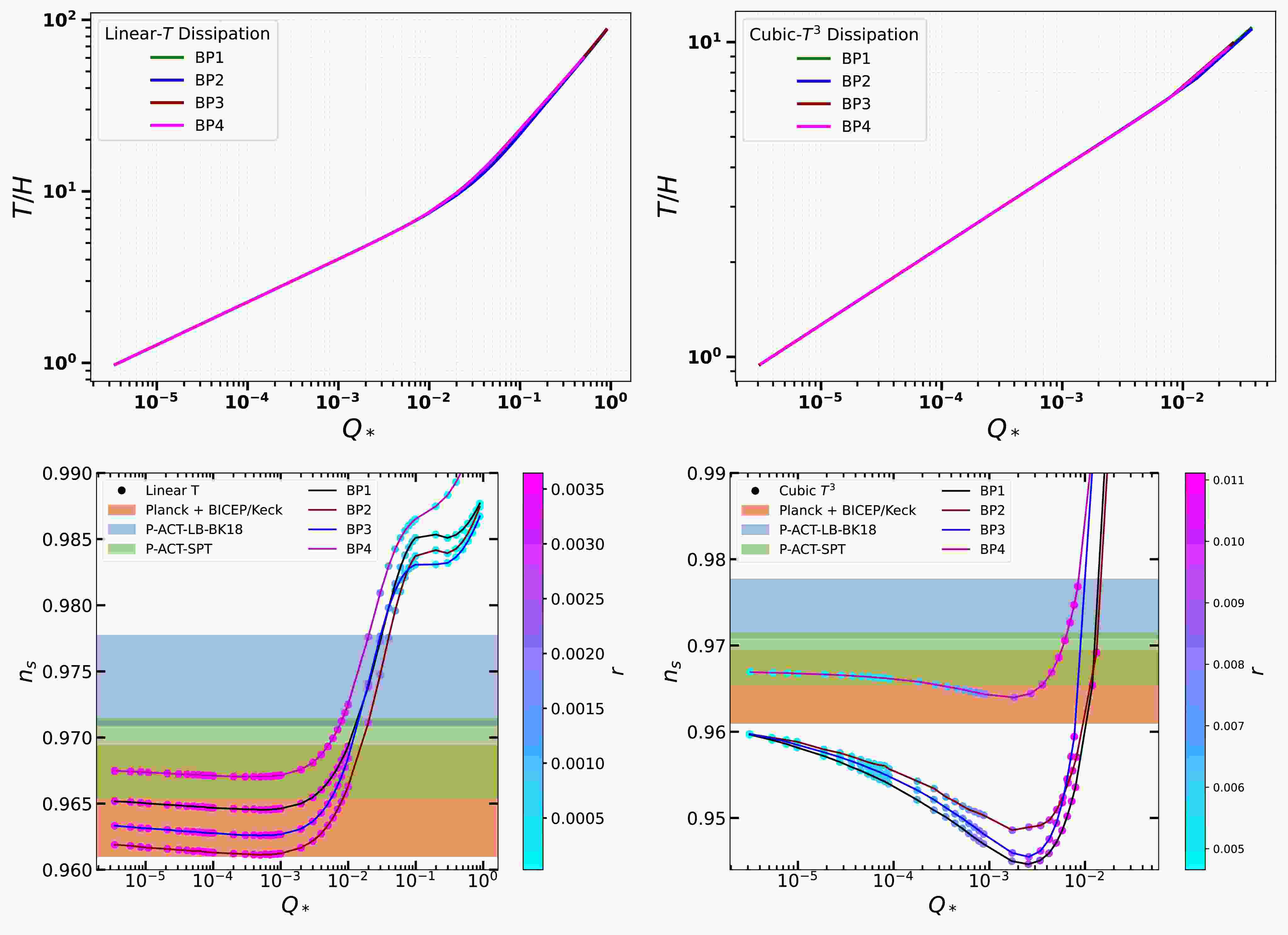
All numerical solutions are obtained using the $\mathrm{WI2easy}$ Mathematica code [46], a dedicated solver for warm inflation dynamics that integrates the background equations (29–32) together with the perturbation equations for scalar and tensor modes. The scalar power spectrum $ P_s $ and tensor power spectrum $ P_t $ are computed using the generalized warm inflation formalism [51, 60]. The scalar spectral index $ n_s $ and tensor-to-scalar ratio r are evaluated at the pivot scale $ k_* = 0.05\ {\rm{Mpc}}^{-1} $. We calibrate the potential amplitude using the measured value of $ P_s $ from Planck [14], which also fixes $ T^*/H^* $ for each benchmark point. We have verified the consistency of our $\mathrm{WI2easy}$ results with other warm inflation solvers such as $\mathrm{WI-easy}$ [46] and ensured numerical convergence across the parameter space.

To systematically explore the model predictions, we select four benchmark points (BP1–BP4) that span the weak, intermediate, and strong dissipative regimes. Their parameters are listed in Table 1. The main results are displayed in Fig. 1. The top panel illustrates the relationship between the dissipation ratio $ Q_* $ and the thermal ratio $ T_*/H_* $ across the full parameter space, revealing a transition at $ Q_* \simeq 3.5\times10^{-5} $. In the cold inflation regime ($ Q_* \lt 3.5 \times 10^{-5} $), $ T_*/H_* \lt 0.1 $, implying that the thermal bath is negligible compared to the Hubble scale, and quantum fluctuations dominate.

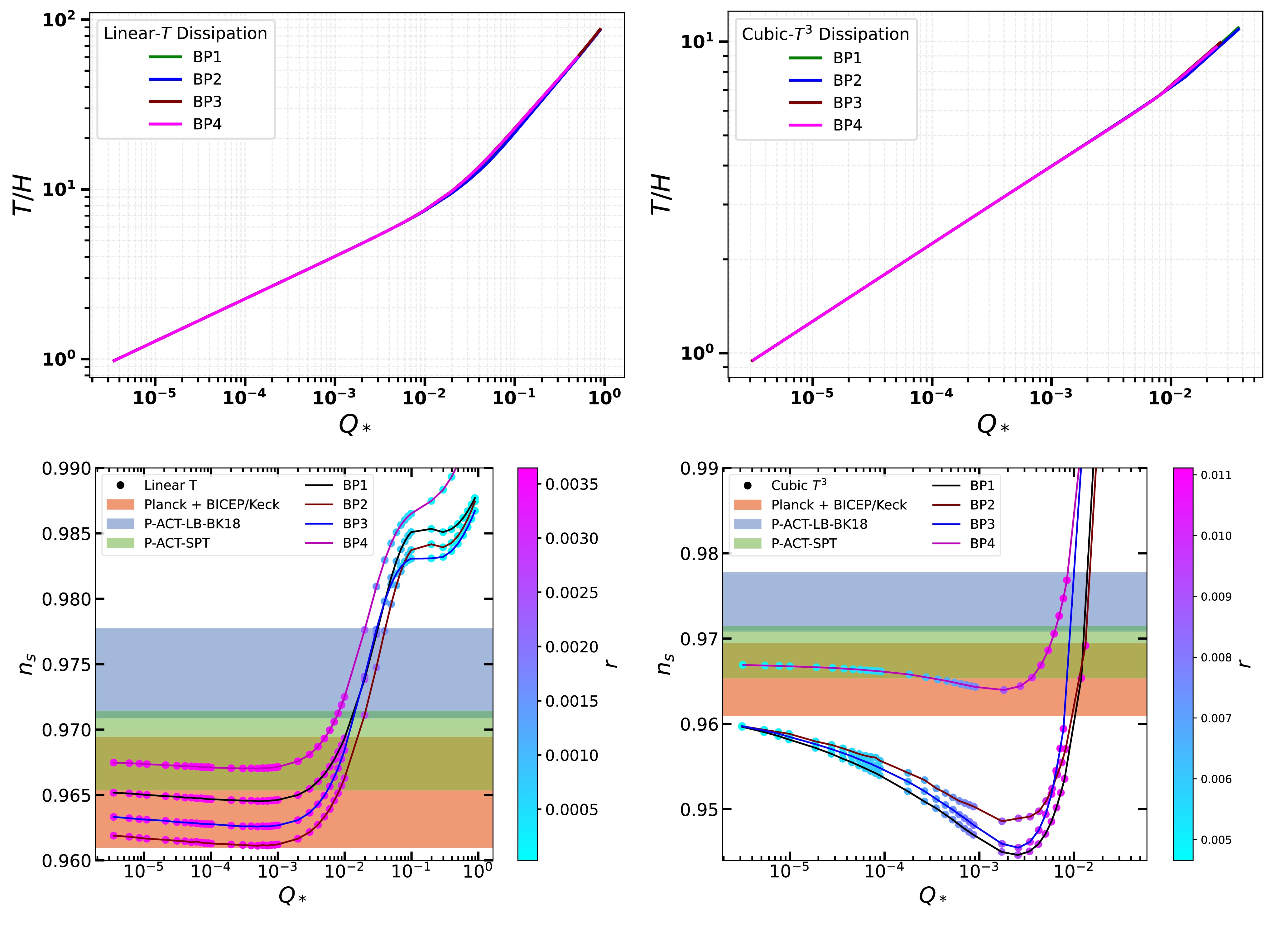
Figure 1.  (color online) The top panel shows the relationship between the dissipation ratio $ Q_* $ and the thermal ratio $ T_*/H_* $ for both linear ($ \Upsilon \propto T $) and cubic ($ \Upsilon \propto T^3 $) dissipation regimes, whereas the bottom panel shows the scalar spectral index $ n_s $ as a function of $ Q_* $ for linear dissipation (left) and cubic dissipation (right). For cubic dissipation, $ Q_* $ values above $ \sim10^{-2} $ are excluded because slow-roll breaks down and $ n_s $ exceeds observational bounds; therefore, the curves are truncated. The color bands represent the observational constraints from Planck+BICEP/Keck, P-ACT-LB-BK18, and SPT data. The four benchmark points (BP1–BP4) are indicated as colored trajectories.

In the transition region ($ 3.5\times 10^{-5} \lt Q_* $), $ 0.1 \lt T_*/H_* \lt 1 $, indicating that thermal effects are comparable to quantum effects. For the warm inflation regime ($ Q_* \gt 10^{-5} $), $ T_*/H_* \gt 1 $, so thermal fluctuations dominate over quantum fluctuations and significantly affect the inflaton dynamics. The thermal transition behavior differs between linear ($ \Upsilon \propto T $) and cubic ($ \Upsilon \propto T^3 $) dissipation forms. For linear dissipation, the transition is sharper at $ Q_* \simeq 2.8 \times 10^{-5} $, thermalization occurs faster due to linear temperature dependence, and the correlation between the thermal ratio and dissipation is $ T_*/H_* \propto Q_*^{0.85} $ for $ Q_* \gt 10^{-4} $. In contrast, cubic dissipation shows a broader transition centered at $ Q_* \simeq 4.2 \times 10^{-5} $, with slower initial thermalization but stronger temperature feedback, giving $ T_*/H_* \propto Q_*^{0.45} $ for $ Q_* \gt 10^{-4} $.

The bottom panel in Fig. 1 shows the scalar spectral index $ n_s $ as a function of the dissipative ratio at horizon crossing $ Q_* $ for both linear (left panel) and cubic (right panel) dissipation cases. The colored curves correspond to the four benchmark points, and the shaded regions represent the 68% and 95% confidence levels from combined CMB datasets (Planck+BK18, P-ACT-LB-BK18, SPT).

In the strict $ Q_*\to 0 $ limit, linear and cubic models converge to the same cold inflation predictions. The small difference seen in Fig. 1 at the smallest $ Q_* $ values is due to the different potential amplitudes $ V_0 $ required to fit $ P_s $ in each dissipation regime (see Table I). For all benchmarks, $ n_s $ asymptotically reaches a value $ \approx(0.96-0.965) $, which may be within the preferred range of Planck $ n_s = 0.9649 \pm 0.0042 $ [14]. However, these results for cold inflation fall outside the combined Planck and ACT DR4/DR6 (TT+TE+EE) bounds of $ n_s = 0.9743 \pm 0.01 $. Thus, cold inflation is not the best fit regime for our model, as it fails to match the observed spectral tilt of $ n_s = 0.9743 $ by P-ACT-LB-BK18.

For cubic dissipation, the function $ G(Q_*) $ grows as $ Q_*^{4.33} $ for large $ Q_* $, causing a rapid increase in the scalar power spectrum. For $ Q_* \gtrsim 10^{-2} $, the slow-roll conditions break down within the observable e-fold range, and the Planck normalization cannot be maintained while keeping $ n_s \lt 1 $. Hence, the curves are truncated at $ Q_* \sim 10^{-2} $. For linear dissipation, $ G(Q_*) $ increases more moderately, allowing slow-roll validity up to $ Q_* \sim 1 $.

As $ Q_* $ increases, dissipation becomes dynamically important. Both dissipation prescriptions initially exhibit a decrease in $ n_s $ for small $ Q_* $, but for large values, it turns around and starts to increase sharply. The rate of increase is steeper for the cubic case due to the stronger temperature dependence. For linear dissipation, $ n_s $ enters the 95% CL region around $ Q_* \sim 10^{-2} $; similarly, for cubic dissipation, this occurs at $ Q_* \sim 10^{-2} $. For $ Q_* \gg 0.01 $, both cases yield $ n_s \approx 0.97 $–$ 0.985 $, which is in excellent agreement with the observations of P-ACT-LB-BK18 and SPT.

The color bar in Fig. 1 shows the variation of the tensor-to-scalar ratio r. The opposite behavior of r with $ Q_* $ in linear vs. cubic dissipation can be traced to the different scalings of $ T_*/H_* $ and $ G(Q_*) $. For linear dissipation, $ T_*/H_* \propto Q_*^{0.85} $ and $ G(Q_*) $ grows slowly, so r decreases. For cubic dissipation, $ T_*/H_* \propto Q_*^{0.45} $ while $ G(Q_*) \propto Q_*^{4.33} $, leading to a relative enhancement of scalar power and a mild increase in r at large $ Q_* $.

The predicted range $ r \sim 10^{-3} $–$ 10^{-2} $ lies within the sensitivity reach of several upcoming and planned CMB polarization experiments. In particular, LiteBIRD [61, 62] targets a sensitivity of $ \sigma(r)\sim 10^{-3} $, while CMB-S4 [63] is expected to reach $ \sigma(r)\sim {\cal{O}}(10^{-4}) $, depending on delensing efficiency and foreground removal. In addition, ground-based and sub-orbital experiments such as the Simons Observatory [64] and the BICEP/Keck [15] program are expected to probe $ r \sim \text{few} \times 10^{-3} $, providing partial coverage of the upper end of the predicted range. Future concepts like CMB-HD may further improve sensitivity toward the $ 10^{-4} $ level. Therefore, a significant portion of the predicted parameter space is potentially testable, although a detection is not guaranteed and depends on foreground control and delensing performance.

All four benchmark points produce trajectories in the $ n_s $–$ Q_* $ plane that pass through the observationally allowed regions. Our results for $ n_s $ and r are similar to those of the warm little inflaton (WLI) framework [51], but our model offers a natural exit via the waterfall field and sub-Planckian field excursions due to the α-attractor geometry. More importantly, the hybrid structure lowers the required dissipation strength for consistency with ACT data. In single-field axion warm inflation, dissipation arises only from the axion–gauge field coupling $ \frac{\alpha}{4f}\phi F\tilde{F} $, giving $ \Upsilon \sim \alpha^2 T^3/f^2 $ and requiring $ Q_* \gtrsim 0.02 $ to match the observed $ n_s $ [48]. In our hybrid model, the inflaton additionally couples to the waterfall field via $ \frac{\lambda^2}{4}\phi^2\psi^2 $. Even when $ \psi=0 $ during inflation, virtual ψ fluctuations mediate extra energy transfer from ϕ to the thermal bath, effectively increasing the total dissipation coefficient. As a result, a smaller $ Q_* $ suffices to generate the same thermal noise. Quantitatively, for cubic dissipation, we find $ Q_* \gtrsim 0.008 $ in our model versus $ \gtrsim 0.02 $ in single-field models. Thus, the hybrid coupling provides an additional dissipation channel that reduces the threshold for warm inflation. This demonstrates the robustness of warm hybrid axion inflation: a wide range of dissipation strengths can yield predictions consistent with current CMB data. Notably, the cubic dissipation case allows for consistency at smaller $ Q_* $, reducing the required dissipation strength for agreement with Planck.

Similarly, in Fig. 2, we present the predictions for $ n_s $ as a function of $ \alpha_s $ for the same four benchmark points (BP1–BP4), with observational constraints overlaid from combined datasets (P-ACT-LB-BK18). As illustrated in Fig. 2, $ \alpha_s $ remains negative in the case of linear dissipation, while staying within the limits set by the combined datasets. In contrast, cubic dissipation spans a broader parameter space, allowing $ \alpha_s $ to vary from negative values up to approximately 0.015. All benchmark points produce predictions that lie within or close to the 95% confidence intervals of current combined CMB observations (P-ACT-LB), which constrain $ \alpha_s = 0.0062 \pm 0.0052 $ [13, 16].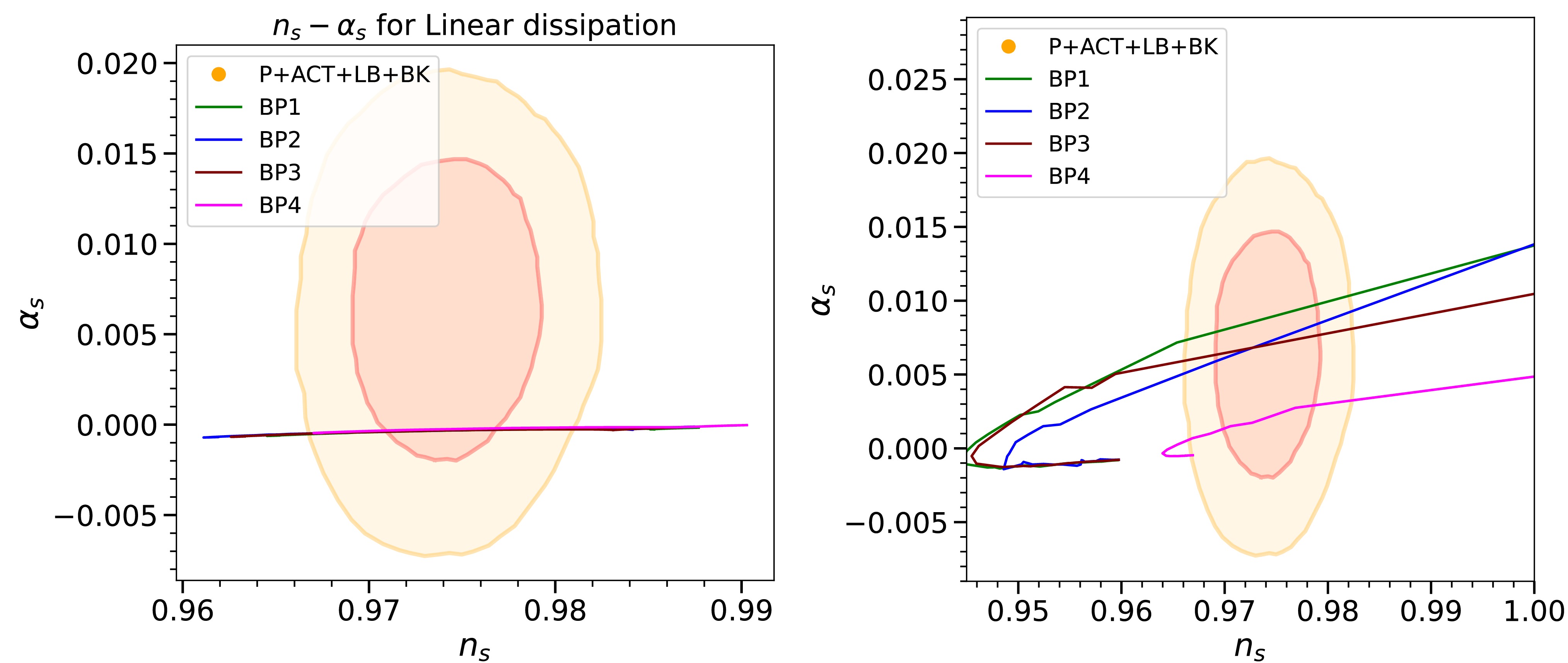

Figure 2.  (color online) Predictions for the $ n_s $ versus the running of the scalar spectral index $ \alpha_s $ for the four benchmark points (BP1–BP4) in linear dissipation (left) and cubic dissipation (right). Each curve is parameterized by the dissipation ratio $ Q_* $, increasing from left to right along the trajectory. The shaded regions correspond to the 68% and 95% confidence levels from combined CMB datasets: P-ACT-LB-BK18.

Before presenting the conclusions, we show the evolution of the inflaton field $ \phi(N) $ (left panel) together with the corresponding stability condition $ M_\psi^2 $ (right panel) for Benchmark Point 2 as a representative example in Fig. 3. This behavior is qualitatively similar for all other benchmark points.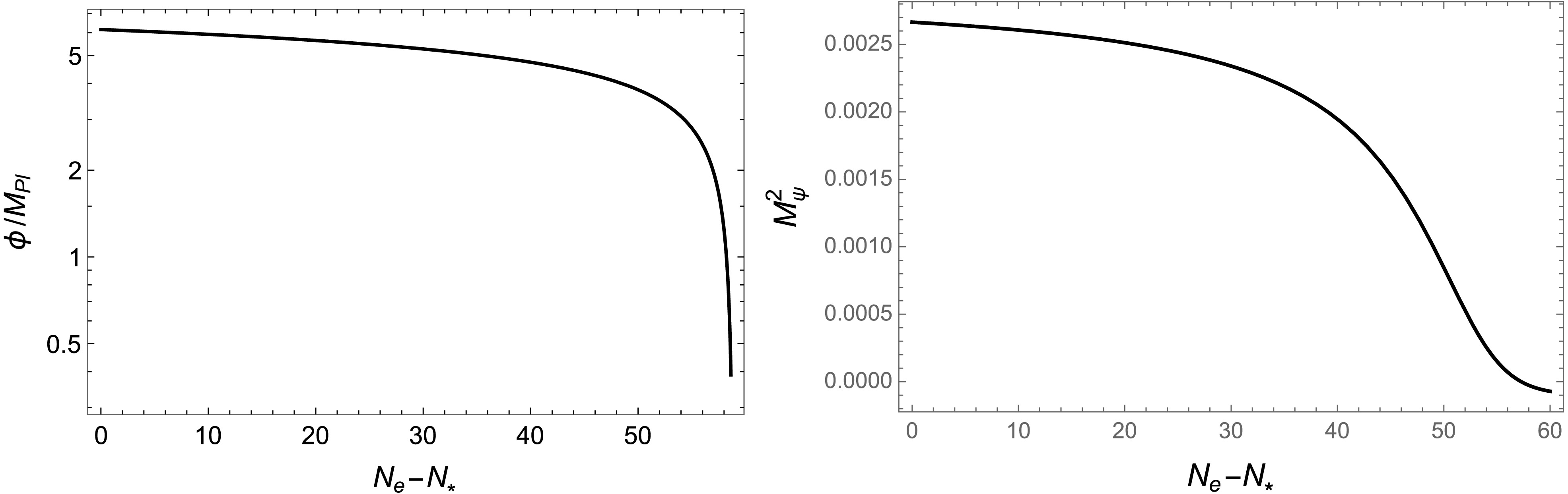

Figure 3.  Time evolution of the inflaton and stability condition for BP2 (linear dissipation). The left panel shows $ \phi(N) $, while the right panel shows $ M_\psi^2 $. The waterfall transition occurs near $ N \sim 55 $.

As shown in Fig. 3, the inflaton field undergoes a slow-roll evolution for $ N \lesssim 50 $, during which the condition $ M_\psi^2 \gt 0 $ is satisfied, ensuring that the trajectory $ \psi = 0 $ remains stable. As $ N \sim 55 $ is approached, the critical condition in Eq. (14) is reached, leading to the onset of a tachyonic instability in the waterfall field. This triggers a rapid transition that terminates inflation. These results confirm that all benchmark points consistently satisfy the required stability conditions throughout the inflationary evolution.

In this work, we have investigated warm hybrid axion inflation within the framework of α-attractor models. We considered a two-field scenario where the inflaton is an axion-like particle with a non-canonical kinetic term, and the waterfall field is responsible for ending inflation. The warm inflation dynamics are driven by dissipative effects, characterized by a dissipation coefficient Υ, which couples the inflaton to a thermal bath. We considered two forms of the dissipation coefficient: linear ($ \Upsilon \propto T $) and cubic ($ \Upsilon \propto T^3 $) in temperature.

Our numerical analysis, performed using the $\mathrm{W2easy}$ code, revealed that the model transitions from a cold inflation regime (disfavored by current data) to a warm inflation regime that is consistent with the latest CMB observations from Planck+BICEP/Keck, P-ACT-LB-BK18, and SPT. In particular, we found that for dissipative ratios $ Q_* \gtrsim 0.01 $, the scalar spectral index $ n_s $ falls within the 95% confidence region of the combined P-ACT-LB-BK18 data. The tensor-to-scalar ratio r is strongly suppressed in the warm regime, typically below $ 10^{-2}-10^{-3} $. Therefore, a significant portion of the predicted parameter space is potentially testable, although a detection is not guaranteed and depends on foreground control and delensing performance. Furthermore, the running of the scalar spectral index $ \alpha_s $ in the strong dissipative regime is also consistent with P-ACT-LB-BK18, which may be probed by future observations.