


 Abstract
 HTML
HTML Reference
 Related
 PDF
PDF


-
Core-collapse supernovae (CCSNe) are major astronomical neutrino sources since the collapse of the iron core of massive stars releases a gravitational energy of
$ \sim10^{53} $ ergs, with neutrinos carrying away most of this energy [1]. This explosive scenario has been confirmed by the detection of about two dozen neutrino events from SN1987A occurring in the Large Magellanic Cloud, with several Cherenkov detectors, including Kamiokande [2], Irvine–Michigan–Brookhaven Detectors [3], and the Mont Blanc Underground Neutrino Observatory [4].Neutrinos are essential in both the explosion dynamics and nucleosynthesis. The competition between neutrino heating and accretion onto the proto-neutron star (PNS) decides if the shock could successfully revive. However, neutrino transport from opaque to transparent regions is among the most crucial and challenging parts to model CCSN, owing to the large variety of scales involved and the fine spatial resolutions needed to obtain accurate results. One efficient way to model the neutrino transport is the leakage scheme [5−10]. It describes the neutrino spectrum as a Fermi-Dirac distribution with a local chemical potential
$ \mu_{\nu_{i}} $ for a neutrino species i. Neutrinos are approximately treated as they leak from the neutrinosphere$ R_{\nu_i} $ , which, by definition, is where the neutrino optical depth$ \tau_{\nu_i} $ equals$ 2/3 $ . On the other hand, the neutrino transport during the post-bounce phase determines the electron fraction ($ Y_e $ ) of the ejecta, which is a key parameter for nucleosynthesis in the later phase, especially for the rapid neutron-capture process [11, 12]. The emitted neutrinos from the neutrinosphere can further affect nucleosynthesis via the neutrino-nucleus reactions, i.e., the ν-process and νp-process [13−15]. The neutrino luminosities and spectra at the neutrinosphere are critical inputs for nucleosynthesis calculations, and these parameters are obtained from the neutrino transport during the explosion [16, 17].On the other hand, numerical studies have suggested that the magnetic field, especially the toroidal component near the newborn PNS surface, could possibly reach values up to
$ 10^{15-17} $ G [18−28], while the neutrino transport inside such a strong magnetic field is not well studied. The neutrino transport could be significantly altered due to the modification of weak interactions by the magnetic field, while few studies have focused on the impacts of magnetic fields on microscopic processes and the accompanying impacts on astrophysical sites: [29−31] studied the equation of state (EOS) under a strong magnetic field, [32] calculated the r-process nucleosynthesis considering impacts of a strong magnetic field on beta decay and electron-positron capture rates, and [33, 34] calculated the neutron star cooling under a strong magnetic field. Several previous studies investigated neutrino-nucleon interactions inside the magnetic field of PNS [35−37], but they did not investigate the effects in CCSN dynamical simulations. Recently, the magnetic field in the M1 neutrino transport scheme has been explored in both 3D Magnetohydrodynamical (MHD) CCSN simulations [38] and 1-D simulations for various magnetic field configurations [39]. For complementary purposes, in this study, we developed a formula that integrates the magnetic field effect with the leakage scheme. We set the magnetic field strengths from$ 10^{16} $ G to$ 10^{17} $ G. Our purpose is to explore how neutrino transport is modified in this strongly magnetized limit. We also emphasize that the present study does not include magnetic-pressure feedback on the hydrodynamics. Instead, we isolate the magnetic-field correction to neutrino transport as an additional physical effect that can be incorporated into future multidimensional MHD simulations.Compared to the M1 scheme used in previous studies, this method provides an effective way to estimate crucial physical properties of neutrinos, such as luminosity, neutrinosphere radius, and mean neutrino energy. This paper is arranged as follows. We show the impacts of the magnetic field on weak interactions in Section II. In Section III, we first describe the leakage scheme for neutrino transport and the corresponding adaptation for the presence of a strong magnetic field. Then, we present the numerical results of CCSN simulations and the impact of magnetic field strength on neutrino signals. In Section IV, we summarize the results.
-
Similar to our previous study on the M1 neutrino transport scheme [39], we apply the cross section from [35, 40] with the 0-th order of approximation:
$ \begin{aligned}[b] \sigma_{\nu{\rm{N}}}(E_n,B) =\;& \sigma_B^1\Big[1+2\chi \dfrac{(f\pm g)g }{ f^2 +3g^2} \cos \Theta_\nu\Big] \\ & +\sigma_B^2\Big[\dfrac{f^2 -g^2 }{ f^2 +3g^2}\cos\Theta_\nu + 2\chi \dfrac{(f\mp g) g }{ f^2 + 3g^2} \Big], \end{aligned} $
(1) where
$ \begin{aligned}[b] \sigma_B^1 =\;& \dfrac{G_F^2 \cos^2\theta_C }{ 2\pi}(f^2 + 3g^2) \\ &\times eB\sum^{n_{\rm{max}}}_{n=0}\sum^{s=1}_{s=-1}\dfrac{g_nE_n }{ \sqrt{E_n^2 - m_e^2 -(2n+s-1)eB}}, \end{aligned} $
(2) and
$ \begin{aligned} \sigma_B^2 = \dfrac{G_F^2 \cos^2\theta_C }{ 2\pi}(f^2 + 3g^2)eB\dfrac{E_n}{ \sqrt{E_n^2 - m_e^2}}. \end{aligned} $
(3) where
$ G_F = 1.166 \times 10^{-5} $ GeV−2 is the Fermi coupling constant, and$ \theta_C $ is the Cabibbo angle, for which we set the value$ \cos^2(\theta_C) = 0.95 $ . The vector and axial-vector coupling coefficients are$ f = 1 $ and$ g = 1.26 $ , respectively.$ E_n $ is the quantized electron energy given by$ E_n^2 = p_z^2 + m_e^2 + (2n + s - 1)eB $ , where n is the Landau quantum number [41], and s refers to the spin of$ e^\pm $ , i.e.,$ s=1 $ ($ s=-1 $ ) corresponds to the spin parallel (antiparallel) to the magnetic field. In Eq. 1, the upper sign is for the$ \nu_e + n $ reaction, and the lower sign is for$ \bar{\nu}_e + p $ .$ \Theta_\nu $ is the angle between the neutrino momentum and the magnetic field. As we will show, this angular-dependence in the cross section can be neglected, and we set$ \Theta_\nu = 0 $ throughout this work.Inside the magnetic field,
$ e^\pm $ obey the Fermi-Dirac distribution but with the Landau quantization of$ E_n $ , meaning that the chemical potential$ \mu_e $ also needs a correction.$ \mu_e $ is evaluated from the charge neutrality of the plasma, i.e., the net number density of both electrons and positrons should be balanced with the ions, where$ N_A $ is Avogadro's number. For a magnetized plasma, the momentum space of$ e^\pm $ is quantized as$ \begin{aligned}[b] &2\dfrac{d^3p}{ (2\pi)^3} f_{\rm{FD}}(E_e,\pm\mu_e;T)\\ &\to eB\sum^{\infty}_{n=0} (2-\delta_{n0}) \dfrac{dp_z}{ 4\pi^2}f_{\rm{FD}}(E_n,\pm\mu_e;T), \end{aligned} $
(4) Then, the net electron number density is given by
$ \begin{aligned}[b] \rho N_A Y_e = \;&n_e = \frac{m_e\omega_c}{(2\pi)^2}\sum_0^{n_{\rm{max}}} \int d {\bf{p}} \Big[f_{\rm{FD}}(E_n, +\mu_e; T)_{s=-1}\\ &+f_{\rm{FD}}(E_n, + \mu_e; T)_{s=1} - f_{\rm{FD}}(E_n, -\mu_e; T)_{s=-1}\\ &-f_{\rm{FD}}(E_n, -\mu_e; T)_{s=1}\Big]. \end{aligned} $
(5) Here,
$ \omega_c = eB/m_e $ is the cyclotron frequency, and$ s = \pm1 $ represents the spin state of$ e^\pm $ . Notice that inside the magnetic field, the spin is either parallel or antiparallel to the magnetic field.The upper panel of Fig.1 shows the chemical potential as a function of magnetic field strength at different temperatures. We set
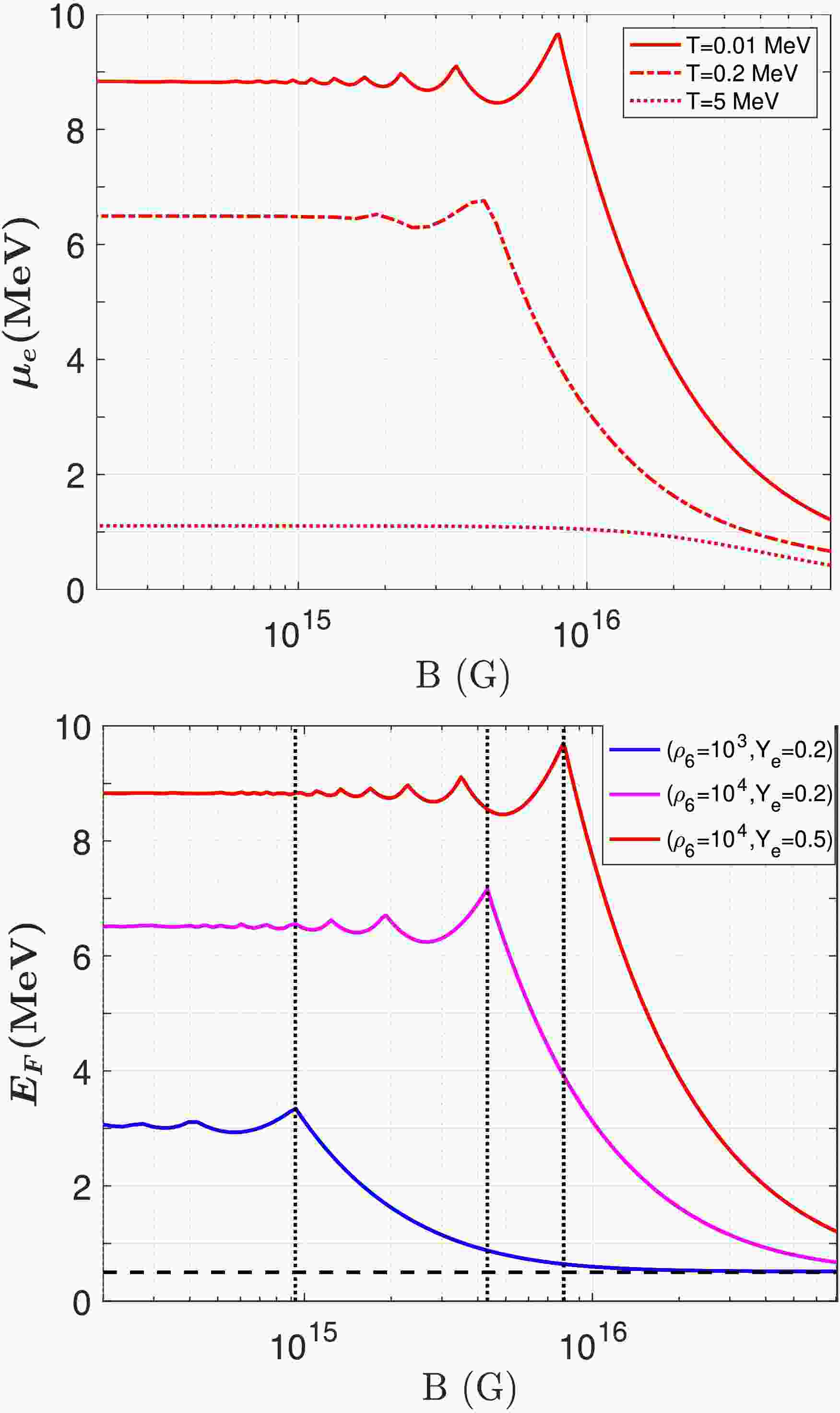
$ \rho_6\equiv \rho/10^6 \ \rm g\, cm^{-3} = 10^4 $ and$ Y_e=0.5 $ in this panel. In general, the chemical potential increases as temperature decreases (from the dotted line to the solid line in the upper panel of Fig. 1). For an extremely low temperature, Eq. 5 will recover the degenerate case, i.e., the red solid lines in both panels are identical to each other (the temperature is set to be zero in the bottom panel of Fig. 1).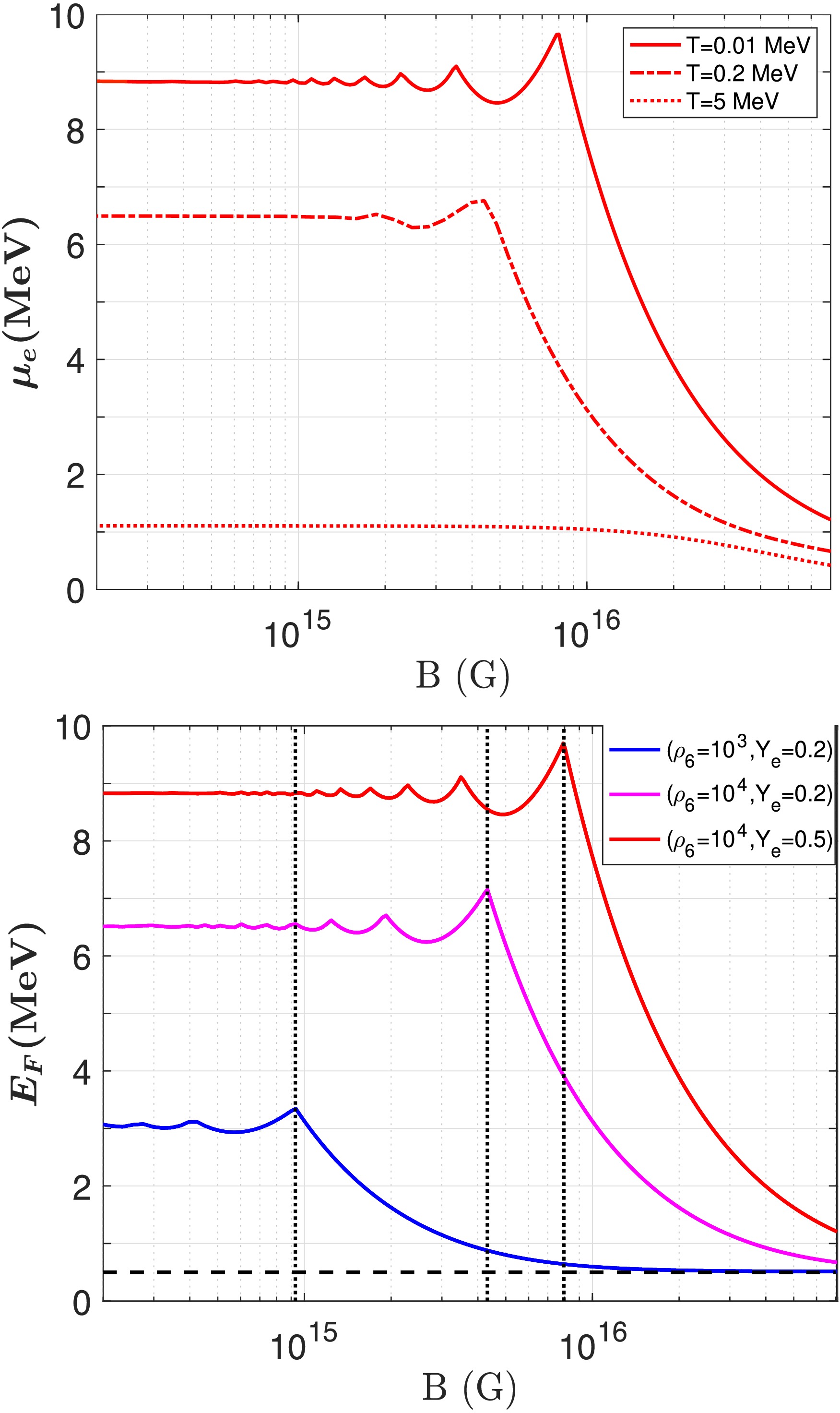
Figure 1. (color online) Upper panel: The chemical potential as a function of magnetic field strength for different temperatures, with
$ \rho = 10^{10} \;{\rm{g}}\; {\rm{cm}}^{-3} $ and$ Y_e = 0.5 $ . The solid line, dashed line, and dotted line correspond to$ T=0.01\ {\rm{MeV}} $ ,$ T=0.2\ {\rm{MeV}} $ , and$ T=5\ {\rm{MeV}} $ , respectively. The solid line is consistent with the red line on the lower panel since under this density and temperature, electrons are already in a degenerate state. Lower panel: Fermi energy$ E_F $ as a function of magnetic field strength with$ \rho_6 $ ,$ Y_e $ for different combinations as$ (10^3, 0.2) $ ,$ (10^4, 0.2) $ , and$ (10^4, 0.5) $ , respectively. If the magnetic field is relatively weak,$ E_F $ becomes the same as in a field-free case. On the other hand,$ E_F $ approaches$ m_e=0.511 $ MeV (horizontal dashed line) when$ B>B_{\rm{crit}} $ . Vertical dotted lines represent the value of$ B_{\rm{crit}} $ in each set of ρ and T.On the other hand, the chemical potential is reduced with increasing magnetic field strength. This is due to the extra energy contributed from the field to
$ e^\pm $ . In the case of strong fields,$ e^\pm $ only occupy the lowest Landau level (LLL), so that$ \mu_e $ decreases monotonically as a function of B and approaches the asymptotic value$ m_e $ for an extremely strong magnetic field. In the case of degenerate plasma, the critical magnetic field strength$ B_{\rm{crit}} $ for the scenario in which only the LLL is occupied reads [42].$ \begin{aligned} B_{\rm{crit}}=\frac{\pi}{e}\Big[2\pi(\rho Y_e)^2\Big]^{1/3}. \end{aligned} $
(6) When the magnetic field strength is below
$ B_{\rm{crit}} $ ,$ E_F $ shows a zig-zag pattern (bottom panel of Fig.1). The reason is as follows. For an extremely strong magnetic field, only the lowest Landau level (LLL) is occupied. As the magnetic-field strength decreases, higher Landau levels become accessible one after another. Whenever a new Landau level starts to be populated, the available phase space increases, and the Fermi energy$ E_F $ decreases accordingly for a fixed electron number density. Between two such thresholds, this readjustment becomes weaker, and$ E_F $ increases again more smoothly. This pattern is repeated whenever the next Landau level appears, leading to the oscillation-like behavior. We note that this behavior is consistent with Ref. [42], where only the zero-temperature Fermi energy$ E_F $ was discussed. In the present work, we extend their formulation to the finite-temperature case. For a weak magnetic field ($ B<10^{15} $ G),$ E_F $ values recover to the non-magnetized plasma cases:$ E_F=3.01 $ MeV (blue line), 6.51 MeV (pink line), and 8.82 MeV (red line) for the$ (\rho_6, Y_e) $ combinations we chose. -
Similar to our previous study on the M1 neutrino transport scheme [39], we apply the cross section from [35, 40] with the 0-th order of approximation:
$ \begin{aligned}[b] \sigma_{\nu{\rm{N}}}(E_n,B) =\;& \sigma_B^1\Big[1+2\chi \dfrac{(f\pm g)g }{ f^2 +3g^2} \cos \Theta_\nu\Big] \\ & +\sigma_B^2\Big[\dfrac{f^2 -g^2 }{ f^2 +3g^2}\cos\Theta_\nu + 2\chi \dfrac{(f\mp g) g }{ f^2 + 3g^2} \Big], \end{aligned} $
(1) where
$ \begin{aligned}[b] \sigma_B^1 =\;& \dfrac{G_F^2 \cos^2\theta_C }{ 2\pi}(f^2 + 3g^2) \\ &\times eB\sum^{n_{\rm{max}}}_{n=0}\sum^{s=1}_{s=-1}\dfrac{g_nE_n }{ \sqrt{E_n^2 - m_e^2 -(2n+s-1)eB}}, \end{aligned} $
(2) and
$ \begin{aligned} \sigma_B^2 = \dfrac{G_F^2 \cos^2\theta_C }{ 2\pi}(f^2 + 3g^2)eB\dfrac{E_n}{ \sqrt{E_n^2 - m_e^2}}. \end{aligned} $
(3) Where
$ G_F = 1.166 \times 10^{-5} $ GeV−2 is the Fermi coupling constant, and$ \theta_C $ is the Cabibbo angle, for which we set the value$ \cos^2(\theta_C) = 0.95 $ . The vector and axial-vector coupling coefficients are$ f = 1 $ and$ g = 1.26 $ , respectively.$ E_n $ is the quantized electron energy given by$ E_n^2 = p_z^2 + m_e^2 + (2n + s - 1)eB $ , where n is the Landau quantum number [41], and s refers to the spin of$ e^\pm $ , i.e.,$ s=1 $ ($ s=-1 $ ) corresponds to the spin parallel (antiparallel) to the magnetic field. In Eq. (1), the upper sign is for the$ \nu_e + n $ reaction, and the lower sign is for$ \bar{\nu}_e + p $ .$ \Theta_\nu $ is the angle between the neutrino momentum and the magnetic field. As we will show, this angular-dependence in the cross section can be neglected, and we set$ \Theta_\nu = 0 $ throughout this work.Inside the magnetic field,
$ e^\pm $ obey the Fermi-Dirac distribution but with the Landau quantization of$ E_n $ , meaning that the chemical potential$ \mu_e $ also needs a correction.$ \mu_e $ is evaluated from the charge neutrality of the plasma, i.e., the net number density of both electrons and positrons should be balanced with the ions, where$ N_A $ is Avogadro's number. For a magnetized plasma, the momentum space of$ e^\pm $ is quantized as$ \begin{aligned}[b] & 2\dfrac{\mathrm{d}^3p}{(2\pi)^3}f_{\rm{FD}}(E_e,\pm\mu_e;T) \\ & \to eB\sum_{n=0}^{\infty}(2-\delta_{n0})\dfrac{\mathrm{d}p_z}{4\pi^2}f_{\rm{FD}}(E_n,\pm\mu_e;T).\end{aligned} $
(4) Then, the net electron number density is given by
$ \begin{aligned}[b] \rho N_A Y_e = \;&n_e = \frac{m_e\omega_c}{(2\pi)^2}\sum_0^{n_{\rm{max}}} \int {\mathrm{d}} {\boldsymbol{p}} \Big[f_{\rm{FD}}(E_n, +\mu_e; T)_{s=-1}\\ &+f_{\rm{FD}}(E_n, + \mu_e; T)_{s=1} - f_{\rm{FD}}(E_n, -\mu_e; T)_{s=-1}\\ &-f_{\rm{FD}}(E_n, -\mu_e; T)_{s=1}\Big]. \end{aligned} $
(5) Here,
$ \omega_c = eB/m_e $ is the cyclotron frequency, and$ s = \pm1 $ represents the spin state of$ e^\pm $ . Notice that inside the magnetic field, the spin is either parallel or antiparallel to the magnetic field.The upper panel of Fig.1 shows the chemical potential as a function of magnetic field strength at different temperatures. We set
$ \rho_6\equiv \rho/10^6 \ \rm g\, cm^{-3} = 10^4 $ and$ Y_e=0.5 $ in this panel. In general, the chemical potential increases as temperature decreases (from the dotted line to the solid line in the upper panel of Fig. 1). For an extremely low temperature, Eq. (5) will recover the degenerate case, i.e., the red solid lines in both panels are identical to each other (the temperature is set to be zero in the bottom panel of Fig. 1).
Figure 1. (color online) Upper panel: The chemical potential as a function of magnetic field strength for different temperatures, with
$ \rho = 10^{10} \;{\rm{g}}\; {\rm{cm}}^{-3} $ and$ Y_e = 0.5 $ . The solid line, dashed line, and dotted line correspond to$ T=0.01\ {\rm{MeV}} $ ,$ T=0.2\ {\rm{MeV}} $ , and$ T=5\ {\rm{MeV}} $ , respectively. The solid line is consistent with the red line on the lower panel since under this density and temperature, electrons are already in a degenerate state. Lower panel: Fermi energy$ E_F $ as a function of magnetic field strength with$ \rho_6 $ ,$ Y_e $ for different combinations as$ (10^3, 0.2) $ ,$ (10^4, 0.2) $ , and$ (10^4, 0.5) $ , respectively. If the magnetic field is relatively weak,$ E_F $ becomes the same as in a field-free case. On the other hand,$ E_F $ approaches$ m_e=0.511 $ MeV (horizontal dashed line) when$ B>B_{\rm{crit}} $ . Vertical dotted lines represent the value of$ B_{\rm{crit}} $ in each set of ρ and T.On the other hand, the chemical potential is reduced with increasing magnetic field strength. This is due to the extra energy contributed from the field to
$ e^\pm $ . In the case of strong fields,$ e^\pm $ only occupy the lowest Landau level (LLL), so that$ \mu_e $ decreases monotonically as a function of B and approaches the asymptotic value$ m_e $ for an extremely strong magnetic field. In the case of degenerate plasma, the critical magnetic field strength$ B_{\rm{crit}} $ for the scenario in which only the LLL is occupied reads [42].$ \begin{aligned} B_{\rm{crit}}=\frac{\pi}{e}\Big[2\pi(\rho Y_e)^2\Big]^{1/3}. \end{aligned} $
(6) When the magnetic field strength is below
$ B_{\rm{crit}} $ ,$ E_F $ shows a zig-zag pattern (bottom panel of Fig.1). The reason is as follows. For an extremely strong magnetic field, only the lowest Landau level (LLL) is occupied. As the magnetic-field strength decreases, higher Landau levels become accessible one after another. Whenever a new Landau level starts to be populated, the available phase space increases, and the Fermi energy$ E_F $ decreases accordingly for a fixed electron number density. Between two such thresholds, this readjustment becomes weaker, and$ E_F $ increases again more smoothly. This pattern is repeated whenever the next Landau level appears, leading to the oscillation-like behavior. We note that this behavior is consistent with Ref. [42], where only the zero-temperature Fermi energy$ E_F $ was discussed. In the present work, we extend their formulation to the finite-temperature case. For a weak magnetic field ($ B<10^{15} $ G),$ E_F $ values recover to the non-magnetized plasma cases:$ E_F=3.01 $ MeV (blue line), 6.51 MeV (pink line), and 8.82 MeV (red line) for the$ (\rho_6, Y_e) $ combinations we chose. -
In the leakage scheme, one can calculate the optical depth from the integration of local opacity
$ \kappa_{\rm{tot}} $ , which is determined by the local mean free path of neutrinos or, equivalently, by the interaction rates of the neutrino processes (scattering, absorption, and emission). The total opacity$ \kappa_{\rm{tot}} $ of electron-type neutrinos is given by [10].$ \begin{aligned} &\kappa_{{\rm{ tot}},j}(\nu_e) = \kappa_{a,j}(\nu_e n)+ \kappa_{s,j}(\nu_e n) + \kappa_{s,j}(\nu_e p) \end{aligned} $
(7) $ \begin{aligned} &\kappa_{{\rm{ tot}},j}(\bar{\nu}_e) = \kappa_{a,j}(\bar{\nu}_e p)+ \kappa_{s,j}(\bar{\nu}_e n) + \kappa_{s,j}(\bar{\nu}_e p), \end{aligned} $
(8) Where a represents the absorption process and s stands for the scattering process. Index j is introduced to denote the opacities for neutrino-number transport (
$ j=0 $ ) and neutrino-energy transport ($ j=1 $ ), respectively. As discussed in Sec. II, inside a magnetic field, the absorption cross sections differ from the field-free case, and the absorption opacities of$ {\nu}_e $ and$ \bar{\nu}_e $ are given by$ \begin{aligned}[b] &\kappa^B_{a,j}(\nu_e n)=A\rho Y_{\rm{np}}\times\\ &\frac{ \int_0^\infty dE_{\nu_e}\sigma(E_n,B)E_{\nu_e}^{2+j} f_{\rm{FD}}(E_{\nu_e},\eta_{\nu_e}; T_{\nu_e}) g\Big[E_n,\mu_e(B);T_e\Big] } {\int_0^\infty dE_{\nu_e} E_{\nu_e}^{2+j} f_{\rm{FD}}(E_{\nu_e},\eta_{\nu_e}; T_{\nu_e})},\\ \end{aligned} $
(9) $ \begin{aligned}[b] &\kappa^B_{a,j}(\bar{\nu}_e p) = A\rho Y_{\rm{pn}}\times \\ &\frac{\begin{aligned}\int_0^\infty dE_{\bar{\nu}_e}\sigma(E_{n},B)E_{\bar{\nu}_e}^{2+j} f_{\rm{FD}}(E_{\bar{\nu}_e},\eta_{\bar{\nu}_e}; T_{\bar{\nu}_e}) g\Big[E_n,-\mu_e(B);T_{e}\Big]\end{aligned}}{\begin{aligned}\int_0^\infty dE_{\bar{\nu}_e} E_{\bar{\nu}_e}^{2+j} f_{\rm{FD}}(E_{\bar{\nu}_e},\eta_{\bar{\nu}_e}; T_{\bar{\nu}_e})\end{aligned}}, \end{aligned} $
(10) where
$ \eta_{\nu_e} = \mu_{\nu_e}/k_BT $ is the neutrino degeneracy parameter (the same definition applies for$ \eta_{\bar{\nu}_e} $ ),$ \sigma(E_n,B) $ is taken from Eq. 1, and the electron chemical potential$ \mu_e(B) $ is calculated from Eq. 5.$ g(E_n,\mu_e;T_e) $ is the Pauli blocking factor for a Fermion.$ Y_{\rm{np}} $ and$ Y_{\rm{pn}} $ are coefficients that include the Pauli blocking effects in the phase space of neutrons and protons (see Appendix A for these expressions). Since the magnetic moment of nucleons is negligible due to their heavy mass, we ignore the impacts on neutrino scattering processes. One can find the expressions for the cross section and opacity in [10]. For heavy-lepton neutrinos (i.e.,$ \nu_\tau $ and$ \nu_\mu $ ), only scattering processes are included:$ \begin{aligned} \kappa_{{\rm{tot}},j}(\nu_x) = \kappa_{s,j}(\nu_x n) + \kappa_{s,j}(\nu_x p). \end{aligned} $
(11) Finally, the optical depth is given by
$ \begin{aligned} \tau_{\nu_i,j}(r)=\int^{\infty}_{r} ds\ \kappa_{{\rm{tot}}, j}(\nu_i), \end{aligned} $
(12) and the neutrinosphere, by definition, is given by
$ \tau_{\nu_i,j}(R_\nu) = 2/3 $ . Other quantities in the leakage scheme, such as local emission and absorption rates and effective emission and absorption rates, are also modified in terms of an external magnetic field. We include these equations in Appendix B. In this work, we use the open-source${\tt{GR1D}} $ code to simulate 1-D SNe explosions [43, 44]. We used the LS180 EOS [45] and took a 9.6 M⊙ progenitor model with zero metallicity from [46]. The collapse phase employs the parameterization scheme for electron captures following [47], and we switch to the leakage scheme after the core bounce, defined as the moment when the entropy per baryon at the edge of the inner core reaches 3$ k_{\rm{B}} $ .We also note that our 1D simulations do not include magnetic pressure or other magnetic feedback on the hydrodynamics. For magnetic fields of this strength, such effects could substantially modify the hydrodynamical evolution. In the present work, however, we focus only on the magnetic-field correction to neutrino transport, which should be regarded as an additional effect beyond the hydrodynamics.
-
In the leakage scheme, one can calculate the optical depth from the integration of local opacity
$ \kappa_{\rm{tot}} $ , which is determined by the local mean free path of neutrinos or, equivalently, by the interaction rates of the neutrino processes (scattering, absorption, and emission). The total opacity$ \kappa_{\rm{tot}} $ of electron-type neutrinos is given by [10].$ \begin{aligned} &\kappa_{{\rm{ tot}},j}(\nu_e) = \kappa_{a,j}(\nu_e n)+ \kappa_{s,j}(\nu_e n) + \kappa_{s,j}(\nu_e p) \end{aligned} , $
(7) $ \begin{aligned} &\kappa_{{\rm{ tot}},j}(\bar{\nu}_e) = \kappa_{a,j}(\bar{\nu}_e p)+ \kappa_{s,j}(\bar{\nu}_e n) + \kappa_{s,j}(\bar{\nu}_e p), \end{aligned} $
(8) where a represents the absorption process and s stands for the scattering process. Index j is introduced to denote the opacities for neutrino-number transport (
$ j=0 $ ) and neutrino-energy transport ($ j=1 $ ), respectively. As discussed in Sec. II, inside a magnetic field, the absorption cross sections differ from the field-free case, and the absorption opacities of$ {\nu}_e $ and$ \bar{\nu}_e $ are given by$ \begin{aligned}[b] &\kappa^B_{a,j}(\nu_e n)=A\rho Y_{{np}}\\ &\times\frac{\displaystyle \int_0^\infty {\mathrm{d}}E_{\nu_e}\sigma(E_n,B)E_{\nu_e}^{2+j} f_{\rm{FD}}(E_{\nu_e},\eta_{\nu_e}; T_{\nu_e}) g\Big[E_n,\mu_e(B);T_e\Big] } {\displaystyle\int_0^\infty {\mathrm{d}}E_{\nu_e} E_{\nu_e}^{2+j} f_{\rm{FD}}(E_{\nu_e},\eta_{\nu_e}; T_{\nu_e})},\\ \end{aligned} $
(9) $ \begin{aligned}[b] &\kappa^B_{a,j}(\bar{\nu}_e p) = A\rho Y_{{pn}} \\ & \times\frac{\begin{aligned}\int_0^\infty {\mathrm{d}}E_{\bar{\nu}_e}\sigma(E_{n},B)E_{\bar{\nu}_e}^{2+j} f_{\rm{FD}}(E_{\bar{\nu}_e},\eta_{\bar{\nu}_e}; T_{\bar{\nu}_e}) g\Big[E_n,-\mu_e(B);T_{e}\Big]\end{aligned}}{\begin{aligned}\int_0^\infty {\mathrm{d}}E_{\bar{\nu}_e} E_{\bar{\nu}_e}^{2+j} f_{\rm{FD}}(E_{\bar{\nu}_e},\eta_{\bar{\nu}_e}; T_{\bar{\nu}_e})\end{aligned}}, \end{aligned} $
(10) where
$ \eta_{\nu_e} = \mu_{\nu_e}/k_BT $ is the neutrino degeneracy parameter (the same definition applies for$ \eta_{\bar{\nu}_e} $ ),$ \sigma(E_n,B) $ is taken from Eq. (1), and the electron chemical potential$ \mu_e(B) $ is calculated from Eq. (5).$ g(E_n,\mu_e;T_e) $ is the Pauli blocking factor for a Fermion.$ Y_{{np}} $ and$ Y_{{pn}} $ are coefficients that include the Pauli blocking effects in the phase space of neutrons and protons (see Appendix A for these expressions). Since the magnetic moment of nucleons is negligible due to their heavy mass, we ignore the impacts on neutrino scattering processes. One can find the expressions for the cross section and opacity in [10]. For heavy-lepton neutrinos (i.e.,$ \nu_\tau $ and$ \nu_\mu $ ), only scattering processes are included:$ \begin{aligned} \kappa_{{\rm{tot}},j}(\nu_x) = \kappa_{s,j}(\nu_x n) + \kappa_{s,j}(\nu_x p). \end{aligned} $
(11) Finally, the optical depth is given by
$ \begin{aligned}\tau_{\nu_i,j}(r)=\int_r^{\infty}\mathrm{d}s\ \kappa_{\rm{tot},j}(\nu_i),\end{aligned} $
(12) and the neutrinosphere, by definition, is given by
$ \tau_{\nu_i,j}(R_\nu) = 2/3 $ . Other quantities in the leakage scheme, such as local emission and absorption rates and effective emission and absorption rates, are also modified in terms of an external magnetic field. We include these equations in Appendix B. In this work, we use the open-source${\tt{GR1D}} $ code to simulate 1-D SNe explosions [43, 44]. We used the LS180 EOS [45] and took a 9.6 M⊙ progenitor model with zero metallicity from [46]. The collapse phase employs the parameterization scheme for electron captures following [47], and we switch to the leakage scheme after the core bounce, defined as the moment when the entropy per baryon at the edge of the inner core reaches 3$ k_{\rm{B}} $ .We also note that our 1D simulations do not include magnetic pressure or other magnetic feedback on the hydrodynamics. For magnetic fields of this strength, such effects could substantially modify the hydrodynamical evolution. In the present work, however, we focus only on the magnetic-field correction to neutrino transport, which should be regarded as an additional effect beyond the hydrodynamics.
-
We first use the extracted density, temperature, and
$ Y_e $ profiles at a certain time step from the${\tt{GR1D}} $ code to clarify the magnetic field impacts inside CCSN. Fig. 2 illustrates the total opacity$ \kappa_{\rm{tot}} $ of neutrinos (blue lines, left y-axis) and antineutrinos (red lines, right y-axis) during different stages (1 ms, 50 ms, and 100 ms after core bounce, respectively) of CCSN. In the inner region of CCSN, neutrino scattering contributes the most to opacity, so the modification of absorption processes can be ignored.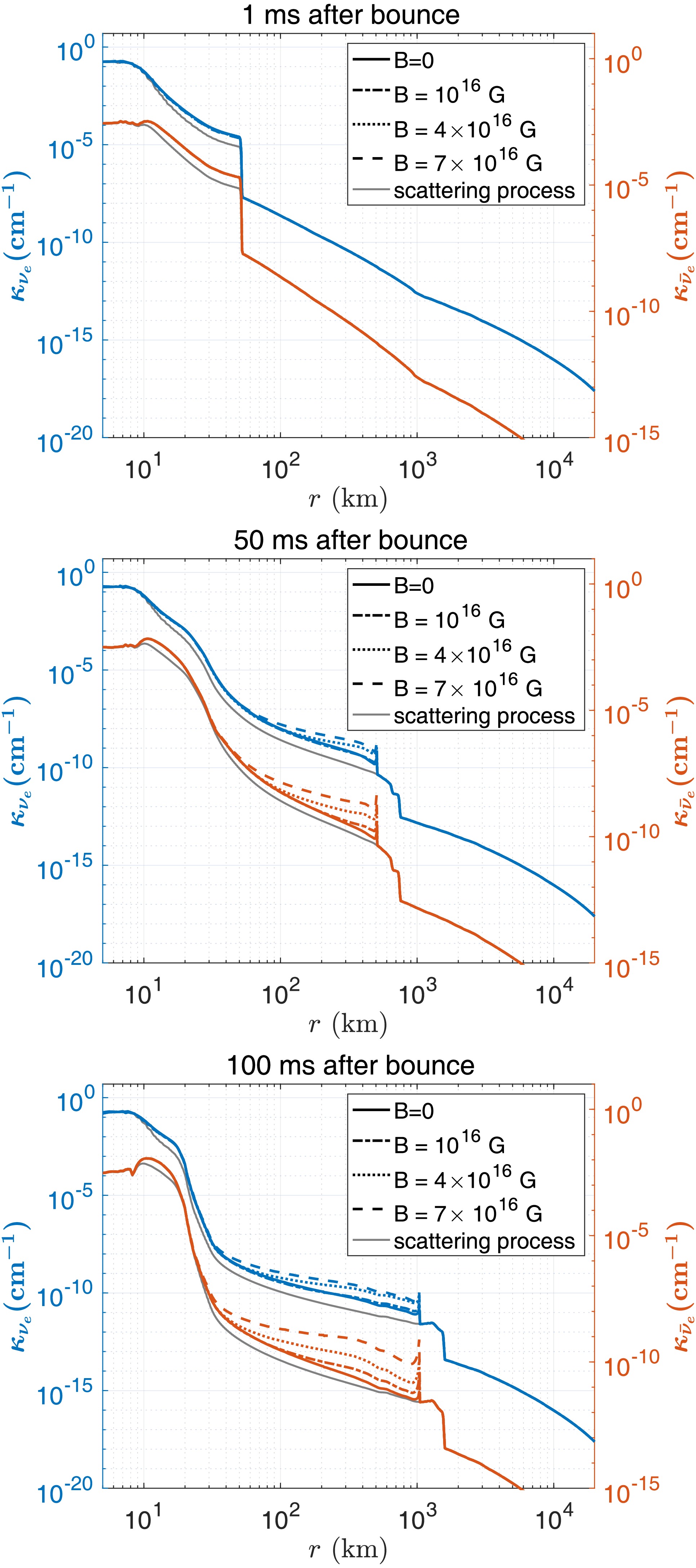
Figure 2. (color online) The opacity of
$ \nu_e $ and$ \bar{\nu}_e $ inside CCSN is compared at different stages: 1 ms, 50 ms, and 100 ms after core bounce. Blue lines represent the opacity for$ \nu_e $ , while red lines represent the opacity for$ \bar{\nu}_e $ . The gray solid lines on all panels show the opacity contributed by scattering processes:$ \nu_e + n(p) \to \nu_e + n(p) $ and$ \bar{\nu}_e + n(p) \to \bar{\nu}_e + n(p) $ . The line styles—solid, dash-dotted, dotted, and dashed—indicate the cases for$ B = 0 $ ,$ B = 10^{16} $ G,$ B = 4\times 10^{16} $ G, and$ B = 7\times 10^{16} $ G, respectively.At a very early phase after core bounce, the shock propagates in a high-density and high-temperature region, so the magnetic field does not make significant contributions, i.e., there is no difference between each line for various magnetic field strengths (upper panel of Fig. 2). The magnetic field enhances absorption opacity when the shock propagates to
$ r \geq 30 $ km (middle and lower panel of Fig. 2). This is mainly caused by two effects: 1) The magnetic field quantizes the phase space of$ e^\pm $ , with extra magnetic energy contribution, which enhances the neutrino-nucleon interaction rates. 2) The electron chemical potential$ \mu_e $ is suppressed since only the LLL is occupied, as we discussed in Sec. II, leading to a larger value of the blocking factor$ g(E_n,-\mu_e; T_e) $ than$ g(E_n,\mu_e; T_e) $ . These impacts are consistent with those in the M1 scheme, as we discussed in [39], i.e., both the cross section deviation and chemical potential modification have a more pronounced effect on$ \bar{\nu}_e $ , leading to a greater enhancement of$ \bar{\nu}_e $ opacity compared to that of$ \nu_e $ .At a relatively later stage (
$ t\sim 100 $ ms), the matter cools down, and the magnetic field could enhance opacity by about 2-3 orders of magnitude in the region 100 km$ <r< $ 1000 km inside CCSN (lower panel of Fig. 2). However, the optical depth in such a later phase is mainly determined by the opacity of the inner region ($ r<30 $ km) due to the sharp decay of opacity with radius. Therefore, the neutrinosphere would eventually become indistinguishable from the field-free scenario (see Fig. 5 below).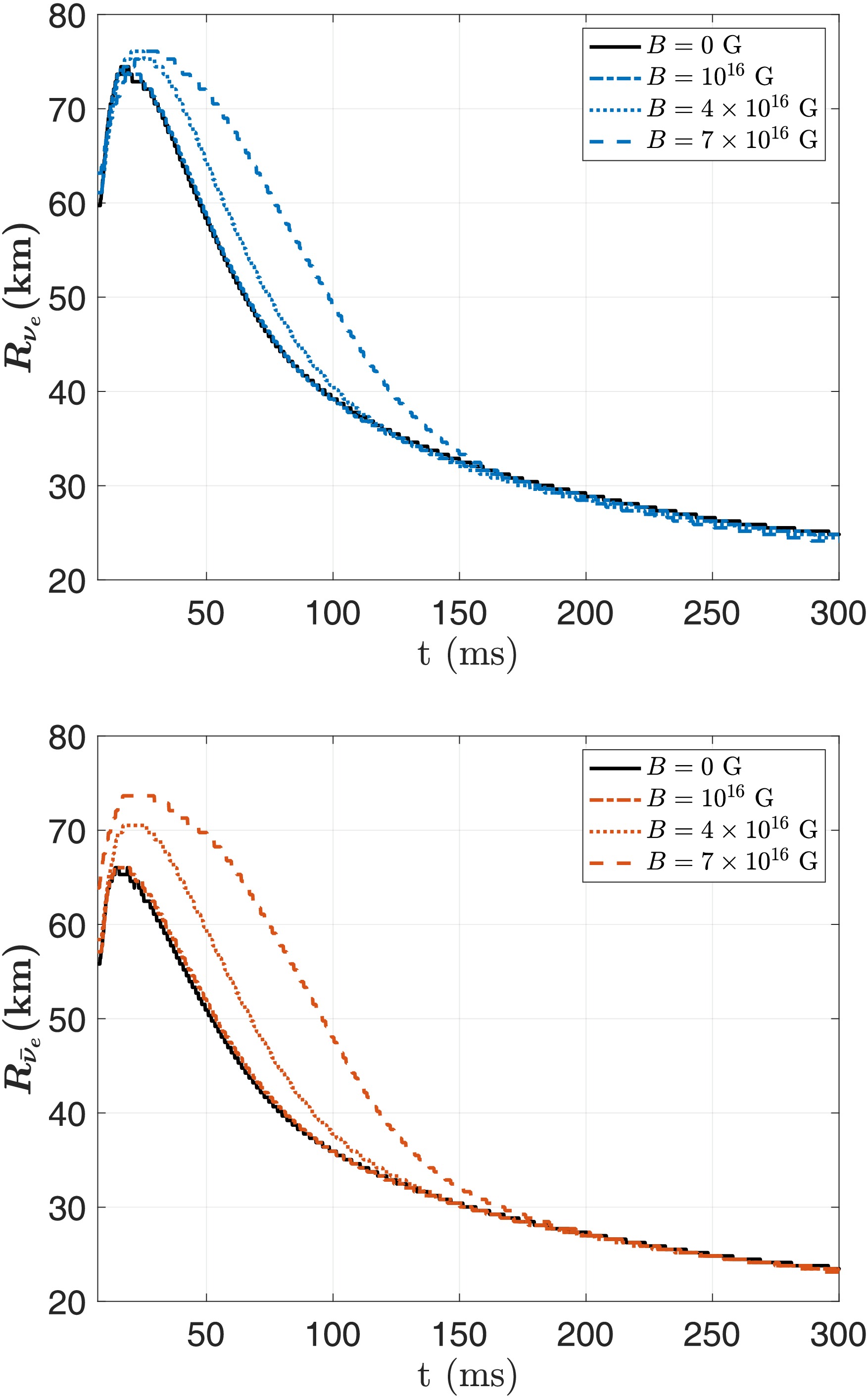
Figure 5. (color online) Upper panel: The neutrinosphere evolution (
$ \nu_e $ ) after core bounce. Lower panel: The neutrinosphere evolution of$ \bar{\nu}_e $ after core bounce. Black solid lines correspond to the field-free case; red, green, and blue lines correspond to$ B=10^{16} $ G,$ B=4\times 10^{16} $ G, and$ B=7\times 10^{16} $ G, respectively.Notice that in a more realistic dipole field case, the
$ \Theta_\nu $ in Eq. 1 depends on the neutrino momentum direction and field direction. We apply different$ \Theta_\nu $ values to calculate the angle dependence of$ \kappa_{abs}(\nu_e) $ as a function of$ \eta_{\nu_e} $ . The results are shown in Fig. 2. Here, the widths of the blue and yellow bands are caused by changing the value of$ \Theta_\nu $ from 0 to π. The temperature and density are set to be$ T=1 $ MeV and$ \rho= 10^9\rm \ g\cdot cm^{-3} $ . The absorption opacity can differ by a factor of 2 by changing the value of$ \Theta_\nu $ for$ B=10^{17} $ G. However, this is the upper limit of the magnetic field strength. The yellow band shows less than a 20% difference for the case of a$ 4\times10^{16} $ G magnetic field, indicating that neglecting the angular effect can be a reasonable approximation, so we set$ \Theta_\nu=0 $ throughout this work.The effective neutrino emission rates, as seen in Eq. B3, describe whether the neutrinos are diffused or emitted inside a CCSN. In a high-density regime, diffusion rates are high, which governs the main neutrino number and energy loss. In contrast, the main process becomes the local emission rate if neutrinos travel to a low-density region. We show the effective emission rates in Fig. 4 for different stages of a CCSN (from top to bottom panel: 1 ms, 50 ms, and 100 ms after the core bounce, respectively). Again, we compare the impacts of the magnetic field under the extracted density, temperature, and
$ Y_e $ conditions in this figure. About 50 ms after core bounce (middle panel of Fig. 4), a magnetic field suppresses the effective neutrino emission rates in the range of$ 30\ {\rm{km}}<r< 100 \ {\rm{km}} $ , due to the enhancement of opacity shown in the middle panel of Fig. 2. Also, this result is consistent with the reduction of the diffusion rates in this region (cf. Appendix B). At 100 ms after core bounce (lower panel of Fig. 4), the shock has already propagated to the outer region, so the matter cools down and has a lower density. Diffusion is not essential in such an environment, while the local emission rates are enhanced more drastically (cf. Appendix B), leading to stronger effective emission rates.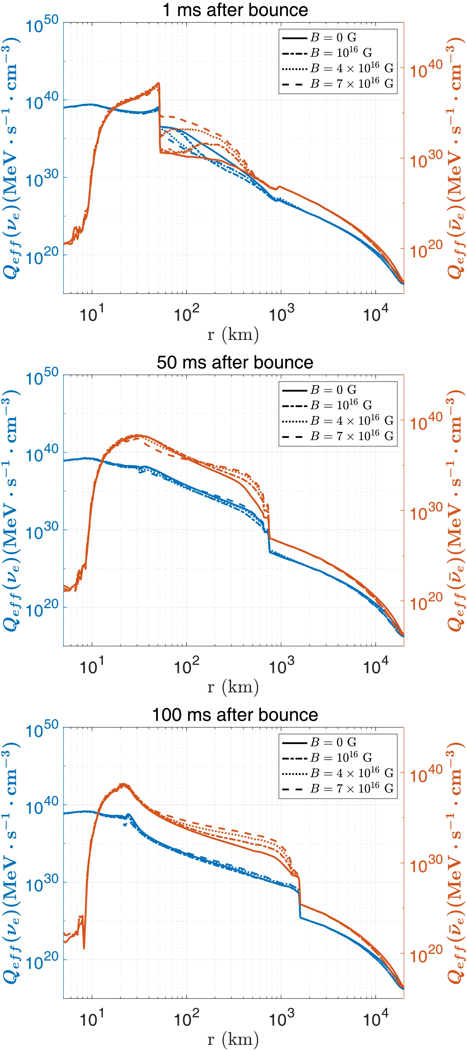
Figure 4. (color online) The effective energy emission rate of
$ \nu_e $ and$ \bar{\nu}_e $ inside the CCSN after the core bounce. The line-color convention follows Fig. 2.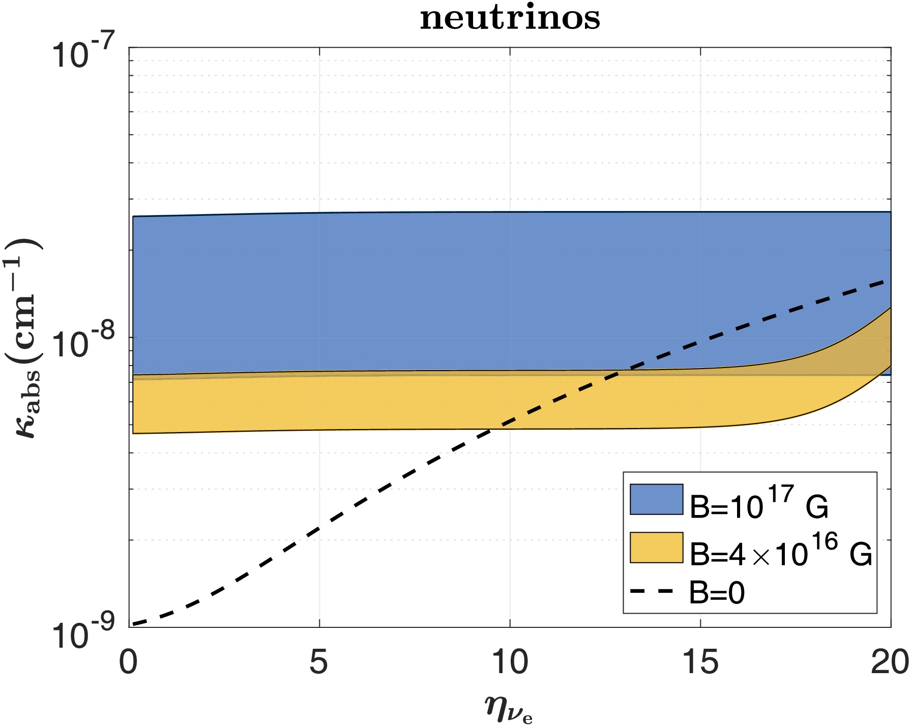
Figure 3. (color online) The neutrino absorption opacity
$ \kappa_{\rm{abs}} $ is considered under varying magnetic field strengths. The black solid line represents the field-free case. The blue band corresponds to a magnetic field strength of$ 10^{17} $ G, with different values of$ \Theta_\nu $ ; the lower boundary of the band represents$ \Theta_\nu=0 $ , while the upper boundary represents$ \Theta_\nu=\pi $ . Similarly, the yellow band corresponds to a magnetic field strength of$ 4\times 10^{16} $ G, with the same interpretation for the lower and upper boundaries. In this figure, the temperature is set at$ T=1 $ MeV and the density at$ \rho= 10^9\; {\rm{g}}\cdot {\rm{cm}}^{-3} $ .We further modified the neutrino transport in
${\tt{GR1D}} $ based on Eq. 9, Eq. 10, and equations in Appendix B to perform 1-D simulations with a magnetic field. We investigate the impacts of a constant magnetic field in a region$ r<r_{\rm{cut}}=100 $ km in our CCSN simulation. The enhanced opacity enlarges the radius of the neutrinosphere, which is shown in Fig. 5, where the time evolution of the neutrinosphere for$ \nu_e $ and$ \bar{\nu}_e $ are shown in the upper and lower panels, respectively (our calculation uses the opacity for neutrino-energy transport$ \kappa_{{\rm{tot}},1}(\nu_i) $ to determine the neutrinosphere). The radius of the neutrinosphere is indistinguishable under different magnetic field cases at$ t<10 $ ms after core bounce. After a few dozen milliseconds, when the shock propagates outside the high-density and high-temperature region,$ \kappa_{\rm{tot}} $ increases, and one can see the enlargement of the neutrinosphere as expected. Usually, without a magnetic field, the radius of the neutrinosphere is larger than that of anti-neutrinos. This is because the proton abundance reduces after the shock passage, leading to a smaller value of the absorption opacity$ \kappa_{a} $ . However, for a magnetic field as strong as$ 7\times 10^{16} $ G (i.e., blue lines),$ R_{\bar{\nu}_e} $ becomes comparable with$ R_{\nu_e} $ , which is consistent with the fact that the magnetic field enlarges$ \kappa_{a}(\bar{\nu}_e) $ more than$ \kappa_{a}({\nu}_e) $ as we discussed above. The effective emission rates further determine neutrino luminosity, as shown in Fig. 6. After core bounce,$ \nu_e $ is created by the electron capture on protons in the heated matter. A luminous flash of neutronization$ \nu_e $ is radiated when the shock travels to the low-density region outside the neutrinosphere. In the field-free case,$ L_{\nu_e} $ reaches a peak value near$ 4\times 10^{53} \;{\rm{erg}}\cdot {\rm{s}}^{-1} $ at$ \sim 7 $ ms (black solid line of the upper panel, also see the inset figure on the upper panel). The peak of$ L_{\bar{\nu}_e} $ occurs shortly after the neutrinos (black solid line of the lower panel), with a value of about$ 6\times 10^{52} \rm \ erg\cdot s^{-1} $ at$ \sim 30 $ ms; this is due to$ \bar{\nu}_e $ production by pair processes in shock-heated matter at a later time.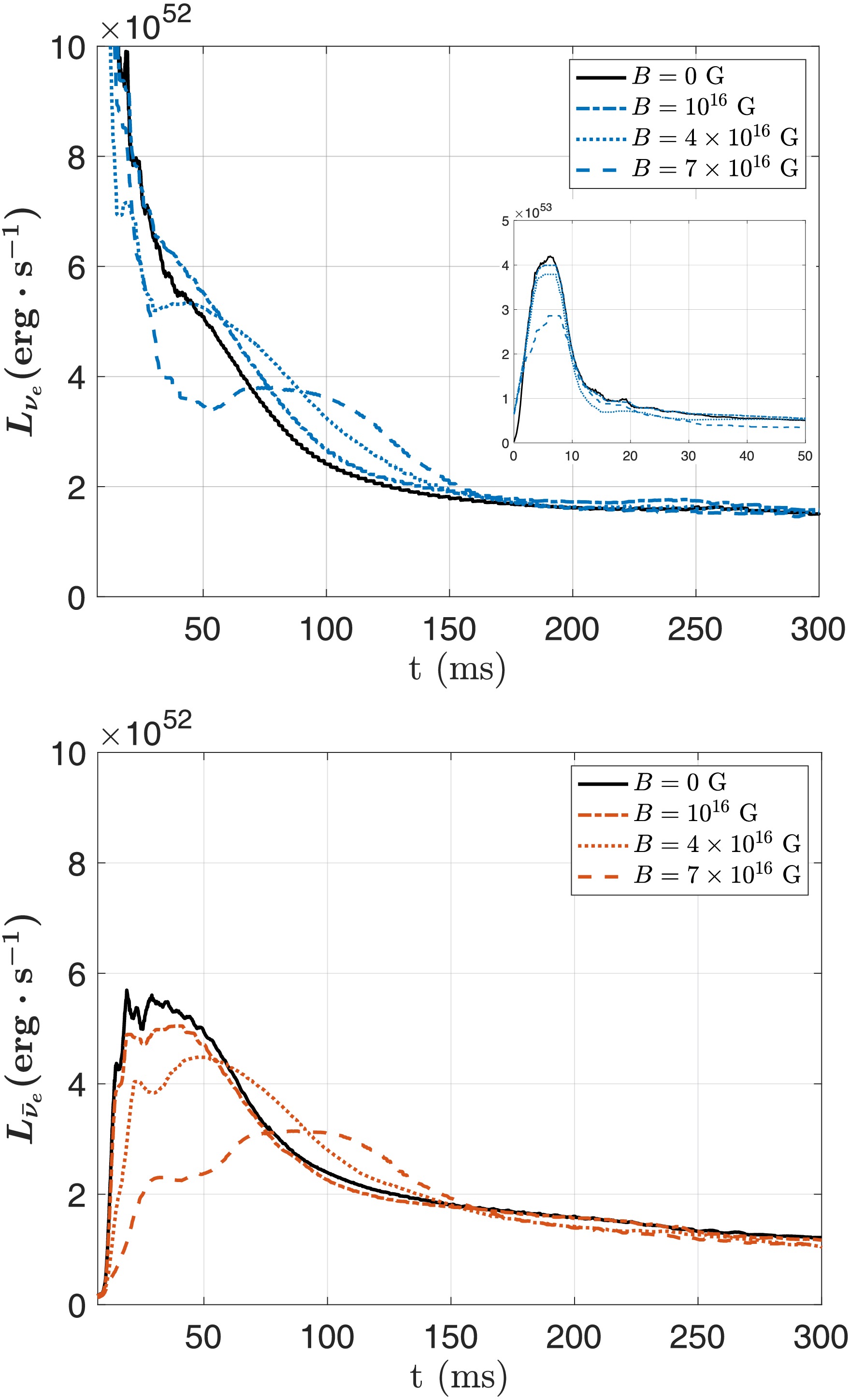
Figure 6. (color online) Upper panel: The neutrino luminosity (
$ L_{\nu_e} $ ) after core bounce. Lower panel: The antineutrino luminosity ($ L_{\bar{\nu}_e} $ ) after core bounce. The line-color convention follows Fig. 5.The situation changes after introducing the magnetic field: the peak luminosity decreases (red, green, and blue lines in each panel of Fig. 6). Especially, the
$ L_{\bar{\nu}_e} $ peak value is more sensitive to the magnetic field. This is reasonable since in each panel of Fig. 4, effective emission rates of$ \bar{\nu}_e $ show more significant changes than those of$ {\nu}_e $ . More interestingly, since the magnetic field mainly enlarges the absorption rate of neutrinos, i.e., neutrinos spend more time trapped inside the neutrinosphere, after reaching peak luminosity, both$ L_{{\nu}_e} $ and$ L_{\bar{\nu}_e} $ decay time scales become longer.Furthermore, the integrated energy of
$ \nu_e $ until 300 ms is reduced by about 10% ($ 1.13\times 10^{52} $ erg for the field-free case,$ 1.03\times 10^{52} $ erg for a$ 7\times 10^{16} $ G magnetic field). While for$ \bar{\nu}_e $ , more trapping time leads to about a 20% reduction of integrated energy ($ 6.92\times 10^{51} $ erg and$ 5.52 \times 10^{51} $ erg for the field-free and$ 7\times 10^{16} $ G cases, respectively).Fig. 7 shows the time evolution of neutrino mean energies
$ \langle E_{\nu_e}\rangle $ (upper panel) and$ \langle E_{\bar{\nu}_e}\rangle $ (lower panel) at the corresponding neutrinospheres. Because the employed leakage scheme assumes the neutrino energy spectra to be Fermi-Dirac, the neutrino mean energies are tightly correlated with the local matter temperatures. Thus, the dependence of their time evolution on the magnetic field strength reflects the corresponding dependence of the neutrinosphere evolution (see Fig. 5). With a stronger magnetic field, the neutrino mean energies are smaller shortly after the bounce and reach their peak values at later times. Note that this gray neutrino leakage scheme cannot accurately predict their energy spectra and mean values. Nevertheless, the general dependence on the magnetic field strength found here should still hold in simulations with more accurate multi-energy group neutrino transport.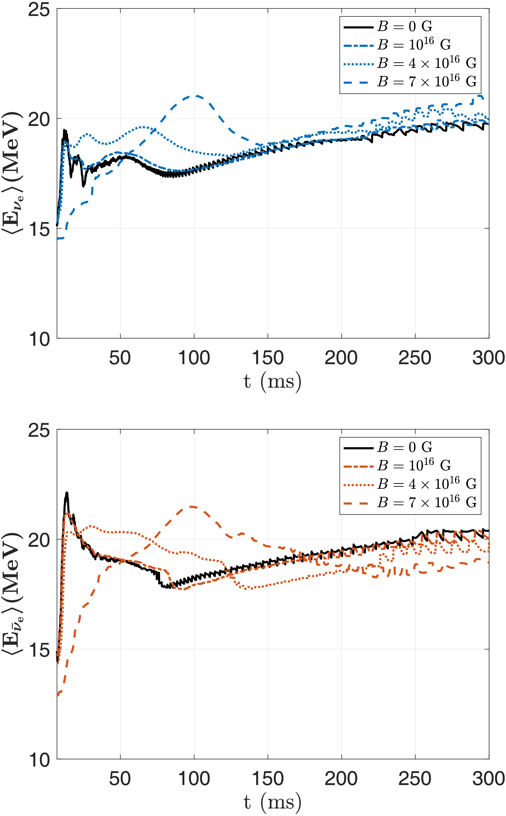
Figure 7. (color online) Upper panel: The neutrino mean energy (
$ \langle E_{\nu_e}\rangle $ ) as a function of time after the core bounce. Lower panel: The anti-neutrino mean energy ($ \langle E_{\bar{\nu}_e}\rangle $ ) as a function of time after the core bounce. The line-color convention follows Fig. 5.We further inspect the impacts of the modified neutrino transport by the magnetic field on the neutrino heating and explosion dynamics. Fig. 8 compares the evolution of the shock radius (
$ R_{\rm{sh}} $ , left y-axis) and gain radius ($ R_{\rm{g}} $ , right y-axis) between the field-free and strongest field cases. The gain radius separates the net neutrino cooling and heating regions, and its location and time evolution are crucial for the explodability of CCSNe. Before$ \sim75 $ ms post-bounce,$ R_{\rm{g}} $ is smaller by at most$ \sim20 $ km in the case of a strong magnetic field than in the field-free case. Accordingly, the runaway shock expansion takes place earlier ($ \sim60 $ ms post-bounce) in the case of a strong magnetic field than in the field-free case ($ \sim120 $ ms post-bounce). During$ \sim75-100 $ ms,$ R_{\rm{g}} $ in the case of a strong magnetic field becomes larger than in the field-free case due to the earlier runaway shock expansion. After$ \sim100 $ ms post-bounce,$ R_{\rm{g}} $ is almost identical for the two cases because it has receded to below$ \sim50 $ km where the magnetic field does not affect the neutrino opacities (cf. Fig. 2) and transport (cf. Fig. 4).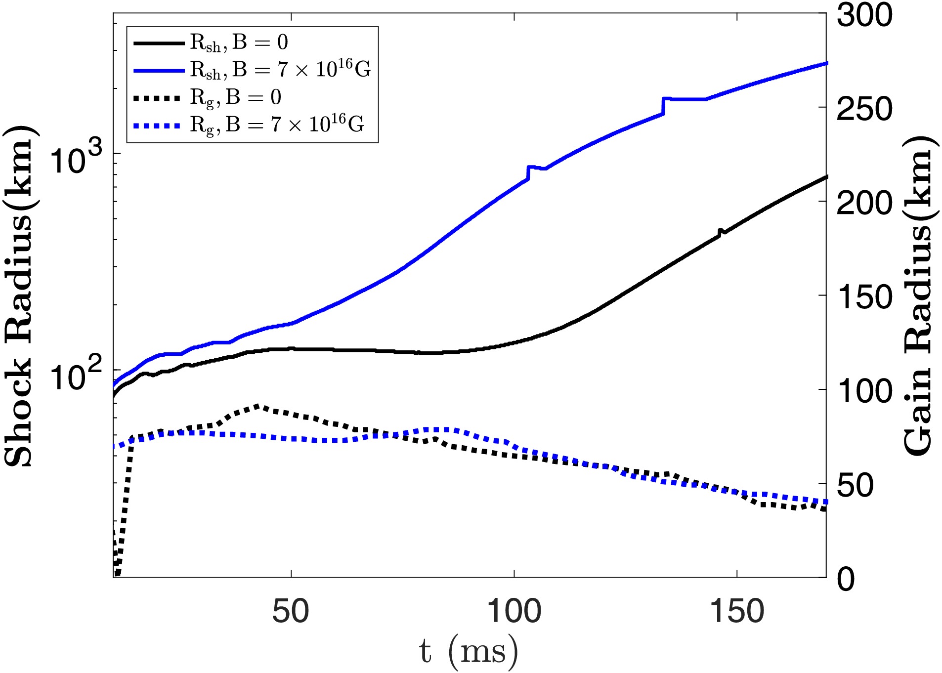
Figure 8. (color online) The comparison of shock radius
$ R_{\rm{sh}} $ (solid lines) and gain radius$ R_{\rm{g}} $ (dotted lines) under the field-free case (black lines) and$ 7\times10^{16} $ G (blue lines). The gain radius separates the net neutrino cooling (below$ R_{\rm{g}} $ ) and heating (above$ R_{\rm{g}} $ ) regions. -
We first use the extracted density, temperature, and
$ Y_e $ profiles at a certain time step from the${\tt{GR1D}} $ code to clarify the magnetic field impacts inside CCSN. Figure 2 illustrates the total opacity$ \kappa_{\rm{tot}} $ of neutrinos (blue lines, left y-axis) and antineutrinos (red lines, right y-axis) during different stages (1, 50, and 100 ms after core bounce, respectively) of CCSN. In the inner region of CCSN, neutrino scattering contributes the most to opacity, so the modification of absorption processes can be ignored.
Figure 2. (color online) The opacity of
$ \nu_e $ and$ \bar{\nu}_e $ inside CCSN is compared at different stages: 1 ms, 50 ms, and 100 ms after core bounce. Blue lines represent the opacity for$ \nu_e $ , while red lines represent the opacity for$ \bar{\nu}_e $ . The gray solid lines on all panels show the opacity contributed by scattering processes:$ \nu_e + n(p) \to \nu_e + n(p) $ and$ \bar{\nu}_e + n(p) \to \bar{\nu}_e + n(p) $ . The line styles—solid, dash-dotted, dotted, and dashed—indicate the cases for$ B = 0 $ ,$ B = 10^{16} $ G,$ B = 4\times 10^{16} $ G, and$ B = 7\times 10^{16} $ G, respectively.At a very early phase after core bounce, the shock propagates in a high-density and high-temperature region, so the magnetic field does not make significant contributions, i.e., there is no difference between each line for various magnetic field strengths (upper panel of Fig. 2). The magnetic field enhances absorption opacity when the shock propagates to
$ r \geq 30 $ km (middle and lower panel of Fig. 2). This is mainly caused by two effects: 1) The magnetic field quantizes the phase space of$ e^\pm $ , with extra magnetic energy contribution, which enhances the neutrino-nucleon interaction rates. 2) The electron chemical potential$ \mu_e $ is suppressed since only the LLL is occupied, as we discussed in Sec. II, leading to a larger value of the blocking factor$ g(E_n,-\mu_e; T_e) $ than$ g(E_n,\mu_e; T_e) $ . These impacts are consistent with those in the M1 scheme, as we discussed in [39], i.e., both the cross section deviation and chemical potential modification have a more pronounced effect on$ \bar{\nu}_e $ , leading to a greater enhancement of$ \bar{\nu}_e $ opacity compared to that of$ \nu_e $ .At a relatively later stage (
$ t\sim 100 $ ms), the matter cools down, and the magnetic field could enhance opacity by about 2−3 orders of magnitude in the region 100 km$ <r< $ 1000 km inside CCSN (lower panel of Fig. 2). However, the optical depth in such a later phase is mainly determined by the opacity of the inner region ($ r<30 $ km) due to the sharp decay of opacity with radius. Therefore, the neutrinosphere would eventually become indistinguishable from the field-free scenario.Notice that in a more realistic dipole field case, the
$ \Theta_\nu $ in Eq. (1) depends on the neutrino momentum direction and field direction. We apply different$ \Theta_\nu $ values to calculate the angle dependence of$ \kappa_{abs}(\nu_e) $ as a function of$ \eta_{\nu_e} $ . The results are shown in Fig. 3. Here, the widths of the blue and yellow bands are caused by changing the value of$ \Theta_\nu $ from 0 to π. The temperature and density are set to be$ T=1 $ MeV and$ \rho= 10^9\rm \ g\cdot cm^{-3} $ . The absorption opacity can differ by a factor of 2 by changing the value of$ \Theta_\nu $ for$ B=10^{17} $ G. However, this is the upper limit of the magnetic field strength. The yellow band shows less than a 20% difference for the case of a$ 4\times10^{16} $ G magnetic field, indicating that neglecting the angular effect can be a reasonable approximation, so we set$ \Theta_\nu=0 $ throughout this work.
Figure 3. (color online) The neutrino absorption opacity
$ \kappa_{\rm{abs}} $ is considered under varying magnetic field strengths. The black solid line represents the field-free case. The blue band corresponds to a magnetic field strength of$ 10^{17} $ G, with different values of$ \Theta_\nu $ ; the lower boundary of the band represents$ \Theta_\nu=0 $ , while the upper boundary represents$ \Theta_\nu=\pi $ . Similarly, the yellow band corresponds to a magnetic field strength of$ 4\times 10^{16} $ G, with the same interpretation for the lower and upper boundaries. In this figure, the temperature is set at$ T=1 $ MeV and the density at$ \rho= 10^9\; {\rm{g}}\cdot {\rm{cm}}^{-3} $ .The effective neutrino emission rates, as seen in Eq. (B3), describe whether the neutrinos are diffused or emitted inside a CCSN. In a high-density regime, diffusion rates are high, which governs the main neutrino number and energy loss. In contrast, the main process becomes the local emission rate if neutrinos travel to a low-density region. We show the effective emission rates in Fig. 4 for different stages of a CCSN (from top to bottom panel: 1, 50, and 100 ms after the core bounce, respectively). Again, we compare the impacts of the magnetic field under the extracted density, temperature, and
$ Y_e $ conditions in this figure. About 50 ms after core bounce (middle panel of Fig. 4), a magnetic field suppresses the effective neutrino emission rates in the range of$ 30\ {\rm{km}}< r \lt 100 \ {\rm{km}} $ , due to the enhancement of opacity shown in the middle panel of Fig. 2. Also, this result is consistent with the reduction of the diffusion rates in this region (cf. Appendix B). At 100 ms after core bounce (lower panel of Fig. 4), the shock has already propagated to the outer region, so the matter cools down and has a lower density. Diffusion is not essential in such an environment, while the local emission rates are enhanced more drastically (cf. Appendix B), leading to stronger effective emission rates.
Figure 4. (color online) The effective energy emission rate of
$ \nu_e $ and$ \bar{\nu}_e $ inside the CCSN after the core bounce. The line-color convention follows Fig. 2.We further modified the neutrino transport in
${\tt{GR1D}} $ based on Eq. (9), Eq. (10), and equations in Appendix B to perform 1-D simulations with a magnetic field. We investigate the impacts of a constant magnetic field in a region$ r<r_{\rm{cut}}=100 $ km in our CCSN simulation. The enhanced opacity enlarges the radius of the neutrinosphere, which is shown in Fig. 5, where the time evolution of the neutrinosphere for$ \nu_e $ and$ \bar{\nu}_e $ are shown in the upper and lower panels, respectively (our calculation uses the opacity for neutrino-energy transport$ \kappa_{{\rm{tot}},1}(\nu_i) $ to determine the neutrinosphere). The radius of the neutrinosphere is indistinguishable under different magnetic field cases at$ t<10 $ ms after core bounce. After a few dozen milliseconds, when the shock propagates outside the high-density and high-temperature region,$ \kappa_{\rm{tot}} $ increases, and one can see the enlargement of the neutrinosphere as expected. Usually, without a magnetic field, the radius of the neutrinosphere is larger than that of anti-neutrinos. This is because the proton abundance reduces after the shock passage, leading to a smaller value of the absorption opacity$ \kappa_{a} $ . However, for a magnetic field as strong as$ 7\times 10^{16} $ G (i.e., blue lines),$ R_{\bar{\nu}_e} $ becomes comparable with$ R_{\nu_e} $ , which is consistent with the fact that the magnetic field enlarges$ \kappa_{a}(\bar{\nu}_e) $ more than$ \kappa_{a}({\nu}_e) $ as we discussed above. The effective emission rates further determine neutrino luminosity, as shown in Fig. 6. After core bounce,$ \nu_e $ is created by the electron capture on protons in the heated matter. A luminous flash of neutronization$ \nu_e $ is radiated when the shock travels to the low-density region outside the neutrinosphere. In the field-free case,$ L_{\nu_e} $ reaches a peak value near$ 4\times 10^{53} \;{\rm{erg}}\cdot {\rm{s}}^{-1} $ at$ \sim 7 $ ms (black solid line of the upper panel, also see the inset figure on the upper panel). The peak of$ L_{\bar{\nu}_e} $ occurs shortly after the neutrinos (black solid line of the lower panel), with a value of about$ 6\times 10^{52} \rm \ erg\cdot s^{-1} $ at$ \sim 30 $ ms; this is due to$ \bar{\nu}_e $ production by pair processes in shock-heated matter at a later time.
Figure 5. (color online) Upper panel: The neutrinosphere evolution (
$ \nu_e $ ) after core bounce. Lower panel: The neutrinosphere evolution of$ \bar{\nu}_e $ after core bounce. Black solid lines correspond to the field-free case; red, green, and blue lines correspond to$ B=10^{16} $ G,$ B=4\times 10^{16} $ G, and$ B=7\times 10^{16} $ G, respectively.
Figure 6. (color online) Upper panel: The neutrino luminosity (
$ L_{\nu_e} $ ) after core bounce. Lower panel: The antineutrino luminosity ($ L_{\bar{\nu}_e} $ ) after core bounce. The line-color convention follows Fig. 5.The situation changes after introducing the magnetic field: the peak luminosity decreases (red, green, and blue lines in each panel of Fig. 6). Especially, the
$ L_{\bar{\nu}_e} $ peak value is more sensitive to the magnetic field. This is reasonable since in each panel of Fig. 4, effective emission rates of$ \bar{\nu}_e $ show more significant changes than those of$ {\nu}_e $ . More interestingly, since the magnetic field mainly enlarges the absorption rate of neutrinos, i.e., neutrinos spend more time trapped inside the neutrinosphere, after reaching peak luminosity, both$ L_{{\nu}_e} $ and$ L_{\bar{\nu}_e} $ decay time scales become longer.Furthermore, the integrated energy of
$ \nu_e $ until 300 ms is reduced by about 10% ($ 1.13\times 10^{52} $ erg for the field-free case,$ 1.03\times 10^{52} $ erg for a$ 7\times 10^{16} $ G magnetic field). While for$ \bar{\nu}_e $ , more trapping time leads to about a 20% reduction of integrated energy ($ 6.92\times 10^{51} $ erg and$ 5.52 \times 10^{51} $ erg for the field-free and$ 7\times 10^{16} $ G cases, respectively).Figure 7 shows the time evolution of neutrino mean energies
$ \langle E_{\nu_e}\rangle $ (upper panel) and$ \langle E_{\bar{\nu}_e}\rangle $ (lower panel) at the corresponding neutrinospheres. Because the employed leakage scheme assumes the neutrino energy spectra to be Fermi-Dirac, the neutrino mean energies are tightly correlated with the local matter temperatures. Thus, the dependence of their time evolution on the magnetic field strength reflects the corresponding dependence of the neutrinosphere evolution (see Fig. 5). With a stronger magnetic field, the neutrino mean energies are smaller shortly after the bounce and reach their peak values at later times. Note that this gray neutrino leakage scheme cannot accurately predict their energy spectra and mean values. Nevertheless, the general dependence on the magnetic field strength found here should still hold in simulations with more accurate multi-energy group neutrino transport.
Figure 7. (color online) Upper panel: The neutrino mean energy (
$ \langle E_{\nu_e}\rangle $ ) as a function of time after the core bounce. Lower panel: The anti-neutrino mean energy ($ \langle E_{\bar{\nu}_e}\rangle $ ) as a function of time after the core bounce. The line-color convention follows Fig. 5.We further inspect the impacts of the modified neutrino transport by the magnetic field on the neutrino heating and explosion dynamics. Figure 8 compares the evolution of the shock radius (
$ R_{\rm{sh}} $ , left y-axis) and gain radius ($ R_{\rm{g}} $ , right y-axis) between the field-free and strongest field cases. The gain radius separates the net neutrino cooling and heating regions, and its location and time evolution are crucial for the explodability of CCSNe. Before$ \sim75 $ ms post-bounce,$ R_{\rm{g}} $ is smaller by at most$ \sim20 $ km in the case of a strong magnetic field than in the field-free case. Accordingly, the runaway shock expansion takes place earlier ($ \sim60 $ ms post-bounce) in the case of a strong magnetic field than in the field-free case ($ \sim120 $ ms post-bounce). During$ \sim75-100 $ ms,$ R_{\rm{g}} $ in the case of a strong magnetic field becomes larger than in the field-free case due to the earlier runaway shock expansion. After$ \sim100 $ ms post-bounce,$ R_{\rm{g}} $ is almost identical for the two cases because it has receded to below$ \sim50 $ km where the magnetic field does not affect the neutrino opacities (cf. Fig. 2) and transport (cf. Fig. 4).
Figure 8. (color online) The comparison of shock radius
$ R_{\rm{sh}} $ (solid lines) and gain radius$ R_{\rm{g}} $ (dotted lines) under the field-free case (black lines) and$ 7\times10^{16} $ G (blue lines). The gain radius separates the net neutrino cooling (below$ R_{\rm{g}} $ ) and heating (above$ R_{\rm{g}} $ ) regions. -
In this study, we derived the neutrino leakage scheme formula under the influence of strong magnetic fields and employed the
${\tt{GR1D}} $ code to perform a 1-D CCSN simulation of a 9.6 M⊙ zero-metallicity progenitor. The presence of a magnetic field modifies the neutrino absorption cross sections and diminishes the$ e^\pm $ chemical potential, as these particles are restricted to the lowest Landau level. We studied the effects of a constant magnetic field within a specific radius configuration, assuming field strengths ranging from$ 10^{16} $ G to$ 7 \times 10^{16} $ G during the post-bounce phase.The magnetic field enhances the absorption rates of neutrinos and antineutrinos, enlarging their opacities (Fig. 2). This is consistent with results from the M1 scheme, where both cross section deviations and chemical potential modifications have more pronounced effects on
$ \bar{\nu}_e $ , leading to a greater enhancement of$ \bar{\nu}_e $ opacity compared to$ \nu_e $ . The larger opacity increases the trapping timescale of neutrinos inside the neutrinosphere, resulting in longer decay timescales for neutrino luminosities and smaller peak luminosities (Fig. 6). Accordingly, with stronger magnetic fields, neutrinos exhibit lower mean energies shortly after bounce and reach their peak values at later times (Fig. 7).These results demonstrate that the leakage scheme provides an efficient and practical framework for studying the qualitative impacts of magnetic fields on neutrino transport in 1D CCSNe simulations.
-
In Eqs. 9 and 10,
$ Y_{\rm{np}} $ and$ Y_{\rm{pn}} $ are given by [9, 10]:$ \begin{aligned} Y_{\rm{np}} = \dfrac{2Y_e -1 }{ \exp{(\eta_p-\eta_n)}-1}; Y_{ \rm pn} = \exp{(\eta_p-\eta_n)} \cdot Y_{\rm{np}}, \end{aligned} $
(A1) Where
$ \eta_{n(p)} = \mu_{n(p)}/k_BT $ is the degeneracy parameter of protons and neutrons. The neutrino degeneracy parameters$ \eta_\nu $ are determined from the local optical depth$ \tau_{\nu_i}(r) $ :$ \begin{aligned} \left\{ \begin{aligned} &\eta_{\nu_x}(r) = 0\ \ \ \ \ \ \\ &\eta_{\nu_e}(r) = \eta^{eq}_{\nu_e} \cdot \big[1-\exp{(-\tau_{\nu_e}(r))}\big] \ \ \ \ \ \ \ \\ &\eta_{\bar{\nu}_e}(r) = - \eta^{eq}_{\bar{\nu}_e} \cdot \big[1-\exp{(-\tau_{\bar{\nu}_e}(r))}\big]. \end{aligned} \right. \end{aligned} $
(A2) Here,
$ \eta^{eq} $ is the degeneracy parameter in the equilibrium state, following the relation:$ \begin{aligned} \eta^{eq}_{\nu_e} = -\eta^{eq}_{\bar{\nu}_e} = \eta_e(B) +\eta_p - \eta_n -Q/k_BT, \end{aligned} $
(A3) where
$ Q = m_n-m_p $ . -
In Eqs. (9) and (10),
$ Y_{np} $ and$ Y_{pn} $ are given by [9, 10]:$ \begin{aligned} Y_{np} = \dfrac{2Y_e -1 }{ \exp{(\eta_p-\eta_n)}-1}; Y_{ pn} = \exp{(\eta_p-\eta_n)} \cdot Y_{np}, \end{aligned} $
(A1) where
$ \eta_{n(p)} = \mu_{n(p)}/k_BT $ is the degeneracy parameter of protons and neutrons. The neutrino degeneracy parameters$ \eta_\nu $ are determined from the local optical depth$ \tau_{\nu_i}(r) $ :$ \begin{aligned} \left\{ \begin{aligned} &\eta_{\nu_x}(r) = 0\ \ \ \ \ \ \\ &\eta_{\nu_e}(r) = \eta^{eq}_{\nu_e} \cdot \big[1-\exp{(-\tau_{\nu_e}(r))}\big] \ \ \ \ \ \ \ \\ &\eta_{\bar{\nu}_e}(r) = - \eta^{eq}_{\bar{\nu}_e} \cdot \big[1-\exp{(-\tau_{\bar{\nu}_e}(r))}\big]. \end{aligned} \right. \end{aligned} $
(A2) Here,
$ \eta^{eq} $ is the degeneracy parameter in the equilibrium state, following the relation:$ \begin{aligned} \eta^{eq}_{\nu_e} = -\eta^{eq}_{\bar{\nu}_e} = \eta_e(B) +\eta_p - \eta_n -Q/k_BT, \end{aligned} $
(A3) where
$ Q = m_n-m_p $ . -
Under a magnetic field, local emission rates from
$ e^\pm $ capture are given by$ \begin{aligned} &R^B_{e,j}(e^- p) = A\rho Y_{\rm{np}}\times\\ &\int_0^\infty dE_{\nu_e} \sigma(E_n,B)E_{\nu_e}^{2+j} g(E_{\nu_e}, \eta_{\nu_e}; T_{\nu_e})f_{\rm{FD}}\Big[E_n, \mu_e(B);T_e\Big], \end{aligned} $
(B1) $ \begin{aligned} &R^B_{e,j}(e^+ n) = A\rho Y_{\rm{pn}} \times\\ &\int_0^\infty dE_{\bar{\nu}_e}\sigma(E_n,B)E_{\bar{\nu}_e}^{2+j} g(E_{\bar{\nu}_e}, \eta_{\bar{\nu}_e}; T_{\bar{\nu}_e}) f_{\rm{FD}}\Big[E_n, -\mu_e(B);T_{e}\Big], \nonumber \end{aligned} $
(B2) where
$ j=0 $ is the number emission rate, and$ j=1 $ is the energy emission rate. Pair creation ($ e^- + e^+ \to \nu_e + \bar{\nu}_e $ ) and the Bremsstrahlung effect are also included in the${\tt{GR1D}} $ code. We consider these two types of$ \nu_e (\bar{\nu}_e) $ emission rates as field-free scenarios. Similar to [9, 10], this work uses the effective emission rates in the leakage scheme:$ \begin{aligned} R_{\rm{eff}} =\dfrac{ R_{\rm{emit}} }{ 1+R_{\rm{emit}}/R_{\rm{diff}}},\ Q_{\rm{eff}} =\dfrac{ Q_{\rm{emit}} }{ 1+Q_{\rm{emit}}/Q_{\rm{diff}}}, \end{aligned} $
(B3) where
$ R_{\rm{emit}} $ and$ Q_{\rm{emit}} $ represent the local neutrino number and energy emission rates, respectively:$ \begin{aligned}[b]& R_{\rm{emit}} = R^B_{e,0}+R_{\rm{Pair}}+R_{\rm{Brem}}, \\& Q_{\rm{emit}} = R^B_{e,1}+Q_{\rm{Pair}}+Q_{\rm{Brem}}. \end{aligned} $
(B4) The local diffusion rates,
$ R_{\rm{diff}} $ and$ Q_{\rm{diff}} $ , are calculated following the approximation made in [9]:$ \begin{aligned} R_{\rm{diff}} = \dfrac{4\pi c g_{\nu_i}}{ (hc)^3}\dfrac{\zeta_{\nu_i}}{ 3\chi^2_{\nu_i}}TF_0(\eta_{\nu_i}), \end{aligned} $
(B5) $ \begin{aligned} Q_{\rm{diff}} = \dfrac{4\pi c g_{\nu_i}}{ (hc)^3}\dfrac{\zeta_{\nu_i}}{ 3\chi^2_{\nu_i}}T^2F_1(\eta_{\nu_i}), \end{aligned} $
(B6) for neutrino species
$ \nu_i $ , where$ \chi_{\nu_i}=\int \zeta_{\nu_i} dr $ . The strong magnetic field changes the neutrino absorption rate on nucleons, i.e., the values of$ \zeta_{\nu_e}({\nu}_e n) $ and$ \zeta_{\bar{\nu}_e}(\bar{\nu}_e p) $ are modified. By definition, these two quantities are the local absorption rates over$ \langle E^2 \rangle $ when calculating the diffusion rate:$ \begin{aligned}[b] \zeta_{\nu_e}({\nu}_e n) =\;& A\rho Y_{\rm{np}} \\ &\times\dfrac{\int_0^\infty \sigma(E_n, B)E_{\nu_e}^{2} f_{\rm{FD}}(E_{\nu_e}, \eta_{\nu_e}; T_{\nu_e}) g\Big[E_n, \mu_e(B);T_e\Big] }{ \int_0^\infty E_\nu^{4} f_{\rm{FD}}(E_{\nu_e}, \eta_{\nu_e}; T_{\nu_e})}, \end{aligned} $
(B7) $ \begin{aligned}[b] \zeta_{\bar{\nu}_e}(\bar{\nu}_e p)=\;& A\rho Y_{\rm{np}} \\ &\times\dfrac{\int_0^\infty \sigma(E_n, B)E_{\bar{\nu}_e}^{2} f_{\rm{FD}}(E_{\bar{\nu}_e}, \eta_{\bar{\nu}_e}; T_\nu) g\Big[E_n, - \mu_e(B);T_{e}\Big] }{ \int_0^\infty E_{\bar{\nu}_e}^{4} f_{\rm{FD}}(E_{\bar{\nu}_e}, \eta_{\bar{\nu}_e}; T_{\bar{\nu}_e})}. \end{aligned} $
(B8) Figure B1 illustrates the local diffusion rate of neutrinos.
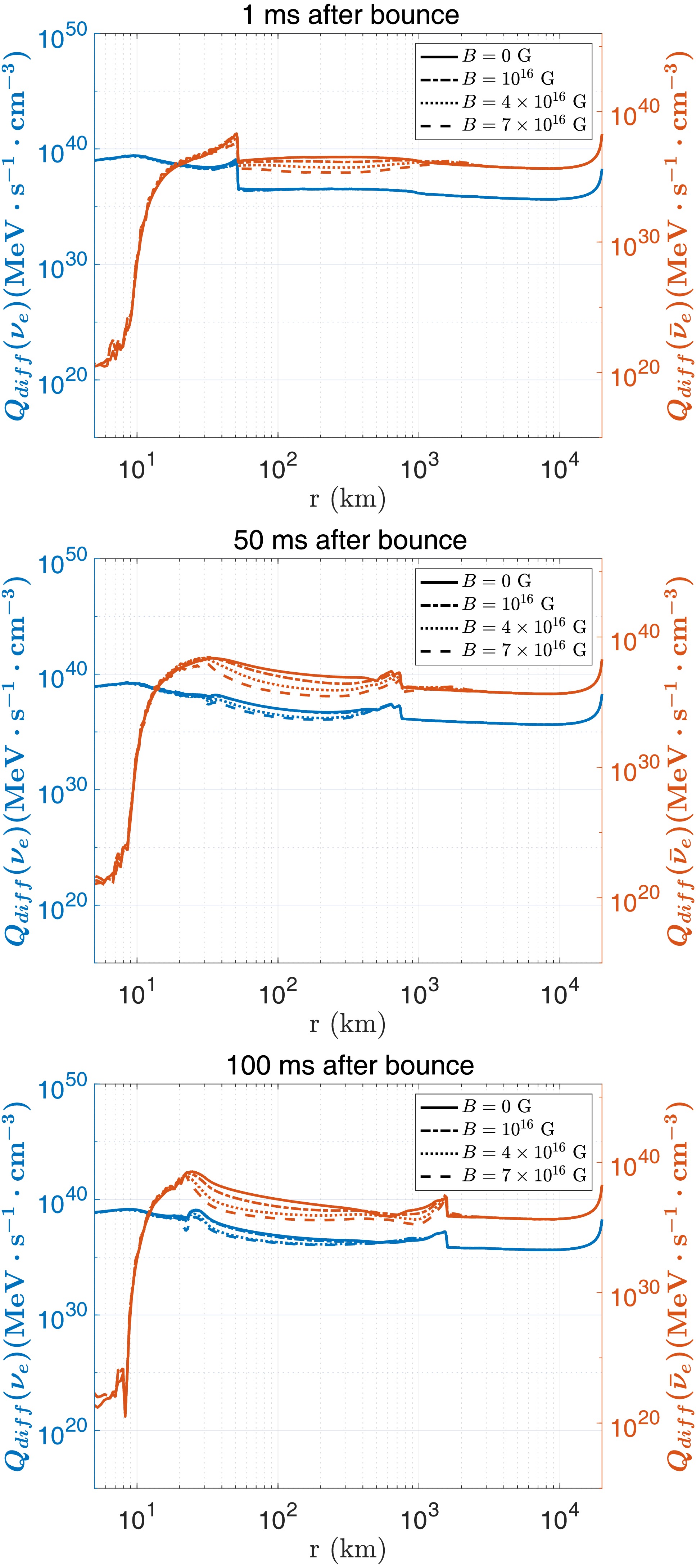
Figure B1. (color online) The diffusion rates of
$ \nu_e $ and$ \bar{\nu}_e $ inside the CCSN at different bouncing phases (1 ms, 50 ms, and 100 ms, respectively) are presented. The blue lines indicate the emission rate for$ \nu_e $ , and the red lines represent$ \bar{\nu}_e $ . The results for the cases where$ B = 0 $ ,$ B = 10^{16} $ G,$ B = 5\times 10^{16} $ G, and$ B= 10^{17} $ G are shown in solid, dash-dotted, dotted, and dashed lines, respectively.Figure B2 compares the local emission rate during different phases of CCSN.
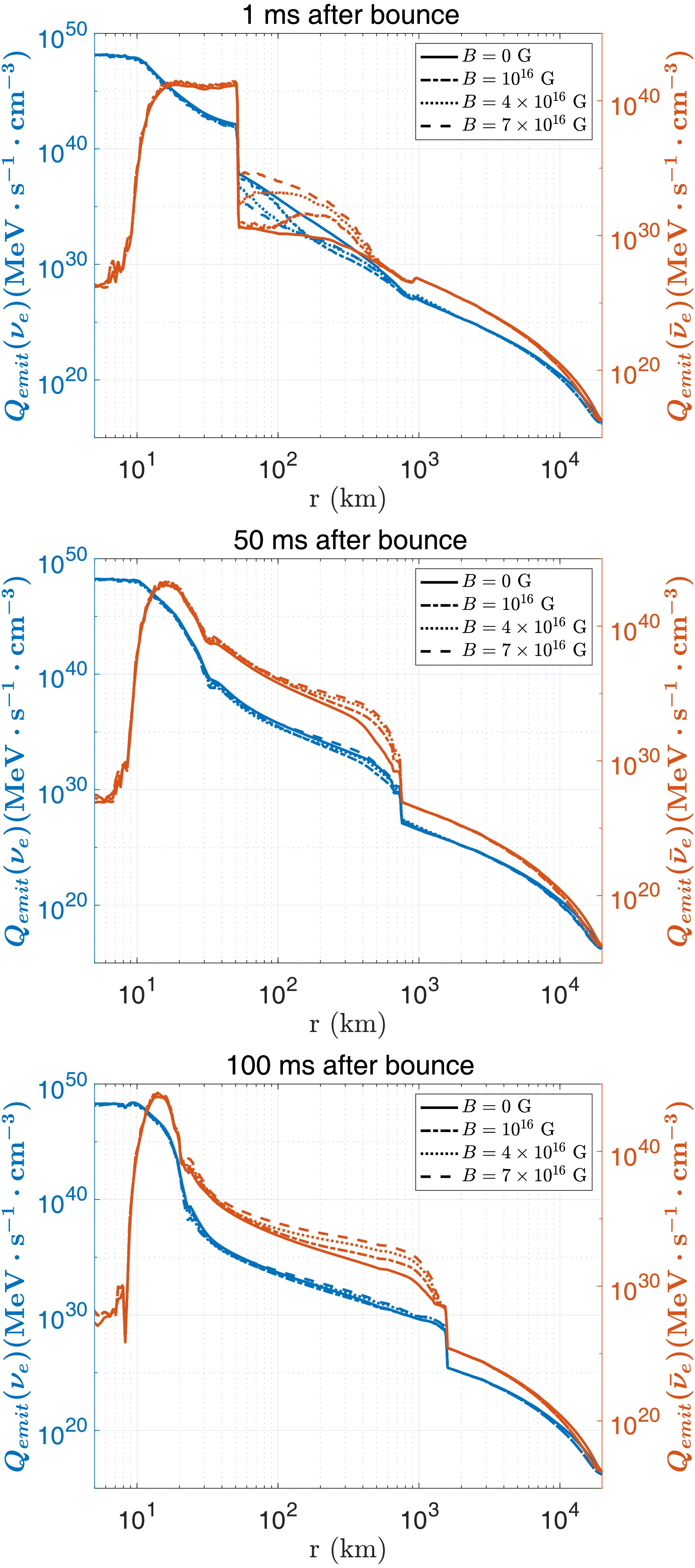
Figure B2. (color online) The emission rate of
$ \nu_e $ and$ \bar{\nu}_e $ inside the CCSN is examined at different bounce phases. The line-color convention follows Fig. B1. -
Under a magnetic field, local emission rates from
$ e^\pm $ capture are given by$ \begin{aligned} &R^B_{e,j}(e^- p) = A\rho Y_{{np}}\\ &\times\int_0^\infty {\mathrm{d}}E_{\nu_e} \sigma(E_n,B)E_{\nu_e}^{2+j} g(E_{\nu_e}, \eta_{\nu_e}; T_{\nu_e})f_{\rm{FD}}\Big[E_n, \mu_e(B);T_e\Big], \end{aligned} $
(B1) $ \begin{aligned} &R^B_{e,j}(e^+ n) = A\rho Y_{{pn}}\\ & \times\int_0^\infty {\mathrm{d}}E_{\bar{\nu}_e}\sigma(E_n,B)E_{\bar{\nu}_e}^{2+j} g(E_{\bar{\nu}_e}, \eta_{\bar{\nu}_e}; T_{\bar{\nu}_e}) f_{\rm{FD}}\Big[E_n, -\mu_e(B);T_{e}\Big], \nonumber \end{aligned} $
(B2) where
$ j=0 $ is the number emission rate, and$ j=1 $ is the energy emission rate. Pair creation ($ e^- + e^+ \to \nu_e + \bar{\nu}_e $ ) and the Bremsstrahlung effect are also included in the${\tt{GR1D}} $ code. We consider these two types of$ \nu_e (\bar{\nu}_e) $ emission rates as field-free scenarios. Similar to [9, 10], this work uses the effective emission rates in the leakage scheme:$ \begin{aligned} R_{\rm{eff}} =\dfrac{ R_{\rm{emit}} }{ 1+R_{\rm{emit}}/R_{\rm{diff}}},\ Q_{\rm{eff}} =\dfrac{ Q_{\rm{emit}} }{ 1+Q_{\rm{emit}}/Q_{\rm{diff}}}, \end{aligned} $
(B3) where
$ R_{\rm{emit}} $ and$ Q_{\rm{emit}} $ represent the local neutrino number and energy emission rates, respectively:$ \begin{aligned}[b]& R_{\rm{emit}} = R^B_{e,0}+R_{\rm{Pair}}+R_{\rm{Brem}}, \\& Q_{\rm{emit}} = R^B_{e,1}+Q_{\rm{Pair}}+Q_{\rm{Brem}}. \end{aligned} $
(B4) The local diffusion rates,
$ R_{\rm{diff}} $ and$ Q_{\rm{diff}} $ , are calculated following the approximation made in [9]:$ \begin{aligned} R_{\rm{diff}} = \dfrac{4\pi c g_{\nu_i}}{ (hc)^3}\dfrac{\zeta_{\nu_i}}{ 3\chi^2_{\nu_i}}TF_0(\eta_{\nu_i}), \end{aligned} $
(B5) $ \begin{aligned} Q_{\rm{diff}} = \dfrac{4\pi c g_{\nu_i}}{ (hc)^3}\dfrac{\zeta_{\nu_i}}{ 3\chi^2_{\nu_i}}T^2F_1(\eta_{\nu_i}), \end{aligned} $
(B6) for neutrino species
$ \nu_i $ , where$ \chi_{\nu_i}=\int_{ }^{ }\zeta_{\nu_i}\mathrm{d}r $ . The local diffusion rate and emission rate are showing in Figure B1 and B2, respectively. The strong magnetic field changes the neutrino absorption rate on nucleons, i.e., the values of$ \zeta_{\nu_e}({\nu}_e n) $ and$ \zeta_{\bar{\nu}_e}(\bar{\nu}_e p) $ are modified. By definition, these two quantities are the local absorption rates over$ \langle E^2 \rangle $ when calculating the diffusion rate:
Figure B1. (color online) The diffusion rates of
$ \nu_e $ and$ \bar{\nu}_e $ inside the CCSN at different bouncing phases (1, 50, and 100 ms, respectively) are presented. The blue lines indicate the emission rate for$ \nu_e $ , and the red lines represent$ \bar{\nu}_e $ . The results for the cases where$ B = 0 $ ,$ B = 10^{16} $ G,$ B = 5\times 10^{16} $ G, and$ B= 10^{17} $ G are shown in solid, dash-dotted, dotted, and dashed lines, respectively.
Figure B2. (color online) The emission rate of
$ \nu_e $ and$ \bar{\nu}_e $ inside the CCSN is examined at different bounce phases. The line-color convention follows Fig. B1.$ \begin{aligned}[b] \zeta_{\nu_e}({\nu}_e n) = \, & A\rho Y_{np} \\ & \times\dfrac{\displaystyle\int_0^\infty \sigma(E_n, B)E_{\nu_e}^{2} f_{\rm{FD}}(E_{\nu_e}, \eta_{\nu_e}; T_{\nu_e}) g\Big[E_n, \mu_e(B);T_e\Big] }{\displaystyle \int_0^\infty E_\nu^{4} f_{\rm{FD}}(E_{\nu_e}, \eta_{\nu_e}; T_{\nu_e})}, \end{aligned} $
(B7) $ \begin{aligned}[b] \zeta_{\bar{\nu}_e}(\bar{\nu}_e p)=\,& A\rho Y_{np} \\ &\times\dfrac{\displaystyle\int_0^\infty \sigma(E_n, B)E_{\bar{\nu}_e}^{2} f_{\rm{FD}}(E_{\bar{\nu}_e}, \eta_{\bar{\nu}_e}; T_\nu) g\Big[E_n, - \mu_e(B);T_{e}\Big] }{\displaystyle\int_0^\infty E_{\bar{\nu}_e}^{4} f_{\rm{FD}}(E_{\bar{\nu}_e}, \eta_{\bar{\nu}_e}; T_{\bar{\nu}_e})}. \end{aligned} $
(B8)
Strong magnetic field inside degenerate relativistic plasma and the impacts on the neutrino transport in Core-Collapse Supernovae
- Received Date: 2026-02-12
- Available Online: 2026-08-15
Abstract: We investigate the impacts of strong magnetic fields on neutrino transport in core-collapse supernovae (CCSNe) using the leakage scheme. The magnetic field quantizes the momentum of electrons and positrons, resulting in the modification of weak-interaction cross sections and the chemical potentials of electrons and positrons. We derive a formula for the neutrino leakage scheme, including these two impacts, and perform 1D CCSN simulations with $ {\tt{GR1D}}$. Magnetic field strengths from $ 10^{16} $ G to $ 10^{17} $ G were applied during the postbounce phase. The results show that neutrino opacities are enhanced due to the amplified interaction rates, with stronger effects on antineutrinos. This leads to larger neutrinosphere radii, longer neutrino trapping timescales, reduced peak luminosities, and delayed peak energies.


 DownLoad: