


 Abstract
 HTML
HTML Reference
 Related
 PDF
PDF


-
The Standard Model (SM) has achieved remarkable success in describing the fundamental particles and their interactions both theoretically and experimentally. Nevertheless, the search for physics beyond the SM, also known as the new physics (NP) remains one of the primary objectives of contemporary particle physics. While high-energy experiments aim to reveal new particles through direct production, precision studies provide an alternative and complementary approach for uncovering possible deviations from SM predictions. In this context, heavy-flavor physics offers a powerful laboratory for testing the SM with high accuracy, owing to the large amount of available experimental data. A central aspect of these studies is the examination of the unitarity of the Cabibbo-Kobayashi-Maskawa (CKM) matrix, where the B-meson decays are always at the forefront.
Among the various B-meson decay channels, particularly sensitive probes of the SM arise from flavor-changing neutral-current (FCNC) transitions of the type
$ b \to s(d)\ell^{+}\ell^{-} $ . In the Standard Model, these processes occur only at the loop level and are further suppressed by the CKM matrix elements. Consequently, the corresponding exclusive decay modes, such as$ B^{\pm}\to K^{(*)\pm}\ell^{+}\ell^{-} $ ,$ B^{0}\to K^{0}\ell^{+}\ell^{-} $ , and$ B_s^{0} \to \phi\,\ell^{+}\ell^{-} $ , with$ \ell=e,\mu $ , have been extensively investigated experimentally [1−7]. Of particular interest are tests of lepton-flavor universality (LFU) in$ B\to K^{(*)}\ell^{+}\ell^{-} $ decays [8−11]. In these observables, the dependence on CKM matrix elements as well as the uncertainties associated with hadronic form factors largely cancel, making them especially clean probes of possible new physics effects. As a result, these processes have been widely studied in a variety of new-physics scenarios; see, for example, Refs. [12−17]. Recent experimental measurements indicate that these observables are consistent with the SM predictions within approximately$ 0.2\sigma $ [18−21]. Motivated by these developments, it is worthwhile to explore other complementary exclusive decays induced by the same FCNC transition$ b \to s\ell^{+}\ell^{-} $ . In this context, the rare decays$ B \to S\,\ell^{+}\ell^{-} $ , where$ S=(f_0,a_0,K_0^{*}) $ denotes a scalar meson, provide an additional probe of the underlying flavor dynamics.The study of light scalar mesons with masses below
$ 1.5 $ GeV serves as an intriguing subject of study due to their non trivial internal structure. While they are usually viewed as conventional quarks-antiquark states [22], alternate descriptions have been proposed depending upon their masses and observed properties. These include tetra-quark configurations [23], meson-meson molecular states [24], and less convincingly, glueball states [25]. Although some of these models are quite successful in explaining certain experimental features, none of them provides a full experimentally observed consistent description. As a consequence, the internal structure of light scalar mesons remains an open question and continues to attract considerable interest in hadron physics. The meson$ K_0^{*}(1430) $ , which constitutes the main focus of the present study, is commonly interpreted as a predominantly$ s\bar{q} $ or$ q\bar{s} $ state in many phenomenological analyses. However, its classification is still subject to debate, with two commonly discussed scenarios in the literature. In the first scenario,$ K_0^{*}(1430) $ is treated as an excited state associated with a lighter scalar ground state below$ 1\,{\rm{GeV}} $ . In the second scenario, it is regarded as the lowest-lying scalar state, while the light scalar nonet below$ 1\,{\rm{GeV}} $ is interpreted as a set of tetraquark bound states. A detailed discussion of these possibilities can be found in Refs. [26, 27]. To probe the quark-antiquark structure of$ K_0^{*}(1430) $ , the semileptonic weak decay$ B \to K_0^{*}(1430)\ell^+\ell^- $ provides a relatively clean channel compared to purely hadronic decay modes, reducing uncertainties associated with strong interactions. As a weak decay, the key inputs to the SM calculation are the hadronic matrix elements of the weak currents, parameterised by form factors. The form factors are functions of the four-momentum transfer, q, between B and$ K_0^{*}\left(1430\right) $ and depend on the strong interaction effects that bind the quarks inside the mesons, and hence clarify the internal structure of the$ K_0^{*}\left(1430\right) $ meson. Several theoretical approaches are used in literature including simple quark model [28], light front approach [29−31], QCD sum rules [32, 33], light cone sum rules [34−36] and perturbative QCD factorization approach [37−39] for the precise measurements of these form factors.As the form factors are non-perturbative, model-dependent quantities that dominate theoretical uncertainties in B-meson decay predictions [40−45], particularly in the low momentum-transfer region. Effective field theories (EFT) allow certain symmetries to reduce the number of independent form factors. In particular, heavy-quark symmetry (HQS), applicable for mesons containing a heavy quark, provides symmetry relations [46−52] that are not explicit in full QCD. These relations allow form factors to be expressed in terms of a reduced set of universal Isgur–Wise functions, minimizing the number of hadronic parameters.
Although the form-factor structures for
$ B\to K^{*} $ [53, 54] and$ B\to D^{*} $ [40, 51, 52, 55] have been studied extensively; further efforts are continued to achieve higher precision, particularly in the kinematical situations where the outgoing degree of freedom carries a large amount of energy$ (E) $ . In such large recoil regimes relevant to semi-leptonic decays B to$ (\pi,\rho, K^{*})\ell^+\ell^- $ , the large-energy-effective-theory (LEET) plays an important role by providing an essential theoretical framework. Within this approach, form factors can be factorized using HQS, for the initial state heavy meson and LEET for energetic final state light meson, into hard and soft parts [56−58]. The soft contributions correspond to gluon interactions of order$ \Lambda_Q{}_C{}_D/m_b $ while the hard spectator part, involving the spectator quark, is of order$ m_b\Lambda_Q{}_C{}_D $ . In the decay$ B\to V $ , LEET reduces the seven form factors into two in the large recoil limit. Furthermore, the large-energy of the final state meson further highlights the importance of perturbative corrections. To compute these corrections, one needs a suitable factorization scheme to separate the perturbative and the non-perturbative parts. One such factorization scheme is introduced in Eq.(23). In this framework, the hard gluon vertex corrections are absorbed in the coefficients$ C_i $ of the soft-form factors. Additionally, at order$ 1/m_b $ , all end-point singularities [59] that appear in the hard-spectator interactions are also absorbed in the soft-form factors as they respect heavy quark symmetry. On the other hand, the corrections that violate these symmetries are treated separately and explicitly incorporated in the form factors.The main objective of this study is the calculation of hard-spectator corrections together with vertex renormalization for the decay
$ B \to K_0^{*}(1430)\,\ell^+\ell^- $ . In the large-energy limit, heavy-quark symmetry reduces the three form factors defined through the relevant matrix elements to a single universal function,$ \xi_{K_0^{*}}(E_F) $ . Symmetry-breaking corrections to this form factor are evaluated explicitly using vertex renormalization and hard-spectator interactions. An accurate determination of these corrections is essential not only for reliable theoretical predictions but also for guiding future high-precision measurements at experiments such as LHCb and Belle II, where rare semileptonic B-meson decays provide sensitive probes of hadronic dynamics and potential new-physics effects. After quantifying these corrections, we analyze their impact on physical observables, including the branching ratio and various lepton-polarization asymmetries in these decays.This work is organized as follows: In the Sec. II, we have discussed the theoretical framework used to evaluate the form factors under the symmetry relation. Sec. III is divided into two parts: the first part discusses the correction to the vertex, while the second portion is dedicated to hard spectator correction at order
$ \alpha_s $ using the light cone distribution amplitudes (LCDAs). These form factors serve as important inputs for the analysis of the branching fraction and lepton polarization asymmetry. Our numerical and analytical results and their comparison with the theoretical predictions are presented in Sec. IV. Finally, Sec. V is dedicated to the conclusion. -
The Standard Model (SM) has achieved remarkable success in describing the fundamental particles and their interactions both theoretically and experimentally. Nevertheless, the search for physics beyond the SM, also known as the new physics (NP) remains one of the primary objectives of contemporary particle physics. While high-energy experiments aim to reveal new particles through direct production, precision studies provide an alternative and complementary approach for uncovering possible deviations from SM predictions. In this context, heavy-flavor physics offers a powerful laboratory for testing the SM with high accuracy, owing to the large amount of available experimental data. A central aspect of these studies is the examination of the unitarity of the Cabibbo-Kobayashi-Maskawa (CKM) matrix, where the B-meson decays are always at the forefront.
Among the various B-meson decay channels, particularly sensitive probes of the SM arise from flavor-changing neutral-current (FCNC) transitions of the type
$ b \to s(d)\ell^{+}\ell^{-} $ . In the Standard Model, these processes occur only at the loop level and are further suppressed by the CKM matrix elements. Consequently, the corresponding exclusive decay modes, such as$ B^{\pm}\to K^{(*)\pm}\ell^{+}\ell^{-} $ ,$ B^{0}\to K^{0}\ell^{+}\ell^{-} $ , and$ B_s^{0} \to \phi\,\ell^{+}\ell^{-} $ , with$ \ell=e,\mu $ , have been extensively investigated experimentally [1−7]. Of particular interest are tests of lepton-flavor universality (LFU) in$ B\to K^{(*)}\ell^{+}\ell^{-} $ decays [8−11]. In these observables, the dependence on CKM matrix elements as well as the uncertainties associated with hadronic form factors largely cancel, making them especially clean probes of possible new physics effects. As a result, these processes have been widely studied in a variety of new-physics scenarios; see, for example, Refs. [12−17]. Recent experimental measurements indicate that these observables are consistent with the SM predictions within approximately$ 0.2\sigma $ [18−21]. Motivated by these developments, it is worthwhile to explore other complementary exclusive decays induced by the same FCNC transition$ b \to s\ell^{+}\ell^{-} $ . In this context, the rare decays$ B \to S\,\ell^{+}\ell^{-} $ , where$ S=(f_0,a_0,K_0^{*}) $ denotes a scalar meson, provide an additional probe of the underlying flavor dynamics.The study of light scalar mesons with masses below
$ 1.5 $ GeV serves as an intriguing subject of study due to their non trivial internal structure. While they are usually viewed as conventional quarks-antiquark states [22], alternate descriptions have been proposed depending upon their masses and observed properties. These include tetra-quark configurations [23], meson-meson molecular states [24], and less convincingly, glueball states [25]. Although some of these models are quite successful in explaining certain experimental features, none of them provides a full experimentally observed consistent description. As a consequence, the internal structure of light scalar mesons remains an open question and continues to attract considerable interest in hadron physics. The meson$ K_0^{*}(1430) $ , which constitutes the main focus of the present study, is commonly interpreted as a predominantly$ s\bar{q} $ or$ q\bar{s} $ state in many phenomenological analyses. However, its classification is still subject to debate, with two commonly discussed scenarios in the literature. In the first scenario,$ K_0^{*}(1430) $ is treated as an excited state associated with a lighter scalar ground state below$ 1\,{\rm{GeV}} $ . In the second scenario, it is regarded as the lowest-lying scalar state, while the light scalar nonet below$ 1\,{\rm{GeV}} $ is interpreted as a set of tetraquark bound states. A detailed discussion of these possibilities can be found in Refs. [26, 27]. To probe the quark-antiquark structure of$ K_0^{*}(1430) $ , the semileptonic weak decay$ B \to K_0^{*}(1430)\ell^+\ell^- $ provides a relatively clean channel compared to purely hadronic decay modes, reducing uncertainties associated with strong interactions. As a weak decay, the key inputs to the SM calculation are the hadronic matrix elements of the weak currents, parameterised by form factors. The form factors are functions of the four-momentum transfer, q, between B and$ K_0^{*}\left(1430\right) $ and depend on the strong interaction effects that bind the quarks inside the mesons, and hence clarify the internal structure of the$ K_0^{*}\left(1430\right) $ meson. Several theoretical approaches are used in literature including simple quark model [28], light front approach [29−31], QCD sum rules [32, 33], light cone sum rules [34−36] and perturbative QCD factorization approach [37−39] for the precise measurements of these form factors.As the form factors are non-perturbative, model-dependent quantities that dominate theoretical uncertainties in B-meson decay predictions [40−45], particularly in the low momentum-transfer region. Effective field theories (EFT) allow certain symmetries to reduce the number of independent form factors. In particular, heavy-quark symmetry (HQS), applicable for mesons containing a heavy quark, provides symmetry relations [46−52] that are not explicit in full QCD. These relations allow form factors to be expressed in terms of a reduced set of universal Isgur–Wise functions, minimizing the number of hadronic parameters.
Although the form-factor structures for
$ B\to K^{*} $ [53, 54] and$ B\to D^{*} $ [40, 51, 52, 55] have been studied extensively; further efforts are continued to achieve higher precision, particularly in the kinematical situations where the outgoing degree of freedom carries a large amount of energy$ (E) $ . In such large recoil regimes relevant to semi-leptonic decays B to$ (\pi,\rho, K^{*})\ell^+\ell^- $ , the large-energy-effective-theory (LEET) plays an important role by providing an essential theoretical framework. Within this approach, form factors can be factorized using HQS, for the initial state heavy meson and LEET for energetic final state light meson, into hard and soft parts [56−58]. The soft contributions correspond to gluon interactions of order$ \Lambda_{\rm QCD}/m_b $ while the hard spectator part, involving the spectator quark, is of order$ m_b\Lambda_{\rm QCD} $ . In the decay$ B\to V $ , LEET reduces the seven form factors into two in the large recoil limit. Furthermore, the large-energy of the final state meson further highlights the importance of perturbative corrections. To compute these corrections, one needs a suitable factorization scheme to separate the perturbative and the non-perturbative parts. One such factorization scheme is introduced in Eq. (23). In this framework, the hard gluon vertex corrections are absorbed in the coefficients$ C_i $ of the soft-form factors. Additionally, at order$ 1/m_b $ , all end-point singularities [59] that appear in the hard-spectator interactions are also absorbed in the soft-form factors as they respect heavy quark symmetry. On the other hand, the corrections that violate these symmetries are treated separately and explicitly incorporated in the form factors.The main objective of this study is the calculation of hard-spectator corrections together with vertex renormalization for the decay
$ B \to K_0^{*}(1430)\,\ell^+\ell^- $ . In the large-energy limit, heavy-quark symmetry reduces the three form factors defined through the relevant matrix elements to a single universal function,$ \xi_{K_0^{*}}(E_F) $ . Symmetry-breaking corrections to this form factor are evaluated explicitly using vertex renormalization and hard-spectator interactions. An accurate determination of these corrections is essential not only for reliable theoretical predictions but also for guiding future high-precision measurements at experiments such as LHCb and Belle II, where rare semileptonic B-meson decays provide sensitive probes of hadronic dynamics and potential new-physics effects. After quantifying these corrections, we analyze their impact on physical observables, including the branching ratio and various lepton-polarization asymmetries in these decays.This work is organized as follows: In the Sec. II, we have discussed the theoretical framework used to evaluate the form factors under the symmetry relation. Sec. III is divided into two parts: the first part discusses the correction to the vertex, while the second portion is dedicated to hard spectator correction at order
$ \alpha_s $ using the light cone distribution amplitudes (LCDAs). These form factors serve as important inputs for the analysis of the branching fraction and lepton polarization asymmetry. Our numerical and analytical results and their comparison with the theoretical predictions are presented in Sec. IV. Finally, Sec. V is dedicated to the conclusion. -
The weak effective Hamiltonian for rare B-meson decays can be obtained by integrating out heavy degrees of freedom, such as the W boson, the top quark, and the Higgs boson [60]. This approach is known as the operator product expansion (OPE), in which the short-distance (SD) effects are encoded in the Wilson coefficients
$ {\cal{C}}_i $ , while the operators$ {\cal{O}}_i $ describe the long-distance (LD) physics. With this, the weak effective Hamiltonian can be written as:$ H_{eff}=-\frac{4 G_{F}}{\sqrt{2}}\lambda_{t}\left[\sum\limits_{i=1}^{6}C_{i}(\mu)O_{i}(\mu)+\sum\limits_{i=7,9,10}C_{i}(\mu)O_{i}(\mu) \right]. $
(1) In Eq. (1),
$ \lambda_{t}=V_{tb}V_{ts}^{\ast} $ denotes the product of CKM matrix elements,$ G_{F} $ is the Fermi coupling constant,$ C_{i} $ are the Wilson coefficients, and$ O_{i} $ are the Standard Model operators with$ V-A $ structure. For$ B\to K_0^\ast\left(1430\right) \ell^{+}\ell^{-} $ decays in the SM, the operators$ O_{7,\; 9,\; 10} $ and their corresponding Wilson coefficients$ C_{7,\; 9,\; 10} $ will contribute. These operators have the form$ \begin{aligned}[b] O_{7} &=\frac{e}{16\pi ^{2}}m_{b}\left( \bar{s}\sigma _{\mu \nu }P_{R}b\right) F^{\mu \nu }\,, \\ O_{9} &=\frac{e^{2}}{16\pi ^{2}}(\bar{s}\gamma _{\mu }P_{L}b)(\bar{\ell}\gamma^{\mu }\ell)\,, \\ O_{10} &=\frac{e^{2}}{16\pi ^{2}}(\bar{s}\gamma _{\mu }P_{L}b)(\bar{\ell} \gamma ^{\mu }\gamma _{5} \ell)\,. \end{aligned} $
(2) Specifically, the operator
$ O_{7} $ describes the interaction of the b and s quarks with the emission of a photon, whereas$ O_{9,\; 10} $ correspond to the interactions of these quarks with charged leptons through (almost) the same Yukawa couplings.The WCs given in Eq.(1) encode the short-distance (high-momentum) contributions, which are calculated using a perturbative approach. The contributions from current-current, QCD-penguin, and chromomagnetic operators
$ O_{1-6,8} $ are$ \begin{aligned}[b] O_{1}&=\left(\bar{s}_ic_j\right)_{V-A}\left(\bar{c}_j b_i\right)_{V-A},\\ O_{2}&=\left(\bar{s}_ic_i\right)_{V-A}\left(\bar{c}_j b_j\right)_{V-A},\\ O_{3}&=\left(\bar{s}_ib_i\right)_{V-A}\sum\limits_q\left(\bar{q}_jq_j\right)_{V-A},\\ O_{4}&=\left(\bar{s}_ib_j\right)_{V-A}\sum\limits_q\left(\bar{q}_jq_i\right)_{V-A},\\ O_{5}&=\left(\bar{s}_ib_i\right)_{V-A}\sum\limits_q\left(\bar{q}_jq_j\right)_{V+A},\\ O_{6}&=\left(\bar{s}_ib_j\right)_{V-A}\sum\limits_q\left(\bar{q}_jq_i\right)_{V+A},\\ O_{8}&=\frac{g_s m_b}{8\pi^2}\bar{s}_i\sigma^{\mu\nu}\left(1+\gamma_5\right)T^a_{ij}b_jG^a_{\mu\nu}, \end{aligned} $
(3) They have been unified into the WCs
$ C_{9}^{{\rm{eff}}} $ and$ C_{7}^{{\rm{eff}}} $ , and their explicit expressions are as follows [42, 61]:$ \begin{aligned}[b]C_{7}^{{\rm{eff}}}(q^{2})=\;&C_{7}-\frac{1}{3}\left(C_{3}+\frac{4}{3}C_{4}+20C_{5}+\frac{80}{3}C_{6}\right)\\&-\frac{\alpha_{s}}{4\pi}\bigg[\left(C_{1}-6C_{2})F^{(7)}_{1,c}(q^{2})+C_{8}F^{7}_{8}(q^{2}\right)\bigg]\\ C_{9}^{{\rm{eff}}}(q^{2})=\;&C_{9}+\frac{4}{3}\left(C_{3}+\frac{16}{3}C_{5}+\frac{16}{9}C_{6}\right)\\&-h(0,q^{2})\left(\frac{1}{2}C_{3}+\frac{2}{3}C_{4}+8C_{5}+\frac{32}{3}C_{6}\right)\\ &-\left(\frac{7}{2}C_{3}+\frac{2}{3}C_{4}+38C_{5}+\frac{32}{3}C_{6}\right)h(m_{b},q^{2})\\&+\left(\frac{4}{3}C_{1}+C_{2}+6C_{3}+60C_{5})h(m_{c},q^{2}\right)\\& -\frac{\alpha_{s}}{4\pi}\bigg[C_{1}F^{(9)}_{1,c}(q^{2})+C_{2}F^{(9)}_{2,c}(q^{2})+C_{8}F^{(9)}_{8}(q^{2})\bigg] \end{aligned} $
(4) The WC given in Eq. (4) involves the functions
$ h(m_{q},s) $ with$ q=c,b $ , and$ F^{7,9}_{8}(q^{2}) $ , and$ F^{(7,9}_{1,c}(q^{2}) $ , which are defined in [25, 42, 61].The numerical values of the Wilson coefficients
$ C_{i} $ for$ i=1,...,10 $ at the scale$ \mu\sim m_{b} $ are presented in Table 1.$ C_{1} $ $ C_{2} $ $ C_{3} $ $ C_{4} $ $ C_{5} $ $ C_{6} $ $ C_{7} $ $ C_{9} $ $ C_{10} $ −0.263 1.011 0.005 −0.0806 0.0004 0.0009 −0.2923 4.0749 −4.3085 Table 1. The Wilson coefficients
$ C_{i} $ evaluated at the scale$ \mu \sim m_{b} $ in the SM. -
The weak effective Hamiltonian for rare B-meson decays can be obtained by integrating out heavy degrees of freedom, such as the W boson, the top quark, and the Higgs boson [60]. This approach is known as the operator product expansion (OPE), in which the short-distance (SD) effects are encoded in the Wilson coefficients
$ {\cal{C}}_i $ , while the operators$ {\cal{O}}_i $ describe the long-distance (LD) physics. With this, the weak effective Hamiltonian can be written as:$ H_{eff}=-\frac{4 G_{\rm F}}{\sqrt{2}}\lambda_{t}\left[\sum\limits_{i=1}^{6}C_{i}(\mu)O_{i}(\mu)+\sum\limits_{i=7,9,10}C_{i}(\mu)O_{i}(\mu) \right]. $
(1) In Eq. (1),
$ \lambda_{t}=V_{tb}V_{ts}^{\ast} $ denotes the product of CKM matrix elements,$ G_{\rm F} $ is the Fermi coupling constant,$ C_{i} $ are the Wilson coefficients, and$ O_{i} $ are the Standard Model operators with$ V-A $ structure. For$ B\to K_0^\ast\left(1430\right) \ell^{+}\ell^{-} $ decays in the SM, the operators$ O_{7,\; 9,\; 10} $ and their corresponding Wilson coefficients$ C_{7,\; 9,\; 10} $ will contribute. These operators have the form$ \begin{aligned}[b] O_{7} &=\frac{e}{16\pi ^{2}}m_{b}\left( \bar{s}\sigma _{\mu \nu }P_{R}b\right) F^{\mu \nu }\,, \\ O_{9} &=\frac{e^{2}}{16\pi ^{2}}(\bar{s}\gamma _{\mu }P_{L}b)(\bar{\ell}\gamma^{\mu }\ell)\,, \\ O_{10} &=\frac{e^{2}}{16\pi ^{2}}(\bar{s}\gamma _{\mu }P_{L}b)(\bar{\ell} \gamma ^{\mu }\gamma _{5} \ell)\,. \end{aligned} $
(2) Specifically, the operator
$ O_{7} $ describes the interaction of the b and s quarks with the emission of a photon, whereas$ O_{9,\; 10} $ correspond to the interactions of these quarks with charged leptons through (almost) the same Yukawa couplings.The WCs given in Eq. (1) encode the short-distance (high-momentum) contributions, which are calculated using a perturbative approach. The contributions from current-current, QCD-penguin, and chromomagnetic operators
$ O_{1-6,8} $ are$ \begin{aligned}[b] O_{1}&=\left(\bar{s}_ic_j\right)_{V-A}\left(\bar{c}_j b_i\right)_{V-A},\\ O_{2}&=\left(\bar{s}_ic_i\right)_{V-A}\left(\bar{c}_j b_j\right)_{V-A},\\ O_{3}&=\left(\bar{s}_ib_i\right)_{V-A}\sum\limits_q\left(\bar{q}_jq_j\right)_{V-A},\\ O_{4}&=\left(\bar{s}_ib_j\right)_{V-A}\sum\limits_q\left(\bar{q}_jq_i\right)_{V-A},\\ O_{5}&=\left(\bar{s}_ib_i\right)_{V-A}\sum\limits_q\left(\bar{q}_jq_j\right)_{V+A}, \end{aligned} $
$ \begin{aligned}[b] O_{6}&=\left(\bar{s}_ib_j\right)_{V-A}\sum\limits_q\left(\bar{q}_jq_i\right)_{V+A},\\ O_{8}&=\frac{g_s m_b}{8\pi^2}\bar{s}_i\sigma^{\mu\nu}\left(1+\gamma_5\right)T^a_{ij}b_jG^a_{\mu\nu}. \end{aligned} $
(3) They have been unified into the WCs
$ C_{9}^{{\rm{eff}}} $ and$ C_{7}^{{\rm{eff}}} $ , and their explicit expressions are as follows [42, 61]:$ \begin{aligned}[b]C_{7}^{{\rm{eff}}}(q^{2})=\;&C_{7}-\frac{1}{3}\left(C_{3}+\frac{4}{3}C_{4}+20C_{5}+\frac{80}{3}C_{6}\right)\\&-\frac{\alpha_{s}}{4\pi}\bigg[\left(C_{1}-6C_{2})F^{(7)}_{1,c}(q^{2})+C_{8}F^{7}_{8}(q^{2}\right)\bigg],\\ C_{9}^{{\rm{eff}}}(q^{2})=\;&C_{9}+\frac{4}{3}\left(C_{3}+\frac{16}{3}C_{5}+\frac{16}{9}C_{6}\right)\\&-h(0,q^{2})\left(\frac{1}{2}C_{3}+\frac{2}{3}C_{4}+8C_{5}+\frac{32}{3}C_{6}\right)\\ &-\left(\frac{7}{2}C_{3}+\frac{2}{3}C_{4}+38C_{5}+\frac{32}{3}C_{6}\right)h(m_{b},q^{2})\\&+\left(\frac{4}{3}C_{1}+C_{2}+6C_{3}+60C_{5})h(m_{c},q^{2}\right)\\& -\frac{\alpha_{s}}{4\pi}\bigg[C_{1}F^{(9)}_{1,c}(q^{2})+C_{2}F^{(9)}_{2,c}(q^{2})+C_{8}F^{(9)}_{8}(q^{2})\bigg]. \end{aligned} $
(4) The WC given in Eq. (4) involves the functions
$ h(m_{q},s) $ with$ q=c,b $ , and$ F^{7,9}_{8}(q^{2}) $ , and$ F^{(7,9}_{1,c}(q^{2}) $ , which are defined in [25, 42, 61].The numerical values of the Wilson coefficients
$ C_{i} $ for$ i=1,...,10 $ at the scale$ \mu\sim m_{b} $ are presented in Table 1.$ C_{1} $ $ C_{2} $ $ C_{3} $ $ C_{4} $ $ C_{5} $ $ C_{6} $ $ C_{7} $ $ C_{9} $ $ C_{10} $ −0.263 1.011 0.005 −0.0806 0.0004 0.0009 −0.2923 4.0749 −4.3085 Table 1. The Wilson coefficients
$ C_{i} $ evaluated at the scale$ \mu \sim m_{b} $ in the SM. -
Sandwiching the effective Hamiltonian between the initial state B and the final state
$ K_0^\ast\left(1430\right) $ yields the following matrix elements:$ \langle {K^{*}_0}(p_F)|\bar{q}\gamma^\mu\gamma_5b|B(p_B)\rangle\;,\quad\quad \langle {K^{*}_0}(p_F)|\bar{q}\sigma^\mu{}^\nu \gamma_5q_\nu b|B(p_B)\rangle\;, $
(5) which, in terms of the form factors
$ f_\pm $ and$ f_T $ , can be expressed as:$ \begin{aligned}[b]& \langle {K^{*}_0}(p_F)|\bar{q}\gamma^\mu\gamma_5b|B(p_B)\rangle\\=\;&f_+(q^2)(p^\mu_B+p^\mu_F)+f_-(q^2)(p^\mu_B-p^\mu_F)\;, \end{aligned} $
(6) $ \begin{aligned}[b]& \langle {K^{*}_0}(p_F)|\bar{q}\sigma^\mu{}^\nu \gamma_5q_\nu b|B(p_B)\rangle\\=\;&\frac{{\rm i} f_T(q^2)}{m_B+m_{K^{*}_0}}\left[(p^\mu_B+p^\mu_F)q^2-(m_B^2-m^2_{K^{*}_0})q^\mu\right]\;. \end{aligned} $
(7) Here,
$ m_B\left(m_{K_0^{*}}\right) $ and$ p_B\left(p_F\right) $ denote the masses and momenta of the$ B\;\left(K^{*}_0\left(1430\right)\right) $ mesons, respectively, and$ q^2=(p_B-p_F)^2 $ is the momentum transfer. In terms of the masses and$ q^2 $ , the energy of the final-state particle is defined as:$ E_F=\frac{m^2_B-m^2_{K^{*}_0}-q^2}{2m_B}\;. $
(8) Since we are interested in the large-recoil region, where the momentum transfer is small, i.e.,
$ q^2 \ll m_B^2 $ and$ m_{K_0^{*}}^2 \ll m_B^2 $ , the final-state meson carries a large energy. In general, when the mass of the final-state particle is below$ 1\,{\rm{GeV}} $ , its energy$ E_F $ is typically of order$ m_B/2 $ , making$ E_F $ a natural expansion parameter in the large-recoil limit. In the present case, however, the scalar meson$ K_0^{*}(1430) $ has a mass of about$ 1.43\,{\rm{GeV}} $ , which lies well above the hadronic scale$ \Lambda_{\rm{QCD}} $ . Therefore, special care is required when separating perturbative and non-perturbative contributions in the form-factor analysis. In particular, it is important to retain terms of order$ m_{K_0^{*}}^2/m_B^2 $ in the expansion.In terms of the heavy-quark velocity v, the momentum of the B meson is given by
$ p_B^\mu=m_Bv^\mu $ . The B meson is a bound state of a heavy and a light quark; therefore, in terms of v, the momentum of the heavy quark reads:$ p^\mu_Q=m_Q v^\mu+k^\mu\;. $
(9) Here k denotes the residual momentum characterizing the off-shellness of the heavy quark and scales as
$ k^{\mu} \sim \Lambda_{\rm{QCD}} \ll m_Q $ . In the rest frame of the parent meson, the four-velocity is$ v^{\mu}=(1,0,0,0) $ .In the large-energy effective theory (LEET), the energy of the final-state particle serves as the expansion parameter. Therefore, in the large-recoil regime, it is convenient to employ light-cone coordinates. These can be introduced using the lightlike four-vectors
$ n_+^{\mu}=(1,0,0,1) $ and$ n_-^{\mu}=(1,0,0,-1) $ , which satisfy$ n_+^2=n_-^2=0 $ and$ n_+ \cdot n_-=2 $ .The momentum of the final-state light meson can then be expressed in terms of these light-cone vectors as follows:
$ p_F^{\mu}=E\,n_+^{\mu}+\frac{m_{K_0^{*}}^2}{4E}\,n_-^{\mu}\; , $
(10) where
$ p_F^2=m_{K_0^{*}}^2 $ and E denotes the energy of the final-state meson in the large-recoil limit [62−64]. The corresponding relations for the three-momentum and on-shell energy of the final-state scalar meson are given by:$\begin{aligned}[b]& E_F = E\left(1+\frac{m_{K_0^{*}}^2}{4E^2}\right), \\& |\vec{\Delta}|\equiv \Delta = \sqrt{E_F^2-m_{K_0^{*}}^2} = E\left(1-\frac{m_{K_0^{*}}^2}{4E^2}\right). \end{aligned}$
(11) Accordingly, the momentum of the light
$ \left(s\right) $ quark in the final state can be written as follows:$ p_s^{\mu}=E\,n_+^{\mu}+\frac{m_{K_0^{*}}^2}{4E}\,n_-^{\mu}+k^{\prime\mu} =\Delta\,n_+^{\mu}+\frac{m^2_{K_0^{*}}}{2E}\,v^{\mu}+k^{\prime \mu}, $
(12) where
$ k^{\prime \mu} $ denotes the residual momentum of order$ \Lambda_{\rm{QCD}} $ , with$ \Lambda_{\rm{QCD}}\ll E $ . It is then convenient to write$\begin{aligned}[b]& (p_B+p_F)^\mu = m_B\left(1+\frac{m_{K_0^{*}}^2}{2Em_B}\right)v^\mu + \Delta\,n_+^\mu , \\& q^\mu \equiv (p_B-p_F)^\mu = m_B\left(1-\frac{m_{K_0^{*}}^2}{2Em_B}\right)v^\mu - \Delta\,n_+^\mu .\end{aligned} $
(13) The hadronic matrix elements describing the
$ B\to K_0^{*} $ transition in the large-recoil limit can be evaluated within the standard framework of heavy-quark effective theory (HQET). In this approach, the matrix elements are expressed in terms of universal functions via the relation [49]:$ \langle {K^{*}_0}(p_F)|\bar{q}\Gamma b|B(p_B)\rangle={\rm{Tr}}\left[A_S(E_F)\overline{\cal{M}}_{K^{*}_0}\Gamma {\cal{M}}_B\right]. $
(14) Here, Γ denotes an arbitrary Dirac structure. The matrices
$ \overline{\cal{M}}_{K^{*}_0} $ and$ {\cal{M}}_{\cal{B}} $ are the spin projectors for the$ K_0^{*} $ and B mesons, respectively. In terms of v and n, they take the form:$ \overline{\cal{M}}_{K^{*}_0}=\dfrac{\not{\,v}\,\not{\,n}_+}{2}, \quad {\cal{M}}_B=-\dfrac{1+\not{\,v}}{2}\gamma_5\;. $
(15) The function
$ A_S(E_F) $ encodes the long-distance (LD) QCD dynamics and is independent of the Dirac structure. For the$ K^{*}_0 $ meson in the final state, it takes the form$ A_S(E_F)=2E_F\xi_{K^{*}_0}(E_F)\;, $
(16) where
$ \xi_{K_0^{*}}(E_F) $ denotes the universal soft form factor. The symmetry relations among the form factors are obtained by substituting Eqs. (15) and (16) into Eq. (14) and evaluating the traces of the relevant Dirac structures, namely$ \Gamma=\gamma^\mu\gamma_5 $ and$ \Gamma=\sigma^{\mu\nu}\gamma_5q_\nu $ . This yields$ \begin{aligned}[b]& \langle {K^{*}_0}(p_F)|\bar{q}\gamma^\mu\gamma_5b|B(p_B)\rangle=2E_F\xi_{K^{*}_0}(E_F)n_+^\mu\;, \\ & \langle {K^{*}_0}(p_F)|\bar{q}\sigma^\mu{}^\nu \gamma_5q_\nu b|B(p_B)\rangle\\=\;&2E_F\xi_{K^{*}_0}(E_F)\left[(m_B-E_F)n_+^\mu-m_B\left(1-\frac{m^2_{K^{*}_0}}{2Em_B}\right)v^\mu\right]\;. \end{aligned} $
(17) This demonstrates that, in the large-recoil limit, the matrix elements for
$ B\to K^{*}_0\left(1430\right) $ can be parameterized in terms of a single invariant function,$ \xi_{K_0^{*}}(E_F) $ . Consequently, by comparing Eqs. (6) and (7) with Eq. (17), one obtains$ f_+(q^2)=\left(1-\frac{m^2_{K^{*}_0}}{2Em_B}\right)\frac{E_F}{\Delta}\xi_{K^{*}_0}(E_F)\;. $
(18) This expression can be simplified further by expanding in the heavy-quark limit in powers of
$ m_{K_0^{*}}/E $ . Note that, owing to the relatively large mass of the$ K_0^{*} $ meson, terms of order$ m_{K_0^{*}}^2/m_B^2 $ cannot be neglected and are therefore retained in the expansion. If, however, the power-suppressed term$ m_{K_0^{*}}^2/m_B^2 $ is neglected, the results reported in [41] are recovered. The resulting expression for the form factor$ f_+(q^2) $ is given by:$ f_+(q^2)=\left(1+\frac{m_{K_0^{*}}^2}{m_B^2}\right)\xi_{K_0^{*}}(E_F). $
(19) Similarly, the remaining form factors,
$ f_-(q^2) $ and$ f_T(q^2) $ , can be expressed as follows:$ \begin{aligned} f_-(q^2)&=-\left(1+\frac{3m_{K_0^{*}}^2}{m_B^2}\right)\xi_{K_0^{*}}(E_F), \end{aligned} $
(20) $ \begin{aligned} f_T(q^2)&=\frac{m_B+m_{K_0^{*}}}{m_B}\left(1+\frac{2m_{K_0^{*}}^2}{m_B^2}\right)\xi_{K_0^{*}}(E_F). \end{aligned} $
(21) The above expressions, derived within HQS, allow all form factors to be expressed in terms of the universal soft form factor
$ \xi_{K_0^{*}}(E_F) $ . Consequently, we obtain the following relation$\begin{aligned}[b] f_+(q^2) =\;&-\left(1-\frac{2m_{K_0^{*}}^2}{m_B^2}\right)f_-(q^2) \\=\;&\frac{m_B}{m_B+m_{K_0^{*}}}\left(1-\frac{m_{K_0^{*}}^2}{m_B^2}\right)f_T(q^2) \\=\;&\left(1+\frac{m_{K_0^{*}}^2}{m_B^2}\right)\xi_{K_0^{*}}(E_F). \end{aligned}$
(22) These relations hold for the soft (nonfactorizable) contributions to the form factors in the large-recoil region. They are subject to perturbative corrections of order
$ {\cal{O}}(\alpha_s) $ and to power-suppressed corrections of order$ {\cal{O}}(1/m_b) $ , which will be computed in the next section. -
Sandwiching the effective Hamiltonian between the initial state B and the final state
$ K_0^\ast\left(1430\right) $ yields the following matrix elements:$ \langle {K^{*}_0}(p_F)|\bar{q}\gamma^\mu\gamma_5b|B(p_B)\rangle\;,\quad\quad \langle {K^{*}_0}(p_F)|\bar{q}\sigma^\mu{}^\nu \gamma_5q_\nu b|B(p_B)\rangle\;, $
(5) which, in terms of the form factors
$ f_\pm $ and$ f_T $ , can be expressed as:$ \begin{aligned}[b]& \langle {K^{*}_0}(p_F)|\bar{q}\gamma^\mu\gamma_5b|B(p_B)\rangle\\=\;&f_+(q^2)(p^\mu_B+p^\mu_F)+f_-(q^2)(p^\mu_B-p^\mu_F)\;, \end{aligned} $
(6) $ \begin{aligned}[b]& \langle {K^{*}_0}(p_F)|\bar{q}\sigma^\mu{}^\nu \gamma_5q_\nu b|B(p_B)\rangle\\=\;&\frac{i f_T(q^2)}{m_B+m_{K^{*}_0}}\left[(p^\mu_B+p^\mu_F)q^2-(m_B^2-m^2_{K^{*}_0})q^\mu\right]\;. \end{aligned} $
(7) Here,
$ m_B\left(m_{K_0^{*}}\right) $ and$ p_B\left(p_F\right) $ denote the masses and momenta of the$ B\;\left(K^{*}_0\left(1430\right)\right) $ mesons, respectively, and$ q^2=(p_B-p_F)^2 $ is the momentum transfer. In terms of the masses and$ q^2 $ , the energy of the final-state particle is defined as:$ E_F=\frac{m^2_B-m^2_{K^{*}_0}-q^2}{2m_B}\;. $
(8) Since we are interested in the large-recoil region, where the momentum transfer is small, i.e.,
$ q^2 \ll m_B^2 $ and$ m_{K_0^{*}}^2 \ll m_B^2 $ , the final-state meson carries a large energy. In general, when the mass of the final-state particle is below$ 1\,{\rm{GeV}} $ , its energy$ E_F $ is typically of order$ m_B/2 $ , making$ E_F $ a natural expansion parameter in the large-recoil limit. In the present case, however, the scalar meson$ K_0^{*}(1430) $ has a mass of about$ 1.43\,{\rm{GeV}} $ , which lies well above the hadronic scale$ \Lambda_{\rm{QCD}} $ . Therefore, special care is required when separating perturbative and non-perturbative contributions in the form-factor analysis. In particular, it is important to retain terms of order$ m_{K_0^{*}}^2/m_B^2 $ in the expansion.In terms of the heavy-quark velocity v, the momentum of the B meson is given by
$ p_B^\mu=m_Bv^\mu $ . The B meson is a bound state of a heavy and a light quark; therefore, in terms of v, the momentum of the heavy quark reads:$ p^\mu_Q=m_Q v^\mu+k^\mu\;, $
(9) Here k denotes the residual momentum characterizing the off-shellness of the heavy quark and scales as
$ k^{\mu} \sim \Lambda_{\rm{QCD}} \ll m_Q $ . In the rest frame of the parent meson, the four-velocity is$ v^{\mu}=(1,0,0,0) $ .In the large-energy effective theory (LEET), the energy of the final-state particle serves as the expansion parameter. Therefore, in the large-recoil regime, it is convenient to employ light-cone coordinates. These can be introduced using the lightlike four-vectors
$ n_+^{\mu}=(1,0,0,1) $ and$ n_-^{\mu}=(1,0,0,-1) $ , which satisfy$ n_+^2=n_-^2=0 $ and$ n_+ \cdot n_-=2 $ .The momentum of the final-state light meson can then be expressed in terms of these light-cone vectors as follows:
$ p_F^{\mu}=E\,n_+^{\mu}+\frac{m_{K_0^{*}}^2}{4E}\,n_-^{\mu}, $
(10) where
$ p_F^2=m_{K_0^{*}}^2 $ and E denotes the energy of the final-state meson in the large-recoil limit [62−64]. The corresponding relations for the three-momentum and on-shell energy of the final-state scalar meson are given by:$\begin{aligned}[b]& E_F = E\left(1+\frac{m_{K_0^{*}}^2}{4E^2}\right), \\& |\vec{\Delta}|\equiv \Delta = \sqrt{E_F^2-m_{K_0^{*}}^2} = E\left(1-\frac{m_{K_0^{*}}^2}{4E^2}\right). \end{aligned}$
(11) Accordingly, the momentum of the light
$ \left(s\right) $ quark in the final state can be written as follows:$ p_s^{\mu}=E\,n_+^{\mu}+\frac{m_{K_0^{*}}^2}{4E}\,n_-^{\mu}+k^{\prime\mu} =\Delta\,n_+^{\mu}+\frac{m^2_{K_0^{*}}}{2E}\,v^{\mu}+k^{\prime \mu}, $
(12) where
$ k^{\prime \mu} $ denotes the residual momentum of order$ \Lambda_{\rm{QCD}} $ , with$ \Lambda_{\rm{QCD}}\ll E $ . It is then convenient to write$\begin{aligned}[b]& (p_B+p_F)^\mu = m_B\left(1+\frac{m_{K_0^{*}}^2}{2Em_B}\right)v^\mu + \Delta\,n_+^\mu , \\& q^\mu \equiv (p_B-p_F)^\mu = m_B\left(1-\frac{m_{K_0^{*}}^2}{2Em_B}\right)v^\mu - \Delta\,n_+^\mu .\end{aligned} $
(13) The hadronic matrix elements describing the
$ B\to K_0^{*} $ transition in the large-recoil limit can be evaluated within the standard framework of heavy-quark effective theory (HQET). In this approach, the matrix elements are expressed in terms of universal functions via the relation [49]:$ \langle {K^{*}_0}(p_F)|\bar{q}\Gamma b|B(p_B)\rangle={\rm{Tr}}\left[A_S(E_F)\overline{\cal{M}}_{K^{*}_0}\Gamma {\cal{M}}_B\right]\;, $
(14) Here, Γ denotes an arbitrary Dirac structure. The matrices
$ \overline{\cal{M}}_{K^{*}_0} $ and$ {\cal{M}}_{\cal{B}} $ are the spin projectors for the$ K_0^{*} $ and B mesons, respectively. In terms of v and n, they take the form:$ \overline{\cal{M}}_{K^{*}_0}=\dfrac{\not{v}\not{n_+}}{2}, \quad {\cal{M}}_B=-\dfrac{1+\not{v}}{2}\gamma_5\;. $
(15) The function
$ A_S(E_F) $ encodes the long-distance (LD) QCD dynamics and is independent of the Dirac structure. For the$ K^{*}_0 $ meson in the final state, it takes the form$ A_S(E_F)=2E_F\xi_{K^{*}_0}(E_F)\;, $
(16) where
$ \xi_{K_0^{*}}(E_F) $ denotes the universal soft form factor. The symmetry relations among the form factors are obtained by substituting Eqs. (15) and (16) into Eq. (14) and evaluating the traces of the relevant Dirac structures, namely$ \Gamma=\gamma^\mu\gamma_5 $ and$ \Gamma=\sigma^{\mu\nu}\gamma_5q_\nu $ . This yields$ \begin{aligned}[b]& \langle {K^{*}_0}(p_F)|\bar{q}\gamma^\mu\gamma_5b|B(p_B)\rangle=2E_F\xi_{K^{*}_0}(E_F)n_+^\mu\;, \\& \langle {K^{*}_0}(p_F)|\bar{q}\sigma^\mu{}^\nu \gamma_5q_\nu b|B(p_B)\rangle\\=\;&2E_F\xi_{K^{*}_0}(E_F)\left[(m_B-E_F)n_+^\mu-m_B\left(1-\frac{m^2_{K^{*}_0}}{2Em_B}\right)v^\mu\right]\;, \end{aligned} $
(17) This demonstrates that, in the large-recoil limit, the matrix elements for
$ B\to K^{*}_0\left(1430\right) $ can be parameterized in terms of a single invariant function,$ \xi_{K_0^{*}}(E_F) $ . Consequently, by comparing Eqs. (6) and (7) with Eq. (17), one obtains$ f_+(q^2)=\left(1-\frac{m^2_{K^{*}_0}}{2Em_B}\right)\frac{E_F}{\Delta}\xi_{K^{*}_0}(E_F)\;. $
(18) This expression can be simplified further by expanding in the heavy-quark limit in powers of
$ m_{K_0^{*}}/E $ . Note that, owing to the relatively large mass of the$ K_0^{*} $ meson, terms of order$ m_{K_0^{*}}^2/m_B^2 $ cannot be neglected and are therefore retained in the expansion. If, however, the power-suppressed term$ m_{K_0^{*}}^2/m_B^2 $ is neglected, the results reported in [41] are recovered. The resulting expression for the form factor$ f_+(q^2) $ is given by:$ f_+(q^2)=\left(1+\frac{m_{K_0^{*}}^2}{m_B^2}\right)\xi_{K_0^{*}}(E_F). $
(19) Similarly, the remaining form factors,
$ f_-(q^2) $ and$ f_T(q^2) $ , can be expressed as follows:$ \begin{aligned} f_-(q^2)&=-\left(1+\frac{3m_{K_0^{*}}^2}{m_B^2}\right)\xi_{K_0^{*}}(E_F), \end{aligned} $
(20) $ \begin{aligned} f_T(q^2)&=\frac{m_B+m_{K_0^{*}}}{m_B}\left(1+\frac{2m_{K_0^{*}}^2}{m_B^2}\right)\xi_{K_0^{*}}(E_F). \end{aligned} $
(21) The above expressions, derived within HQS, allow all form factors to be expressed in terms of the universal soft form factor
$ \xi_{K_0^{*}}(E_F) $ . Consequently, we obtain the following relation$\begin{aligned}[b] f_+(q^2) =\;&-\left(1-\frac{2m_{K_0^{*}}^2}{m_B^2}\right)f_-(q^2) \\=\;&\frac{m_B}{m_B+m_{K_0^{*}}}\left(1-\frac{m_{K_0^{*}}^2}{m_B^2}\right)f_T(q^2) \\=\;&\left(1+\frac{m_{K_0^{*}}^2}{m_B^2}\right)\xi_{K_0^{*}}(E_F). \end{aligned}$
(22) These relations hold for the soft (nonfactorizable) contributions to the form factors in the large-recoil region. They are subject to perturbative corrections of order
$ {\cal{O}}(\alpha_s) $ and to power-suppressed corrections of order$ {\cal{O}}(1/m_b) $ , which will be computed in the next section. -
Sandwiching the effective Hamiltonian between the initial state B and the final state
$ K_0^\ast\left(1430\right) $ yields the following matrix elements:$ \langle {K^{*}_0}(p_F)|\bar{q}\gamma^\mu\gamma_5b|B(p_B)\rangle\;,\quad\quad \langle {K^{*}_0}(p_F)|\bar{q}\sigma^\mu{}^\nu \gamma_5q_\nu b|B(p_B)\rangle\;, $
(5) which, in terms of the form factors
$ f_\pm $ and$ f_T $ , can be expressed as:$ \begin{aligned}[b]& \langle {K^{*}_0}(p_F)|\bar{q}\gamma^\mu\gamma_5b|B(p_B)\rangle\\=\;&f_+(q^2)(p^\mu_B+p^\mu_F)+f_-(q^2)(p^\mu_B-p^\mu_F)\;, \end{aligned} $
(6) $ \begin{aligned}[b]& \langle {K^{*}_0}(p_F)|\bar{q}\sigma^\mu{}^\nu \gamma_5q_\nu b|B(p_B)\rangle\\=\;&\frac{{\rm i} f_T(q^2)}{m_B+m_{K^{*}_0}}\left[(p^\mu_B+p^\mu_F)q^2-(m_B^2-m^2_{K^{*}_0})q^\mu\right]\;. \end{aligned} $
(7) Here,
$ m_B\left(m_{K_0^{*}}\right) $ and$ p_B\left(p_F\right) $ denote the masses and momenta of the$ B\;\left(K^{*}_0\left(1430\right)\right) $ mesons, respectively, and$ q^2=(p_B-p_F)^2 $ is the momentum transfer. In terms of the masses and$ q^2 $ , the energy of the final-state particle is defined as:$ E_F=\frac{m^2_B-m^2_{K^{*}_0}-q^2}{2m_B}\;. $
(8) Since we are interested in the large-recoil region, where the momentum transfer is small, i.e.,
$ q^2 \ll m_B^2 $ and$ m_{K_0^{*}}^2 \ll m_B^2 $ , the final-state meson carries a large energy. In general, when the mass of the final-state particle is below$ 1\,{\rm{GeV}} $ , its energy$ E_F $ is typically of order$ m_B/2 $ , making$ E_F $ a natural expansion parameter in the large-recoil limit. In the present case, however, the scalar meson$ K_0^{*}(1430) $ has a mass of about$ 1.43\,{\rm{GeV}} $ , which lies well above the hadronic scale$ \Lambda_{\rm{QCD}} $ . Therefore, special care is required when separating perturbative and non-perturbative contributions in the form-factor analysis. In particular, it is important to retain terms of order$ m_{K_0^{*}}^2/m_B^2 $ in the expansion.In terms of the heavy-quark velocity v, the momentum of the B meson is given by
$ p_B^\mu=m_Bv^\mu $ . The B meson is a bound state of a heavy and a light quark; therefore, in terms of v, the momentum of the heavy quark reads:$ p^\mu_Q=m_Q v^\mu+k^\mu\;. $
(9) Here k denotes the residual momentum characterizing the off-shellness of the heavy quark and scales as
$ k^{\mu} \sim \Lambda_{\rm{QCD}} \ll m_Q $ . In the rest frame of the parent meson, the four-velocity is$ v^{\mu}=(1,0,0,0) $ .In the large-energy effective theory (LEET), the energy of the final-state particle serves as the expansion parameter. Therefore, in the large-recoil regime, it is convenient to employ light-cone coordinates. These can be introduced using the lightlike four-vectors
$ n_+^{\mu}=(1,0,0,1) $ and$ n_-^{\mu}=(1,0,0,-1) $ , which satisfy$ n_+^2=n_-^2=0 $ and$ n_+ \cdot n_-=2 $ .The momentum of the final-state light meson can then be expressed in terms of these light-cone vectors as follows:
$ p_F^{\mu}=E\,n_+^{\mu}+\frac{m_{K_0^{*}}^2}{4E}\,n_-^{\mu}\; , $
(10) where
$ p_F^2=m_{K_0^{*}}^2 $ and E denotes the energy of the final-state meson in the large-recoil limit [62−64]. The corresponding relations for the three-momentum and on-shell energy of the final-state scalar meson are given by:$\begin{aligned}[b]& E_F = E\left(1+\frac{m_{K_0^{*}}^2}{4E^2}\right), \\& |\vec{\Delta}|\equiv \Delta = \sqrt{E_F^2-m_{K_0^{*}}^2} = E\left(1-\frac{m_{K_0^{*}}^2}{4E^2}\right). \end{aligned}$
(11) Accordingly, the momentum of the light
$ \left(s\right) $ quark in the final state can be written as follows:$ p_s^{\mu}=E\,n_+^{\mu}+\frac{m_{K_0^{*}}^2}{4E}\,n_-^{\mu}+k^{\prime\mu} =\Delta\,n_+^{\mu}+\frac{m^2_{K_0^{*}}}{2E}\,v^{\mu}+k^{\prime \mu}, $
(12) where
$ k^{\prime \mu} $ denotes the residual momentum of order$ \Lambda_{\rm{QCD}} $ , with$ \Lambda_{\rm{QCD}}\ll E $ . It is then convenient to write$\begin{aligned}[b]& (p_B+p_F)^\mu = m_B\left(1+\frac{m_{K_0^{*}}^2}{2Em_B}\right)v^\mu + \Delta\,n_+^\mu , \\& q^\mu \equiv (p_B-p_F)^\mu = m_B\left(1-\frac{m_{K_0^{*}}^2}{2Em_B}\right)v^\mu - \Delta\,n_+^\mu .\end{aligned} $
(13) The hadronic matrix elements describing the
$ B\to K_0^{*} $ transition in the large-recoil limit can be evaluated within the standard framework of heavy-quark effective theory (HQET). In this approach, the matrix elements are expressed in terms of universal functions via the relation [49]:$ \langle {K^{*}_0}(p_F)|\bar{q}\Gamma b|B(p_B)\rangle={\rm{Tr}}\left[A_S(E_F)\overline{\cal{M}}_{K^{*}_0}\Gamma {\cal{M}}_B\right]. $
(14) Here, Γ denotes an arbitrary Dirac structure. The matrices
$ \overline{\cal{M}}_{K^{*}_0} $ and$ {\cal{M}}_{\cal{B}} $ are the spin projectors for the$ K_0^{*} $ and B mesons, respectively. In terms of v and n, they take the form:$ \overline{\cal{M}}_{K^{*}_0}=\dfrac{\not{\,v}\,\not{\,n}_+}{2}, \quad {\cal{M}}_B=-\dfrac{1+\not{\,v}}{2}\gamma_5\;. $
(15) The function
$ A_S(E_F) $ encodes the long-distance (LD) QCD dynamics and is independent of the Dirac structure. For the$ K^{*}_0 $ meson in the final state, it takes the form$ A_S(E_F)=2E_F\xi_{K^{*}_0}(E_F)\;, $
(16) where
$ \xi_{K_0^{*}}(E_F) $ denotes the universal soft form factor. The symmetry relations among the form factors are obtained by substituting Eqs. (15) and (16) into Eq. (14) and evaluating the traces of the relevant Dirac structures, namely$ \Gamma=\gamma^\mu\gamma_5 $ and$ \Gamma=\sigma^{\mu\nu}\gamma_5q_\nu $ . This yields$ \begin{aligned}[b]& \langle {K^{*}_0}(p_F)|\bar{q}\gamma^\mu\gamma_5b|B(p_B)\rangle=2E_F\xi_{K^{*}_0}(E_F)n_+^\mu\;, \\ & \langle {K^{*}_0}(p_F)|\bar{q}\sigma^\mu{}^\nu \gamma_5q_\nu b|B(p_B)\rangle\\=\;&2E_F\xi_{K^{*}_0}(E_F)\left[(m_B-E_F)n_+^\mu-m_B\left(1-\frac{m^2_{K^{*}_0}}{2Em_B}\right)v^\mu\right]\;. \end{aligned} $
(17) This demonstrates that, in the large-recoil limit, the matrix elements for
$ B\to K^{*}_0\left(1430\right) $ can be parameterized in terms of a single invariant function,$ \xi_{K_0^{*}}(E_F) $ . Consequently, by comparing Eqs. (6) and (7) with Eq. (17), one obtains$ f_+(q^2)=\left(1-\frac{m^2_{K^{*}_0}}{2Em_B}\right)\frac{E_F}{\Delta}\xi_{K^{*}_0}(E_F)\;. $
(18) This expression can be simplified further by expanding in the heavy-quark limit in powers of
$ m_{K_0^{*}}/E $ . Note that, owing to the relatively large mass of the$ K_0^{*} $ meson, terms of order$ m_{K_0^{*}}^2/m_B^2 $ cannot be neglected and are therefore retained in the expansion. If, however, the power-suppressed term$ m_{K_0^{*}}^2/m_B^2 $ is neglected, the results reported in [41] are recovered. The resulting expression for the form factor$ f_+(q^2) $ is given by:$ f_+(q^2)=\left(1+\frac{m_{K_0^{*}}^2}{m_B^2}\right)\xi_{K_0^{*}}(E_F). $
(19) Similarly, the remaining form factors,
$ f_-(q^2) $ and$ f_T(q^2) $ , can be expressed as follows:$ \begin{aligned} f_-(q^2)&=-\left(1+\frac{3m_{K_0^{*}}^2}{m_B^2}\right)\xi_{K_0^{*}}(E_F), \end{aligned} $
(20) $ \begin{aligned} f_T(q^2)&=\frac{m_B+m_{K_0^{*}}}{m_B}\left(1+\frac{2m_{K_0^{*}}^2}{m_B^2}\right)\xi_{K_0^{*}}(E_F). \end{aligned} $
(21) The above expressions, derived within HQS, allow all form factors to be expressed in terms of the universal soft form factor
$ \xi_{K_0^{*}}(E_F) $ . Consequently, we obtain the following relation$\begin{aligned}[b] f_+(q^2) =\;&-\left(1-\frac{2m_{K_0^{*}}^2}{m_B^2}\right)f_-(q^2) \\=\;&\frac{m_B}{m_B+m_{K_0^{*}}}\left(1-\frac{m_{K_0^{*}}^2}{m_B^2}\right)f_T(q^2) \\=\;&\left(1+\frac{m_{K_0^{*}}^2}{m_B^2}\right)\xi_{K_0^{*}}(E_F). \end{aligned}$
(22) These relations hold for the soft (nonfactorizable) contributions to the form factors in the large-recoil region. They are subject to perturbative corrections of order
$ {\cal{O}}(\alpha_s) $ and to power-suppressed corrections of order$ {\cal{O}}(1/m_b) $ , which will be computed in the next section. -
In the previous section, we showed that HQS relates the various form factors [cf. Eq. (22)]. However, at
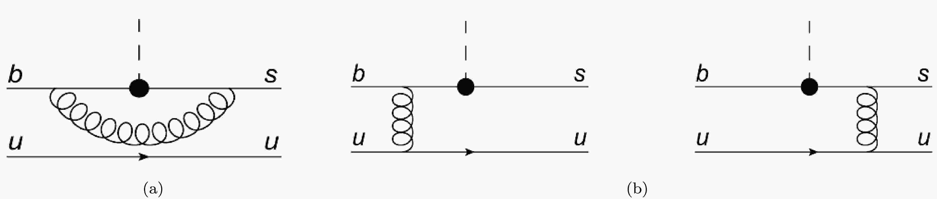
$ {\cal{O}}(\alpha_s) $ , these symmetry relations acquire corrections from vertex and hard-spectator interactions, as illustrated in Fig. (1). In this section, we evaluate these two types of corrections separately.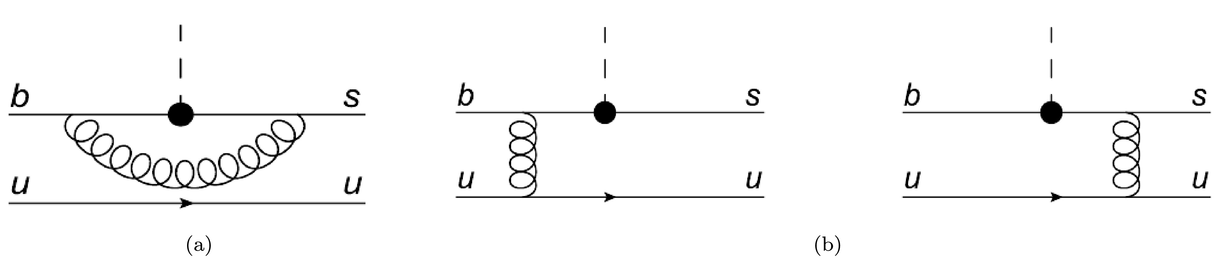
Figure 1. Vertex and Hard-Spectator Corrections in B to
$ K^{*}_0(1430) $ Decays.Since the hard and soft contributions associated with Fig. (1-b) cannot be uniquely separated and exhibit logarithmic divergences, a suitable factorization framework is required. For a detailed discussion of this approach, see Beneke et al. [42] and Refs. [36, 65, 66]. The factorization formula for heavy-to-light transitions at large recoil, valid at leading order in
$ 1/m_b $ , can be summarized as follows:$ f_i(q^2)=C_i\xi_{K^{*}_0}(E_F)+\Phi_B\otimes {\cal{T}}^\Gamma\otimes \Phi_{K^{*}_0}, $
(23) where
$ \xi_{K^{*}_0}(E_F) $ is the soft form factor to which the symmetry relations derived above apply. The quantity$ {\cal{T}}^\Gamma $ represents a hard-scattering kernel that is convolved with the light-cone distribution amplitudes$ \Phi_B $ and$ \Phi_{K^{*}_0} $ of the B and$ K^{*}_0 $ mesons, respectively. The coefficients$ C_i=1+{\cal{O}}(\alpha_s) $ account for vertex and hard-spectator renormalization effects, which we compute below using the vertex and hard-spectator interaction diagrams. -
In the previous section, we showed that HQS relates the various form factors [cf. Eq. (22)]. However, at
$ {\cal{O}}(\alpha_s) $ , these symmetry relations acquire corrections from vertex and hard-spectator interactions, as illustrated in Fig. 1. In this section, we evaluate these two types of corrections separately.
Figure 1. Vertex and Hard-Spectator Corrections in B to
$ K^{*}_0(1430) $ Decays.Since the hard and soft contributions associated with Fig. 1(b) cannot be uniquely separated and exhibit logarithmic divergences, a suitable factorization framework is required. For a detailed discussion of this approach, see Beneke et al. [42] and Refs. [36, 65, 66]. The factorization formula for heavy-to-light transitions at large recoil, valid at leading order in
$ 1/m_b $ , can be summarized as follows:$ f_i(q^2)=C_i\xi_{K^{*}_0}(E_F)+\Phi_B\otimes {\cal{T}}^\Gamma\otimes \Phi_{K^{*}_0}, $
(23) where
$ \xi_{K^{*}_0}(E_F) $ is the soft form factor to which the symmetry relations derived above apply. The quantity$ {\cal{T}}^\Gamma $ represents a hard-scattering kernel that is convolved with the light-cone distribution amplitudes$ \Phi_B $ and$ \Phi_{K^{*}_0} $ of the B and$ K^{*}_0 $ mesons, respectively. The coefficients$ C_i=1+ {\cal{O}}(\alpha_s) $ account for vertex and hard-spectator renormalization effects, which we compute below using the vertex and hard-spectator interaction diagrams. -
The one-loop diagram, Fig. (1-a), contains both ultraviolet (UV) and infrared (IR) divergences. The UV divergences are treated using dimensional regularization
$ (d=4-2\epsilon) $ , whereas the infrared divergences are handled by introducing a small parameter λ, i.e., a gluon mass term. Employing the standard Passarino-Veltman reduction techniques and retaining the finite mass term$ m^2_{K^{*}_0} $ , the one-loop results for the Dirac structure Γ are given by [41, 42]:$ \begin{aligned}[b]& \bar{u}(p')\Gamma(p',p)u(p)\\=\;&\frac{\alpha_sC_F}{4\pi}\bar{u}(p')\Bigg[\Bigg\{-\frac{1}{2}{\rm{ln}}\left(\frac{\lambda^2m_{b}^{2}}{m_{b}^{2}-q^2}\right)-2{\rm{ln}}\left(\frac{\lambda^2m_{b}^{2}}{(m_{b}^{2}-q^2)^2}\right) \\ &-2{\rm{Li}}_2\left(\frac{q^2}{m_{b}^2}\right)+\frac{2m^2_B}{m^2_B-q^2}L-3-\frac{\pi^2}{2}\Bigg\}\Gamma \\&+\frac{1}{4}\left\lbrace\frac{1}{\hat{\epsilon}}+3-{\rm{ln}}\left(\frac{m_b ^2}{\mu^2}\right)-L'\right\rbrace \gamma^\alpha\gamma^\beta\Gamma\gamma_{\beta}\gamma_{\alpha} \\ &+\frac{1}{2q^2}\left\lbrace 1-\frac{ m_B}{2 E_F}L\right\rbrace \gamma^{\alpha}\not{p}\Gamma\not{p^{'}}\gamma_{\alpha}+\frac{1}{2q^2}\left\lbrace 1-L^{\prime}\right\rbrace m_b \gamma^{\alpha}\not{p}\Gamma \gamma_{\alpha} \\ &-\left.\frac{1}{2q^2}\left\lbrace 2-L^{\prime\prime }\right\rbrace m_b \Gamma \not{p'}\right] u(p)\;, \end{aligned} $
(24) Here,
$ \bar{u}(p') $ and$ u(p) $ denote the external Dirac spinors for the light and heavy quarks, respectively. The above expression is derived using the on-shell relations$ \bar{u}(p')\not{p'}=0 $ and$ \not{p}u(p)=m_bu(p) $ . The pole$ \dfrac{1}{\hat{\epsilon}} $ is defined as$ \dfrac{1}{\epsilon} -\gamma_E +\ln 4 \pi $ and is subtracted in the$ \overline{{\rm{MS}}} $ scheme. Here, the momentum transfer is$ q^2=m_B^2+m_{K^{*}_0} ^2-2m_B E_F $ , as mentioned earlier. For convenience, we introduce abbreviations for the remaining terms as follows:$ \begin{aligned} L&=-\frac{2E_F}{m_B-2E_F +\frac{m_{K^{*}_0} ^2}{m_B}}\ln\left(\frac{2E_F}{ m_B}-\frac{m_{K^{*}_0} ^2}{ m_B^2}\right),\nonumber\\ L^{\prime}&=L\left(1-\frac{m_{K^{*}_0} ^2}{2E_F m_B}\right),\nonumber\\ L^{\prime\prime}&=L\left(4-\frac{m_B }{E_F}-\frac{2m_{K^{*}_0} ^2}{E_F m_B}\right)\;. \nonumber \label{vertex} \end{aligned} $
It is convenient to fix the renormalization convention for soft form factors by imposing the following condition, which holds to all orders in perturbation theory [41].
$ f_+(q^2)=\left(1+\frac{m^2_{K^{*}_0}}{m_B^2}\right)\xi_{K^{*}_0}(E_F) $
(25) Once the factorization scheme is specified, the
$ {\cal{O}}(\alpha_s) $ contributions for any given Dirac current Γ can be calculated by inserting Γ into Eq.(14). Applying the renormalization convention in Eq.(25) and then comparing the result with the form-factor expressions in Eq.(17), we obtain the following results.$ \begin{aligned}[b] f_-(q^2) =\;& -\xi_{K_0^{*}}\Bigg[ \frac{\left(1 + \dfrac{m_{K_0^{*}}^2}{m_B^2}\right)}{\left(1 - \dfrac{2m_{K_0^{*}}^2}{m_B^2}\right)} - \frac{\alpha_s C_F E_F}{4\pi} \Bigg\{ \frac{m_{K_0^{*}}^4+4 \Delta E m_{K_0^{*}}^2}{2 E^2 \Delta} \left( \dfrac{1-\dfrac{m_B}{2 E_f} L}{2 q^2} -\dfrac{2-L^{\prime\prime}}{2 q^2} \right) \\ & - \frac{m_{K_0^{*}}^2}{m_B E\,\Delta} \left( \frac{2m_B^2}{m_B^2 - q^2}L- L^\prime - \ln \frac{m_b^2}{\mu^2} + 3 \right) + 4m_B \left(\frac{1 - L^\prime}{q^2}\right) - \frac{m_{K_0^{*}}^4}{ E^2\Delta} \left( \frac{1 - \dfrac{m_B }{2E_F}L}{2 q^2} \right) \Bigg\} \Bigg]\;, \end{aligned} $
(26) and the expression for
$ f_T $ is given as$ \begin{aligned}[b] f_T(q^2)=\;&\xi_{K_0^{*}}\Bigg[ \left(\frac{m_B+m_{K_0^{*}}}{m_B}\right) \left(\frac{m_B^2+m_{K_0^{*}}^2}{m_B^2-m_{K_0^{*}}^2}\right) +\frac{\alpha_s C_F E_F}{4\pi} \frac{ m_B(m_B+m_{K_0^{*}}) }{(E_F m_B - m_{K_0^{*}}^2)}\times \Bigg\{ \left( \frac{1}{m_B}+\frac{m_{K_0^{*}}^2}{2E\Delta m_B} -\frac{m_{K_0^{*}}^2}{E m_B^2} -\frac{m_{K_0^{*}}^4}{4E^2\Delta m_B^2} \right)\frac{2m_B^2}{m_B^2-q^2}L \\ &+\left( -4\Delta-\frac{2m_{K_0^{*}}^2}{E} +\frac{4m_{K_0^{*}}^2}{m_B} \right)\frac{1-\dfrac{m_B}{2E_F}L}{2q^2} +\left( 4m_B+\frac{m_B m_{K_0^{*}}^2}{E\Delta} -\frac{3m_{K_0^{*}}^2}{E} -\frac{m_{K_0^{*}}^4}{2E^2\Delta} \right)\frac{1-L^\prime}{2q^2} \\ &+\left( -2\Delta+\frac{m_{K_0^{*}}^4}{2E\Delta m_B} -\frac{m_{K_0^{*}}^4}{4E^2\Delta} +\frac{m_{K_0^{*}}^2}{m_B} -\frac{m_{K_0^{*}}^2}{E} \right)\frac{2-L^{\prime\prime}}{2q^2} \Bigg\}\Bigg] \end{aligned} $
(27) -
The one-loop diagram, Fig. 1(a), contains both ultraviolet (UV) and infrared (IR) divergences. The UV divergences are treated using dimensional regularization
$ (d=4-2\epsilon) $ , whereas the infrared divergences are handled by introducing a small parameter λ, i.e., a gluon mass term. Employing the standard Passarino-Veltman reduction techniques and retaining the finite mass term$ m^2_{K^{*}_0} $ , the one-loop results for the Dirac structure Γ are given by [41, 42]:$ \begin{aligned}[b]& \bar{u}(p')\Gamma(p',p)u(p)\\=\;&\frac{\alpha_sC_F}{4\pi}\bar{u}(p')\Bigg[\Bigg\{-\frac{1}{2}{\rm{ln}}\left(\frac{\lambda^2m_{b}^{2}}{m_{b}^{2}-q^2}\right)-2{\rm{ln}}\left(\frac{\lambda^2m_{b}^{2}}{(m_{b}^{2}-q^2)^2}\right) \\ &-2{\rm{Li}}_2\left(\frac{q^2}{m_{b}^2}\right)+\frac{2m^2_B}{m^2_B-q^2}L-3-\frac{\pi^2}{2}\Bigg\}\Gamma \\&+\frac{1}{4}\left\lbrace\frac{1}{\hat{\epsilon}}+3-{\rm{ln}}\left(\frac{m_b ^2}{\mu^2}\right)-L'\right\rbrace \gamma^\alpha\gamma^\beta\Gamma\gamma_{\beta}\gamma_{\alpha} \\ &+\frac{1}{2q^2}\left\lbrace 1-\frac{ m_B}{2 E_F}L\right\rbrace \gamma^{\alpha}\not{p}\Gamma\not{p}' \gamma_{\alpha}+\frac{1}{2q^2}\left\lbrace 1-L^{\prime}\right\rbrace m_b \gamma^{\alpha}\not{p}\Gamma \gamma_{\alpha} \\ &-\left.\frac{1}{2q^2}\left\lbrace 2-L^{\prime\prime }\right\rbrace m_b \Gamma \not{p'}\right] u(p)\;. \end{aligned} $
(24) Here,
$ \bar{u}(p') $ and$ u(p) $ denote the external Dirac spinors for the light and heavy quarks, respectively. The above expression is derived using the on-shell relations$ \bar{u}(p')\not{p'}=0 $ and$ \not{p}u(p)=m_bu(p) $ . The pole$ \dfrac{1}{\hat{\epsilon}} $ is defined as$ \dfrac{1}{\epsilon} -\gamma_E + \ln 4 \pi $ and is subtracted in the$ \overline{{\rm{MS}}} $ scheme. Here, the momentum transfer is$ q^2=m_B^2+m_{K^{*}_0} ^2-2m_B E_F $ , as mentioned earlier. For convenience, we introduce abbreviations for the remaining terms as follows:$ \begin{aligned} L&=-\frac{2E_F}{m_B-2E_F +\dfrac{m_{K^{*}_0} ^2}{m_B}}\ln\left(\frac{2E_F}{ m_B}-\frac{m_{K^{*}_0} ^2}{ m_B^2}\right),\nonumber\\ L^{\prime}&=L\left(1-\frac{m_{K^{*}_0} ^2}{2E_F m_B}\right),\nonumber\\ L^{\prime\prime}&=L\left(4-\frac{m_B }{E_F}-\frac{2m_{K^{*}_0} ^2}{E_F m_B}\right)\;. \nonumber \label{vertex} \end{aligned} $
It is convenient to fix the renormalization convention for soft form factors by imposing the following condition, which holds to all orders in perturbation theory [41]
$ f_+(q^2)=\left(1+\frac{m^2_{K^{*}_0}}{m_B^2}\right)\xi_{K^{*}_0}(E_F). $
(25) Once the factorization scheme is specified, the
$ {\cal{O}}(\alpha_s) $ contributions for any given Dirac current Γ can be calculated by inserting Γ into Eq. (14). Applying the renormalization convention in Eq. (25) and then comparing the result with the form-factor expressions in Eq. (17), we obtain the following results$ \begin{aligned}[b] f_-(q^2) =\;& -\xi_{K_0^{*}} \left[ \frac{\left(1 + \dfrac{m_{K_0^{*}}^2}{m_B^2}\right)}{\left(1 - \dfrac{2m_{K_0^{*}}^2}{m_B^2}\right)} - \frac{\alpha_s C_F E_F}{4\pi} \left\{ \frac{m_{K_0^{*}}^4+4 \Delta E m_{K_0^{*}}^2}{2 E^2 \Delta} \left( \dfrac{1-\dfrac{m_B}{2 E_f} L}{2 q^2} -\dfrac{2-L^{\prime\prime}}{2 q^2} \right) \right.\right. \\ & \left. \left. - \frac{m_{K_0^{*}}^2}{m_B E\,\Delta} \left( \frac{2m_B^2}{m_B^2 - q^2}L- L^\prime - \ln \frac{m_b^2}{\mu^2} + 3 \right) + 4m_B \left(\frac{1 - L^\prime}{q^2}\right) - \frac{m_{K_0^{*}}^4}{ E^2\Delta} \left( \frac{1 - \dfrac{m_B }{2E_F}L}{2 q^2} \right) \right\} \right]\;, \end{aligned} $
(26) and the expression for
$ f_T $ is given as$ \begin{aligned}[b] f_T(q^2)=\;&\xi_{K_0^{*}}\Bigg[ \left(\frac{m_B+m_{K_0^{*}}}{m_B}\right) \left(\frac{m_B^2+m_{K_0^{*}}^2}{m_B^2-m_{K_0^{*}}^2}\right) +\frac{\alpha_s C_F E_F}{4\pi} \frac{ m_B(m_B+m_{K_0^{*}}) }{(E_F m_B - m_{K_0^{*}}^2)} \Bigg\{ \left( \frac{1}{m_B}+\frac{m_{K_0^{*}}^2}{2E\Delta m_B} -\frac{m_{K_0^{*}}^2}{E m_B^2} -\frac{m_{K_0^{*}}^4}{4E^2\Delta m_B^2} \right)\frac{2m_B^2}{m_B^2-q^2}L \\ &+\left( -4\Delta-\frac{2m_{K_0^{*}}^2}{E} +\frac{4m_{K_0^{*}}^2}{m_B} \right)\frac{1-\dfrac{m_B}{2E_F}L}{2q^2} +\left( 4m_B+\frac{m_B m_{K_0^{*}}^2}{E\Delta} -\frac{3m_{K_0^{*}}^2}{E} -\frac{m_{K_0^{*}}^4}{2E^2\Delta} \right)\frac{1-L^\prime}{2q^2} \\ &+\left( -2\Delta+\frac{m_{K_0^{*}}^4}{2E\Delta m_B} -\frac{m_{K_0^{*}}^4}{4E^2\Delta} +\frac{m_{K_0^{*}}^2}{m_B} -\frac{m_{K_0^{*}}^2}{E} \right)\frac{2-L^{\prime\prime}}{2q^2} \Bigg\}\Bigg]. \end{aligned} $
(27) -
The form factors calculated above receive additional corrections from interactions with spectator quarks, denoted by
$ \Delta f_{-,T} $ . These hard-spectator corrections arise at$ {\cal{O}}\left(\alpha_s\right) $ when the active quark interacts with the spectator quark, as shown in Fig. 1-b. The momenta of the heavy b quark and the spectator quark in the B meson are defined as:$ p^\mu=m_bv^\mu, \quad l^\mu=\frac{l_+}{2}n^\mu_++l^\mu_\perp+\frac{l_-}{2}n^\mu_- $
(28) The momenta of the s quark and the spectator quark in the final-state
$ K_0^{*} $ meson are given by$\begin{aligned}[b]& k^\mu_1=uE_Fn^\mu_-+k^\mu_\perp+\left(\frac{\vec{k}^2_\perp}{4uE_F}+\frac{m^2_{K^{*}_0}}{4uE_F}\right)n^\mu_+\;, \\& k^\mu_2=\bar{u}E_Fn^\mu_--k^\mu_\perp+\left(\frac{\vec{k}^2_\perp}{4\bar{u}E_F}+\frac{m^2_{K^{*}_0}}{4uE_F}\right)n^\mu_+\;,\end{aligned} $
(29) where
$ \bar{u}=1-u $ . All components of the spectator momenta, l,$ k_1 $ , and$ k_2 $ , are of order$ \Lambda_{\rm{QCD}} $ . The final-state meson momentum satisfies$ (k_1+k_2)^2\sim m_{K_0^{*}}^2 $ , which would otherwise scale as$ \Lambda_{\rm{QCD}}^2 $ and could be neglected at leading order. Consequently, the exchange of a hard gluon with momentum of order$ m_B\Lambda_{\rm{QCD}} $ becomes relevant along the$ n_- $ direction.The hard-spectator contribution to the heavy-to-light current matrix element can therefore be expressed in terms of the convolution formula
$ \langle K^{*}_0|\bar{q}\Gamma b|B\rangle=\frac{4\pi\alpha_s C_F}{N_C}\int^1_0 du\int^\infty_0 dl_+ {\cal{M}}^B_{jk} {\cal{M}}^{k^{*}_0}_{li} {\cal{T}}^\Gamma _{ijkl}\;. $
(30) Here,
$ \Gamma=\gamma^\mu\gamma_5 $ or$ \sigma^\mu{}^\nu \gamma_5q_\nu $ , and$ {\cal{T}}^\Gamma _{ijkl} $ denotes the hard-scattering amplitude computed from the Feynman diagrams shown in Fig. 1-b. The quantities$ {\cal{M}}^B $ and$ {\cal{M}}^{K^{*}_0} $ are the two light-cone projectors that encode the nonperturbative dynamics of the initial and final-state bound mesons. The$ K^{*}_0 $ -meson projector is given in Refs. [41, 75]$ {\cal{M}}^{K_0^{*}}_{li} = \frac{\bar f_{K_0^{*}}}{4} \Bigg[ \not{p_F}\, \phi_{K_0^{*}}(u) + m_{K_0^{*}}\, \phi_{K_0^{*}}^s(u) + m_{K_0^{*}}\, \sigma_{\mu\nu}\, p_F^\mu n^\nu\, \frac{\phi_{K_0^{*}}^\sigma(u)}{6} \Bigg]_{li}\;, $
(31) where
$ f_{K^{*}_0} $ is the$ K_0^{*} $ decay constant,$ \phi_{K_0^{*}}(u) $ is the twist-2 light-cone distribution amplitude, and$ \phi_{K_0^{*}}^s(u) $ and$ \phi_{K_0^{*}}^\sigma(u) $ are the twist-3 light-cone distribution amplitudes for the scalar meson$ {K_0^{*}} $ . Further details can be found in Appendix A. Correspondingly, the heavy-meson projector used in this calculation is:$\begin{aligned}[b] {\cal{M}}^{B}_{jk} =\;& -\frac{i f_B m_B}{4} \Bigg[ \frac{1+\not{v}}{2} \Bigg\{ \phi_+^B(l_+)\,\not{n}_+ \\&+ \phi_-^B(l_+) \left( \not{n}_- - l_+\,\gamma^\nu_\perp \frac{\partial}{\partial l^\nu_\perp} \right) \Bigg\} \gamma_5 \Bigg]_{jk} \Bigg|_{\,l=\frac{l_+}{2}n_+}\;, \end{aligned}$
(32) where
$ \phi_+^B(l_+) $ and$ \phi_-^B(l_+) $ denote the distribution amplitudes of the B meson, as discussed in Appendix B. The hard-scattering amplitude in Feynman gauge takes the following form:$\begin{aligned}[b] {\cal{T}}_{ijkl}^\Gamma=\;&\Bigg[\Gamma\frac{m_b(1+\not{v})+\not{l}-\not{k_2}}{(m_bv+l-k_2)^2-m^2_b}\gamma_\mu+\gamma_\mu\frac{\not{k}_1+\not{k}_2-\not{l}}{(k_1+k_2-l)^2}\Gamma\Bigg]_{i{}_j}\\&\times\frac{1}{(l-k_2)^2}[\gamma^\mu]_{k{}_l}\;. \end{aligned}$
(33) The gluon momenta give
$ (l-k_2)^2 \sim -2\,l_+\,\bar{u}\,E_F $ , and the numerator of the first term gives$ \not{l}-\not{k}_2 \sim -\bar{u}E_F\not{n}_- $ ; both of these terms are of order$ m_B\Lambda_{\rm{QCD}} $ , and they contribute together with the leading term$ m_b(1+\not{v}) $ . The total contribution from hard-gluon exchange, neglecting terms of order$ \Lambda_{\rm{QCD}}/m_B $ in the hard-spectator kernel, is given by$ {\cal{T}}_{ijkl}^\Gamma\simeq\left[\Gamma\frac{m_b(1+\not{v})-\bar{u}E_F\not{n}_-}{4\bar{u}^2l_+m_bE^2_F}\gamma^\mu+\gamma^\mu\frac{E_F\not{n}_- -\not{l}}{4\bar{u}l^2_+E^2_F}\Gamma\right]_{i{}_j}[\gamma^\mu]_{k{}_l}\;. $
(34) The term
$ m_b(1+\not{v}) $ exhibits a logarithmic divergence in the limit$ \bar{u}\to 0 $ because the distribution amplitude (DA)$ \phi(u) $ vanishes linearly at leading twist. These endpoint divergences do not violate the symmetry relations and can be absorbed into the soft form factors within the factorization scheme of Eq. (23). This can be verified from the current structure defined in Eq. (14).In this analysis, we employ the twist-2 distribution amplitude, which provides the leading-twist contribution, whereas the twist-3 distribution amplitudes are suppressed by a factor of
$ 1/m_B $ . However, this suppression is compensated by an enhancement in$ {\cal{M}}^{K_0^{*}} $ in the endpoint limit$ \bar{u}\to 0 $ . Consequently, these terms contribute at leading order to the soft form factors$ \xi_{K_0^{*}} $ . The details of the leading-order terms in the hard-scattering kernel, together with the underlying power-counting framework, can be found in [41].The contributions from hard-spectator interactions are presented in detail for the case of
$ f_-(q^2) $ . Similar calculations can be performed for$ f_T\left(q^2\right) $ as well. These contributions are denoted by$ \Delta F_P $ and are expressed as$ \Delta F_P=\frac{8\pi^2f_Bf_{K_0^{*}}}{N_cm_B}\langle l_+^{-1}\rangle_+\langle\bar{u}^{-1}\rangle_P\;. $
(35) Evaluation of these corrections requires the moments of the distribution amplitudes
$ \langle l_+^{-1}\rangle_+ $ and$ \langle\bar{u}^{-1}\rangle $ for the B-meson and the scalar meson$ K^{*}_0 $ , respectively, given by$ \langle l_+^{-1}\rangle_+ =\int dl_+\frac{\phi^B_+(l_+)}{l_+}\;, $
(36) $ \langle\bar{u}^{-1}\rangle =\int du\frac{\phi^{K_0^{*}}(u)}{\bar{u}}\;. $
(37) With the help of these expressions, we can calculate the hard-spectator corrections to the
$ B\to K^{*}_0 $ form factors$ \Delta f_i $ . However, the renormalization condition in Eq.(25) implies$ \Delta f_+=0 $ by definition. The remaining two form factors are then given by$ \Delta f_-=\frac{m_B^2-m_{K_0^{*}}^2}{2E_F m_B}\Delta F_P\;, \quad \Delta f_T=-\frac{m_B+m_{K_0^{*}}}{2E_F}\Delta F_P \;. $
The total
$ {\cal{O}}(\alpha_s) $ correction is given by the sum of the vertex and hard-spectator corrections. Combining these corrections yields:$ \begin{aligned}[b] f_-(q^2) =\;& -\xi_{K_0^{*}}\Bigg[ \frac{\left(1 + \dfrac{m_{K_0^{*}}^2}{m_B^2}\right)}{\left(1 - \dfrac{2m_{K_0^{*}}^2}{m_B^2}\right)} - \frac{\alpha_s C_F E_F}{4\pi} \Bigg\{ \frac{m_{K_0^{*}}^4+4 \Delta E m_{K_0^{*}}^2}{2 E^2 \Delta} \left( \dfrac{1-\dfrac{m_B}{2 E_f} L}{2 q^2} -\dfrac{2-L^{\prime\prime}}{2 q^2} \right) \\ & - \frac{m_{K_0^{*}}^2}{m_B E\,\Delta} \left( \frac{2m_B^2}{m_B^2 - q^2}L- L^\prime - \ln \frac{m_b^2}{\mu^2} + 3 \right) + 4m_B \left(\frac{1 - L^\prime}{q^2}\right) - \frac{m_{K_0^{*}}^4}{ E^2\Delta} \left( \frac{1 - \dfrac{m_B }{2E_F}L}{2 q^2} \right) \Bigg\} \Bigg] + \frac{\alpha_s C_F}{4\pi} \left( \frac{m_B^2-m_{K_0^{*}}^2}{2E_F m_B} \right) \Delta F_P \;, \end{aligned} $
(38) and
$ \begin{aligned}[b] f_T(q^2)=\;&\xi_{K_0^{*}}\Bigg[ \left(\frac{m_B+m_{K_0^{*}}}{m_B}\right) \left(\frac{m_B^2+m_{K_0^{*}}^2}{m_B^2-m_{K_0^{*}}^2}\right) +\frac{\alpha_s C_F E_F}{4\pi} \frac{ m_B(m_B+m_{K_0^{*}}) }{(E_F m_B - m_{K_0^{*}}^2)} \Bigg\{ \left( \frac{1}{m_B}+\frac{m_{K_0^{*}}^2}{2E\Delta m_B} -\frac{m_{K_0^{*}}^2}{E m_B^2} -\frac{m_{K_0^{*}}^4}{4E^2\Delta m_B^2} \right)\frac{2m_B^2}{m_B^2-q^2}L \\ &+\left( -4\Delta-\frac{2m_{K_0^{*}}^2}{E} +\frac{4m_{K_0^{*}}^2}{m_B} \right)\frac{1-\dfrac{m_B}{2E_F}L}{2q^2} +\left( 4m_B+\frac{m_B m_{K_0^{*}}^2}{E\Delta} -\frac{3m_{K_0^{*}}^2}{E} -\frac{m_{K_0^{*}}^4}{2E^2\Delta} \right)\frac{1-L^\prime}{2q^2} \\ &+\left( -2\Delta+\frac{m_{K_0^{*}}^4}{2E\Delta m_B} -\frac{m_{K_0^{*}}^4}{4E^2\Delta} +\frac{m_{K_0^{*}}^2}{m_B} -\frac{m_{K_0^{*}}^2}{E} \right)\frac{2-L^{\prime\prime}}{2q^2} \Bigg\}\Bigg]-\frac{\alpha_s C_F}{4\pi}\left(\frac{m_B+m_{K_0^{*}}}{2E_F}\right)\Delta F_P\;. \end{aligned} $
(39) -
The form factors calculated above receive additional corrections from interactions with spectator quarks, denoted by
$ \Delta f_{-,T} $ . These hard-spectator corrections arise at$ {\cal{O}}\left(\alpha_s\right) $ when the active quark interacts with the spectator quark, as shown in Fig. 1(b). The momenta of the heavy b quark and the spectator quark in the B meson are defined as:$ p^\mu=m_bv^\mu, \quad l^\mu=\frac{l_+}{2}n^\mu_++l^\mu_\perp+\frac{l_-}{2}n^\mu_- \; .$
(28) The momenta of the s quark and the spectator quark in the final-state
$ K_0^{*} $ meson are given by$\begin{aligned}[b]& k^\mu_1=uE_Fn^\mu_-+k^\mu_\perp+\left(\frac{\vec{k}^2_\perp}{4uE_F}+\frac{m^2_{K^{*}_0}}{4uE_F}\right)n^\mu_+\;, \\& k^\mu_2=\bar{u}E_Fn^\mu_--k^\mu_\perp+\left(\frac{\vec{k}^2_\perp}{4\bar{u}E_F}+\frac{m^2_{K^{*}_0}}{4uE_F}\right)n^\mu_+\;,\end{aligned} $
(29) where
$ \bar{u}=1-u $ . All components of the spectator momenta, l,$ k_1 $ , and$ k_2 $ , are of order$ \Lambda_{\rm{QCD}} $ . The final-state meson momentum satisfies$ (k_1+k_2)^2\sim m_{K_0^{*}}^2 $ , which would otherwise scale as$ \Lambda_{\rm{QCD}}^2 $ and could be neglected at leading order. Consequently, the exchange of a hard gluon with momentum of order$ m_B\Lambda_{\rm{QCD}} $ becomes relevant along the$ n_- $ direction.The hard-spectator contribution to the heavy-to-light current matrix element can therefore be expressed in terms of the convolution formula
$ \langle K^{*}_0|\bar{q}\Gamma b|B\rangle=\frac{4\pi\alpha_s C_F}{N_C}\int^1_0 {\rm d} u\int^\infty_0 {\rm d} l_+ {\cal{M}}^B_{jk} {\cal{M}}^{k^{*}_0}_{li} {\cal{T}}^\Gamma _{ijkl}\;. $
(30) Here,
$ \Gamma=\gamma^\mu\gamma_5 $ or$ \sigma^\mu{}^\nu \gamma_5q_\nu $ , and$ {\cal{T}}^\Gamma _{ijkl} $ denotes the hard-scattering amplitude computed from the Feynman diagrams shown in Fig. 1(b). The quantities$ {\cal{M}}^B $ and$ {\cal{M}}^{K^{*}_0} $ are the two light-cone projectors that encode the nonperturbative dynamics of the initial and final-state bound mesons. The$ K^{*}_0 $ -meson projector is given in Refs. [41, 67]$ {\cal{M}}^{K_0^{*}}_{li} = \frac{\bar f_{K_0^{*}}}{4} \Bigg[ \not{p_F}\, \phi_{K_0^{*}}(u) + m_{K_0^{*}}\, \phi_{K_0^{*}}^s(u) + m_{K_0^{*}}\, \sigma_{\mu\nu}\, p_F^\mu n^\nu\, \frac{\phi_{K_0^{*}}^\sigma(u)}{6} \Bigg]_{li}\;, $
(31) where
$ f_{K^{*}_0} $ is the$ K_0^{*} $ decay constant,$ \phi_{K_0^{*}}(u) $ is the twist-2 light-cone distribution amplitude, and$ \phi_{K_0^{*}}^s(u) $ and$ \phi_{K_0^{*}}^\sigma(u) $ are the twist-3 light-cone distribution amplitudes for the scalar meson$ {K_0^{*}} $ . Further details can be found in Appendix A. Correspondingly, the heavy-meson projector used in this calculation is:$\begin{aligned}[b] {\cal{M}}^{B}_{jk} =\;& -\frac{{\rm i} f_B m_B}{4} \Bigg[ \frac{1+\not{\,v}}{2} \Bigg\{ \phi_+^B(l_+)\,\not{n}_+ \\&+ \phi_-^B(l_+) \left( \not{\,n}_- - l_+\,\gamma^\nu_\perp \frac{\partial}{\partial l^\nu_\perp} \right) \Bigg\} \gamma_5 \Bigg]_{jk} \Bigg|_{\,l=\frac{l_+}{2}n_+}\;, \end{aligned}$
(32) where
$ \phi_+^B(l_+) $ and$ \phi_-^B(l_+) $ denote the distribution amplitudes of the B meson, as discussed in Appendix B. The hard-scattering amplitude in Feynman gauge takes the following form:$\begin{aligned}[b] {\cal{T}}_{ijkl}^\Gamma=\;&\Bigg[\Gamma\frac{m_b(1+\not{\,v})+\not{\,l}-\not{k_2}}{(m_bv+l-k_2)^2-m^2_b}\gamma_\mu+\gamma_\mu\frac{\not{k}_1+\not{k}_2-\not{\,l}}{(k_1+k_2-l)^2}\Gamma\Bigg]_{i{}_j}\\&\times\frac{1}{(l-k_2)^2}[\gamma^\mu]_{k{}_l}\;. \end{aligned}$
(33) The gluon momenta give
$ (l-k_2)^2 \sim -2\,l_+\,\bar{u}\,E_F $ , and the numerator of the first term gives$ \not{\,l}-\not{k}_2 \sim -\bar{u}E_F\not{\,n}_- $ ; both of these terms are of order$ m_B\Lambda_{\rm{QCD}} $ , and they contribute together with the leading term$ m_b(1+\not{\,v}) $ . The total contribution from hard-gluon exchange, neglecting terms of order$ \Lambda_{\rm{QCD}}/m_B $ in the hard-spectator kernel, is given by$ {\cal{T}}_{ijkl}^\Gamma\simeq\left[\Gamma\frac{m_b(1+\not{\,v})-\bar{u}E_F\not{\,n}_-}{4\bar{u}^2l_+m_bE^2_F}\gamma^\mu+\gamma^\mu\frac{E_F\not{\,n}_- -\not{\,l}}{4\bar{u}l^2_+E^2_F}\Gamma\right]_{i{}_j}[\gamma^\mu]_{k{}_l}\;. $
(34) The term
$ m_b(1+\not{\,v}) $ exhibits a logarithmic divergence in the limit$ \bar{u}\to 0 $ because the distribution amplitude (DA)$ \phi(u) $ vanishes linearly at leading twist. These endpoint divergences do not violate the symmetry relations and can be absorbed into the soft form factors within the factorization scheme of Eq. (23). This can be verified from the current structure defined in Eq. (14).In this analysis, we employ the twist-2 distribution amplitude, which provides the leading-twist contribution, whereas the twist-3 distribution amplitudes are suppressed by a factor of
$ 1/m_B $ . However, this suppression is compensated by an enhancement in$ {\cal{M}}^{K_0^{*}} $ in the endpoint limit$ \bar{u}\to 0 $ . Consequently, these terms contribute at leading order to the soft form factors$ \xi_{K_0^{*}} $ . The details of the leading-order terms in the hard-scattering kernel, together with the underlying power-counting framework, can be found in [41].The contributions from hard-spectator interactions are presented in detail for the case of
$ f_-(q^2) $ . Similar calculations can be performed for$ f_T\left(q^2\right) $ as well. These contributions are denoted by$ \Delta F_P $ and are expressed as$ \Delta F_P=\frac{8\pi^2f_Bf_{K_0^{*}}}{N_cm_B}\langle l_+^{-1}\rangle_+\langle\bar{u}^{-1}\rangle_P\;. $
(35) Evaluation of these corrections requires the moments of the distribution amplitudes
$ \langle l_+^{-1}\rangle_+ $ and$ \langle\bar{u}^{-1}\rangle $ for the B-meson and the scalar meson$ K^{*}_0 $ , respectively, given by$ \langle l_+^{-1}\rangle_+ =\int {\rm d} l_+\frac{\phi^B_+(l_+)}{l_+}\;, $
(36) $ \langle\bar{u}^{-1}\rangle =\int {\rm d} u\frac{\phi^{K_0^{*}}(u)}{\bar{u}}\;. $
(37) With the help of these expressions, we can calculate the hard-spectator corrections to the
$ B\to K^{*}_0 $ form factors$ \Delta f_i $ . However, the renormalization condition in Eq. (25) implies$ \Delta f_+=0 $ by definition. The remaining two form factors are then given by$ \Delta f_-=\frac{m_B^2-m_{K_0^{*}}^2}{2E_F m_B}\Delta F_P\;, \quad \Delta f_T=-\frac{m_B+m_{K_0^{*}}}{2E_F}\Delta F_P \;. $
The total
$ {\cal{O}}(\alpha_s) $ correction is given by the sum of the vertex and hard-spectator corrections. Combining these corrections yields:$ \begin{aligned}[b] f_-(q^2) =\;& -\xi_{K_0^{*}}\Bigg[ \frac{\left(1 + \dfrac{m_{K_0^{*}}^2}{m_B^2}\right)}{\left(1 - \dfrac{2m_{K_0^{*}}^2}{m_B^2}\right)} - \frac{\alpha_s C_F E_F}{4\pi} \Bigg\{ \frac{m_{K_0^{*}}^4+4 \Delta E m_{K_0^{*}}^2}{2 E^2 \Delta} \left( \dfrac{1-\dfrac{m_B}{2 E_f} L}{2 q^2} -\dfrac{2-L^{\prime\prime}}{2 q^2} \right) \\ & - \frac{m_{K_0^{*}}^2}{m_B E\,\Delta} \left( \frac{2m_B^2}{m_B^2 - q^2}L- L^\prime - \ln \frac{m_b^2}{\mu^2} + 3 \right) + 4m_B \left(\frac{1 - L^\prime}{q^2}\right) - \frac{m_{K_0^{*}}^4}{ E^2\Delta} \left( \frac{1 - \dfrac{m_B }{2E_F}L}{2 q^2} \right) \Bigg\} \Bigg] + \frac{\alpha_s C_F}{4\pi} \left( \frac{m_B^2-m_{K_0^{*}}^2}{2E_F m_B} \right) \Delta F_P \;, \end{aligned} $
(38) and
$ \begin{aligned}[b] f_T(q^2)=\;&\xi_{K_0^{*}}\Bigg[ \left(\frac{m_B+m_{K_0^{*}}}{m_B}\right) \left(\frac{m_B^2+m_{K_0^{*}}^2}{m_B^2-m_{K_0^{*}}^2}\right) +\frac{\alpha_s C_F E_F}{4\pi} \frac{ m_B(m_B+m_{K_0^{*}}) }{(E_F m_B - m_{K_0^{*}}^2)} \Bigg\{ \left( \frac{1}{m_B}+\frac{m_{K_0^{*}}^2}{2E\Delta m_B} -\frac{m_{K_0^{*}}^2}{E m_B^2} -\frac{m_{K_0^{*}}^4}{4E^2\Delta m_B^2} \right)\frac{2m_B^2}{m_B^2-q^2}L \\ &+\left( -4\Delta-\frac{2m_{K_0^{*}}^2}{E} +\frac{4m_{K_0^{*}}^2}{m_B} \right)\frac{1-\dfrac{m_B}{2E_F}L}{2q^2} +\left( 4m_B+\frac{m_B m_{K_0^{*}}^2}{E\Delta} -\frac{3m_{K_0^{*}}^2}{E} -\frac{m_{K_0^{*}}^4}{2E^2\Delta} \right)\frac{1-L^\prime}{2q^2} \\ &+\left( -2\Delta+\frac{m_{K_0^{*}}^4}{2E\Delta m_B} -\frac{m_{K_0^{*}}^4}{4E^2\Delta} +\frac{m_{K_0^{*}}^2}{m_B} -\frac{m_{K_0^{*}}^2}{E} \right)\frac{2-L^{\prime\prime}}{2q^2} \Bigg\}\Bigg]-\frac{\alpha_s C_F}{4\pi}\left(\frac{m_B+m_{K_0^{*}}}{2E_F}\right)\Delta F_P\;. \end{aligned} $
(39) -
We now turn to the numerical analysis, focusing not only on the dependence of the form factors on the momentum transfer
$ q^2 $ given in Eqs. (38) and (39), but also on their phenomenological implications. In particular, we evaluate several physical observables, including the decay rate and polarization asymmetries. -
As discussed earlier, the corrections to the form factors receive contributions from vertex diagrams, with uncertainties originating from the renormalization scale of
$ \alpha_s $ . However, the hard-scattering corrections are subject to large theoretical uncertainties. These arise not only from the decay constants but also from the inverse moments defined in Eq. (36) and Eq. (37). It should be noted that the scale for the hard-scattering correction is$ (m_B\Lambda_{\rm QCD})^{1/2} $ , and all quantities are evaluated at the scale$ \mu=1.47 $ GeV [41].Meson decay constants: Using the decay constants of the B and
$ K^{*}_0\left(1430\right) $ mesons,$ f_B= 0.195 \pm 0.01 $ GeV [68] and$ f_{K^{*}_0}=0.427 $ GeV [26, 69], respectively, we estimate the associated uncertainty in the hard-scattering corrections to be about ±15%.Light-cone distribution amplitudes: The light-cone distribution amplitudes (LCDAs) play a central role in the hard-scattering amplitudes. In particular, the inverse moment satisfies
$ \langle l_+^{-1} \rangle_+ \sim {\cal{O}}(1/\Lambda_{{\rm{QCD}}}) $ ; in the present analysis, we adopt the value for the B-meson moment$ \langle l_+^{-1} \rangle_+ = (0.35\,{\rm{GeV}})^{-1} $ . For the$ K_0^{*}(1430) $ meson, the LCDA is expanded in terms of Gegenbauer moments; the numerical value of the moment is$ \langle\bar{u}^{-1}\rangle = 1.422 $ , with details provided in Appendix A.Soft form factor: To determine the soft form factor
$ \xi_{K_0^{*}}(E_F) $ in the large-recoil region, required for evaluating the form factors$ f_+ $ ,$ f_- $ , and$ f_T $ , we employ results from light-cone sum rules (LCSR) for$ B \to K_0^{*} \ell^+ \ell^- $ decays [70−72]. We note that these studies do not include perturbative corrections. The value of$ \xi_{K_0^{*}} $ is extracted from the form factor$ f_+(q^2=0) $ using Eq. (25), yielding$ \xi_{K_0^{*}}(0) = 0.903 $ .The
$ q^2 $ -dependence of$ \xi_{K_0^{*}} $ is modeled using single- and double-pole parameterizations, following Ref. [71], over the kinematic range$ 0 \lt q^2 \lt (m_B - m_{K_0^{*}})^2 $ . The non-perturbative parameters$ a_i $ and$ b_i $ are determined within the LCSR framework in the low-$ q^2 $ region. The corresponding errors, together with the uncertainties in the soft form factor at$ q^2=0 $ and other input parameters, are propagated to obtain uncertainty bands for the form factors and related physical observables. Since the large-recoil symmetry relations are valid only for$ q^2 \ll m_B^2 $ , the analysis is restricted to$ q^2 \lesssim 7\,{\rm{GeV}}^2 $ . Using$ \alpha_s = 0.34 $ and the renormalization scale$ \mu = 1.47\,{\rm{GeV}} $ , the resulting form factors are computed and shown as functions of$ q^2 $ in Fig. 2.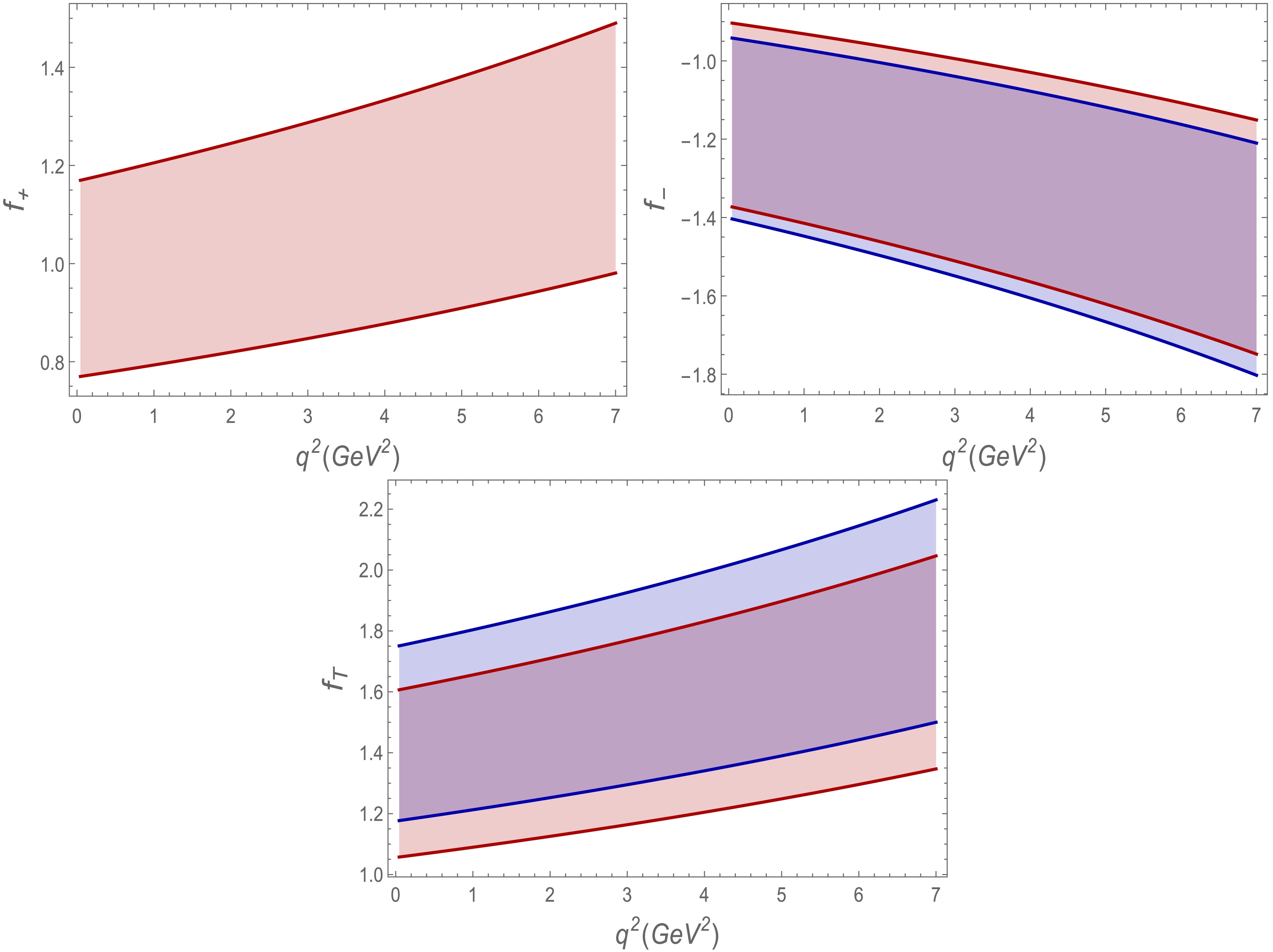
Figure 2. (color online) Form factors are plotted as a function of the momentum transfer
$ q^2 $ . The uncertainties are calculated at$ q^2=0 $ and then extrapolated as a function of$ q^2 $ . The red band represents the trend without symmetry-breaking effects, whereas the blue band incorporates the symmetry-breaking corrections.Using the uncertainties reported in [70−72], along with the other input parameters discussed above, we obtain bands as a function of
$ q^2 $ . In these plots, the red band represents the form factors without symmetry corrections, while the blue band corresponds to the same form factors after including the symmetry-breaking corrections. As can be observed from the plots,$ f_{-}(q^2) $ exhibits pronounced effects across the entire range of$ q^2 $ under consideration. For$ f_T(q^2) $ , normalized at$ \mu=m_b $ , the two bands overlap significantly over most of the$ q^2 $ region, indicating that the symmetry-breaking corrections are largely obscured by the various uncertainties. We emphasize again that the major uncertainty lies in the hard-spectator corrections due to the LCDA of the B meson. In the past, due to the lack of constraints on inverse moments, this uncertainty could rise as high as$ \pm 50{\text{%}} $ [41]. These uncertainties were constrained by the BABAR analysis of$ B \rightarrow \gamma \ell \nu_\ell $ [73] at small recoil and could be further improved by a similar BABAR analysis of the large-recoil radiative decay. This analysis was further refined in [74], since the former did not consider highly energetic photons and radiative/power corrections. In the context of [74], we expect larger uncertainties at large recoil than at small recoil. -
As discussed earlier, the corrections to the form factors receive contributions from vertex diagrams, with uncertainties originating from the renormalization scale of
$ \alpha_s $ . However, the hard-scattering corrections are subject to large theoretical uncertainties. These arise not only from the decay constants but also from the inverse moments defined in Eq. (36) and Eq. (37). It should be noted that the scale for the hard-scattering correction is$ (m_B\Lambda_{QCD})^{1/2} $ , and all quantities are evaluated at the scale$ \mu=1.47 $ GeV [41].Meson decay constants: Using the decay constants of the B and
$ K^{*}_0\left(1430\right) $ mesons,$ f_B= 0.195 \pm 0.01 $ GeV [67] and$ f_{K^{*}_0}=0.427 $ GeV [26, 68], respectively, we estimate the associated uncertainty in the hard-scattering corrections to be about ±15%.Light-cone distribution amplitudes: The light-cone distribution amplitudes (LCDAs) play a central role in the hard-scattering amplitudes. In particular, the inverse moment satisfies
$ \langle l_+^{-1} \rangle_+ \sim {\cal{O}}(1/\Lambda_{{\rm{QCD}}}) $ ; in the present analysis, we adopt the value for the B-meson moment$ \langle l_+^{-1} \rangle_+ = (0.35\,{\rm{GeV}})^{-1} $ . For the$ K_0^{*}(1430) $ meson, the LCDA is expanded in terms of Gegenbauer moments; the numerical value of the moment is$ \langle\bar{u}^{-1}\rangle = 1.422 $ , with details provided in Appendix A.Soft form factor: To determine the soft form factor
$ \xi_{K_0^{*}}(E_F) $ in the large-recoil region, required for evaluating the form factors$ f_+ $ ,$ f_- $ , and$ f_T $ , we employ results from light-cone sum rules (LCSR) for$ B \to K_0^{*} \ell^+ \ell^- $ decays [69, 70, 71]. We note that these studies do not include perturbative corrections. The value of$ \xi_{K_0^{*}} $ is extracted from the form factor$ f_+(q^2=0) $ using Eq. (25), yielding$ \xi_{K_0^{*}}(0) = 0.903 $ .The
$ q^2 $ -dependence of$ \xi_{K_0^{*}} $ is modeled using single- and double-pole parameterizations, following Ref. [70], over the kinematic range$ 0 \lt q^2 \lt (m_B - m_{K_0^{*}})^2 $ . The non-perturbative parameters$ a_i $ and$ b_i $ are determined within the LCSR framework in the low-$ q^2 $ region. The corresponding errors, together with the uncertainties in the soft form factor at$ q^2=0 $ and other input parameters, are propagated to obtain uncertainty bands for the form factors and related physical observables. Since the large-recoil symmetry relations are valid only for$ q^2 \ll m_B^2 $ , the analysis is restricted to$ q^2 \lesssim 7\,{\rm{GeV}}^2 $ . Using$ \alpha_s = 0.34 $ and the renormalization scale$ \mu = 1.47\,{\rm{GeV}} $ , the resulting form factors are computed and shown as functions of$ q^2 $ in Fig. 2.
Figure 2. (color online) Form factors are plotted as a function of the momentum transfer
$ q^2 $ . The uncertainties are calculated at$ q^2=0 $ and then extrapolated as a function of$ q^2 $ . The red band represents the trend without symmetry-breaking effects, whereas the blue band incorporates the symmetry-breaking corrections.Using the uncertainties reported in [69−71], along with the other input parameters discussed above, we obtain bands as a function of
$ q^2 $ . In these plots, the red band represents the form factors without symmetry corrections, while the blue band corresponds to the same form factors after including the symmetry-breaking corrections. As can be observed from the plots,$ f_{-}(q^2) $ exhibits pronounced effects across the entire range of$ q^2 $ under consideration. For$ f_T(q^2) $ , normalized at$ \mu=m_b $ , the two bands overlap significantly over most of the$ q^2 $ region, indicating that the symmetry-breaking corrections are largely obscured by the various uncertainties. We emphasize again that the major uncertainty lies in the hard-spectator corrections due to the LCDA of the B meson. In the past, due to the lack of constraints on inverse moments, this uncertainty could rise as high as$ \pm 50{\text{%}} $ [41]. These uncertainties were constrained by the BABAR analysis of$ B \rightarrow \gamma \ell \nu_\ell $ [72] at small recoil and could be further improved by a similar BABAR analysis of the large-recoil radiative decay. This analysis was further refined in [73], since the former did not consider highly energetic photons and radiative/power corrections. In the context of [73], we expect larger uncertainties at large recoil than at small recoil. -
It is valuable to assess the impact of the corrections to the form factors derived above by examining relevant observables. In this context, the decay amplitude and polarization asymmetries provide instructive examples. In this section, the effects of symmetry corrections to the form factors will be analyzed in the
$ B\to K_0^{*}\left(1430\right)\ell^+\ell^- $ decay within the SM. The decay of the B meson to a light scalar meson is induced by the flavor-changing neutral current transition$ b\to s\ell^+\ell^- $ . Within the SM, it is described by the effective Hamiltonian given in Eq. (1), whose contributions factorize into hadronic matrix elements. In general, however, not all contributions can be fully expressed in terms of form factors alone, because non-factorizable hard-scattering terms also arise (see, e.g., [42]). In the present framework, these non-factorizable effects are not included. Therefore, the decay amplitude can be summarized as$ {\cal{M}}_{B\to K_0^{*}\ell^+\ell^-}=-\frac{G_{\rm F}\alpha}{2\sqrt{2}\pi}V_{tb}V_{ts}^{*}[T_{\mu}^1(\bar{\ell}\gamma^\mu \ell)+T_{\mu}^2(\bar{\ell}\gamma^\mu\gamma_5 \ell)], $
(40) where
$ T_\mu^1 $ and$ T_\mu^2 $ denote the hadronic components of the decay amplitude and are defined as$ T_\mu^1=-C_9^{{\rm{eff}}}f_+(q^2)p_\mu+\frac{4m_b}{m_B+m_{K^{*}_0}}C_7^{{\rm{eff}}}f_T(q^2)p_\mu, $
(41) $ T_\mu^2=-C_{10} (f_+(q^2)p_\mu+f_-(q^2)q_\mu), $
(42) The differential decay rate:
The differential decay rate for this transition is given by Ref. [75]:
$ \begin{aligned}[b] \dfrac{{\rm d}\Gamma}{{\rm d}q^2}&\propto \Bigg[ \Big |-C_9^{{\rm{eff}}}f_+(q^2)p_\mu+\frac{4m_b}{m_B+m_{K^{*}_0}}C_7^{{\rm{eff}}}f_T(q^2)p_\mu \Big|^2\left(2m_l^2+q^2\right)\lambda + 12m_l^2q^4\Big|-C_{10}f_-(q^2)q_\mu\Big|^2 \\ &+ \Big|-C_{10} f_+(q^2)p_\mu\Big|^2\left\{(2m_l^2+q^2)(m_B^4-2m_B^2m^2_{K_0^{*}}-2q^2m^2_{K_0^{*}})+(m^2_{K_0^{*}}-q^2)^2+2m_l^2(m^4_{K_0^{*}}+10m^2_{K_0^{*}}+q^4)\right\} \\ &+12q^2m_l^2(m_B^2-m^2_{K_0^{*}}-q^2)\left|C_{10}\right|^2 p\cdot q\left(f_-(q^2)f_+^{*}\left(q^2\right)+f_-^{*}(q^2)f_+\left(q^2\right)\right) \Bigg]\;, \end{aligned} $
(43) where
$\begin{aligned}[b] \lambda=\;&\lambda(m^2_B,m^2_{K_0^{*}},q^2)=m_B^4+m^4_{K_0^{*}}+q^4\\&-2m_B^2m^2_{K_0^{*}}-2m^2_{K_0^{*}}q^2-2q^2m_B^2\;. \end{aligned}$
(44) The branching ratio is given as a function of momentum transfer
$ q^2 $ in Fig. 3. In the plots, the red curves represent the branching ratio at tree level, and the blue curves correspond to the branching ratio after including symmetry-breaking corrections. The band represents the uncertainties already discussed in the previous section. As can be observed, the inclusion of symmetry-breaking corrections in the form factors leads to only a small shift compared to the case without these corrections. The inset bar plots illustrate the effect of the form factors on observables across three different$ q^2 $ bins,$ (q^2_{{\rm{min}}}-2) $ ,$ (2-4) $ , and$ (4-7) $ in$ {\rm{GeV}}^2 $ .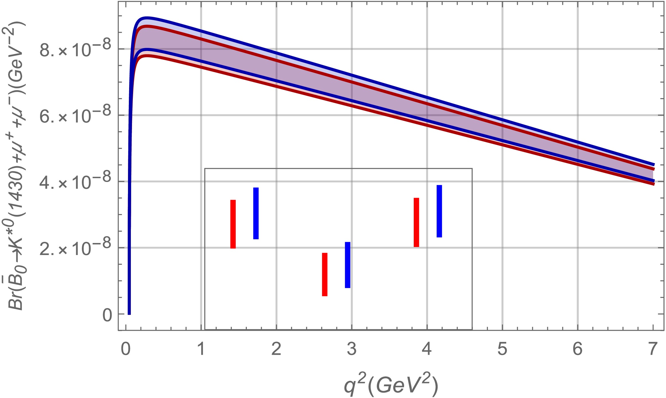
Figure 3. (color online) The branching ratio for
$ B\to K^{*}_0\mu^+\mu^- $ as a function of$ q^2 $ . -
It is valuable to assess the impact of the corrections to the form factors derived above by examining relevant observables. In this context, the decay amplitude and polarization asymmetries provide instructive examples. In this section, the effects of symmetry corrections to the form factors will be analyzed in the
$ B\to K_0^{*}\left(1430\right)\ell^+\ell^- $ decay within the SM. The decay of the B meson to a light scalar meson is induced by the flavor-changing neutral current transition$ b\to s\ell^+\ell^- $ . Within the SM, it is described by the effective Hamiltonian given in Eq. (1), whose contributions factorize into hadronic matrix elements. In general, however, not all contributions can be fully expressed in terms of form factors alone, because non-factorizable hard-scattering terms also arise (see, e.g., [42]). In the present framework, these non-factorizable effects are not included. Therefore, the decay amplitude can be summarized as$ {\cal{M}}_{B\to K_0^{*}\ell^+\ell^-}=-\frac{G_F\alpha}{2\sqrt{2}\pi}V_{tb}V_{ts}^{*}[T_{\mu}^1(\bar{\ell}\gamma^\mu \ell)+T_{\mu}^2(\bar{\ell}\gamma^\mu\gamma_5 \ell)] $
(40) where
$ T_\mu^1 $ and$ T_\mu^2 $ denote the hadronic components of the decay amplitude and are defined as$ T_\mu^1=-C_9^{{\rm{eff}}}f_+(q^2)p_\mu+\frac{4m_b}{m_B+m_{K^{*}_0}}C_7^{{\rm{eff}}}f_T(q^2)p_\mu $
(41) $ T_\mu^2=-C_{10} (f_+(q^2)p_\mu+f_-(q^2)q_\mu), $
(42) The differential decay rate:
The differential decay rate for this transition is given by Ref. [74]:
$ \begin{aligned}[b] \dfrac{d\Gamma}{dq^2}&\propto \Bigg[ \Big |-C_9^{{\rm{eff}}}f_+(q^2)p_\mu+\frac{4m_b}{m_B+m_{K^{*}_0}}C_7^{{\rm{eff}}}f_T(q^2)p_\mu \Big|^2\left(2m_l^2+q^2\right)\lambda + 12m_l^2q^4\Big|-C_{10}f_-(q^2)q_\mu\Big|^2 \\ &+ \Big|-C_{10} f_+(q^2)p_\mu\Big|^2\left\{(2m_l^2+q^2)(m_B^4-2m_B^2m^2_{K_0^{*}}-2q^2m^2_{K_0^{*}})+(m^2_{K_0^{*}}-q^2)^2+2m_l^2(m^4_{K_0^{*}}+10m^2_{K_0^{*}}+q^4)\right\} \\ &+12q^2m_l^2(m_B^2-m^2_{K_0^{*}}-q^2)\left|C_{10}\right|^2 p\cdot q\left(f_-(q^2)f_+^{*}\left(q^2\right)+f_-^{*}(q^2)f_+\left(q^2\right)\right) \Bigg]\;, \end{aligned} $
(43) where
$\begin{aligned}[b] \lambda=\;&\lambda(m^2_B,m^2_{K_0^{*}},q^2)=m_B^4+m^4_{K_0^{*}}+q^4\\&-2m_B^2m^2_{K_0^{*}}-2m^2_{K_0^{*}}q^2-2q^2m_B^2\;. \end{aligned}$
(44) The branching ratio is given as a function of momentum transfer
$ q^2 $ in Fig.(3). In the plots, the red curves represent the branching ratio at tree level, and the blue curves correspond to the branching ratio after including symmetry-breaking corrections. The band represents the uncertainties already discussed in the previous section. As can be observed, the inclusion of symmetry-breaking corrections in the form factors leads to only a small shift compared to the case without these corrections. The inset bar plots illustrate the effect of the form factors on observables across three different$ q^2 $ bins,$ (q^2_{{\rm{min}}}-2) $ ,$ (2-4) $ , and$ (4-7) $ in$ {\rm{GeV}}^2 $ .
Figure 3. (color online) The branching ratio for
$ B\to K^{*}_0\mu^+\mu^- $ as a function of$ q^2 $ . -
It is valuable to assess the impact of the corrections to the form factors derived above by examining relevant observables. In this context, the decay amplitude and polarization asymmetries provide instructive examples. In this section, the effects of symmetry corrections to the form factors will be analyzed in the
$ B\to K_0^{*}\left(1430\right)\ell^+\ell^- $ decay within the SM. The decay of the B meson to a light scalar meson is induced by the flavor-changing neutral current transition$ b\to s\ell^+\ell^- $ . Within the SM, it is described by the effective Hamiltonian given in Eq. (1), whose contributions factorize into hadronic matrix elements. In general, however, not all contributions can be fully expressed in terms of form factors alone, because non-factorizable hard-scattering terms also arise (see, e.g., [42]). In the present framework, these non-factorizable effects are not included. Therefore, the decay amplitude can be summarized as$ {\cal{M}}_{B\to K_0^{*}\ell^+\ell^-}=-\frac{G_{\rm F}\alpha}{2\sqrt{2}\pi}V_{tb}V_{ts}^{*}[T_{\mu}^1(\bar{\ell}\gamma^\mu \ell)+T_{\mu}^2(\bar{\ell}\gamma^\mu\gamma_5 \ell)], $
(40) where
$ T_\mu^1 $ and$ T_\mu^2 $ denote the hadronic components of the decay amplitude and are defined as$ T_\mu^1=-C_9^{{\rm{eff}}}f_+(q^2)p_\mu+\frac{4m_b}{m_B+m_{K^{*}_0}}C_7^{{\rm{eff}}}f_T(q^2)p_\mu, $
(41) $ T_\mu^2=-C_{10} (f_+(q^2)p_\mu+f_-(q^2)q_\mu), $
(42) The differential decay rate:
The differential decay rate for this transition is given by Ref. [75]:
$ \begin{aligned}[b] \dfrac{{\rm d}\Gamma}{{\rm d}q^2}&\propto \Bigg[ \Big |-C_9^{{\rm{eff}}}f_+(q^2)p_\mu+\frac{4m_b}{m_B+m_{K^{*}_0}}C_7^{{\rm{eff}}}f_T(q^2)p_\mu \Big|^2\left(2m_l^2+q^2\right)\lambda + 12m_l^2q^4\Big|-C_{10}f_-(q^2)q_\mu\Big|^2 \\ &+ \Big|-C_{10} f_+(q^2)p_\mu\Big|^2\left\{(2m_l^2+q^2)(m_B^4-2m_B^2m^2_{K_0^{*}}-2q^2m^2_{K_0^{*}})+(m^2_{K_0^{*}}-q^2)^2+2m_l^2(m^4_{K_0^{*}}+10m^2_{K_0^{*}}+q^4)\right\} \\ &+12q^2m_l^2(m_B^2-m^2_{K_0^{*}}-q^2)\left|C_{10}\right|^2 p\cdot q\left(f_-(q^2)f_+^{*}\left(q^2\right)+f_-^{*}(q^2)f_+\left(q^2\right)\right) \Bigg]\;, \end{aligned} $
(43) where
$\begin{aligned}[b] \lambda=\;&\lambda(m^2_B,m^2_{K_0^{*}},q^2)=m_B^4+m^4_{K_0^{*}}+q^4\\&-2m_B^2m^2_{K_0^{*}}-2m^2_{K_0^{*}}q^2-2q^2m_B^2\;. \end{aligned}$
(44) The branching ratio is given as a function of momentum transfer
$ q^2 $ in Fig. 3. In the plots, the red curves represent the branching ratio at tree level, and the blue curves correspond to the branching ratio after including symmetry-breaking corrections. The band represents the uncertainties already discussed in the previous section. As can be observed, the inclusion of symmetry-breaking corrections in the form factors leads to only a small shift compared to the case without these corrections. The inset bar plots illustrate the effect of the form factors on observables across three different$ q^2 $ bins,$ (q^2_{{\rm{min}}}-2) $ ,$ (2-4) $ , and$ (4-7) $ in$ {\rm{GeV}}^2 $ .
Figure 3. (color online) The branching ratio for
$ B\to K^{*}_0\mu^+\mu^- $ as a function of$ q^2 $ . -
In this decay, the lepton pair exhibits longitudinal, normal, and transverse polarization components. The longitudinal polarization is given by:
$ \begin{aligned}[b] P_L(q^2)& \propto \left(1-\frac{4m_l^2}{q^2}\right)\Bigg[(-C_9^{{\rm{eff}}}f_+(q^2)p_\mu+\frac{4m_b}{m_B+m_{K^{*}_0}}C_7^{{\rm{eff}}}f_T(q^2)p_\mu))(-C_{10} f_+(q^2)p^\mu)^{*} \\ &+(-C_9^{{\rm{eff}}}f_+(q^2)p_\mu+\frac{4m_b}{m_B+m_{K^{*}_0}}C_7^{{\rm{eff}}}f_T(q^2)p_\mu)^{*}(-C_{10} f_+(q^2)p^\mu)\Bigg] \end{aligned} $
(45) The normal lepton polarization in the decay
$ B\to K^{*}_0\ell^+\ell^- $ is given by the following expression:$ \begin{aligned}[b] P_N(q^2) \propto \left(1 - \frac{4 m_l^2}{q^2}\right) \Bigg[ &\left( - C_9^{{\rm{eff}}} f_+(q^2)p_\mu + \frac{4 m_b}{m_B + m_{K_0^{*}}} C_7^{{\rm{eff}}} f_T(q^2)p_\mu \right) \left(- C_{10} f_+(q^2)p^\mu\right)^{*} \\ &+ \left( - C_9^{{\rm{eff}}} f_+(q^2)p_\mu + \frac{4 m_b}{m_B + m_{K_0^{*}}} C_7^{{\rm{eff}}} f_T(q^2)p_\mu \right)^{*} \left(- C_{10} f_+(q^2)p^\mu\right) \\ &- 2 q^2 \left( - C_9^{{\rm{eff}}} f_+(q^2)p_\mu + \frac{4 m_b}{m_B + m_{K_0^{*}}} C_7^{{\rm{eff}}} f_T(q^2)p_\mu \right)^{*} \left(- C_{10} f_-(q^2) q^\mu\right) \\ &+ \left( - C_9^{{\rm{eff}}} f_+(q^2)p_\mu + \frac{4 m_b}{m_B + m_{K_0^{*}}} C_7^{{\rm{eff}}} f_T(q^2)p_\mu \right) \left(- C_{10} f_-(q^2) q^\mu\right)^{*} \Bigg] \end{aligned} $
(46) Fig.(4) illustrates the behavior of
$ P_L $ and$ P_N $ , where the color coding is the same as that used for the branching ratio. The plots overlap in the low-$ q^2 $ region, whereas a significant deviation is observed in the lepton polarization in the intermediate-$ q^2 $ region.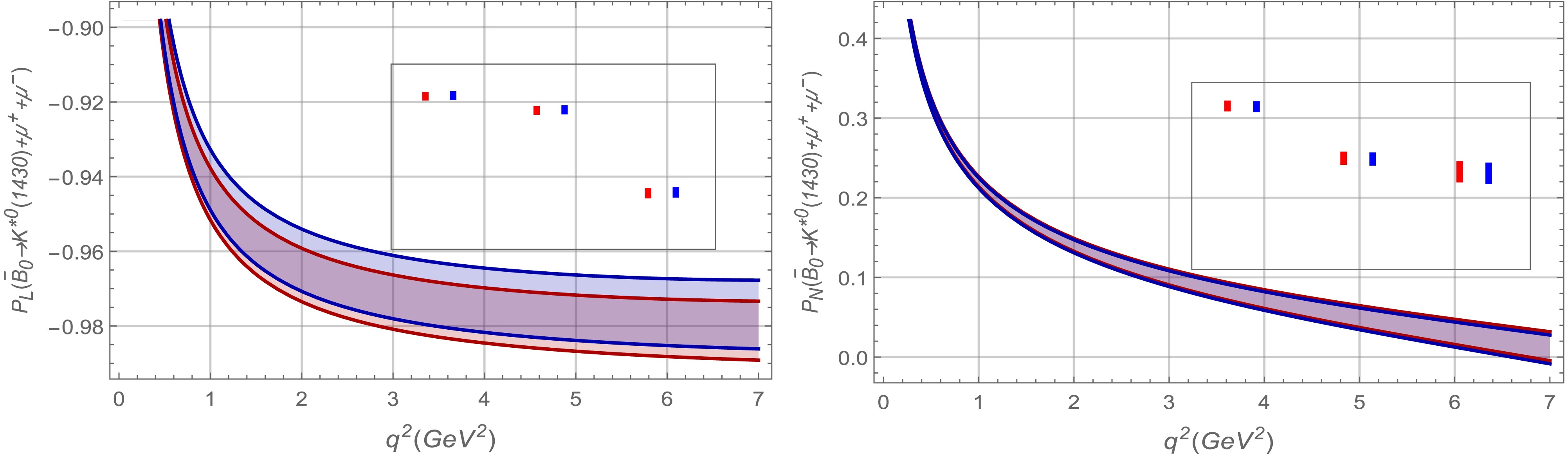
Figure 4. (color online) Lepton polarization in the decay
$ B\to K^{*}_0\mu^+\mu^- $ as a function of$ q^2 $ . -
In this decay, the lepton pair exhibits longitudinal, normal, and transverse polarization components. The longitudinal polarization is given by:
$ \begin{aligned}[b] P_L(q^2) \; \propto \; & \left(1-\frac{4m_l^2}{q^2}\right)\Bigg[(-C_9^{{\rm{eff}}}f_+(q^2)p_\mu+\frac{4m_b}{m_B+m_{K^{*}_0}}C_7^{{\rm{eff}}}f_T(q^2)p_\mu))(-C_{10} f_+(q^2)p^\mu)^{*} \\ &+(-C_9^{{\rm{eff}}}f_+(q^2)p_\mu+\frac{4m_b}{m_B+m_{K^{*}_0}}C_7^{{\rm{eff}}}f_T(q^2)p_\mu)^{*}(-C_{10} f_+(q^2)p^\mu)\Bigg]. \end{aligned} $
(45) The normal lepton polarization in the decay
$ B\to K^{*}_0\ell^+\ell^- $ is given by the following expression:$ \begin{aligned}[b] P_N(q^2) \propto \left(1 - \frac{4 m_l^2}{q^2}\right) \Bigg[ &\left( - C_9^{{\rm{eff}}} f_+(q^2)p_\mu + \frac{4 m_b}{m_B + m_{K_0^{*}}} C_7^{{\rm{eff}}} f_T(q^2)p_\mu \right) \left(- C_{10} f_+(q^2)p^\mu\right)^{*} \\ &+ \left( - C_9^{{\rm{eff}}} f_+(q^2)p_\mu + \frac{4 m_b}{m_B + m_{K_0^{*}}} C_7^{{\rm{eff}}} f_T(q^2)p_\mu \right)^{*} \left(- C_{10} f_+(q^2)p^\mu\right) \\ &- 2 q^2 \left( - C_9^{{\rm{eff}}} f_+(q^2)p_\mu + \frac{4 m_b}{m_B + m_{K_0^{*}}} C_7^{{\rm{eff}}} f_T(q^2)p_\mu \right)^{*} \left(- C_{10} f_-(q^2) q^\mu\right) \\ &+ \left( - C_9^{{\rm{eff}}} f_+(q^2)p_\mu + \frac{4 m_b}{m_B + m_{K_0^{*}}} C_7^{{\rm{eff}}} f_T(q^2)p_\mu \right) \left(- C_{10} f_-(q^2) q^\mu\right)^{*} \Bigg]. \end{aligned} $
(46) Figure 4 illustrates the behavior of
$ P_L $ and$ P_N $ , where the color coding is the same as that used for the branching ratio. The plots overlap in the low-$ q^2 $ region, whereas a significant deviation is observed in the lepton polarization in the intermediate-$ q^2 $ region.
Figure 4. (color online) Lepton polarization in the decay
$ B\to K^{*}_0\mu^+\mu^- $ as a function of$ q^2 $ . -
In this work, we have computed the symmetry-breaking corrections to the form factors governing the rare decay
$ B \to K_0^{*} \ell^+ \ell^- $ at one-loop order. These corrections become particularly relevant in the large-recoil region,$ q^2 \sim 1 $ –$ 7\,{\rm{GeV}}^2 $ . The structure of these effects is described within the QCD factorization framework [58], where short-distance contributions from heavy degrees of freedom, as well as hard virtual corrections, are treated perturbatively, while long-distance dynamics associated with light quarks and gluons are encoded in nonperturbative hadronic matrix elements parameterized by form factors.In the heavy-quark and large-recoil limit, the three independent form factors
$ f_+(q^2) $ ,$ f_-(q^2) $ , and$ f_T(q^2) $ relevant for$ B \to K_0^{*} \ell^+ \ell^- $ transitions reduce to a single universal soft form factor$ \xi_{K_0^{*}} $ . Corrections to these symmetry relations arise from hard-gluon interactions and can be systematically classified into vertex and hard-spectator contributions. The vertex corrections are computed at$ {\cal{O}}(\alpha_s) $ by matching the effective theory onto full QCD, while the hard-spectator contributions are evaluated using the light-cone distribution amplitudes of the participating mesons.Our numerical analysis shows that the inclusion of symmetry-breaking corrections leads to deviations of about
$ 4{\text{%}} $ in$ f_-(q^2) $ and$ 10{\text{%}} $ in$ f_T(q^2) $ relative to their symmetry-limit values. These modified form-factor relations at large recoil have a noticeable impact on phenomenological observables. In particular, we find that the branching ratio receives a correction of approximately$ 3{\text{%}} $ , while the normal lepton polarization asymmetry$ P_N $ is also affected at the level of$ \sim 3{\text{%}} $ . The longitudinal polarization$ P_L $ remains largely unchanged, whereas the transverse polarization$ P_T $ does not receive any significant contribution from symmetry-breaking effects in the present framework. We note that the uncertainties from the meson decay constants are$ \pm 15{\text{%}} $ . These parameters enter through subleading contributions and via convolution integrals in the hard-scattering kernel. Thus, the dominant contributions are governed by form-factor terms, while the dependence on$ f_B $ and$ \langle l_+^{-1} \rangle_+ $ is either power-suppressed or enters in combination with other hadronic quantities inside convolution integrals. Consequently, despite the relatively large uncertainties in the input parameters, their net impact on the final observables remains at the level of a few percent. Therefore, due to the relatively small magnitude of these symmetry-breaking corrections, any sizable deviations observed from the SM predictions in these decays would clearly hint at potential new-physics effects.In the future, lattice QCD calculations are expected to play a crucial role in reducing the uncertainties arising from hadronic inputs. Thus, more precise lattice determinations of
$ f_B $ and improved constraints on the low moments of the B-meson distribution amplitude, either directly or via related HQET matrix elements, would significantly reduce the parametric uncertainties in the hard-scattering contributions. This would allow a more precise isolation of subleading power corrections in$ B \rightarrow K^{*}_0(1430) $ transitions. On the experimental side, advances in the precision of measurements of various observables and LFU-sensitive ratios will further tighten the constraints on form factors, helping to disentangle hadronic effects from possible NP contributions. Specifically, improved data on branching ratios and angular observables will reduce the allowed range of input parameters. As a result, future progress, both theoretically and experimentally, will substantially reduce these uncertainties and enhance the sensitivity to such subleading effects. -
The light-cone distribution amplitudes of the scalar meson,
$ \phi_S(u) $ at twist-2 and$ \phi^s_S(u) $ and$ \phi^\sigma_S(u) $ at twist-3, are given by:$ \begin{aligned}[b]& \langle S(p)|\,\bar{q}_2(z_2)\gamma_\mu q_1(z_1)\,|0\rangle\\=\;& f_S p_\mu \int_0^1 du\; e^{i(up\cdot z_2 + \bar{u}p\cdot z_1)}\, \phi_S(u), \\ &\langle S(p)|\,\bar{q}_2(z_2) q_1(z_1)\,|0\rangle \\=\;&\bar f_S m_S \int_0^1 du\; e^{i(up\cdot z_2 + \bar{u}p\cdot z_1)}\, \phi_S^s(u), \\ &\langle S(p)|\,\bar{q}_2(z_2)\sigma_{\mu\nu} q_1(z_1)\,|0\rangle \\=\;& -\bar f_Sm_S (p_\mu z_\nu - p_\nu z_\mu) \int_0^1 du\; e^{i(up\cdot z_2 + \bar{u}p\cdot z_1)}\, \frac{\phi_S^\sigma(u)}{6}. \end{aligned} $
(A1) The LCDAs in Eq. (A1) can be combined into a single matrix element as
$ \begin{aligned}[b]&\langle S(p)|\,\bar{q}_{2\beta}(z_2)\,q_{1\alpha}(z_1)\,|0\rangle = \frac{\bar f_S}{4} \int_0^1 du\; e^{i(up\cdot z_2 + \bar{u}p\cdot z_1)} \\&\quad\times\left\{ \not{p}\,\phi_S(u) + m_S \left( \phi_S^s(u) - \sigma_{\mu\nu} p^\mu z^\nu \frac{\phi_S^\sigma(u)}{6} \right) \right\}_{\alpha\beta} \end{aligned} $
(A2) The general expression for the twist-2 LCDA of scalar mesons is given by
$ \phi_S(u,\mu)=6u\bar{u}\left[B_0(\mu)+\sum^\infty_{n=1} B_n(\mu)C^{3/2}_n\left( 2u-1 \right)\right] $
(A3) where
$ \bar{u}=1-u $ and$ S={K^{*}_0} $ ; see [24, 75]. The normalization condition gives$ B_0=\mu_S^{-1} $ . The coefficients$ B_n(\mu) $ are the Gegenbauer moments, with$ C^{3/2}(2u-1) $ denoting the Gegenbauer polynomials, both depending on the renormalization scale μ. Due to the asymmetric nature of the scalar-meson LCDA, only odd Gegenbauer moments contribute, leading to the vanishing of even moments, i.e.,$ B_2 = B_4 = 0 $ . Further details can be found in [69]. The first few Gegenbauer polynomials are given by$ \begin{aligned}[b]&C_1^{3/2}(2u-1)=3(2u-1), \\& C_2^{3/2}(2u-1)=\frac{3}{2}\left[5(2u-1)^2-1\right], \;\; \cdots \end{aligned}$
(A4) Neglecting higher-order contributions and retaining only the leading nontrivial term, Eq. (A3) reduces to
$ \phi_{K^{*}_0}(u,\mu)=6u\bar{u}[B_0(\mu)+ B_1(\mu) C_1^{3/2}(2u-1)]\;. $
(A5) This is the final truncated form of the LCDA for the
$ K^{*}_0 $ meson. The leading-twist moment of the scalar meson is then obtained by integrating the expression above, as given in Eq. (37). -
The light-cone distribution amplitudes of the scalar meson,
$ \phi_S(u) $ at twist-2 and$ \phi^s_S(u) $ and$ \phi^\sigma_S(u) $ at twist-3, are given by:$ \begin{aligned}[b]& \langle S(p)|\,\bar{q}_2(z_2)\gamma_\mu q_1(z_1)\,|0\rangle\\=\;& f_S p_\mu \int_0^1 {\rm d}u\; {\rm e}^{{\rm i}(up\cdot z_2 + \bar{u}p\cdot z_1)}\, \phi_S(u), \\ &\langle S(p)|\,\bar{q}_2(z_2) q_1(z_1)\,|0\rangle \\=\;&\bar f_S m_S \int_0^1 {\rm d}u\; {\rm e}^{{\rm i}(up\cdot z_2 + \bar{u}p\cdot z_1)}\, \phi_S^s(u), \\ &\langle S(p)|\,\bar{q}_2(z_2)\sigma_{\mu\nu} q_1(z_1)\,|0\rangle \\=\;& -\bar f_Sm_S (p_\mu z_\nu - p_\nu z_\mu) \int_0^1 {\rm d}u\; {\rm e}^{{\rm i}(up\cdot z_2 + \bar{u}p\cdot z_1)}\, \frac{\phi_S^\sigma(u)}{6}. \end{aligned} $
(A1) The LCDAs in Eq. (A1) can be combined into a single matrix element as
$ \begin{aligned}[b]&\langle S(p)|\,\bar{q}_{2\beta}(z_2)\,q_{1\alpha}(z_1)\,|0\rangle = \frac{\bar f_S}{4} \int_0^1 {\rm d}u\; {\rm e}^{{\rm i}(up\cdot z_2 + \bar{u}p\cdot z_1)} \\&\quad\times\left\{ \not{p}\,\phi_S(u) + m_S \left( \phi_S^s(u) - \sigma_{\mu\nu} p^\mu z^\nu \frac{\phi_S^\sigma(u)}{6} \right) \right\}_{\alpha\beta}. \end{aligned} $
(A2) The general expression for the twist-2 LCDA of scalar mesons is given by
$ \phi_S(u,\mu)=6u\bar{u}\left[B_0(\mu)+\sum^\infty_{n=1} B_n(\mu)C^{3/2}_n\left( 2u-1 \right)\right], $
(A3) where
$ \bar{u}=1-u $ and$ S={K^{*}_0} $ ; see [24, 67]. The normalization condition gives$ B_0=\mu_S^{-1} $ . The coefficients$ B_n(\mu) $ are the Gegenbauer moments, with$ C^{3/2}(2u-1) $ denoting the Gegenbauer polynomials, both depending on the renormalization scale μ. Due to the asymmetric nature of the scalar-meson LCDA, only odd Gegenbauer moments contribute, leading to the vanishing of even moments, i.e.,$ B_2 = B_4 = 0 $ . Further details can be found in [70]. The first few Gegenbauer polynomials are given by$ \begin{aligned}[b]&C_1^{3/2}(2u-1)=3(2u-1), \\& C_2^{3/2}(2u-1)=\frac{3}{2}\left[5(2u-1)^2-1\right], \;\; \cdots \end{aligned}$
(A4) Neglecting higher-order contributions and retaining only the leading nontrivial term, Eq. (A3) reduces to
$ \phi_{K^{*}_0}(u,\mu)=6u\bar{u}[B_0(\mu)+ B_1(\mu) C_1^{3/2}(2u-1)]\;. $
(A5) This is the final truncated form of the LCDA for the
$ K^{*}_0 $ meson. The leading-twist moment of the scalar meson is then obtained by integrating the expression above, as given in Eq. (37). -
In this section, we evaluate the B-meson projection operator as defined in Eq. (32). The derivation starts from the two-particle light-cone matrix element in coordinate space. We then introduce the distribution amplitudes
$ \phi_\pm^B(t) $ via the Lorentz decomposition of the corresponding light-cone matrix element, which can be expressed as:$\begin{aligned}[b]& \langle0|\bar{q}_\beta(z)P(z,0)b_\alpha(0)|\bar{B}(p\rangle)\\=\;&-\frac{if_Bm_B}{4}\Bigg[ \frac{1+\not{v}}{2}\{2\phi_+^B(t)+\frac{\phi_-^B(t)-\phi_+^B(t)}{t}\not{z}\}\gamma_5\Bigg]_{\alpha\beta} .\end{aligned} $
(B1) We now impose the light-cone condition
$ z^2 = 0 $ and define$ t = v \cdot z $ . The momentum of the B-meson is given by$ p = m_B v $ , where$ m_B $ denotes the mass of the B-meson. The path-ordered exponential can then be written as$ P(z_2,z_1)=P{\rm{exp}}\Bigg(ig_s\int^{z_1}_{z_2}dz^\mu A_\mu(z)\Bigg). $
(B2) The momentum-space projector in Eq. (B1) is most compatible with Lorentz invariance and with the heavy-quark limit. The first factor is chosen such that, for
$ z=0 $ , it yields$ \langle0|\bar{q}_\beta[\gamma^\mu\gamma_5]_{\beta\alpha} b_\alpha|\bar{B}(p\rangle)=if_Bm_Bv^\mu, $
(B3) Assume
$ \phi_+^B(t=0)=\phi_-^B(t=0)=1 $ . Here,$ \phi_+^B $ denotes the leading-twist term, while$ \phi_-^B $ denotes the subleading-twist term. In Eq. (B1), let$ M(z) $ denote the matrix element and$ A(z) $ ($ A(l) $ ) the hard-scattering amplitude in momentum space; then Eq. (32) can be obtained by using the identity$\begin{aligned}[b] \int d^4zM(z)A(z)=\;&\int\frac{d^4l}{(2\pi)^4}A(l)\int d^4ze^{-ilz}M(z)\\\equiv\;&\int^\infty_0dl_+M^BA(l)\Bigg|_{l=\frac{l_+}{2}n_+},\end{aligned} $
(B4) with the components of
$ l^\mu $ decomposed as$ l^\mu=\frac{l_+}{2}n^\mu_++\frac{l_-}{2}n^\mu_-+l^\mu_\perp $
(B5) The coordinate functions
$ \phi_\pm^B(t) $ in momentum space are expressed as:$ \phi_\pm^B(t)\equiv\int^\infty_0dwe^{-iwt}\phi_\pm^B(w). $
(B6) In the heavy-quark limit, the hard-scattering amplitude
$ A(l) $ for a light meson moving in the$ n_- $ direction does not depend on$ l_- $ . Therefore,$ A(l)=A^0(l_+)+l^\mu_\perp A^1_\mu(l_+)+O(1/m_B). $
(B7) and, after ignoring the
$ l_- $ term, the derivative is$ \frac{\partial}{\partial l_\mu}=n_-^\mu\frac{\partial}{\partial l_\mu}+\frac{\partial}{\partial l_{\perp\mu}}. $
(B8) Combining Eqs. (B6) and (B8) into Eq. (B4), we obtain a momentum-space projector, namely a two-particle light-cone projector involving only the b quark and a light spectator quark, valid when the three-particle contribution is neglected. It is given by
${ M^B_{\beta\alpha}=-\dfrac{if_Bm_B}{4}\left[ \dfrac{1+\not{v}}{2} \left\{ \phi_+^B(w)\,\not{n}_+ + \phi_-^B(w) \left( \not{n}_- - l_+\,\gamma^\nu_\perp \dfrac{\partial}{\partial l^\nu_\perp} \right) \right\} \gamma_5 \right]_{\beta\alpha} \Bigg|_{\,l=\frac{l_+}{2}n_+}. }$
(B9) -
In this section, we evaluate the B-meson projection operator as defined in Eq. (32). The derivation starts from the two-particle light-cone matrix element in coordinate space. We then introduce the distribution amplitudes
$ \phi_\pm^B(t) $ via the Lorentz decomposition of the corresponding light-cone matrix element, which can be expressed as:$\begin{aligned}[b]& \langle0|\bar{q}_\beta(z)P(z,0)b_\alpha(0)|\bar{B}(p\rangle)\\=\;&-\frac{{\rm i} f_Bm_B}{4}\Bigg[ \frac{1+\not{\,v}}{2} \left\{2\phi_+^B(t)+\frac{\phi_-^B(t)-\phi_+^B(t)}{t}\not{\,z}\right\}\gamma_5\Bigg]_{\alpha\beta} .\end{aligned} $
(B1) We now impose the light-cone condition
$ z^2 = 0 $ and define$ t = v \cdot z $ . The momentum of the B-meson is given by$ p = m_B v $ , where$ m_B $ denotes the mass of the B-meson. The path-ordered exponential can then be written as$ P(z_2,z_1)=P{\rm{exp}}\Bigg({\rm i} g_s\int^{z_1}_{z_2}{\rm d}z^\mu A_\mu(z)\Bigg). $
(B2) The momentum-space projector in Eq. (B1) is most compatible with Lorentz invariance and with the heavy-quark limit. The first factor is chosen such that, for
$ z=0 $ , it yields$ \langle0|\bar{q}_\beta[\gamma^\mu\gamma_5]_{\beta\alpha} b_\alpha|\bar{B}(p\rangle)={\rm i}f_Bm_Bv^\mu, $
(B3) Assume
$ \phi_+^B(t=0)=\phi_-^B(t=0)=1 $ . Here,$ \phi_+^B $ denotes the leading-twist term, while$ \phi_-^B $ denotes the subleading-twist term. In Eq. (B1), let$ M(z) $ denote the matrix element and$ A(z) $ ($ A(l) $ ) the hard-scattering amplitude in momentum space; then Eq. (32) can be obtained by using the identity$\begin{aligned}[b] \int {\rm d}^4zM(z)A(z)=\int\frac{{\rm d}^4l}{(2\pi)^4}A(l)\int {\rm d}^4z {\rm e}^{-{\rm i}lz}M(z)\end{aligned} $
$\begin{aligned}[b] \equiv\int^\infty_0{\rm d}l_+M^BA(l)\Bigg|_{l=\frac{l_+}{2}n_+},\end{aligned} $
(B4) with the components of
$ l^\mu $ decomposed as$ l^\mu=\frac{l_+}{2}n^\mu_++\frac{l_-}{2}n^\mu_-+l^\mu_\perp .$
(B5) The coordinate functions
$ \phi_\pm^B(t) $ in momentum space are expressed as:$ \phi_\pm^B(t)\equiv\int^\infty_0{\rm d}w{\rm e}^{-{\rm i}wt}\phi_\pm^B(w). $
(B6) In the heavy-quark limit, the hard-scattering amplitude
$ A(l) $ for a light meson moving in the$ n_- $ direction does not depend on$ l_- $ . Therefore,$ A(l)=A^0(l_+)+l^\mu_\perp A^1_\mu(l_+)+O(1/m_B). $
(B7) After ignoring the
$ l_- $ term, the derivative is$ \frac{\partial}{\partial l_\mu}=n_-^\mu\frac{\partial}{\partial l_\mu}+\frac{\partial}{\partial l_{\perp\mu}}. $
(B8) Combining Eqs. (B6) and (B8) into Eq. (B4), we obtain a momentum-space projector, namely a two-particle light-cone projector involving only the b quark and a light spectator quark, valid when the three-particle contribution is neglected. It is given by
$\begin{aligned}[b] M^B_{\beta\alpha} =\; &-\dfrac{{\rm i}f_Bm_B}{4}\bigg[ \dfrac{1+\not{\,v}}{2} \bigg\{ \phi_+^B(w)\,\not{\,n}_+ \\ & + \phi_-^B(w) \left( \not{\,n}_- - l_+\,\gamma^\nu_\perp \dfrac{\partial}{\partial l^\nu_\perp} \right) \bigg\} \gamma_5 \bigg]_{\beta\alpha} \Bigg|_{\,l=\frac{l_+}{2}n_+}. \end{aligned}$
(B9)
Symmetry-breaking effects on form factors and observables in B → K0*(1430)μ+μ– decay
- Received Date: 2026-03-19
- Available Online: 2026-07-15
Abstract: In the heavy-quark and large-energy limits, symmetry relations reduce the number of independent form factors governing heavy-to-light B-meson decays. Exploiting these relations, the form factors can be parametrized while systematically incorporating symmetry-breaking corrections from perturbative QCD. Using vertex renormalization together with light-cone distribution amplitudes, we compute the vertex and hard-spectator contributions for the $B \to K_0^{*}(1430)$ transition. We then analyze the impact of these form factors on physical observables, including the branching ratio and lepton polarization asymmetries $(P_L, P_N)$, in $B \to K_0^{*}(1430)\mu^+\mu^-$. Our results indicate that perturbative corrections induce modest shifts of ~ 3% in both the branching ratio and the normal lepton polarization asymmetry. Consequently, any significant deviation observed experimentally from these predictions would provide a clear signal of potential New Physics effects.


 DownLoad: