


 Abstract
 HTML
HTML Reference
 Related
 PDF
PDF


-
The conventional quark model provides a useful framework for classifying hadrons made of quarks and/or antiquarks, in which mesons are described as bound states of a quark and an antiquark (
$ q\bar{q} $ ), and baryons as three-quark systems (qqq). This model, though conceptually simple, has achieved remarkable success in explaining the properties and spectrum of hadrons, leveraging constituent quark dynamics to capture essential features of hadron structure. Quantum chromodynamics (QCD), the foundational theory of strong interactions, also predicts the existence of "so-called" exotic hadrons with more complicated constituent structures beyond the conventional quark model. These exotic states can provide rich information about the non-perturbative aspects of QCD and serve as valuable probes for understanding its complex phenomena.Among the various exotic candidates, hadrons with quantum numbers that defy the conventional quark model are considered strong evidence for the existence of exotic hadrons. Specifically, a hybrid state is composed of a constituent quark and antiquark, together with a constituent gluon, and can naturally exhibit quantum numbers beyond the conventional
$ q\bar{q} $ scenario. For instance, for the lowest hybrid systems with zero orbital angular momentum, the quantum numbers$ J^{P(C)} = 0^{-(+)}/1^{-(\pm)}/2^{-(+)} $ can be accessed, where$ J^{PC}=1^{-+} $ cannot be accessed by the conventional$ q\bar{q} $ configuration. This particular class of hadrons has attracted significant attention from both experiment and theory, driving continued explorations of hadron structures and the underlying dynamics. In 2009, the COMPASS Collaboration reported the$ J^{PC}=1^{-+} $ candidate with isospin 1, i.e.$ \pi_1(1600) $ , through the partial wave analysis [1]. Their analysis also clarified that the evidence for$ \pi_1(1400) $ seems to be caused by interference from$ \pi_1(1600) $ . In 2022, the BESIII Collaboration reported the first observation of the$ 1^{-+} $ isoscalar hybrid candidate$ \eta_1(1855) $ in a partial wave analysis of$ J/\psi \to \gamma \eta_1(1855) \to \gamma \eta \eta' $ [2, 3]. The mass and total decay width of this state are$ (1855\pm9^{+6}_{-1})\; {\rm MeV} $ and$ (188\pm18^{+3}_{-8})\; {\rm MeV} $ , respectively. This breakthrough provides a valuable opportunity to gain deeper insight into these mysterious hadron species and has stimulated considerable theoretical interest [4−16]. In fact, an immediate question concerning hybrid states is that of their partners. For instance, in the light quark sector, one would expect the existence of a flavor nonet$ q\bar{q}\tilde{g} $ . An immediate investigation of the hybrid nonet after the observation of$ \eta_1(1855) $ can be found in Ref. [4]. Historically, experimental efforts in the search for hybrid states can be found in the literature [17−22]. Comprehensive reviews of the relevant issues can be found in Refs. [23, 24].The possible existence of the hybrid nonet has strong support from lattice QCD simulations [25, 26]. With
$ \pi_1(1600) $ assigned as the isovector state and$ \eta_1(1855) $ as one of the isoscalar states, two pieces are still missing from the jigsaw puzzle. Namely, these are the isospin$ 1/2 $ partner with strangeness$ \pm 1 $ and the other isoscalar state$ \eta_1' $ . In Ref. [4], possible solutions for the nonet spectrum based on the Gell-Mann–Okubo mass relation were discussed. An interesting feature of the isospin$ 1/2 $ partners is that they do not have a fixed C-parity. With$ J^P=1^- $ , such a hybrid state has the same quantum numbers as the$ q\bar{q} $ state. Thus, it may mix with the$ 1^- $ states in the same mass regime.The strange
$ I=1/2 $ partner can be assigned to$ K^*(1680) $ , which is the only strange vector meson found in the vicinity of the mass region$ 1.6-1.9 $ GeV [27]. Given that$ \pi_1(1600) $ is the isovector state of the lowest$ 1^{-+} $ hybrid,$ K^*(1410) $ is too light to be its strange partner. Actually,$ K^*(1410) $ also appears to be too light for a$ 2^3S_1 $ state, taking into account its isovector partner$ \rho(1450) $ [27]. In Ref. [28], it was suggested that the low mass of$ K^*(1410) $ might be due to the presence of additional hybrid admixtures.It is possible to assign
$ K^*(1680) $ as the$ 1^3D_1 $ vector in the strange sector. However, the relative branching fraction of$ K^*(1680)^- $ to$ K^-\eta $ and$ K^-\pi^0 $ measured by the Belle Collaboration,$ 0.11\pm0.02({\rm stat})^{+0.06}_{-0.04}({\rm syst})\pm0.54({\cal B}_{\rm PDG}) $ [29], does not seem to be consistent with the theoretical predictions$ (\approx 1) $ under the assumption that$ K^*(1680) $ is a pure$ 1^3D_1 $ state [30, 31]. In Ref. [30], the relationship between the$ K^*(1410) $ and$ K^*(1680) $ mesons and the D-wave spectrum were investigated, and it was also shown that$ K^*(1680) $ cannot be a pure$ ^3D_1 $ state.The above issues leave open the possibility that
$ K^*(1680) $ could be a candidate for the strange hybrid or a mixed state between the$ q\bar{q} $ and hybrid configurations [4].In this work, we explore the possibility that
$ K^*(1680) $ is the strange hybrid of the$ 1^{-(+)} $ nonet. At the same time, it should be recognized that the hybrid$ K^* $ can mix with the conventional vector state. To clarify this, we also consider the impact of$ q\bar{q} $ mixing with the hybrid on the decay of$ K^*(1680) $ . The idea is that, if$ K^*(1680) $ is assumed to be a conventional$ q\bar{q} $ state in the quark model, its two-body decays into different channels can be reasonably described by the quark pair creation model (QPC) [32−37], which is also known as the$ ^3P_0 $ ($ n^{2S+1}L_J $ ) model. Since the QPC model has been broadly applied to various decay processes and has proven successful [38−44], significant deviations from the QPC model expectations may indicate nontrivial mechanisms or structures different from the$ q\bar{q} $ scenario. It is reasonable to assume that, as the strange hybrid of the$ J^{P(C)}=1^{-(+)} $ nonet, the two-body hadronic decays of$ K^*(1680) $ should differ from those of a$ q\bar{q} $ meson. We therefore investigate whether such a possibility exists.While there have been various phenomenological studies of hybrid states in the literature [45−48], the flux-tube (FT) model [49] provides a dynamical connection between the decay mechanism of a hybrid state and that of a
$ q\bar{q} $ meson in the QPC model. For the decay of a hybrid in the FT model, the collinear mode describing the motion of the constituent gluon along the direction between q and$ \bar{q} $ can be regarded as equivalent to the QPC model if multi-soft-gluon exchanges are included in the decay. In contrast, the transverse mode of gluon motion should manifest itself as a mechanism different from the QPC model, since contributions from the gluon degrees of freedom can affect the quantum numbers in addition to those of the$ q\bar{q} $ subsystem. In this sense, we can parametrize the transitions involving both the$ q\bar{q} $ and hybrid configurations and examine whether the present experimental data provide evidence for the hybrid configuration.The remainder of the paper is organized as follows: In Sec. II, we present our theoretical framework. In Sec. III, numerical results are given. Comparisons with the available experimental data and discussions of the underlying mechanisms are presented. A brief summary is given in Sec. IV.
-
The conventional quark model provides a useful framework for classifying hadrons made of quarks and/or antiquarks, in which mesons are described as bound states of a quark and an antiquark (
$ q\bar{q} $ ), and baryons as three-quark systems (qqq). This model, though conceptually simple, has achieved remarkable success in explaining the properties and spectrum of hadrons, leveraging constituent quark dynamics to capture essential features of hadron structure. Quantum chromodynamics (QCD), the foundational theory of strong interactions, also predicts the existence of "so-called" exotic hadrons with more complicated constituent structures beyond the conventional quark model. These exotic states can provide rich information about the non-perturbative aspects of QCD and serve as valuable probes for understanding its complex phenomena.Among the various exotic candidates, hadrons with quantum numbers that defy the conventional quark model are considered strong evidence for the existence of exotic hadrons. Specifically, a hybrid state is composed of a constituent quark and antiquark, together with a constituent gluon, and can naturally exhibit quantum numbers beyond the conventional
$ q\bar{q} $ scenario. For instance, for the lowest hybrid systems with zero orbital angular momentum, the quantum numbers$ J^{P(C)} = 0^{-(+)}/1^{-(\pm)}/2^{-(+)} $ can be accessed, where$ J^{PC}=1^{-+} $ cannot be accessed by the conventional$ q\bar{q} $ configuration. This particular class of hadrons has attracted significant attention from both experiment and theory, driving continued explorations of hadron structures and the underlying dynamics. In 2009, the COMPASS Collaboration reported the$ J^{PC}=1^{-+} $ candidate with isospin 1, i.e.$ \pi_1(1600) $ , through the partial wave analysis [1]. Their analysis also clarified that the evidence for$ \pi_1(1400) $ seems to be caused by interference from$ \pi_1(1600) $ . In 2022, the BESIII Collaboration reported the first observation of the$ 1^{-+} $ isoscalar hybrid candidate$ \eta_1(1855) $ in a partial wave analysis of$ J/\psi \to \gamma \eta_1(1855) \to \gamma \eta \eta' $ [2, 3]. The mass and total decay width of this state are$ (1855\pm9^{+6}_{-1})\; {\rm MeV} $ and$ (188\pm18^{+3}_{-8})\; {\rm MeV} $ , respectively. This breakthrough provides a valuable opportunity to gain deeper insight into these mysterious hadron species and has stimulated considerable theoretical interest [4−16]. In fact, an immediate question concerning hybrid states is that of their partners. For instance, in the light quark sector, one would expect the existence of a flavor nonet$ q\bar{q}\tilde{g} $ . An immediate investigation of the hybrid nonet after the observation of$ \eta_1(1855) $ can be found in Ref. [4]. Historically, experimental efforts in the search for hybrid states can be found in the literature [17−22]. Comprehensive reviews of the relevant issues can be found in Refs. [23, 24].The possible existence of the hybrid nonet has strong support from lattice QCD simulations [25, 26]. With
$ \pi_1(1600) $ assigned as the isovector state and$ \eta_1(1855) $ as one of the isoscalar states, two pieces are still missing from the jigsaw puzzle. Namely, these are the isospin$ 1/2 $ partner with strangeness$ \pm 1 $ and the other isoscalar state$ \eta_1' $ . In Ref. [4], possible solutions for the nonet spectrum based on the Gell-Mann–Okubo mass relation were discussed. An interesting feature of the isospin$ 1/2 $ partners is that they do not have a fixed C-parity. With$ J^P=1^- $ , such a hybrid state has the same quantum numbers as the$ q\bar{q} $ state. Thus, it may mix with the$ 1^- $ states in the same mass regime.The strange
$ I=1/2 $ partner can be assigned to$ K^*(1680) $ , which is the only strange vector meson found in the vicinity of the mass region$ 1.6-1.9 $ GeV [27]. Given that$ \pi_1(1600) $ is the isovector state of the lowest$ 1^{-+} $ hybrid,$ K^*(1410) $ is too light to be its strange partner. Actually,$ K^*(1410) $ also appears to be too light for a$ 2^3S_1 $ state, taking into account its isovector partner$ \rho(1450) $ [27]. In Ref. [28], it was suggested that the low mass of$ K^*(1410) $ might be due to the presence of additional hybrid admixtures.It is possible to assign
$ K^*(1680) $ as the$ 1^3D_1 $ vector in the strange sector. However, the relative branching fraction of$ K^*(1680)^- $ to$ K^-\eta $ and$ K^-\pi^0 $ measured by the Belle Collaboration,$ 0.11\pm0.02({\rm stat})^{+0.06}_{-0.04}({\rm syst})\pm0.54({\cal B}_{\rm PDG}) $ [29], does not seem to be consistent with the theoretical predictions$ (\approx 1) $ under the assumption that$ K^*(1680) $ is a pure$ 1^3D_1 $ state [30, 31]. In Ref. [30], the relationship between the$ K^*(1410) $ and$ K^*(1680) $ mesons and the D-wave spectrum were investigated, and it was also shown that$ K^*(1680) $ cannot be a pure$ ^3D_1 $ state.The above issues leave open the possibility that
$ K^*(1680) $ could be a candidate for the strange hybrid or a mixed state between the$ q\bar{q} $ and hybrid configurations [4].In this work, we explore the possibility that
$ K^*(1680) $ is the strange hybrid of the$ 1^{-(+)} $ nonet. At the same time, it should be recognized that the hybrid$ K^* $ can mix with the conventional vector state. To clarify this, we also consider the impact of$ q\bar{q} $ mixing with the hybrid on the decay of$ K^*(1680) $ . The idea is that, if$ K^*(1680) $ is assumed to be a conventional$ q\bar{q} $ state in the quark model, its two-body decays into different channels can be reasonably described by the quark pair creation model (QPC) [32−37], which is also known as the$ ^3P_0 $ ($ n^{2S+1}L_J $ ) model. Since the QPC model has been broadly applied to various decay processes and has proven successful [38−44], significant deviations from the QPC model expectations may indicate nontrivial mechanisms or structures different from the$ q\bar{q} $ scenario. It is reasonable to assume that, as the strange hybrid of the$ J^{P(C)}=1^{-(+)} $ nonet, the two-body hadronic decays of$ K^*(1680) $ should differ from those of a$ q\bar{q} $ meson. We therefore investigate whether such a possibility exists.While there have been various phenomenological studies of hybrid states in the literature [45−48], the flux-tube (FT) model [49] provides a dynamical connection between the decay mechanism of a hybrid state and that of a
$ q\bar{q} $ meson in the QPC model. For the decay of a hybrid in the FT model, the collinear mode describing the motion of the constituent gluon along the direction between q and$ \bar{q} $ can be regarded as equivalent to the QPC model if multi-soft-gluon exchanges are included in the decay. In contrast, the transverse mode of gluon motion should manifest itself as a mechanism different from the QPC model, since contributions from the gluon degrees of freedom can affect the quantum numbers in addition to those of the$ q\bar{q} $ subsystem. In this sense, we can parametrize the transitions involving both the$ q\bar{q} $ and hybrid configurations and examine whether the present experimental data provide evidence for the hybrid configuration.The remainder of the paper is organized as follows: In Sec. II, we present our theoretical framework. In Sec. III, numerical results are given. Comparisons with the available experimental data and discussions of the underlying mechanisms are presented. A brief summary is given in Sec. IV.
-
The conventional quark model provides a useful framework for classifying hadrons made of quarks and/or antiquarks, in which mesons are described as bound states of a quark and an antiquark (
$ q\bar{q} $ ), and baryons as three-quark systems (qqq). This model, though conceptually simple, has achieved remarkable success in explaining the properties and spectrum of hadrons, leveraging constituent quark dynamics to capture essential features of hadron structure. Quantum chromodynamics (QCD), the foundational theory of strong interactions, also predicts the existence of "so-called" exotic hadrons with more complicated constituent structures beyond the conventional quark model. These exotic states can provide rich information about the non-perturbative aspects of QCD and serve as valuable probes for understanding its complex phenomena.Among the various exotic candidates, hadrons with quantum numbers that defy the conventional quark model are considered strong evidence for the existence of exotic hadrons. Specifically, a hybrid state is composed of a constituent quark and antiquark, together with a constituent gluon, and can naturally exhibit quantum numbers beyond the conventional
$ q\bar{q} $ scenario. For instance, for the lowest hybrid systems with zero orbital angular momentum, the quantum numbers$ J^{P(C)} = 0^{-(+)}/1^{-(\pm)}/2^{-(+)} $ can be accessed, where$ J^{PC}=1^{-+} $ cannot be accessed by the conventional$ q\bar{q} $ configuration. This particular class of hadrons has attracted significant attention from both experiment and theory, driving continued explorations of hadron structures and the underlying dynamics. In 2009, the COMPASS Collaboration reported the$ J^{PC}=1^{-+} $ candidate with isospin 1, i.e.$ \pi_1(1600) $ , through the partial wave analysis [1]. Their analysis also clarified that the evidence for$ \pi_1(1400) $ seems to be caused by interference from$ \pi_1(1600) $ . In 2022, the BESIII Collaboration reported the first observation of the$ 1^{-+} $ isoscalar hybrid candidate$ \eta_1(1855) $ in a partial wave analysis of$ J/\psi \to \gamma \eta_1(1855) \to \gamma \eta \eta' $ [2, 3]. The mass and total decay width of this state are$ (1855\pm9^{+6}_{-1})\; {\rm MeV} $ and$ (188\pm18^{+3}_{-8})\; {\rm MeV} $ , respectively. This breakthrough provides a valuable opportunity to gain deeper insight into these mysterious hadron species and has stimulated considerable theoretical interest [4−16]. In fact, an immediate question concerning hybrid states is that of their partners. For instance, in the light quark sector, one would expect the existence of a flavor nonet$ q\bar{q}\tilde{g} $ . An immediate investigation of the hybrid nonet after the observation of$ \eta_1(1855) $ can be found in Ref. [4]. Historically, experimental efforts in the search for hybrid states can be found in the literature [17−22]. Comprehensive reviews of the relevant issues can be found in Refs. [23, 24].The possible existence of the hybrid nonet has strong support from lattice QCD simulations [25, 26]. With
$ \pi_1(1600) $ assigned as the isovector state and$ \eta_1(1855) $ as one of the isoscalar states, two pieces are still missing from the jigsaw puzzle. Namely, these are the isospin$ 1/2 $ partner with strangeness$ \pm 1 $ and the other isoscalar state$ \eta_1' $ . In Ref. [4], possible solutions for the nonet spectrum based on the Gell-Mann–Okubo mass relation were discussed. An interesting feature of the isospin$ 1/2 $ partners is that they do not have a fixed C-parity. With$ J^P=1^- $ , such a hybrid state has the same quantum numbers as the$ q\bar{q} $ state. Thus, it may mix with the$ 1^- $ states in the same mass regime.The strange
$ I=1/2 $ partner can be assigned to$ K^*(1680) $ , which is the only strange vector meson found in the vicinity of the mass region$ 1.6-1.9 $ GeV [27]. Given that$ \pi_1(1600) $ is the isovector state of the lowest$ 1^{-+} $ hybrid,$ K^*(1410) $ is too light to be its strange partner. Actually,$ K^*(1410) $ also appears to be too light for a$ 2^3S_1 $ state, taking into account its isovector partner$ \rho(1450) $ [27]. In Ref. [28], it was suggested that the low mass of$ K^*(1410) $ might be due to the presence of additional hybrid admixtures.It is possible to assign
$ K^*(1680) $ as the$ 1^3D_1 $ vector in the strange sector. However, the relative branching fraction of$ K^*(1680)^- $ to$ K^-\eta $ and$ K^-\pi^0 $ measured by the Belle Collaboration,$ 0.11\pm0.02({\rm stat})^{+0.06}_{-0.04}({\rm syst})\pm0.54({\cal B}_{\rm PDG}) $ [29], does not seem to be consistent with the theoretical predictions$ (\approx 1) $ under the assumption that$ K^*(1680) $ is a pure$ 1^3D_1 $ state [30, 31]. In Ref. [30], the relationship between the$ K^*(1410) $ and$ K^*(1680) $ mesons and the D-wave spectrum were investigated, and it was also shown that$ K^*(1680) $ cannot be a pure$ ^3D_1 $ state.The above issues leave open the possibility that
$ K^*(1680) $ could be a candidate for the strange hybrid or a mixed state between the$ q\bar{q} $ and hybrid configurations [4].In this work, we explore the possibility that
$ K^*(1680) $ is the strange hybrid of the$ 1^{-(+)} $ nonet. At the same time, it should be recognized that the hybrid$ K^* $ can mix with the conventional vector state. To clarify this, we also consider the impact of$ q\bar{q} $ mixing with the hybrid on the decay of$ K^*(1680) $ . The idea is that, if$ K^*(1680) $ is assumed to be a conventional$ q\bar{q} $ state in the quark model, its two-body decays into different channels can be reasonably described by the quark pair creation model (QPC) [32−37], which is also known as the$ ^3P_0 $ ($ n^{2S+1}L_J $ ) model. Since the QPC model has been broadly applied to various decay processes and has proven successful [38−44], significant deviations from the QPC model expectations may indicate nontrivial mechanisms or structures different from the$ q\bar{q} $ scenario. It is reasonable to assume that, as the strange hybrid of the$ J^{P(C)}=1^{-(+)} $ nonet, the two-body hadronic decays of$ K^*(1680) $ should differ from those of a$ q\bar{q} $ meson. We therefore investigate whether such a possibility exists.While there have been various phenomenological studies of hybrid states in the literature [45−48], the flux-tube (FT) model [49] provides a dynamical connection between the decay mechanism of a hybrid state and that of a
$ q\bar{q} $ meson in the QPC model. For the decay of a hybrid in the FT model, the collinear mode describing the motion of the constituent gluon along the direction between q and$ \bar{q} $ can be regarded as equivalent to the QPC model if multi-soft-gluon exchanges are included in the decay. In contrast, the transverse mode of gluon motion should manifest itself as a mechanism different from the QPC model, since contributions from the gluon degrees of freedom can affect the quantum numbers in addition to those of the$ q\bar{q} $ subsystem. In this sense, we can parametrize the transitions involving both the$ q\bar{q} $ and hybrid configurations and examine whether the present experimental data provide evidence for the hybrid configuration.The remainder of the paper is organized as follows: In Sec. II, we present our theoretical framework. In Sec. III, numerical results are given. Comparisons with the available experimental data and discussions of the underlying mechanisms are presented. A brief summary is given in Sec. IV.
-
The conventional quark model provides a useful framework for classifying hadrons made of quarks and/or antiquarks, in which mesons are described as bound states of a quark and an antiquark (
$ q\bar{q} $ ), and baryons as three-quark systems (qqq). This model, though conceptually simple, has achieved remarkable success in explaining the properties and spectrum of hadrons, leveraging constituent quark dynamics to capture essential features of hadron structure. Quantum chromodynamics (QCD), the foundational theory of strong interactions, also predicts the existence of "so-called" exotic hadrons with more complicated constituent structures beyond the conventional quark model. These exotic states can provide rich information about the non-perturbative aspects of QCD and serve as valuable probes for understanding its complex phenomena.Among the various exotic candidates, hadrons with quantum numbers that defy the conventional quark model are considered strong evidence for the existence of exotic hadrons. Specifically, a hybrid state is composed of a constituent quark and antiquark, together with a constituent gluon, and can naturally exhibit quantum numbers beyond the conventional
$ q\bar{q} $ scenario. For instance, for the lowest hybrid systems with zero orbital angular momentum, the quantum numbers$ J^{P(C)} = 0^{-(+)}/1^{-(\pm)}/2^{-(+)} $ can be accessed, where$ J^{PC}=1^{-+} $ cannot be accessed by the conventional$ q\bar{q} $ configuration. This particular class of hadrons has attracted significant attention from both experiment and theory, driving continued explorations of hadron structures and the underlying dynamics. In 2009, the COMPASS Collaboration reported the$ J^{PC}=1^{-+} $ candidate with isospin 1, i.e.$ \pi_1(1600) $ , through the partial wave analysis [1]. Their analysis also clarified that the evidence for$ \pi_1(1400) $ seems to be caused by interference from$ \pi_1(1600) $ . In 2022, the BESIII Collaboration reported the first observation of the$ 1^{-+} $ isoscalar hybrid candidate$ \eta_1(1855) $ in a partial wave analysis of$ J/\psi \to \gamma \eta_1(1855) \to \gamma \eta \eta' $ [2, 3]. The mass and total decay width of this state are$ (1855\pm9^{+6}_{-1})\; {\rm MeV} $ and$ (188\pm18^{+3}_{-8})\; {\rm MeV} $ , respectively. This breakthrough provides a valuable opportunity to gain deeper insight into these mysterious hadron species and has stimulated considerable theoretical interest [4−16]. In fact, an immediate question concerning hybrid states is that of their partners. For instance, in the light quark sector, one would expect the existence of a flavor nonet$ q\bar{q}\tilde{g} $ . An immediate investigation of the hybrid nonet after the observation of$ \eta_1(1855) $ can be found in Ref. [4]. Historically, experimental efforts in the search for hybrid states can be found in the literature [17−22]. Comprehensive reviews of the relevant issues can be found in Refs. [23, 24].The possible existence of the hybrid nonet has strong support from lattice QCD simulations [25, 26]. With
$ \pi_1(1600) $ assigned as the isovector state and$ \eta_1(1855) $ as one of the isoscalar states, two pieces are still missing from the jigsaw puzzle. Namely, these are the isospin$ 1/2 $ partner with strangeness$ \pm 1 $ and the other isoscalar state$ \eta_1' $ . In Ref. [4], possible solutions for the nonet spectrum based on the Gell-Mann–Okubo mass relation were discussed. An interesting feature of the isospin$ 1/2 $ partners is that they do not have a fixed C-parity. With$ J^P=1^- $ , such a hybrid state has the same quantum numbers as the$ q\bar{q} $ state. Thus, it may mix with the$ 1^- $ states in the same mass regime.The strange
$ I=1/2 $ partner can be assigned to$ K^*(1680) $ , which is the only strange vector meson found in the vicinity of the mass region$ 1.6-1.9 $ GeV [27]. Given that$ \pi_1(1600) $ is the isovector state of the lowest$ 1^{-+} $ hybrid,$ K^*(1410) $ is too light to be its strange partner. Actually,$ K^*(1410) $ also appears to be too light for a$ 2^3S_1 $ state, taking into account its isovector partner$ \rho(1450) $ [27]. In Ref. [28], it was suggested that the low mass of$ K^*(1410) $ might be due to the presence of additional hybrid admixtures.It is possible to assign
$ K^*(1680) $ as the$ 1^3D_1 $ vector in the strange sector. However, the relative branching fraction of$ K^*(1680)^- $ to$ K^-\eta $ and$ K^-\pi^0 $ measured by the Belle Collaboration,$ 0.11\pm0.02({\rm stat})^{+0.06}_{-0.04}({\rm syst})\pm0.54({\cal B}_{\rm PDG}) $ [29], does not seem to be consistent with the theoretical predictions$ (\approx 1) $ under the assumption that$ K^*(1680) $ is a pure$ 1^3D_1 $ state [30, 31]. In Ref. [30], the relationship between the$ K^*(1410) $ and$ K^*(1680) $ mesons and the D-wave spectrum were investigated, and it was also shown that$ K^*(1680) $ cannot be a pure$ ^3D_1 $ state.The above issues leave open the possibility that
$ K^*(1680) $ could be a candidate for the strange hybrid or a mixed state between the$ q\bar{q} $ and hybrid configurations [4].In this work, we explore the possibility that
$ K^*(1680) $ is the strange hybrid of the$ 1^{-(+)} $ nonet. At the same time, it should be recognized that the hybrid$ K^* $ can mix with the conventional vector state. To clarify this, we also consider the impact of$ q\bar{q} $ mixing with the hybrid on the decay of$ K^*(1680) $ . The idea is that, if$ K^*(1680) $ is assumed to be a conventional$ q\bar{q} $ state in the quark model, its two-body decays into different channels can be reasonably described by the quark pair creation model (QPC) [32−37], which is also known as the$ ^3P_0 $ ($ n^{2S+1}L_J $ ) model. Since the QPC model has been broadly applied to various decay processes and has proven successful [38−44], significant deviations from the QPC model expectations may indicate nontrivial mechanisms or structures different from the$ q\bar{q} $ scenario. It is reasonable to assume that, as the strange hybrid of the$ J^{P(C)}=1^{-(+)} $ nonet, the two-body hadronic decays of$ K^*(1680) $ should differ from those of a$ q\bar{q} $ meson. We therefore investigate whether such a possibility exists.While there have been various phenomenological studies of hybrid states in the literature [45−48], the flux-tube (FT) model [49] provides a dynamical connection between the decay mechanism of a hybrid state and that of a
$ q\bar{q} $ meson in the QPC model. For the decay of a hybrid in the FT model, the collinear mode describing the motion of the constituent gluon along the direction between q and$ \bar{q} $ can be regarded as equivalent to the QPC model if multi-soft-gluon exchanges are included in the decay. In contrast, the transverse mode of gluon motion should manifest itself as a mechanism different from the QPC model, since contributions from the gluon degrees of freedom can affect the quantum numbers in addition to those of the$ q\bar{q} $ subsystem. In this sense, we can parametrize the transitions involving both the$ q\bar{q} $ and hybrid configurations and examine whether the present experimental data provide evidence for the hybrid configuration.The remainder of the paper is organized as follows: In Sec. II, we present our theoretical framework. In Sec. III, numerical results are given. Comparisons with the available experimental data and discussions of the underlying mechanisms are presented. A brief summary is given in Sec. IV.
-
Our strategy for studying the properties of
$ K^*(1680) $ is based on the following considerations: (i) As mentioned earlier, the two-body decays of an initial$ q\bar{q} $ state can be reasonably described within the QPC model. This allows us to investigate the$ q\bar{q} $ scenario for$ K^*(1680)\to PP $ and VP as a conventional$ q\bar{q} $ state and to establish relations among these decay channels via SU(3) flavor symmetry. By assigning$ K^*(1680) $ as either the first radial excitation state$ 2^3S_1 $ or the orbital excitation state$ 1^3D_1 $ , we will examine whether it can be described within the$ q\bar{q} $ scenario. (ii) By introducing the hybrid scenario, we will also investigate the decay patterns of the initial hybrid$ K^*(1680)\to PP $ and VP, with both the collinear and transverse modes considered. (iii) We then consider$ K^*(1680) $ as a mixed state of a conventional$ q\bar{q} $ state and a hybrid. The mixing angle will be fitted through an overall description of all the two-body decay channels of$ K^*(1680)\to PP $ and VP.At the hadronic level, the decay of an initial vector meson into PP and VP can be described by effective Lagrangians. With V and P denoting the ground-state vector and pseudoscalar mesons, respectively, SU(3) flavor symmetry allows us to establish connections among all the PP and VP decay channels. The following effective Lagrangians are adopted:
$ \begin{aligned} {\cal{L}}_{VPP}&= {\rm i} g_{VPP} {\rm Tr} [(P\partial_{\mu}P- \partial_{\mu}P P)V^{\mu}], \end{aligned} $
(1) $ \begin{aligned} {\cal{L}}_{VVP}&= \frac{1}{m_V} g_{VVP}\epsilon_{\alpha\beta\mu\nu} {\rm Tr} [\partial^\alpha V^\mu \partial^\beta V^\nu P], \end{aligned} $
(2) where
$ g_{VPP} $ and$ g_{VVP} $ are dimensionless coupling strengths. Here, V and P denote the vector and pseudoscalar fields of the ground-state SU(3) nonet, respectively, and take the following forms$ \begin{aligned} P & = \left( \begin{array}{*{20}{c}} {\dfrac{{\sin {\alpha _P}\eta' + \cos {\alpha _P}\eta + {\pi ^0}}}{{\sqrt 2 }}}&{{\pi ^ + }}&{{K^ + }}\\ \pi^- &{\dfrac{{\sin {\alpha _P}\eta' + \cos {\alpha _P}\eta - {\pi ^0}}}{{\sqrt 2 }}}&{{K^0}}\\ {{K^ - }}&{{{\bar K}^0}}&{\cos {\alpha_P}\eta' - \sin {\alpha _P}\eta } \end{array} \right), \end{aligned} $
(3) and
$ \begin{aligned} V &= \left( \begin{array}{*{20}{c}} \dfrac{\omega + \rho ^0}{\sqrt 2}&\rho^+&K^{*+}\\ \rho^-&\dfrac{\omega - \rho ^0}{\sqrt 2}&K^{*0}\\ {{K^{* - }}}&{{{\bar K}^{*0}}}&\phi \end{array} \right). \end{aligned} $
(4) In the vector sector, ideal mixing between
$ \omega=(u\bar u + d\bar d)/ \sqrt 2 $ and$ \phi = s\bar s $ is adopted. As for η and$ \eta' $ , they can be expressed in the quark-flavor basis as$ \eta = \cos \alpha_P n\bar n - \sin\alpha_P s\bar s $ and$ \eta' = \sin \alpha_P n\bar n + \cos\alpha_P s\bar s $ , where$ n\bar n \equiv (u\bar u + d\bar d)/\sqrt2 $ , and the mixing angle$ \alpha_P \equiv \arctan\sqrt 2 + \theta_p $ , with$ \theta_p $ being the flavor singlet-octet mixing angle. For the two-body hadronic decays, most of the$ K^*(1680) \to PP $ and VP decay channels are kinematically allowed. We focus on the PP and VP decay channels, taking into account the experimental situation. The hadronic-level transition amplitudes in the effective Lagrangian approach (ELA) are as follows:$ \begin{aligned} {\rm i}{\cal{M}}_{VPP}^{{\rm{ELA}}}&= {\rm i} g_{VPP}(p_B-p_C)_{\mu}\epsilon_A^{\mu} = {\rm i} g_{VPP} 2 |{\boldsymbol{p}}_B|, \end{aligned} $
(5) $ \begin{aligned} {\rm i}{\cal{M}}_{VVP}^{{\rm{ELA}}}&= \frac{1}{m_A} {\rm i} g_{VVP}\epsilon_{\alpha\beta\mu\nu} p_A^{\alpha}p_B^{\beta}\epsilon_A^{\mu}{\epsilon_B^{\nu}}^* = {\rm i} g_{VVP}m_A |{\boldsymbol{p}}_B|. \end{aligned} $
(6) The coupling constants defined above can receive contributions from the decay of the conventional
$ q\bar{q} $ component via the QPC model and from the decay of the hybrid component via the FT model.As discussed earlier, the FT model actually contains the QPC model. Its collinear mode shares dynamics similar to those of the QPC model in the decay. Since we consider only the decays of a fixed set of processes, namely
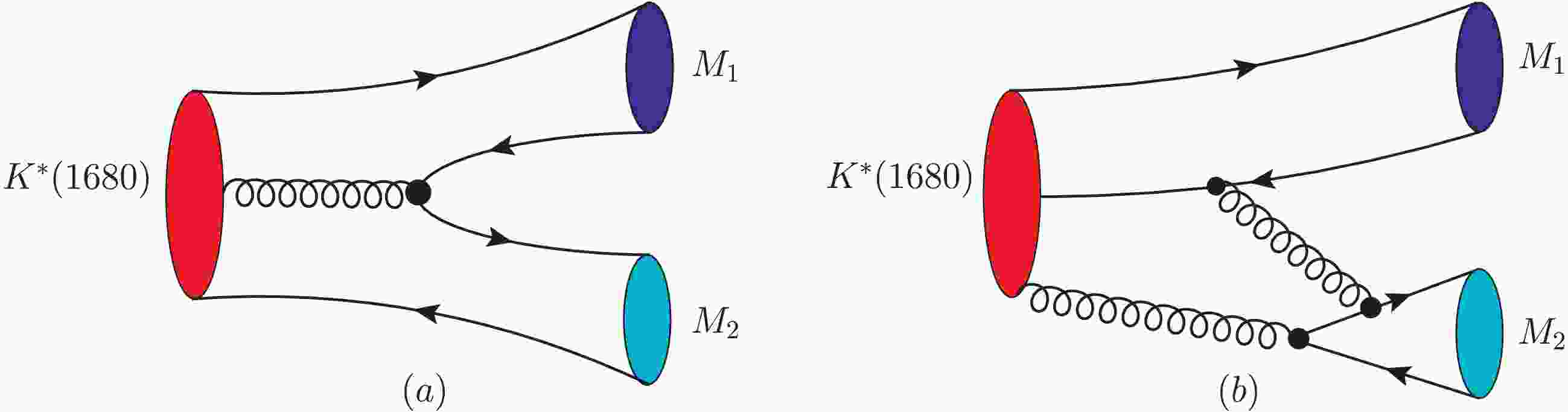
$ K^*(1680)\to VP $ and PP, we assume that the collinear mode can be described by the QPC model. Meanwhile, the transverse mode is driven by a different mechanism. These are two independent mechanisms for hybrid decays and are illustrated in Fig. 1 (a) and (b), respectively. At the quark level, Fig. 1 (a) dominates the collinear mode and describes the breaking of the flux-tube string through the creation of a$ q\bar{q} $ pair that combines with the initial quark and antiquark. With multi-gluon exchanges during hadronization, Fig. 1 (a) behaves similarly to the QPC transition. This allows us to evaluate the coupling of the collinear-mode decay using the QPC model and to unify these two mechanisms within the same framework.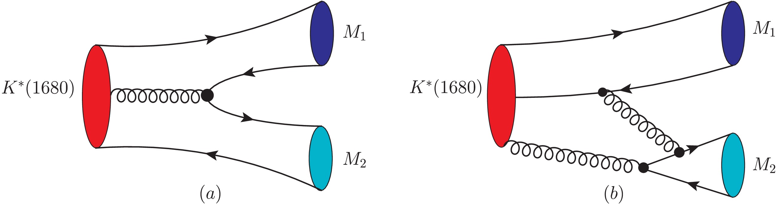
Figure 1. (color online) Schematic illustrations of the two-body hadronic decays of hybrid states. Panel (a) is dominated by the collinear mode, while panel (b) is dominated by the transverse mode.
The hybrid decay via the transverse mode dominates the process shown in Fig. 1 (b). The quark pair created by the transverse mode causes the initial quark-antiquark pair to recoil through the transverse flux motion. Then, with a soft gluon exchange that neutralizes the color of the recoiled
$ q\bar{q} $ pair, the process shown in Fig. 1 (b) plays a crucial and unique role in decay channels involving the production of flavor-singlet hadrons. For conventional$ q\bar{q} $ decays, a process similar to that shown in Fig. 1 (b) may also occur. However, it is usually suppressed by the Okubo-Zweig-Iizuka (OZI) rule. In contrast, in the decay of a hybrid, Fig. 1 (b) is not necessarily suppressed [50].With the above considerations, we can define the transition amplitude for a
$ 1^{-+} $ hybrid of$ q\bar{q}\tilde{g} $ decaying into two conventional mesons, PP and VP, as follows [4]$ \begin{aligned}[b] &{\cal{M}}_a^{VPP}= \langle(q_1\bar{q_4})_{P} (q_3\bar{q_2})_{P}|\hat V_C|q_1\bar{q_2}\tilde{g}\rangle \equiv g_{1}^{VPP}|{\boldsymbol{p}}_B |, \\ &{\cal{M}}_b^{VPP}= \langle(q_1\bar{q_2})_{P} (q_3\bar{q_4})_{P}|\hat V_T|q_1\bar{q_2}\tilde{g}\rangle \equiv g_{2}^{VPP}|{\boldsymbol{p}}_B |, \\ &{\cal{M}}_a^{VVP}= \langle(q_1\bar{q_4})_{P(V)} (q_3\bar{q_2})_{V(P)}|\hat V_C|q_1\bar{q_2}\tilde{g}\rangle \equiv g_{1}^{VVP}|{\boldsymbol{p}}_B |, \\ &{\cal{M}}_b^{VVP}= \langle(q_1\bar{q_2})_{P(V)} (q_3\bar{q_4})_{V(P)}|\hat V_T|q_1\bar{q_2}\tilde{g}\rangle \equiv g_{2}^{VVP}|{\boldsymbol{p}}_B |, \end{aligned} $
(7) where
$ {\cal{M}}_a $ and$ {\cal{M}}_b $ are the amplitudes corresponding to the collinear and transverse flux excitations, respectively, and$ \hat{V}_C $ and$ \hat{V}_T $ are the corresponding interaction potentials.$ |{\boldsymbol{p}}_B | $ is the three-momentum of the final-state meson in the c.m. frame of the initial hybrid.By matching the transition amplitudes defined at the quark level to those defined at the hadronic level, we obtain the following relations for the hybrid-state decays
$ K^*(1680)\to PP $ and VP:$ \begin{aligned}[b] {\cal{M}}^{{\rm{FT}}}_{PP}&=2g_{PP}^{{\rm{FT}}}|{\boldsymbol{p}}_B|,\ \ \ \ PP=K^+\pi^0,K^+\eta,K^+\eta^{\prime},\\ {\cal{M}}^{{\rm{FT}}}_{VP}&=g_{VP}^{{\rm{FT}}}|{\boldsymbol{p}}_B|,\ \ \ \ \ VP=K^{*+}\pi^0,\rho^0K^+,\phi K^+,\omega K^+,K^{*+}\eta \ . \end{aligned} $
(8) The above relations allow a unified description of the decay processes in terms of the two coupling constants
$ g_1 $ and$ g_2 $ , with which the hadronic couplings$ g_{PP/VP}^{{\rm{FT}}} $ for the eight decay channels$ K^{*+}(1680)\to PP $ and VP can be parameterized as$ \begin{aligned} g_{PP/VP}^{{\rm{FT}}}=g_{PP/VP}^{{\rm{FT(C)}}}(g_1)+g_{PP/VP}^{{\rm{FT(T)}}}(g_2) \ . \end{aligned} $
(9) The specific expression for each channel can be obtained as follows:
$ \begin{aligned} g_{K^+\pi^0}^{{\rm{FT(C)}}}&=\frac{1}{\sqrt{2}}g_1^{K^+\pi^0},&g_{K^+\pi^0}^{{\rm{FT(T)}}}&=0, \end{aligned} $
(10) $ \begin{aligned}[b]& g_{K^+\eta}^{{\rm{FT(C)}}}&=\left(\frac{1}{\sqrt{2}}{\rm{cos}}\alpha_P-R{\rm{sin}}\alpha_P\right)g_{1}^{K^+\eta},\\& g_{K^+\eta}^{{\rm{FT(T)}}}&=\left(\sqrt{2}{\rm{cos}}\alpha_P-R{\rm{sin}}\alpha_P\right)\delta g_{1}^{K^+\eta}, \end{aligned} $
(11) $ \begin{aligned}[b]& g_{K^+\eta^{\prime}}^{{\rm{FT(C)}}}&=\left(\frac{1}{\sqrt{2}}{\rm{sin}}\alpha_P+R{\rm{cos}}\alpha_P\right)g_{1}^{K^+\eta^{\prime}},\\&g_{K^+\eta^{\prime}}^{{\rm{FT(T)}}}&=\left(\sqrt{2}{\rm{sin}}\alpha_P+R{\rm{cos}}\alpha_P\right)\delta g_{1}^{K^+\eta^{\prime}}, \end{aligned} $
(12) $ \begin{aligned} g_{K^{*+}\pi^0}^{{\rm{FT(C)}}}&=\frac{1}{\sqrt{2}}g_1^{K^{*+}\pi^0},&g_{K^{*+}\pi^0}^{{\rm{FT(T)}}}&=0 \end{aligned} $
(13) $ \begin{aligned} g_{K^+\rho^0}^{{\rm{FT(C)}}}&=\frac{1}{\sqrt{2}}g_1^{K^+\rho^0},&g_{K^+\rho^0}^{{\rm{FT(T)}}}&=0, \end{aligned} $
(14) $ \begin{aligned} g_{K^+\omega}^{{\rm{FT(C)}}}&=\frac{1}{\sqrt{2}}g_1^{K^+\omega},&g_{K^+\omega}^{{\rm{FT(T)}}}&=\frac{2}{\sqrt{2}}\delta g_1^{K^+\omega}, \end{aligned} $
(15) $ \begin{aligned} g_{K^+\phi}^{{\rm{FT(C)}}}&=Rg_1^{K^+\phi},&g_{K^+\phi}^{{\rm{FT(T)}}}&=R\delta g_1^{K^+\phi}, \end{aligned} $
(16) $ \begin{aligned}[b]& g_{K^{*+}\eta}^{{\rm{FT(C)}}}=\left(\frac{1}{\sqrt{2}}{\rm{cos}}\alpha_P-R{\rm{sin}}\alpha_P\right)g_{1}^{K^{*+}\eta},\\&g_{K^{*+}\eta}^{{\rm{FT(T)}}}=\left(\sqrt{2}{\rm{cos}}\alpha_P-R{\rm{sin}}\alpha_P\right)\delta g_{1}^{K^{*+}\eta}, \end{aligned} $
(17) where we label the decay channels in the superscripts of
$ g_1 $ and$ g_2 $ to highlight the possible differences arising from their distinct spatial convolutions in different decay channels. The ratio$ \delta \equiv g_2/g_1 $ stands for the relative strength of the two couplings$ g_{1,2} $ . For decay channels in which the final states contain no isoscalar mesons,$ g_2 $ should vanish. For instance, in$ K^*(1680)\to K\pi $ , only Fig. 1 (a) contributes. In this sense, it is difficult to distinguish between the$ q\bar{q} $ and$ q\bar{q}\tilde{g} $ scenarios.The assumption that the collinear mode can be described by the QPC model makes it possible to quantify this amplitude through explicit calculations.
To proceed, we employ the QPC model to extract the transition amplitudes for the
$ q\bar{q} $ scenario (see Fig. 2). These amplitudes can provide an estimate of the collinear-mode amplitudes for the hybrid scenario. Then, by introducing the relative coupling strength δ, one can evaluate all the decay channels of$ K^*(1680)\to PP $ and VP.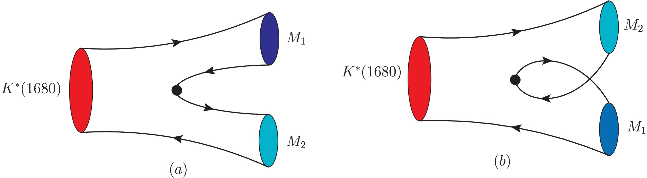
Figure 2. (color online) Illustrations of the strong decays of
$ K^*(1680) $ , treated as a$ q\bar{q} $ state, into PP or PV channels in the QPC model. The collinear mode of a hybrid decay shown in Fig. 1(a) cannot be distinguished from the QPC mechanism shown here.The QPC amplitude for a
$ q\bar{q} $ decay can be expressed in the following form:$ \begin{aligned} \begin{split} {\cal{M}}_{PP/VP}^{{\rm{QPC}}}=\gamma C^{{\rm{QPC}}}_{PP/VP}I^{{\rm{QPC}}}_{PP/VP}, \end{split} \end{aligned} $
(18) where γ is the coupling strength for creating the
$ q\bar{q} $ pair from the vacuum, and$ C_{PP/VP}^{{\rm{QPC}}} $ is a constant arising from all the Clebsch-Gordan coefficients, spin and flavor overlaps, and the energy factor$ \sqrt{E_A E_B E_C} $ ;$ I_{PP/VP}^{{\rm{QPC}}} $ is the spatial integral obtained from the convolution of the initial- and final-state wave functions and is a function of the outgoing momentum$ {\boldsymbol{p}}_B $ . In comparison with the hadron-level transition amplitudes in the ELA for Eqs. (5) and (6), the QPC amplitude can also be expressed as$\begin{aligned}[b] {\cal{M}}_{PP}^{{\rm{QPC}}}&=2g_{PP}^{{\rm{QPC}}}|{\boldsymbol{p}}_B|,\ \ \ \ PP=K^+\pi^0,K^+\eta,K^+\eta^{\prime}\\ {\cal{M}}_{VP}^{{\rm{QPC}}}&=g_{VP}^{{\rm{QPC}}}|{\boldsymbol{p}}_B|,\ \ \ \ \ VP=K^{*+}\pi^0,\rho^0K^+,\phi K^+,\omega K^+,K^{*+}\eta. \end{aligned} $
(19) By matching Eq. (18) to Eq. (19), the effective coupling constant
$ g_{PP/VP}^{{\rm{QPC}}} $ for each decay channel can be determined from the QPC amplitude.$\begin{aligned}[b]& g^{{\rm{QPC}}}_{PP}=\frac{\gamma}{2}C_{PP}^{{\rm{QPC}}}\tilde{I}_{PP}^{{\rm{QPC}}}(|{\boldsymbol{p}}_B|),\\& g^{{\rm{QPC}}}_{VP}=\gamma C_{VP}^{{\rm{QPC}}}\tilde{I}_{VP}^{{\rm{QPC}}}(|{\boldsymbol{p}}_B|), \end{aligned} $
(20) where the superscript "QPC" on
$ g_{PP} $ and$ g_{VP} $ indicates that the effective couplings are extracted from the QPC model.Consider the mixing of the conventional
$ q\bar{q} $ and hybrid components in$ K^*(1680) $ , characterized by the mixing angle ζ,$ \begin{aligned} |K^*(1680)\rangle=\cos\zeta |q\bar{q}(n^{2S+1}L_{J=1})\rangle+\sin\zeta |q\bar{q}\tilde{g}\rangle \ , \end{aligned} $
(21) where ζ is the mixing angle; n, L, S, and J are, respectively, the radial quantum number, the relative orbital angular momentum between the quark and antiquark, the total spin, and the total angular momentum of the
$ q\bar{q} $ system1 . The total amplitudes can then be expressed as$ \begin{aligned} \begin{split} {\cal{M}}_{PP/VP}^{{\rm{tot}}}&={\rm{cos}}\zeta {\cal{M}}_{PP/VP}^{{\rm{QPC}}}+{\rm{sin}}\zeta {\cal{M}}_{PP/VP}^{{\rm{FT}}}. \end{split} \end{aligned} $
(22) For
$ \zeta=0/\pi $ , the amplitudes describe the initial state$ K^*(1680) $ as a conventional$ q\bar{q} $ meson; for$ \zeta=\pi/2 $ , the amplitudes describe$ K^*(1680) $ as a pure hybrid state. The total amplitude for each decay channel is given as follows:$ \begin{aligned}[b]& {\cal{M}}_{PP}^{{\rm{tot}}}=2|{\boldsymbol{p}}_B|\left[g^{{\rm{QPC}}}_{PP}{\rm{cos}}\zeta+\left(g_{PP}^{{\rm{FT(C)}}}+g_{PP}^{{\rm{FT(T)}}}\right){\rm{sin}}\zeta\right],\\& PP=K^+\pi^0,K^+\eta,K^+\eta^{\prime},\\& {\cal{M}}_{VP}^{{\rm{tot}}}=|{\boldsymbol{p}}_B|\left[g^{{\rm{QPC}}}_{VP}{\rm{cos}}\zeta+\left(g_{VP}^{{\rm{FT(C)}}}+g_{VP}^{{\rm{FT(T)}}}\right){\rm{sin}}\zeta\right],\\& VP=K^{*+}\pi^0,\rho^0K^+,\phi K^+,\omega K^+,K^{*+}\eta. \end{aligned} $
(23) As discussed previously, the coupling strength for the collinear mode can be approximated by the QPC coupling strength, i.e.,
$ g_{PP/VP}^{{\rm{FT(C)}}}=g_{PP/VP}^{{\rm{QPC}}} $ . Thus,$ g_1^{PP/VP} $ for each decay channel can be extracted from the QPC model. At this point,$ g_1^{PP/VP} $ is a function of γ2 , the constituent quark masses$ (m_s, m_q) $ , and the harmonic oscillator parameters$ (\beta_{P}, \beta_{V}, \beta_{K^*(1680)}) $ from the wave functions. After fixing$ \alpha_P=42^\circ $ , in principle, we are left with only two free parameters, i.e., δ and ζ, in the transition amplitude. These parameters can be constrained by the experimental data, and their values can provide physical information regarding the composition of$ K^*(1680) $ .For completeness, we briefly summarize the QPC model here. In the QPC model, the process of quark-pair creation from the vacuum can be described as
$ \begin{aligned} \begin{split} \hat{T}=-3\gamma\sum_m\langle 1m;1-m|00\rangle{{(2\pi)^{3/2}}}\int {\rm d}^3{\boldsymbol{p}}_3 {\rm d}^3{\boldsymbol{p}}_4\delta^3({\boldsymbol{p}}_3+{\boldsymbol{p}}_4)y_{1m}\left(\frac{{\boldsymbol{p}}_3-{\boldsymbol{p}}_4}{2}\right)\chi_{1-m}^{34}\phi_0^{34}\omega_0^{34}b_{3i}^{\dagger}({\boldsymbol{p}}_3)d_{4j}^{\dagger}({\boldsymbol{p}}_4). \end{split} \end{aligned} $
(24) Here the momenta of the created quark and antiquark are integrated over all values, subject to the condition that their total momentum is zero; the subscripts i and j are the color SU(3) indices of the created quark and antiquark;
$ {{\boldsymbol{p}}}_i $ denotes the three-momentum of the i-th quark (antiquark);$ \phi_0^{34}=(u\bar{u}+d\bar{d}+s\bar{s})/\sqrt{3} $ ,$ \omega_0^{34}=\dfrac{1}{\sqrt{3}}\delta_{ij} $ and$ \chi_{1-m}^{34} $ are the flavor-singlet, color-singlet, and spin-triplet wave functions of the created$ q_3\bar{q}_4 $ pair, respectively; the first solid harmonic polynomial$ {\mathcal Y}_{1m}({\boldsymbol{p}})\equiv|{\boldsymbol{p}}|^1Y_{1m}(\theta,\phi) $ reflects the P-wave momentum-space distribution of the$ q_3\bar{q}_4 $ pair; γ is a dimensional constant describing the strength of quark-pair creation from the vacuum and can be extracted by fitting data. As mentioned earlier, in the collinear-mode transition of the hybrid, when the flux tube breaks, the multi-soft-gluon exchanges between the initial and final created light quark-antiquark pairs will erase the information about the initial gluelump. This makes the hybrid collinear-mode transition indistinguishable from the QPC model in two-body hadronic decays. Taking into account the multi-gluon-exchange effects, the coupling γ should be smaller than the values used in the conventional QPC model. In the center-of-mass (c.m.) frame of the initial meson$ K^*(1680) $ , the helicity amplitude can be written as$ \begin{aligned}[b] {\cal{M}}^{M_{J_A}M_{J_B}M_{J_C}} =\; &\gamma\sqrt{8E_AE_BE_C}{(2\pi)^{3/2}}\sum\langle L_AM_{L_A};S_AM_{S_A}|J_AM_{J_A}\rangle\langle L_BM_{L_B};S_BM_{S_B}|J_BM_{J_B}\rangle\\ &\times\langle L_CM_{L_C};S_CM_{S_C}|J_CM_{J_C}\rangle\langle 1m;1-m|00\rangle\langle\chi_{S_CM_{S_C}}^{32}\chi_{S_BM_{S_B}}^{14}|\chi_{S_AM_{S_A}}^{12}\chi_{1-m}^{34}\rangle\\ &\times\Bigg[\langle\phi_{C}^{32}\phi_{B}^{14}|\phi_{A}^{12}\phi_{0}^{34}\rangle I_{M_{L_B}M_{L_C}}^{M_{L_A}m}({\boldsymbol{p}}_B,m_1,m_2,m_3)\\ &+(-1)^{1+S_A+S_B+S_C}\langle\phi_{C}^{14}\phi_{B}^{32}|\phi_{A}^{12}\phi_{0}^{34}\rangle I_{M_{L_B}M_{L_C}}^{M_{L_A}m}(-{\boldsymbol{p}}_B,m_2,m_1,m_3)\Bigg], \end{aligned} $
(25) where the symbol
$ \sum $ denotes the summation over$ M_{L_A} $ ,$ M_{S_A} $ ,$ M_{L_B} $ ,$ M_{S_B} $ ,$ M_{L_C} $ ,$ M_{S_C} $ , and m. Meanwhile, the wave function convolution in momentum space has the following form:$ \begin{aligned} \begin{split} I_{M_{L_B}M_{L_C}}^{M_{L_A}m}({\boldsymbol{p}}_B,m_1,m_2,m_3)&=\int {\rm d}{\boldsymbol{p}}_3\psi_B^* \left(\frac{m_4}{m_1+m_4}{\boldsymbol{p}}_B+{\boldsymbol{p}}_3 \right)\psi_C^* \left(\frac{m_3}{m_2+m_3}{\boldsymbol{p}}_B+{\boldsymbol{p}}_3 \right) \psi_A({\boldsymbol{p}}_B+{\boldsymbol{p}}_3)y_{1m}({\boldsymbol{p}}_3). \end{split} \end{aligned} $
(26) which serves as the form factor defined at the hadronic level. The wave function in momentum space is expressed as follows:
$ \begin{aligned}[b] \psi_{nlm}({\boldsymbol{p}}, \beta) & =(-1)^n (-i)^l \sqrt{\frac{2n!} {(n + l + 1/2 )!}} \left(\frac{{\boldsymbol{p}}}{\beta}\right)^l \frac{1}{\beta^{3/2}} {\rm e}^{-\frac{{\boldsymbol{p}}^2}{2\beta^2}} L_n^{l+1/2}\left(\frac{{\boldsymbol{p}}^2}{\beta^2}\right) Y_{lm}(\theta,\phi) \equiv R_{nl}(p)Y_{lm}(\theta,\phi), \end{aligned} $
(27) where
$ L_n^a(x)=\displaystyle\sum_{k=0}^{n}(-1)^kC_{n+a}^{n-k}\frac{x^k}{k!} $ denotes the generalized Laguerre polynomial, and$ Y_{lm}(\theta,\phi) $ is the spherical harmonic function. Note that$ \psi_{nlm} $ is the wave function for the internal motion of the quarks in the harmonic oscillator (HO) basis, and β is the HO strength parameter. The wave function describing the c.m. motion is$ \delta^3({\boldsymbol{p}}-{\boldsymbol{p}}^{\prime}) $ . The corresponding normalization conditions are$ \begin{aligned}[b] &\int _0^{\infty}{\rm d} p[R_{nl}(p)]^2p^2=1,\\ &\int_0^{\pi}\int_0^{2\pi} {\rm d}\theta {\rm d}\phi Y_{l_1m_1}^*(\theta,\phi)Y_{l_2m_2}(\theta,\phi)=\delta_{l_1l_2}\delta_{m_1m_2}. \end{aligned} $
(28) Using the relativistic phase-space formalism, the decay width in the c.m. frame is given by [51]
$ \begin{aligned} \Gamma= \frac{|{\boldsymbol{p}}_B|}{8\pi M_{A}^{2}} \frac{s}{\left(2 J_{A}+1\right)} \sum_{M_{J_{A}}, M_{J_{B}}, M_{J_{C}}}\left|{\cal M}^{M_{J_{A}} M_{J_{B}} M_{J_{C}}}\right|^{2}, \end{aligned} $
(29) where
$ |{\boldsymbol{p}}_B |=\sqrt{[m_A^2-(m_B+m_C)^2][m_A^2-(m_B-m_C)^2]}/(2m_A) $ is the three-momentum of the final-state particle in the c.m. frame;$ J_A $ is the spin of the initial state; and$ s=1/(1+\delta_{BC}) $ is a statistical factor needed when B and C are identical particles. In the numerical studies, we will investigate the possibility that$ K^*(1680) $ can be assigned as either the radial excitation state$ |q\bar{q}(2^3S_1)\rangle $ or$ |q\bar{q}(3^3S_1)\rangle $ , or as the D-wave state$ |q\bar{q}(1^3D_1)\rangle $ . -
Our strategy for studying the properties of
$ K^*(1680) $ is based on the following considerations: (i) As mentioned earlier, the two-body decays of an initial$ q\bar{q} $ state can be reasonably described within the QPC model. This allows us to investigate the$ q\bar{q} $ scenario for$ K^*(1680)\to PP $ and VP as a conventional$ q\bar{q} $ state and to establish relations among these decay channels via SU(3) flavor symmetry. By assigning$ K^*(1680) $ as either the first radial excitation state$ 2^3S_1 $ or the orbital excitation state$ 1^3D_1 $ , we will examine whether it can be described within the$ q\bar{q} $ scenario. (ii) By introducing the hybrid scenario, we will also investigate the decay patterns of the initial hybrid$ K^*(1680)\to PP $ and VP, with both the collinear and transverse modes considered. (iii) We then consider$ K^*(1680) $ as a mixed state of a conventional$ q\bar{q} $ state and a hybrid. The mixing angle will be fitted through an overall description of all the two-body decay channels of$ K^*(1680)\to PP $ and VP.At the hadronic level, the decay of an initial vector meson into PP and VP can be described by effective Lagrangians. With V and P denoting the ground-state vector and pseudoscalar mesons, respectively, SU(3) flavor symmetry allows us to establish connections among all the PP and VP decay channels. The following effective Lagrangians are adopted:
$ \begin{aligned} {\cal{L}}_{VPP}&= {\rm i} g_{VPP} {\rm Tr} [(P\partial_{\mu}P- \partial_{\mu}P P)V^{\mu}], \end{aligned} $
(1) $ \begin{aligned} {\cal{L}}_{VVP}&= \frac{1}{m_V} g_{VVP}\epsilon_{\alpha\beta\mu\nu} {\rm Tr} [\partial^\alpha V^\mu \partial^\beta V^\nu P], \end{aligned} $
(2) where
$ g_{VPP} $ and$ g_{VVP} $ are dimensionless coupling strengths. Here, V and P denote the vector and pseudoscalar fields of the ground-state SU(3) nonet, respectively, and take the following forms$ \begin{aligned} P & = \left( \begin{array}{*{20}{c}} {\dfrac{{\sin {\alpha _P}\eta' + \cos {\alpha _P}\eta + {\pi ^0}}}{{\sqrt 2 }}}&{{\pi ^ + }}&{{K^ + }}\\ \pi^- &{\dfrac{{\sin {\alpha _P}\eta' + \cos {\alpha _P}\eta - {\pi ^0}}}{{\sqrt 2 }}}&{{K^0}}\\ {{K^ - }}&{{{\bar K}^0}}&{\cos {\alpha_P}\eta' - \sin {\alpha _P}\eta } \end{array} \right), \end{aligned} $
(3) and
$ \begin{aligned} V &= \left( \begin{array}{*{20}{c}} \dfrac{\omega + \rho ^0}{\sqrt 2}&\rho^+&K^{*+}\\ \rho^-&\dfrac{\omega - \rho ^0}{\sqrt 2}&K^{*0}\\ {{K^{* - }}}&{{{\bar K}^{*0}}}&\phi \end{array} \right). \end{aligned} $
(4) In the vector sector, ideal mixing between
$ \omega=(u\bar u + d\bar d)/ \sqrt 2 $ and$ \phi = s\bar s $ is adopted. As for η and$ \eta' $ , they can be expressed in the quark-flavor basis as$ \eta = \cos \alpha_P n\bar n - \sin\alpha_P s\bar s $ and$ \eta' = \sin \alpha_P n\bar n + \cos\alpha_P s\bar s $ , where$ n\bar n \equiv (u\bar u + d\bar d)/\sqrt2 $ , and the mixing angle$ \alpha_P \equiv \arctan\sqrt 2 + \theta_p $ , with$ \theta_p $ being the flavor singlet-octet mixing angle. For the two-body hadronic decays, most of the$ K^*(1680) \to PP $ and VP decay channels are kinematically allowed. We focus on the PP and VP decay channels, taking into account the experimental situation. The hadronic-level transition amplitudes in the effective Lagrangian approach (ELA) are as follows:$ \begin{aligned} {\rm i}{\cal{M}}_{VPP}^{{\rm{ELA}}}&= {\rm i} g_{VPP}(p_B-p_C)_{\mu}\epsilon_A^{\mu} = {\rm i} g_{VPP} 2 |{\boldsymbol{p}}_B|, \end{aligned} $
(5) $ \begin{aligned} {\rm i}{\cal{M}}_{VVP}^{{\rm{ELA}}}&= \frac{1}{m_A} {\rm i} g_{VVP}\epsilon_{\alpha\beta\mu\nu} p_A^{\alpha}p_B^{\beta}\epsilon_A^{\mu}{\epsilon_B^{\nu}}^* = {\rm i} g_{VVP}m_A |{\boldsymbol{p}}_B|. \end{aligned} $
(6) The coupling constants defined above can receive contributions from the decay of the conventional
$ q\bar{q} $ component via the QPC model and from the decay of the hybrid component via the FT model.As discussed earlier, the FT model actually contains the QPC model. Its collinear mode shares dynamics similar to those of the QPC model in the decay. Since we consider only the decays of a fixed set of processes, namely
$ K^*(1680)\to VP $ and PP, we assume that the collinear mode can be described by the QPC model. Meanwhile, the transverse mode is driven by a different mechanism. These are two independent mechanisms for hybrid decays and are illustrated in Fig. 1 (a) and (b), respectively. At the quark level, Fig. 1 (a) dominates the collinear mode and describes the breaking of the flux-tube string through the creation of a$ q\bar{q} $ pair that combines with the initial quark and antiquark. With multi-gluon exchanges during hadronization, Fig. 1 (a) behaves similarly to the QPC transition. This allows us to evaluate the coupling of the collinear-mode decay using the QPC model and to unify these two mechanisms within the same framework.
Figure 1. (color online) Schematic illustrations of the two-body hadronic decays of hybrid states. Panel (a) is dominated by the collinear mode, while panel (b) is dominated by the transverse mode.
The hybrid decay via the transverse mode dominates the process shown in Fig. 1 (b). The quark pair created by the transverse mode causes the initial quark-antiquark pair to recoil through the transverse flux motion. Then, with a soft gluon exchange that neutralizes the color of the recoiled
$ q\bar{q} $ pair, the process shown in Fig. 1 (b) plays a crucial and unique role in decay channels involving the production of flavor-singlet hadrons. For conventional$ q\bar{q} $ decays, a process similar to that shown in Fig. 1 (b) may also occur. However, it is usually suppressed by the Okubo-Zweig-Iizuka (OZI) rule. In contrast, in the decay of a hybrid, Fig. 1 (b) is not necessarily suppressed [50].With the above considerations, we can define the transition amplitude for a
$ 1^{-+} $ hybrid of$ q\bar{q}\tilde{g} $ decaying into two conventional mesons, PP and VP, as follows [4]$ \begin{aligned}[b] &{\cal{M}}_a^{VPP}= \langle(q_1\bar{q_4})_{P} (q_3\bar{q_2})_{P}|\hat V_C|q_1\bar{q_2}\tilde{g}\rangle \equiv g_{1}^{VPP}|{\boldsymbol{p}}_B |, \\ &{\cal{M}}_b^{VPP}= \langle(q_1\bar{q_2})_{P} (q_3\bar{q_4})_{P}|\hat V_T|q_1\bar{q_2}\tilde{g}\rangle \equiv g_{2}^{VPP}|{\boldsymbol{p}}_B |, \\ &{\cal{M}}_a^{VVP}= \langle(q_1\bar{q_4})_{P(V)} (q_3\bar{q_2})_{V(P)}|\hat V_C|q_1\bar{q_2}\tilde{g}\rangle \equiv g_{1}^{VVP}|{\boldsymbol{p}}_B |, \\ &{\cal{M}}_b^{VVP}= \langle(q_1\bar{q_2})_{P(V)} (q_3\bar{q_4})_{V(P)}|\hat V_T|q_1\bar{q_2}\tilde{g}\rangle \equiv g_{2}^{VVP}|{\boldsymbol{p}}_B |, \end{aligned} $
(7) where
$ {\cal{M}}_a $ and$ {\cal{M}}_b $ are the amplitudes corresponding to the collinear and transverse flux excitations, respectively, and$ \hat{V}_C $ and$ \hat{V}_T $ are the corresponding interaction potentials.$ |{\boldsymbol{p}}_B | $ is the three-momentum of the final-state meson in the c.m. frame of the initial hybrid.By matching the transition amplitudes defined at the quark level to those defined at the hadronic level, we obtain the following relations for the hybrid-state decays
$ K^*(1680)\to PP $ and VP:$ \begin{aligned}[b] {\cal{M}}^{{\rm{FT}}}_{PP}&=2g_{PP}^{{\rm{FT}}}|{\boldsymbol{p}}_B|,\ \ \ \ PP=K^+\pi^0,K^+\eta,K^+\eta^{\prime},\\ {\cal{M}}^{{\rm{FT}}}_{VP}&=g_{VP}^{{\rm{FT}}}|{\boldsymbol{p}}_B|,\ \ \ \ \ VP=K^{*+}\pi^0,\rho^0K^+,\phi K^+,\omega K^+,K^{*+}\eta \ . \end{aligned} $
(8) The above relations allow a unified description of the decay processes in terms of the two coupling constants
$ g_1 $ and$ g_2 $ , with which the hadronic couplings$ g_{PP/VP}^{{\rm{FT}}} $ for the eight decay channels$ K^{*+}(1680)\to PP $ and VP can be parameterized as$ \begin{aligned} g_{PP/VP}^{{\rm{FT}}}=g_{PP/VP}^{{\rm{FT(C)}}}(g_1)+g_{PP/VP}^{{\rm{FT(T)}}}(g_2) \ . \end{aligned} $
(9) The specific expression for each channel can be obtained as follows:
$ \begin{aligned} g_{K^+\pi^0}^{{\rm{FT(C)}}}&=\frac{1}{\sqrt{2}}g_1^{K^+\pi^0},&g_{K^+\pi^0}^{{\rm{FT(T)}}}&=0, \end{aligned} $
(10) $ \begin{aligned}[b]& g_{K^+\eta}^{{\rm{FT(C)}}}&=\left(\frac{1}{\sqrt{2}}{\rm{cos}}\alpha_P-R{\rm{sin}}\alpha_P\right)g_{1}^{K^+\eta},\\& g_{K^+\eta}^{{\rm{FT(T)}}}&=\left(\sqrt{2}{\rm{cos}}\alpha_P-R{\rm{sin}}\alpha_P\right)\delta g_{1}^{K^+\eta}, \end{aligned} $
(11) $ \begin{aligned}[b]& g_{K^+\eta^{\prime}}^{{\rm{FT(C)}}}&=\left(\frac{1}{\sqrt{2}}{\rm{sin}}\alpha_P+R{\rm{cos}}\alpha_P\right)g_{1}^{K^+\eta^{\prime}},\\&g_{K^+\eta^{\prime}}^{{\rm{FT(T)}}}&=\left(\sqrt{2}{\rm{sin}}\alpha_P+R{\rm{cos}}\alpha_P\right)\delta g_{1}^{K^+\eta^{\prime}}, \end{aligned} $
(12) $ \begin{aligned} g_{K^{*+}\pi^0}^{{\rm{FT(C)}}}&=\frac{1}{\sqrt{2}}g_1^{K^{*+}\pi^0},&g_{K^{*+}\pi^0}^{{\rm{FT(T)}}}&=0 \end{aligned} $
(13) $ \begin{aligned} g_{K^+\rho^0}^{{\rm{FT(C)}}}&=\frac{1}{\sqrt{2}}g_1^{K^+\rho^0},&g_{K^+\rho^0}^{{\rm{FT(T)}}}&=0, \end{aligned} $
(14) $ \begin{aligned} g_{K^+\omega}^{{\rm{FT(C)}}}&=\frac{1}{\sqrt{2}}g_1^{K^+\omega},&g_{K^+\omega}^{{\rm{FT(T)}}}&=\frac{2}{\sqrt{2}}\delta g_1^{K^+\omega}, \end{aligned} $
(15) $ \begin{aligned} g_{K^+\phi}^{{\rm{FT(C)}}}&=Rg_1^{K^+\phi},&g_{K^+\phi}^{{\rm{FT(T)}}}&=R\delta g_1^{K^+\phi}, \end{aligned} $
(16) $ \begin{aligned}[b]& g_{K^{*+}\eta}^{{\rm{FT(C)}}}=\left(\frac{1}{\sqrt{2}}{\rm{cos}}\alpha_P-R{\rm{sin}}\alpha_P\right)g_{1}^{K^{*+}\eta},\\&g_{K^{*+}\eta}^{{\rm{FT(T)}}}=\left(\sqrt{2}{\rm{cos}}\alpha_P-R{\rm{sin}}\alpha_P\right)\delta g_{1}^{K^{*+}\eta}, \end{aligned} $
(17) where we label the decay channels in the superscripts of
$ g_1 $ and$ g_2 $ to highlight the possible differences arising from their distinct spatial convolutions in different decay channels. The ratio$ \delta \equiv g_2/g_1 $ stands for the relative strength of the two couplings$ g_{1,2} $ . For decay channels in which the final states contain no isoscalar mesons,$ g_2 $ should vanish. For instance, in$ K^*(1680)\to K\pi $ , only Fig. 1 (a) contributes. In this sense, it is difficult to distinguish between the$ q\bar{q} $ and$ q\bar{q}\tilde{g} $ scenarios.The assumption that the collinear mode can be described by the QPC model makes it possible to quantify this amplitude through explicit calculations.
To proceed, we employ the QPC model to extract the transition amplitudes for the
$ q\bar{q} $ scenario (see Fig. 2). These amplitudes can provide an estimate of the collinear-mode amplitudes for the hybrid scenario. Then, by introducing the relative coupling strength δ, one can evaluate all the decay channels of$ K^*(1680)\to PP $ and VP.
Figure 2. (color online) Illustrations of the strong decays of
$ K^*(1680) $ , treated as a$ q\bar{q} $ state, into PP or PV channels in the QPC model. The collinear mode of a hybrid decay shown in Fig. 1(a) cannot be distinguished from the QPC mechanism shown here.The QPC amplitude for a
$ q\bar{q} $ decay can be expressed in the following form:$ \begin{aligned} \begin{split} {\cal{M}}_{PP/VP}^{{\rm{QPC}}}=\gamma C^{{\rm{QPC}}}_{PP/VP}I^{{\rm{QPC}}}_{PP/VP}, \end{split} \end{aligned} $
(18) where γ is the coupling strength for creating the
$ q\bar{q} $ pair from the vacuum, and$ C_{PP/VP}^{{\rm{QPC}}} $ is a constant arising from all the Clebsch-Gordan coefficients, spin and flavor overlaps, and the energy factor$ \sqrt{E_A E_B E_C} $ ;$ I_{PP/VP}^{{\rm{QPC}}} $ is the spatial integral obtained from the convolution of the initial- and final-state wave functions and is a function of the outgoing momentum$ {\boldsymbol{p}}_B $ . In comparison with the hadron-level transition amplitudes in the ELA for Eqs. (5) and (6), the QPC amplitude can also be expressed as$\begin{aligned}[b] {\cal{M}}_{PP}^{{\rm{QPC}}}&=2g_{PP}^{{\rm{QPC}}}|{\boldsymbol{p}}_B|,\ \ \ \ PP=K^+\pi^0,K^+\eta,K^+\eta^{\prime}\\ {\cal{M}}_{VP}^{{\rm{QPC}}}&=g_{VP}^{{\rm{QPC}}}|{\boldsymbol{p}}_B|,\ \ \ \ \ VP=K^{*+}\pi^0,\rho^0K^+,\phi K^+,\omega K^+,K^{*+}\eta. \end{aligned} $
(19) By matching Eq. (18) to Eq. (19), the effective coupling constant
$ g_{PP/VP}^{{\rm{QPC}}} $ for each decay channel can be determined from the QPC amplitude.$\begin{aligned}[b]& g^{{\rm{QPC}}}_{PP}=\frac{\gamma}{2}C_{PP}^{{\rm{QPC}}}\tilde{I}_{PP}^{{\rm{QPC}}}(|{\boldsymbol{p}}_B|),\\& g^{{\rm{QPC}}}_{VP}=\gamma C_{VP}^{{\rm{QPC}}}\tilde{I}_{VP}^{{\rm{QPC}}}(|{\boldsymbol{p}}_B|), \end{aligned} $
(20) where the superscript "QPC" on
$ g_{PP} $ and$ g_{VP} $ indicates that the effective couplings are extracted from the QPC model.Consider the mixing of the conventional
$ q\bar{q} $ and hybrid components in$ K^*(1680) $ , characterized by the mixing angle ζ,$ \begin{aligned} |K^*(1680)\rangle=\cos\zeta |q\bar{q}(n^{2S+1}L_{J=1})\rangle+\sin\zeta |q\bar{q}\tilde{g}\rangle \ , \end{aligned} $
(21) where ζ is the mixing angle; n, L, S, and J are, respectively, the radial quantum number, the relative orbital angular momentum between the quark and antiquark, the total spin, and the total angular momentum of the
$ q\bar{q} $ system1 . The total amplitudes can then be expressed as$ \begin{aligned} \begin{split} {\cal{M}}_{PP/VP}^{{\rm{tot}}}&={\rm{cos}}\zeta {\cal{M}}_{PP/VP}^{{\rm{QPC}}}+{\rm{sin}}\zeta {\cal{M}}_{PP/VP}^{{\rm{FT}}}. \end{split} \end{aligned} $
(22) For
$ \zeta=0/\pi $ , the amplitudes describe the initial state$ K^*(1680) $ as a conventional$ q\bar{q} $ meson; for$ \zeta=\pi/2 $ , the amplitudes describe$ K^*(1680) $ as a pure hybrid state. The total amplitude for each decay channel is given as follows:$ \begin{aligned}[b]& {\cal{M}}_{PP}^{{\rm{tot}}}=2|{\boldsymbol{p}}_B|\left[g^{{\rm{QPC}}}_{PP}{\rm{cos}}\zeta+\left(g_{PP}^{{\rm{FT(C)}}}+g_{PP}^{{\rm{FT(T)}}}\right){\rm{sin}}\zeta\right],\\& PP=K^+\pi^0,K^+\eta,K^+\eta^{\prime},\\& {\cal{M}}_{VP}^{{\rm{tot}}}=|{\boldsymbol{p}}_B|\left[g^{{\rm{QPC}}}_{VP}{\rm{cos}}\zeta+\left(g_{VP}^{{\rm{FT(C)}}}+g_{VP}^{{\rm{FT(T)}}}\right){\rm{sin}}\zeta\right],\\& VP=K^{*+}\pi^0,\rho^0K^+,\phi K^+,\omega K^+,K^{*+}\eta. \end{aligned} $
(23) As discussed previously, the coupling strength for the collinear mode can be approximated by the QPC coupling strength, i.e.,
$ g_{PP/VP}^{{\rm{FT(C)}}}=g_{PP/VP}^{{\rm{QPC}}} $ . Thus,$ g_1^{PP/VP} $ for each decay channel can be extracted from the QPC model. At this point,$ g_1^{PP/VP} $ is a function of γ2 , the constituent quark masses$ (m_s, m_q) $ , and the harmonic oscillator parameters$ (\beta_{P}, \beta_{V}, \beta_{K^*(1680)}) $ from the wave functions. After fixing$ \alpha_P=42^\circ $ , in principle, we are left with only two free parameters, i.e., δ and ζ, in the transition amplitude. These parameters can be constrained by the experimental data, and their values can provide physical information regarding the composition of$ K^*(1680) $ .For completeness, we briefly summarize the QPC model here. In the QPC model, the process of quark-pair creation from the vacuum can be described as
$ \begin{aligned} \begin{split} \hat{T}=-3\gamma\sum_m\langle 1m;1-m|00\rangle{{(2\pi)^{3/2}}}\int {\rm d}^3{\boldsymbol{p}}_3 {\rm d}^3{\boldsymbol{p}}_4\delta^3({\boldsymbol{p}}_3+{\boldsymbol{p}}_4)y_{1m}\left(\frac{{\boldsymbol{p}}_3-{\boldsymbol{p}}_4}{2}\right)\chi_{1-m}^{34}\phi_0^{34}\omega_0^{34}b_{3i}^{\dagger}({\boldsymbol{p}}_3)d_{4j}^{\dagger}({\boldsymbol{p}}_4). \end{split} \end{aligned} $
(24) Here the momenta of the created quark and antiquark are integrated over all values, subject to the condition that their total momentum is zero; the subscripts i and j are the color SU(3) indices of the created quark and antiquark;
$ {{\boldsymbol{p}}}_i $ denotes the three-momentum of the i-th quark (antiquark);$ \phi_0^{34}=(u\bar{u}+d\bar{d}+s\bar{s})/\sqrt{3} $ ,$ \omega_0^{34}=\dfrac{1}{\sqrt{3}}\delta_{ij} $ and$ \chi_{1-m}^{34} $ are the flavor-singlet, color-singlet, and spin-triplet wave functions of the created$ q_3\bar{q}_4 $ pair, respectively; the first solid harmonic polynomial$ {\mathcal Y}_{1m}({\boldsymbol{p}})\equiv|{\boldsymbol{p}}|^1Y_{1m}(\theta,\phi) $ reflects the P-wave momentum-space distribution of the$ q_3\bar{q}_4 $ pair; γ is a dimensional constant describing the strength of quark-pair creation from the vacuum and can be extracted by fitting data. As mentioned earlier, in the collinear-mode transition of the hybrid, when the flux tube breaks, the multi-soft-gluon exchanges between the initial and final created light quark-antiquark pairs will erase the information about the initial gluelump. This makes the hybrid collinear-mode transition indistinguishable from the QPC model in two-body hadronic decays. Taking into account the multi-gluon-exchange effects, the coupling γ should be smaller than the values used in the conventional QPC model. In the center-of-mass (c.m.) frame of the initial meson$ K^*(1680) $ , the helicity amplitude can be written as$ \begin{aligned}[b] {\cal{M}}^{M_{J_A}M_{J_B}M_{J_C}} =\; &\gamma\sqrt{8E_AE_BE_C}{(2\pi)^{3/2}}\sum\langle L_AM_{L_A};S_AM_{S_A}|J_AM_{J_A}\rangle\langle L_BM_{L_B};S_BM_{S_B}|J_BM_{J_B}\rangle\\ &\times\langle L_CM_{L_C};S_CM_{S_C}|J_CM_{J_C}\rangle\langle 1m;1-m|00\rangle\langle\chi_{S_CM_{S_C}}^{32}\chi_{S_BM_{S_B}}^{14}|\chi_{S_AM_{S_A}}^{12}\chi_{1-m}^{34}\rangle\\ &\times\Bigg[\langle\phi_{C}^{32}\phi_{B}^{14}|\phi_{A}^{12}\phi_{0}^{34}\rangle I_{M_{L_B}M_{L_C}}^{M_{L_A}m}({\boldsymbol{p}}_B,m_1,m_2,m_3)\\ &+(-1)^{1+S_A+S_B+S_C}\langle\phi_{C}^{14}\phi_{B}^{32}|\phi_{A}^{12}\phi_{0}^{34}\rangle I_{M_{L_B}M_{L_C}}^{M_{L_A}m}(-{\boldsymbol{p}}_B,m_2,m_1,m_3)\Bigg], \end{aligned} $
(25) where the symbol
$ \sum $ denotes the summation over$ M_{L_A} $ ,$ M_{S_A} $ ,$ M_{L_B} $ ,$ M_{S_B} $ ,$ M_{L_C} $ ,$ M_{S_C} $ , and m. Meanwhile, the wave function convolution in momentum space has the following form:$ \begin{aligned} \begin{split} I_{M_{L_B}M_{L_C}}^{M_{L_A}m}({\boldsymbol{p}}_B,m_1,m_2,m_3)&=\int {\rm d}{\boldsymbol{p}}_3\psi_B^* \left(\frac{m_4}{m_1+m_4}{\boldsymbol{p}}_B+{\boldsymbol{p}}_3 \right)\psi_C^* \left(\frac{m_3}{m_2+m_3}{\boldsymbol{p}}_B+{\boldsymbol{p}}_3 \right) \psi_A({\boldsymbol{p}}_B+{\boldsymbol{p}}_3)y_{1m}({\boldsymbol{p}}_3). \end{split} \end{aligned} $
(26) which serves as the form factor defined at the hadronic level. The wave function in momentum space is expressed as follows:
$ \begin{aligned}[b] \psi_{nlm}({\boldsymbol{p}}, \beta) & =(-1)^n (-i)^l \sqrt{\frac{2n!} {(n + l + 1/2 )!}} \left(\frac{{\boldsymbol{p}}}{\beta}\right)^l \frac{1}{\beta^{3/2}} {\rm e}^{-\frac{{\boldsymbol{p}}^2}{2\beta^2}} L_n^{l+1/2}\left(\frac{{\boldsymbol{p}}^2}{\beta^2}\right) Y_{lm}(\theta,\phi) \equiv R_{nl}(p)Y_{lm}(\theta,\phi), \end{aligned} $
(27) where
$ L_n^a(x)=\displaystyle\sum_{k=0}^{n}(-1)^kC_{n+a}^{n-k}\frac{x^k}{k!} $ denotes the generalized Laguerre polynomial, and$ Y_{lm}(\theta,\phi) $ is the spherical harmonic function. Note that$ \psi_{nlm} $ is the wave function for the internal motion of the quarks in the harmonic oscillator (HO) basis, and β is the HO strength parameter. The wave function describing the c.m. motion is$ \delta^3({\boldsymbol{p}}-{\boldsymbol{p}}^{\prime}) $ . The corresponding normalization conditions are$ \begin{aligned}[b] &\int _0^{\infty}{\rm d} p[R_{nl}(p)]^2p^2=1,\\ &\int_0^{\pi}\int_0^{2\pi} {\rm d}\theta {\rm d}\phi Y_{l_1m_1}^*(\theta,\phi)Y_{l_2m_2}(\theta,\phi)=\delta_{l_1l_2}\delta_{m_1m_2}. \end{aligned} $
(28) Using the relativistic phase-space formalism, the decay width in the c.m. frame is given by [51]
$ \begin{aligned} \Gamma= \frac{|{\boldsymbol{p}}_B|}{8\pi M_{A}^{2}} \frac{s}{\left(2 J_{A}+1\right)} \sum_{M_{J_{A}}, M_{J_{B}}, M_{J_{C}}}\left|{\cal M}^{M_{J_{A}} M_{J_{B}} M_{J_{C}}}\right|^{2}, \end{aligned} $
(29) where
$ |{\boldsymbol{p}}_B |=\sqrt{[m_A^2-(m_B+m_C)^2][m_A^2-(m_B-m_C)^2]}/(2m_A) $ is the three-momentum of the final-state particle in the c.m. frame;$ J_A $ is the spin of the initial state; and$ s=1/(1+\delta_{BC}) $ is a statistical factor needed when B and C are identical particles. In the numerical studies, we will investigate the possibility that$ K^*(1680) $ can be assigned as either the radial excitation state$ |q\bar{q}(2^3S_1)\rangle $ or$ |q\bar{q}(3^3S_1)\rangle $ , or as the D-wave state$ |q\bar{q}(1^3D_1)\rangle $ . -
Our strategy for studying the properties of
$ K^*(1680) $ is based on the following considerations: (i) As mentioned earlier, the two-body decays of an initial$ q\bar{q} $ state can be reasonably described within the QPC model. This allows us to investigate the$ q\bar{q} $ scenario for$ K^*(1680)\to PP $ and VP as a conventional$ q\bar{q} $ state and to establish relations among these decay channels via SU(3) flavor symmetry. By assigning$ K^*(1680) $ as either the first radial excitation state$ 2^3S_1 $ or the orbital excitation state$ 1^3D_1 $ , we will examine whether it can be described within the$ q\bar{q} $ scenario. (ii) By introducing the hybrid scenario, we will also investigate the decay patterns of the initial hybrid$ K^*(1680)\to PP $ and VP, with both the collinear and transverse modes considered. (iii) We then consider$ K^*(1680) $ as a mixed state of a conventional$ q\bar{q} $ state and a hybrid. The mixing angle will be fitted through an overall description of all the two-body decay channels of$ K^*(1680)\to PP $ and VP.At the hadronic level, the decay of an initial vector meson into PP and VP can be described by effective Lagrangians. With V and P denoting the ground-state vector and pseudoscalar mesons, respectively, SU(3) flavor symmetry allows us to establish connections among all the PP and VP decay channels. The following effective Lagrangians are adopted:
$ \begin{aligned} {\cal{L}}_{VPP}&= {\rm i} g_{VPP} {\rm Tr} [(P\partial_{\mu}P- \partial_{\mu}P P)V^{\mu}], \end{aligned} $
(1) $ \begin{aligned} {\cal{L}}_{VVP}&= \frac{1}{m_V} g_{VVP}\epsilon_{\alpha\beta\mu\nu} {\rm Tr} [\partial^\alpha V^\mu \partial^\beta V^\nu P], \end{aligned} $
(2) where
$ g_{VPP} $ and$ g_{VVP} $ are dimensionless coupling strengths. Here, V and P denote the vector and pseudoscalar fields of the ground-state SU(3) nonet, respectively, and take the following forms$ \begin{aligned} P & = \left( \begin{array}{*{20}{c}} {\dfrac{{\sin {\alpha _P}\eta' + \cos {\alpha _P}\eta + {\pi ^0}}}{{\sqrt 2 }}}&{{\pi ^ + }}&{{K^ + }}\\ \pi^- &{\dfrac{{\sin {\alpha _P}\eta' + \cos {\alpha _P}\eta - {\pi ^0}}}{{\sqrt 2 }}}&{{K^0}}\\ {{K^ - }}&{{{\bar K}^0}}&{\cos {\alpha_P}\eta' - \sin {\alpha _P}\eta } \end{array} \right), \end{aligned} $
(3) and
$ \begin{aligned} V &= \left( \begin{array}{*{20}{c}} \dfrac{\omega + \rho ^0}{\sqrt 2}&\rho^+&K^{*+}\\ \rho^-&\dfrac{\omega - \rho ^0}{\sqrt 2}&K^{*0}\\ {{K^{* - }}}&{{{\bar K}^{*0}}}&\phi \end{array} \right). \end{aligned} $
(4) In the vector sector, ideal mixing between
$ \omega=(u\bar u + d\bar d)/ \sqrt 2 $ and$ \phi = s\bar s $ is adopted. As for η and$ \eta' $ , they can be expressed in the quark-flavor basis as$ \eta = \cos \alpha_P n\bar n - \sin\alpha_P s\bar s $ and$ \eta' = \sin \alpha_P n\bar n + \cos\alpha_P s\bar s $ , where$ n\bar n \equiv (u\bar u + d\bar d)/\sqrt2 $ , and the mixing angle$ \alpha_P \equiv \arctan\sqrt 2 + \theta_p $ , with$ \theta_p $ being the flavor singlet-octet mixing angle. For the two-body hadronic decays, most of the$ K^*(1680) \to PP $ and VP decay channels are kinematically allowed. We focus on the PP and VP decay channels, taking into account the experimental situation. The hadronic-level transition amplitudes in the effective Lagrangian approach (ELA) are as follows:$ \begin{aligned} {\rm i}{\cal{M}}_{VPP}^{{\rm{ELA}}}&= {\rm i} g_{VPP}(p_B-p_C)_{\mu}\epsilon_A^{\mu} = {\rm i} g_{VPP} 2 |{\boldsymbol{p}}_B|, \end{aligned} $
(5) $ \begin{aligned} {\rm i}{\cal{M}}_{VVP}^{{\rm{ELA}}}&= \frac{1}{m_A} {\rm i} g_{VVP}\epsilon_{\alpha\beta\mu\nu} p_A^{\alpha}p_B^{\beta}\epsilon_A^{\mu}{\epsilon_B^{\nu}}^* = {\rm i} g_{VVP}m_A |{\boldsymbol{p}}_B|. \end{aligned} $
(6) The coupling constants defined above can receive contributions from the decay of the conventional
$ q\bar{q} $ component via the QPC model and from the decay of the hybrid component via the FT model.As discussed earlier, the FT model actually contains the QPC model. Its collinear mode shares dynamics similar to those of the QPC model in the decay. Since we consider only the decays of a fixed set of processes, namely
$ K^*(1680)\to VP $ and PP, we assume that the collinear mode can be described by the QPC model. Meanwhile, the transverse mode is driven by a different mechanism. These are two independent mechanisms for hybrid decays and are illustrated in Fig. 1 (a) and (b), respectively. At the quark level, Fig. 1 (a) dominates the collinear mode and describes the breaking of the flux-tube string through the creation of a$ q\bar{q} $ pair that combines with the initial quark and antiquark. With multi-gluon exchanges during hadronization, Fig. 1 (a) behaves similarly to the QPC transition. This allows us to evaluate the coupling of the collinear-mode decay using the QPC model and to unify these two mechanisms within the same framework.
Figure 1. (color online) Schematic illustrations of the two-body hadronic decays of hybrid states. Panel (a) is dominated by the collinear mode, while panel (b) is dominated by the transverse mode.
The hybrid decay via the transverse mode dominates the process shown in Fig. 1 (b). The quark pair created by the transverse mode causes the initial quark-antiquark pair to recoil through the transverse flux motion. Then, with a soft gluon exchange that neutralizes the color of the recoiled
$ q\bar{q} $ pair, the process shown in Fig. 1 (b) plays a crucial and unique role in decay channels involving the production of flavor-singlet hadrons. For conventional$ q\bar{q} $ decays, a process similar to that shown in Fig. 1 (b) may also occur. However, it is usually suppressed by the Okubo-Zweig-Iizuka (OZI) rule. In contrast, in the decay of a hybrid, Fig. 1 (b) is not necessarily suppressed [50].With the above considerations, we can define the transition amplitude for a
$ 1^{-+} $ hybrid of$ q\bar{q}\tilde{g} $ decaying into two conventional mesons, PP and VP, as follows [4]$ \begin{aligned}[b] &{\cal{M}}_a^{VPP}= \langle(q_1\bar{q_4})_{P} (q_3\bar{q_2})_{P}|\hat V_C|q_1\bar{q_2}\tilde{g}\rangle \equiv g_{1}^{VPP}|{\boldsymbol{p}}_B |, \\ &{\cal{M}}_b^{VPP}= \langle(q_1\bar{q_2})_{P} (q_3\bar{q_4})_{P}|\hat V_T|q_1\bar{q_2}\tilde{g}\rangle \equiv g_{2}^{VPP}|{\boldsymbol{p}}_B |, \\ &{\cal{M}}_a^{VVP}= \langle(q_1\bar{q_4})_{P(V)} (q_3\bar{q_2})_{V(P)}|\hat V_C|q_1\bar{q_2}\tilde{g}\rangle \equiv g_{1}^{VVP}|{\boldsymbol{p}}_B |, \\ &{\cal{M}}_b^{VVP}= \langle(q_1\bar{q_2})_{P(V)} (q_3\bar{q_4})_{V(P)}|\hat V_T|q_1\bar{q_2}\tilde{g}\rangle \equiv g_{2}^{VVP}|{\boldsymbol{p}}_B |, \end{aligned} $
(7) where
$ {\cal{M}}_a $ and$ {\cal{M}}_b $ are the amplitudes corresponding to the collinear and transverse flux excitations, respectively, and$ \hat{V}_C $ and$ \hat{V}_T $ are the corresponding interaction potentials.$ |{\boldsymbol{p}}_B | $ is the three-momentum of the final-state meson in the c.m. frame of the initial hybrid.By matching the transition amplitudes defined at the quark level to those defined at the hadronic level, we obtain the following relations for the hybrid-state decays
$ K^*(1680)\to PP $ and VP:$ \begin{aligned}[b] {\cal{M}}^{{\rm{FT}}}_{PP}&=2g_{PP}^{{\rm{FT}}}|{\boldsymbol{p}}_B|,\ \ \ \ PP=K^+\pi^0,K^+\eta,K^+\eta^{\prime},\\ {\cal{M}}^{{\rm{FT}}}_{VP}&=g_{VP}^{{\rm{FT}}}|{\boldsymbol{p}}_B|,\ \ \ \ \ VP=K^{*+}\pi^0,\rho^0K^+,\phi K^+,\omega K^+,K^{*+}\eta \ . \end{aligned} $
(8) The above relations allow a unified description of the decay processes in terms of the two coupling constants
$ g_1 $ and$ g_2 $ , with which the hadronic couplings$ g_{PP/VP}^{{\rm{FT}}} $ for the eight decay channels$ K^{*+}(1680)\to PP $ and VP can be parameterized as$ \begin{aligned} g_{PP/VP}^{{\rm{FT}}}=g_{PP/VP}^{{\rm{FT(C)}}}(g_1)+g_{PP/VP}^{{\rm{FT(T)}}}(g_2) \ . \end{aligned} $
(9) The specific expression for each channel can be obtained as follows:
$ \begin{aligned} g_{K^+\pi^0}^{{\rm{FT(C)}}}&=\frac{1}{\sqrt{2}}g_1^{K^+\pi^0},&g_{K^+\pi^0}^{{\rm{FT(T)}}}&=0, \end{aligned} $
(10) $ \begin{aligned}[b]& g_{K^+\eta}^{{\rm{FT(C)}}}&=\left(\frac{1}{\sqrt{2}}{\rm{cos}}\alpha_P-R{\rm{sin}}\alpha_P\right)g_{1}^{K^+\eta},\\& g_{K^+\eta}^{{\rm{FT(T)}}}&=\left(\sqrt{2}{\rm{cos}}\alpha_P-R{\rm{sin}}\alpha_P\right)\delta g_{1}^{K^+\eta}, \end{aligned} $
(11) $ \begin{aligned}[b]& g_{K^+\eta^{\prime}}^{{\rm{FT(C)}}}&=\left(\frac{1}{\sqrt{2}}{\rm{sin}}\alpha_P+R{\rm{cos}}\alpha_P\right)g_{1}^{K^+\eta^{\prime}},\\&g_{K^+\eta^{\prime}}^{{\rm{FT(T)}}}&=\left(\sqrt{2}{\rm{sin}}\alpha_P+R{\rm{cos}}\alpha_P\right)\delta g_{1}^{K^+\eta^{\prime}}, \end{aligned} $
(12) $ \begin{aligned} g_{K^{*+}\pi^0}^{{\rm{FT(C)}}}&=\frac{1}{\sqrt{2}}g_1^{K^{*+}\pi^0},&g_{K^{*+}\pi^0}^{{\rm{FT(T)}}}&=0 \end{aligned} $
(13) $ \begin{aligned} g_{K^+\rho^0}^{{\rm{FT(C)}}}&=\frac{1}{\sqrt{2}}g_1^{K^+\rho^0},&g_{K^+\rho^0}^{{\rm{FT(T)}}}&=0, \end{aligned} $
(14) $ \begin{aligned} g_{K^+\omega}^{{\rm{FT(C)}}}&=\frac{1}{\sqrt{2}}g_1^{K^+\omega},&g_{K^+\omega}^{{\rm{FT(T)}}}&=\frac{2}{\sqrt{2}}\delta g_1^{K^+\omega}, \end{aligned} $
(15) $ \begin{aligned} g_{K^+\phi}^{{\rm{FT(C)}}}&=Rg_1^{K^+\phi},&g_{K^+\phi}^{{\rm{FT(T)}}}&=R\delta g_1^{K^+\phi}, \end{aligned} $
(16) $ \begin{aligned}[b]& g_{K^{*+}\eta}^{{\rm{FT(C)}}}=\left(\frac{1}{\sqrt{2}}{\rm{cos}}\alpha_P-R{\rm{sin}}\alpha_P\right)g_{1}^{K^{*+}\eta},\\&g_{K^{*+}\eta}^{{\rm{FT(T)}}}=\left(\sqrt{2}{\rm{cos}}\alpha_P-R{\rm{sin}}\alpha_P\right)\delta g_{1}^{K^{*+}\eta}, \end{aligned} $
(17) where we label the decay channels in the superscripts of
$ g_1 $ and$ g_2 $ to highlight the possible differences arising from their distinct spatial convolutions in different decay channels. The ratio$ \delta \equiv g_2/g_1 $ stands for the relative strength of the two couplings$ g_{1,2} $ . For decay channels in which the final states contain no isoscalar mesons,$ g_2 $ should vanish. For instance, in$ K^*(1680)\to K\pi $ , only Fig. 1 (a) contributes. In this sense, it is difficult to distinguish between the$ q\bar{q} $ and$ q\bar{q}\tilde{g} $ scenarios.The assumption that the collinear mode can be described by the QPC model makes it possible to quantify this amplitude through explicit calculations.
To proceed, we employ the QPC model to extract the transition amplitudes for the
$ q\bar{q} $ scenario (see Fig. 2). These amplitudes can provide an estimate of the collinear-mode amplitudes for the hybrid scenario. Then, by introducing the relative coupling strength δ, one can evaluate all the decay channels of$ K^*(1680)\to PP $ and VP.
Figure 2. (color online) Illustrations of the strong decays of
$ K^*(1680) $ , treated as a$ q\bar{q} $ state, into PP or PV channels in the QPC model. The collinear mode of a hybrid decay shown in Fig. 1(a) cannot be distinguished from the QPC mechanism shown here.The QPC amplitude for a
$ q\bar{q} $ decay can be expressed in the following form:$ \begin{aligned} \begin{split} {\cal{M}}_{PP/VP}^{{\rm{QPC}}}=\gamma C^{{\rm{QPC}}}_{PP/VP}I^{{\rm{QPC}}}_{PP/VP}, \end{split} \end{aligned} $
(18) where γ is the coupling strength for creating the
$ q\bar{q} $ pair from the vacuum, and$ C_{PP/VP}^{{\rm{QPC}}} $ is a constant arising from all the Clebsch-Gordan coefficients, spin and flavor overlaps, and the energy factor$ \sqrt{E_A E_B E_C} $ ;$ I_{PP/VP}^{{\rm{QPC}}} $ is the spatial integral obtained from the convolution of the initial- and final-state wave functions and is a function of the outgoing momentum$ {\boldsymbol{p}}_B $ . In comparison with the hadron-level transition amplitudes in the ELA for Eqs. (5) and (6), the QPC amplitude can also be expressed as$\begin{aligned}[b] {\cal{M}}_{PP}^{{\rm{QPC}}}&=2g_{PP}^{{\rm{QPC}}}|{\boldsymbol{p}}_B|,\ \ \ \ PP=K^+\pi^0,K^+\eta,K^+\eta^{\prime}\\ {\cal{M}}_{VP}^{{\rm{QPC}}}&=g_{VP}^{{\rm{QPC}}}|{\boldsymbol{p}}_B|,\ \ \ \ \ VP=K^{*+}\pi^0,\rho^0K^+,\phi K^+,\omega K^+,K^{*+}\eta. \end{aligned} $
(19) By matching Eq. (18) to Eq. (19), the effective coupling constant
$ g_{PP/VP}^{{\rm{QPC}}} $ for each decay channel can be determined from the QPC amplitude.$\begin{aligned}[b]& g^{{\rm{QPC}}}_{PP}=\frac{\gamma}{2}C_{PP}^{{\rm{QPC}}}\tilde{I}_{PP}^{{\rm{QPC}}}(|{\boldsymbol{p}}_B|),\\& g^{{\rm{QPC}}}_{VP}=\gamma C_{VP}^{{\rm{QPC}}}\tilde{I}_{VP}^{{\rm{QPC}}}(|{\boldsymbol{p}}_B|), \end{aligned} $
(20) where the superscript "QPC" on
$ g_{PP} $ and$ g_{VP} $ indicates that the effective couplings are extracted from the QPC model.Consider the mixing of the conventional
$ q\bar{q} $ and hybrid components in$ K^*(1680) $ , characterized by the mixing angle ζ,$ \begin{aligned} |K^*(1680)\rangle=\cos\zeta |q\bar{q}(n^{2S+1}L_{J=1})\rangle+\sin\zeta |q\bar{q}\tilde{g}\rangle \ , \end{aligned} $
(21) where ζ is the mixing angle; n, L, S, and J are, respectively, the radial quantum number, the relative orbital angular momentum between the quark and antiquark, the total spin, and the total angular momentum of the
$ q\bar{q} $ system1 . The total amplitudes can then be expressed as$ \begin{aligned} \begin{split} {\cal{M}}_{PP/VP}^{{\rm{tot}}}&={\rm{cos}}\zeta {\cal{M}}_{PP/VP}^{{\rm{QPC}}}+{\rm{sin}}\zeta {\cal{M}}_{PP/VP}^{{\rm{FT}}}. \end{split} \end{aligned} $
(22) For
$ \zeta=0/\pi $ , the amplitudes describe the initial state$ K^*(1680) $ as a conventional$ q\bar{q} $ meson; for$ \zeta=\pi/2 $ , the amplitudes describe$ K^*(1680) $ as a pure hybrid state. The total amplitude for each decay channel is given as follows:$ \begin{aligned}[b]& {\cal{M}}_{PP}^{{\rm{tot}}}=2|{\boldsymbol{p}}_B|\left[g^{{\rm{QPC}}}_{PP}{\rm{cos}}\zeta+\left(g_{PP}^{{\rm{FT(C)}}}+g_{PP}^{{\rm{FT(T)}}}\right){\rm{sin}}\zeta\right],\\& PP=K^+\pi^0,K^+\eta,K^+\eta^{\prime},\\& {\cal{M}}_{VP}^{{\rm{tot}}}=|{\boldsymbol{p}}_B|\left[g^{{\rm{QPC}}}_{VP}{\rm{cos}}\zeta+\left(g_{VP}^{{\rm{FT(C)}}}+g_{VP}^{{\rm{FT(T)}}}\right){\rm{sin}}\zeta\right],\\& VP=K^{*+}\pi^0,\rho^0K^+,\phi K^+,\omega K^+,K^{*+}\eta. \end{aligned} $
(23) As discussed previously, the coupling strength for the collinear mode can be approximated by the QPC coupling strength, i.e.,
$ g_{PP/VP}^{{\rm{FT(C)}}}=g_{PP/VP}^{{\rm{QPC}}} $ . Thus,$ g_1^{PP/VP} $ for each decay channel can be extracted from the QPC model. At this point,$ g_1^{PP/VP} $ is a function of γ2 , the constituent quark masses$ (m_s, m_q) $ , and the harmonic oscillator parameters$ (\beta_{P}, \beta_{V}, \beta_{K^*(1680)}) $ from the wave functions. After fixing$ \alpha_P=42^\circ $ , in principle, we are left with only two free parameters, i.e., δ and ζ, in the transition amplitude. These parameters can be constrained by the experimental data, and their values can provide physical information regarding the composition of$ K^*(1680) $ .For completeness, we briefly summarize the QPC model here. In the QPC model, the process of quark-pair creation from the vacuum can be described as
$ \begin{aligned} \begin{split} \hat{T}=-3\gamma\sum_m\langle 1m;1-m|00\rangle{{(2\pi)^{3/2}}}\int {\rm d}^3{\boldsymbol{p}}_3 {\rm d}^3{\boldsymbol{p}}_4\delta^3({\boldsymbol{p}}_3+{\boldsymbol{p}}_4)y_{1m}\left(\frac{{\boldsymbol{p}}_3-{\boldsymbol{p}}_4}{2}\right)\chi_{1-m}^{34}\phi_0^{34}\omega_0^{34}b_{3i}^{\dagger}({\boldsymbol{p}}_3)d_{4j}^{\dagger}({\boldsymbol{p}}_4). \end{split} \end{aligned} $
(24) Here the momenta of the created quark and antiquark are integrated over all values, subject to the condition that their total momentum is zero; the subscripts i and j are the color SU(3) indices of the created quark and antiquark;
$ {{\boldsymbol{p}}}_i $ denotes the three-momentum of the i-th quark (antiquark);$ \phi_0^{34}=(u\bar{u}+d\bar{d}+s\bar{s})/\sqrt{3} $ ,$ \omega_0^{34}=\dfrac{1}{\sqrt{3}}\delta_{ij} $ and$ \chi_{1-m}^{34} $ are the flavor-singlet, color-singlet, and spin-triplet wave functions of the created$ q_3\bar{q}_4 $ pair, respectively; the first solid harmonic polynomial$ {\mathcal Y}_{1m}({\boldsymbol{p}})\equiv|{\boldsymbol{p}}|^1Y_{1m}(\theta,\phi) $ reflects the P-wave momentum-space distribution of the$ q_3\bar{q}_4 $ pair; γ is a dimensional constant describing the strength of quark-pair creation from the vacuum and can be extracted by fitting data. As mentioned earlier, in the collinear-mode transition of the hybrid, when the flux tube breaks, the multi-soft-gluon exchanges between the initial and final created light quark-antiquark pairs will erase the information about the initial gluelump. This makes the hybrid collinear-mode transition indistinguishable from the QPC model in two-body hadronic decays. Taking into account the multi-gluon-exchange effects, the coupling γ should be smaller than the values used in the conventional QPC model. In the center-of-mass (c.m.) frame of the initial meson$ K^*(1680) $ , the helicity amplitude can be written as$ \begin{aligned}[b] {\cal{M}}^{M_{J_A}M_{J_B}M_{J_C}} =\; &\gamma\sqrt{8E_AE_BE_C}{(2\pi)^{3/2}}\sum\langle L_AM_{L_A};S_AM_{S_A}|J_AM_{J_A}\rangle\langle L_BM_{L_B};S_BM_{S_B}|J_BM_{J_B}\rangle\\ &\times\langle L_CM_{L_C};S_CM_{S_C}|J_CM_{J_C}\rangle\langle 1m;1-m|00\rangle\langle\chi_{S_CM_{S_C}}^{32}\chi_{S_BM_{S_B}}^{14}|\chi_{S_AM_{S_A}}^{12}\chi_{1-m}^{34}\rangle\\ &\times\Bigg[\langle\phi_{C}^{32}\phi_{B}^{14}|\phi_{A}^{12}\phi_{0}^{34}\rangle I_{M_{L_B}M_{L_C}}^{M_{L_A}m}({\boldsymbol{p}}_B,m_1,m_2,m_3)\\ &+(-1)^{1+S_A+S_B+S_C}\langle\phi_{C}^{14}\phi_{B}^{32}|\phi_{A}^{12}\phi_{0}^{34}\rangle I_{M_{L_B}M_{L_C}}^{M_{L_A}m}(-{\boldsymbol{p}}_B,m_2,m_1,m_3)\Bigg], \end{aligned} $
(25) where the symbol
$ \sum $ denotes the summation over$ M_{L_A} $ ,$ M_{S_A} $ ,$ M_{L_B} $ ,$ M_{S_B} $ ,$ M_{L_C} $ ,$ M_{S_C} $ , and m. Meanwhile, the wave function convolution in momentum space has the following form:$ \begin{aligned} \begin{split} I_{M_{L_B}M_{L_C}}^{M_{L_A}m}({\boldsymbol{p}}_B,m_1,m_2,m_3)&=\int {\rm d}{\boldsymbol{p}}_3\psi_B^* \left(\frac{m_4}{m_1+m_4}{\boldsymbol{p}}_B+{\boldsymbol{p}}_3 \right)\psi_C^* \left(\frac{m_3}{m_2+m_3}{\boldsymbol{p}}_B+{\boldsymbol{p}}_3 \right) \psi_A({\boldsymbol{p}}_B+{\boldsymbol{p}}_3)y_{1m}({\boldsymbol{p}}_3). \end{split} \end{aligned} $
(26) which serves as the form factor defined at the hadronic level. The wave function in momentum space is expressed as follows:
$ \begin{aligned}[b] \psi_{nlm}({\boldsymbol{p}}, \beta) & =(-1)^n (-i)^l \sqrt{\frac{2n!} {(n + l + 1/2 )!}} \left(\frac{{\boldsymbol{p}}}{\beta}\right)^l \frac{1}{\beta^{3/2}} {\rm e}^{-\frac{{\boldsymbol{p}}^2}{2\beta^2}} L_n^{l+1/2}\left(\frac{{\boldsymbol{p}}^2}{\beta^2}\right) Y_{lm}(\theta,\phi) \equiv R_{nl}(p)Y_{lm}(\theta,\phi), \end{aligned} $
(27) where
$ L_n^a(x)=\displaystyle\sum_{k=0}^{n}(-1)^kC_{n+a}^{n-k}\frac{x^k}{k!} $ denotes the generalized Laguerre polynomial, and$ Y_{lm}(\theta,\phi) $ is the spherical harmonic function. Note that$ \psi_{nlm} $ is the wave function for the internal motion of the quarks in the harmonic oscillator (HO) basis, and β is the HO strength parameter. The wave function describing the c.m. motion is$ \delta^3({\boldsymbol{p}}-{\boldsymbol{p}}^{\prime}) $ . The corresponding normalization conditions are$ \begin{aligned}[b] &\int _0^{\infty}{\rm d} p[R_{nl}(p)]^2p^2=1,\\ &\int_0^{\pi}\int_0^{2\pi} {\rm d}\theta {\rm d}\phi Y_{l_1m_1}^*(\theta,\phi)Y_{l_2m_2}(\theta,\phi)=\delta_{l_1l_2}\delta_{m_1m_2}. \end{aligned} $
(28) Using the relativistic phase-space formalism, the decay width in the c.m. frame is given by [51]
$ \begin{aligned} \Gamma= \frac{|{\boldsymbol{p}}_B|}{8\pi M_{A}^{2}} \frac{s}{\left(2 J_{A}+1\right)} \sum_{M_{J_{A}}, M_{J_{B}}, M_{J_{C}}}\left|{\cal M}^{M_{J_{A}} M_{J_{B}} M_{J_{C}}}\right|^{2}, \end{aligned} $
(29) where
$ |{\boldsymbol{p}}_B |=\sqrt{[m_A^2-(m_B+m_C)^2][m_A^2-(m_B-m_C)^2]}/(2m_A) $ is the three-momentum of the final-state particle in the c.m. frame;$ J_A $ is the spin of the initial state; and$ s=1/(1+\delta_{BC}) $ is a statistical factor needed when B and C are identical particles. In the numerical studies, we will investigate the possibility that$ K^*(1680) $ can be assigned as either the radial excitation state$ |q\bar{q}(2^3S_1)\rangle $ or$ |q\bar{q}(3^3S_1)\rangle $ , or as the D-wave state$ |q\bar{q}(1^3D_1)\rangle $ . -
Our strategy for studying the properties of
$ K^*(1680) $ is based on the following considerations: (i) As mentioned earlier, the two-body decays of an initial$ q\bar{q} $ state can be reasonably described within the QPC model. This allows us to investigate the$ q\bar{q} $ scenario for$ K^*(1680)\to PP $ and VP as a conventional$ q\bar{q} $ state and to establish relations among these decay channels via SU(3) flavor symmetry. By assigning$ K^*(1680) $ as either the first radial excitation state$ 2^3S_1 $ or the orbital excitation state$ 1^3D_1 $ , we will examine whether it can be described within the$ q\bar{q} $ scenario. (ii) By introducing the hybrid scenario, we will also investigate the decay patterns of the initial hybrid$ K^*(1680)\to PP $ and VP, with both the collinear and transverse modes considered. (iii) We then consider$ K^*(1680) $ as a mixed state of a conventional$ q\bar{q} $ state and a hybrid. The mixing angle will be fitted through an overall description of all the two-body decay channels of$ K^*(1680)\to PP $ and VP.At the hadronic level, the decay of an initial vector meson into PP and VP can be described by effective Lagrangians. With V and P denoting the ground-state vector and pseudoscalar mesons, respectively, SU(3) flavor symmetry allows us to establish connections among all the PP and VP decay channels. The following effective Lagrangians are adopted:
$ \begin{aligned} {\cal{L}}_{VPP}&= {\rm i} g_{VPP} {\rm Tr} [(P\partial_{\mu}P- \partial_{\mu}P P)V^{\mu}], \end{aligned} $
(1) $ \begin{aligned} {\cal{L}}_{VVP}&= \frac{1}{m_V} g_{VVP}\epsilon_{\alpha\beta\mu\nu} {\rm Tr} [\partial^\alpha V^\mu \partial^\beta V^\nu P], \end{aligned} $
(2) where
$ g_{VPP} $ and$ g_{VVP} $ are dimensionless coupling strengths. Here, V and P denote the vector and pseudoscalar fields of the ground-state SU(3) nonet, respectively, and take the following forms$ \begin{aligned} P & = \left( \begin{array}{*{20}{c}} {\dfrac{{\sin {\alpha _P}\eta' + \cos {\alpha _P}\eta + {\pi ^0}}}{{\sqrt 2 }}}&{{\pi ^ + }}&{{K^ + }}\\ \pi^- &{\dfrac{{\sin {\alpha _P}\eta' + \cos {\alpha _P}\eta - {\pi ^0}}}{{\sqrt 2 }}}&{{K^0}}\\ {{K^ - }}&{{{\bar K}^0}}&{\cos {\alpha_P}\eta' - \sin {\alpha _P}\eta } \end{array} \right), \end{aligned} $
(3) and
$ \begin{aligned} V &= \left( \begin{array}{*{20}{c}} \dfrac{\omega + \rho ^0}{\sqrt 2}&\rho^+&K^{*+}\\ \rho^-&\dfrac{\omega - \rho ^0}{\sqrt 2}&K^{*0}\\ {{K^{* - }}}&{{{\bar K}^{*0}}}&\phi \end{array} \right). \end{aligned} $
(4) In the vector sector, ideal mixing between
$ \omega=(u\bar u + d\bar d)/ \sqrt 2 $ and$ \phi = s\bar s $ is adopted. As for η and$ \eta' $ , they can be expressed in the quark-flavor basis as$ \eta = \cos \alpha_P n\bar n - \sin\alpha_P s\bar s $ and$ \eta' = \sin \alpha_P n\bar n + \cos\alpha_P s\bar s $ , where$ n\bar n \equiv (u\bar u + d\bar d)/\sqrt2 $ , and the mixing angle$ \alpha_P \equiv \arctan\sqrt 2 + \theta_p $ , with$ \theta_p $ being the flavor singlet-octet mixing angle. For the two-body hadronic decays, most of the$ K^*(1680) \to PP $ and VP decay channels are kinematically allowed. We focus on the PP and VP decay channels, taking into account the experimental situation. The hadronic-level transition amplitudes in the effective Lagrangian approach (ELA) are as follows:$ \begin{aligned} {\rm i}{\cal{M}}_{VPP}^{{\rm{ELA}}}&= {\rm i} g_{VPP}(p_B-p_C)_{\mu}\epsilon_A^{\mu} = {\rm i} g_{VPP} 2 |{\boldsymbol{p}}_B|, \end{aligned} $
(5) $ \begin{aligned} {\rm i}{\cal{M}}_{VVP}^{{\rm{ELA}}}&= \frac{1}{m_A} {\rm i} g_{VVP}\epsilon_{\alpha\beta\mu\nu} p_A^{\alpha}p_B^{\beta}\epsilon_A^{\mu}{\epsilon_B^{\nu}}^* = {\rm i} g_{VVP}m_A |{\boldsymbol{p}}_B|. \end{aligned} $
(6) The coupling constants defined above can receive contributions from the decay of the conventional
$ q\bar{q} $ component via the QPC model and from the decay of the hybrid component via the FT model.As discussed earlier, the FT model actually contains the QPC model. Its collinear mode shares dynamics similar to those of the QPC model in the decay. Since we consider only the decays of a fixed set of processes, namely
$ K^*(1680)\to VP $ and PP, we assume that the collinear mode can be described by the QPC model. Meanwhile, the transverse mode is driven by a different mechanism. These are two independent mechanisms for hybrid decays and are illustrated in Fig. 1 (a) and (b), respectively. At the quark level, Fig. 1 (a) dominates the collinear mode and describes the breaking of the flux-tube string through the creation of a$ q\bar{q} $ pair that combines with the initial quark and antiquark. With multi-gluon exchanges during hadronization, Fig. 1 (a) behaves similarly to the QPC transition. This allows us to evaluate the coupling of the collinear-mode decay using the QPC model and to unify these two mechanisms within the same framework.
Figure 1. (color online) Schematic illustrations of the two-body hadronic decays of hybrid states. Panel (a) is dominated by the collinear mode, while panel (b) is dominated by the transverse mode.
The hybrid decay via the transverse mode dominates the process shown in Fig. 1 (b). The quark pair created by the transverse mode causes the initial quark-antiquark pair to recoil through the transverse flux motion. Then, with a soft gluon exchange that neutralizes the color of the recoiled
$ q\bar{q} $ pair, the process shown in Fig. 1 (b) plays a crucial and unique role in decay channels involving the production of flavor-singlet hadrons. For conventional$ q\bar{q} $ decays, a process similar to that shown in Fig. 1 (b) may also occur. However, it is usually suppressed by the Okubo-Zweig-Iizuka (OZI) rule. In contrast, in the decay of a hybrid, Fig. 1 (b) is not necessarily suppressed [50].With the above considerations, we can define the transition amplitude for a
$ 1^{-+} $ hybrid of$ q\bar{q}\tilde{g} $ decaying into two conventional mesons, PP and VP, as follows [4]$ \begin{aligned}[b] &{\cal{M}}_a^{VPP}= \langle(q_1\bar{q_4})_{P} (q_3\bar{q_2})_{P}|\hat V_C|q_1\bar{q_2}\tilde{g}\rangle \equiv g_{1}^{VPP}|{\boldsymbol{p}}_B |, \\ &{\cal{M}}_b^{VPP}= \langle(q_1\bar{q_2})_{P} (q_3\bar{q_4})_{P}|\hat V_T|q_1\bar{q_2}\tilde{g}\rangle \equiv g_{2}^{VPP}|{\boldsymbol{p}}_B |, \\ &{\cal{M}}_a^{VVP}= \langle(q_1\bar{q_4})_{P(V)} (q_3\bar{q_2})_{V(P)}|\hat V_C|q_1\bar{q_2}\tilde{g}\rangle \equiv g_{1}^{VVP}|{\boldsymbol{p}}_B |, \\ &{\cal{M}}_b^{VVP}= \langle(q_1\bar{q_2})_{P(V)} (q_3\bar{q_4})_{V(P)}|\hat V_T|q_1\bar{q_2}\tilde{g}\rangle \equiv g_{2}^{VVP}|{\boldsymbol{p}}_B |, \end{aligned} $
(7) where
$ {\cal{M}}_a $ and$ {\cal{M}}_b $ are the amplitudes corresponding to the collinear and transverse flux excitations, respectively, and$ \hat{V}_C $ and$ \hat{V}_T $ are the corresponding interaction potentials.$ |{\boldsymbol{p}}_B | $ is the three-momentum of the final-state meson in the c.m. frame of the initial hybrid.By matching the transition amplitudes defined at the quark level to those defined at the hadronic level, we obtain the following relations for the hybrid-state decays
$ K^*(1680)\to PP $ and VP:$ \begin{aligned}[b] {\cal{M}}^{{\rm{FT}}}_{PP}&=2g_{PP}^{{\rm{FT}}}|{\boldsymbol{p}}_B|,\ \ \ \ PP=K^+\pi^0,K^+\eta,K^+\eta^{\prime},\\ {\cal{M}}^{{\rm{FT}}}_{VP}&=g_{VP}^{{\rm{FT}}}|{\boldsymbol{p}}_B|,\ \ \ \ \ VP=K^{*+}\pi^0,\rho^0K^+,\phi K^+,\omega K^+,K^{*+}\eta \ . \end{aligned} $
(8) The above relations allow a unified description of the decay processes in terms of the two coupling constants
$ g_1 $ and$ g_2 $ , with which the hadronic couplings$ g_{PP/VP}^{{\rm{FT}}} $ for the eight decay channels$ K^{*+}(1680)\to PP $ and VP can be parameterized as$ \begin{aligned} g_{PP/VP}^{{\rm{FT}}}=g_{PP/VP}^{{\rm{FT(C)}}}(g_1)+g_{PP/VP}^{{\rm{FT(T)}}}(g_2) \ . \end{aligned} $
(9) The specific expression for each channel can be obtained as follows:
$ \begin{aligned} g_{K^+\pi^0}^{{\rm{FT(C)}}}&=\frac{1}{\sqrt{2}}g_1^{K^+\pi^0},&g_{K^+\pi^0}^{{\rm{FT(T)}}}&=0, \end{aligned} $
(10) $ \begin{aligned}[b]& g_{K^+\eta}^{{\rm{FT(C)}}}&=\left(\frac{1}{\sqrt{2}}{\rm{cos}}\alpha_P-R{\rm{sin}}\alpha_P\right)g_{1}^{K^+\eta},\\& g_{K^+\eta}^{{\rm{FT(T)}}}&=\left(\sqrt{2}{\rm{cos}}\alpha_P-R{\rm{sin}}\alpha_P\right)\delta g_{1}^{K^+\eta}, \end{aligned} $
(11) $ \begin{aligned}[b]& g_{K^+\eta^{\prime}}^{{\rm{FT(C)}}}&=\left(\frac{1}{\sqrt{2}}{\rm{sin}}\alpha_P+R{\rm{cos}}\alpha_P\right)g_{1}^{K^+\eta^{\prime}},\\&g_{K^+\eta^{\prime}}^{{\rm{FT(T)}}}&=\left(\sqrt{2}{\rm{sin}}\alpha_P+R{\rm{cos}}\alpha_P\right)\delta g_{1}^{K^+\eta^{\prime}}, \end{aligned} $
(12) $ \begin{aligned} g_{K^{*+}\pi^0}^{{\rm{FT(C)}}}&=\frac{1}{\sqrt{2}}g_1^{K^{*+}\pi^0},&g_{K^{*+}\pi^0}^{{\rm{FT(T)}}}&=0 \end{aligned} $
(13) $ \begin{aligned} g_{K^+\rho^0}^{{\rm{FT(C)}}}&=\frac{1}{\sqrt{2}}g_1^{K^+\rho^0},&g_{K^+\rho^0}^{{\rm{FT(T)}}}&=0, \end{aligned} $
(14) $ \begin{aligned} g_{K^+\omega}^{{\rm{FT(C)}}}&=\frac{1}{\sqrt{2}}g_1^{K^+\omega},&g_{K^+\omega}^{{\rm{FT(T)}}}&=\frac{2}{\sqrt{2}}\delta g_1^{K^+\omega}, \end{aligned} $
(15) $ \begin{aligned} g_{K^+\phi}^{{\rm{FT(C)}}}&=Rg_1^{K^+\phi},&g_{K^+\phi}^{{\rm{FT(T)}}}&=R\delta g_1^{K^+\phi}, \end{aligned} $
(16) $ \begin{aligned}[b]& g_{K^{*+}\eta}^{{\rm{FT(C)}}}=\left(\frac{1}{\sqrt{2}}{\rm{cos}}\alpha_P-R{\rm{sin}}\alpha_P\right)g_{1}^{K^{*+}\eta},\\&g_{K^{*+}\eta}^{{\rm{FT(T)}}}=\left(\sqrt{2}{\rm{cos}}\alpha_P-R{\rm{sin}}\alpha_P\right)\delta g_{1}^{K^{*+}\eta}, \end{aligned} $
(17) where we label the decay channels in the superscripts of
$ g_1 $ and$ g_2 $ to highlight the possible differences arising from their distinct spatial convolutions in different decay channels. The ratio$ \delta \equiv g_2/g_1 $ stands for the relative strength of the two couplings$ g_{1,2} $ . For decay channels in which the final states contain no isoscalar mesons,$ g_2 $ should vanish. For instance, in$ K^*(1680)\to K\pi $ , only Fig. 1 (a) contributes. In this sense, it is difficult to distinguish between the$ q\bar{q} $ and$ q\bar{q}\tilde{g} $ scenarios.The assumption that the collinear mode can be described by the QPC model makes it possible to quantify this amplitude through explicit calculations.
To proceed, we employ the QPC model to extract the transition amplitudes for the
$ q\bar{q} $ scenario (see Fig. 2). These amplitudes can provide an estimate of the collinear-mode amplitudes for the hybrid scenario. Then, by introducing the relative coupling strength δ, one can evaluate all the decay channels of$ K^*(1680)\to PP $ and VP.
Figure 2. (color online) Illustrations of the strong decays of
$ K^*(1680) $ , treated as a$ q\bar{q} $ state, into PP or PV channels in the QPC model. The collinear mode of a hybrid decay shown in Fig. 1(a) cannot be distinguished from the QPC mechanism shown here.The QPC amplitude for a
$ q\bar{q} $ decay can be expressed in the following form:$ \begin{aligned} \begin{split} {\cal{M}}_{PP/VP}^{{\rm{QPC}}}=\gamma C^{{\rm{QPC}}}_{PP/VP}I^{{\rm{QPC}}}_{PP/VP}, \end{split} \end{aligned} $
(18) where γ is the coupling strength for creating the
$ q\bar{q} $ pair from the vacuum, and$ C_{PP/VP}^{{\rm{QPC}}} $ is a constant arising from all the Clebsch-Gordan coefficients, spin and flavor overlaps, and the energy factor$ \sqrt{E_A E_B E_C} $ ;$ I_{PP/VP}^{{\rm{QPC}}} $ is the spatial integral obtained from the convolution of the initial- and final-state wave functions and is a function of the outgoing momentum$ {\boldsymbol{p}}_B $ . In comparison with the hadron-level transition amplitudes in the ELA for Eqs. (5) and (6), the QPC amplitude can also be expressed as$\begin{aligned}[b] {\cal{M}}_{PP}^{{\rm{QPC}}}&=2g_{PP}^{{\rm{QPC}}}|{\boldsymbol{p}}_B|,\ \ \ \ PP=K^+\pi^0,K^+\eta,K^+\eta^{\prime}\\ {\cal{M}}_{VP}^{{\rm{QPC}}}&=g_{VP}^{{\rm{QPC}}}|{\boldsymbol{p}}_B|,\ \ \ \ \ VP=K^{*+}\pi^0,\rho^0K^+,\phi K^+,\omega K^+,K^{*+}\eta. \end{aligned} $
(19) By matching Eq. (18) to Eq. (19), the effective coupling constant
$ g_{PP/VP}^{{\rm{QPC}}} $ for each decay channel can be determined from the QPC amplitude.$\begin{aligned}[b]& g^{{\rm{QPC}}}_{PP}=\frac{\gamma}{2}C_{PP}^{{\rm{QPC}}}\tilde{I}_{PP}^{{\rm{QPC}}}(|{\boldsymbol{p}}_B|),\\& g^{{\rm{QPC}}}_{VP}=\gamma C_{VP}^{{\rm{QPC}}}\tilde{I}_{VP}^{{\rm{QPC}}}(|{\boldsymbol{p}}_B|), \end{aligned} $
(20) where the superscript "QPC" on
$ g_{PP} $ and$ g_{VP} $ indicates that the effective couplings are extracted from the QPC model.Consider the mixing of the conventional
$ q\bar{q} $ and hybrid components in$ K^*(1680) $ , characterized by the mixing angle ζ,$ \begin{aligned} |K^*(1680)\rangle=\cos\zeta |q\bar{q}(n^{2S+1}L_{J=1})\rangle+\sin\zeta |q\bar{q}\tilde{g}\rangle \ , \end{aligned} $
(21) where ζ is the mixing angle; n, L, S, and J are, respectively, the radial quantum number, the relative orbital angular momentum between the quark and antiquark, the total spin, and the total angular momentum of the
$ q\bar{q} $ system1 . The total amplitudes can then be expressed as$ \begin{aligned} \begin{split} {\cal{M}}_{PP/VP}^{{\rm{tot}}}&={\rm{cos}}\zeta {\cal{M}}_{PP/VP}^{{\rm{QPC}}}+{\rm{sin}}\zeta {\cal{M}}_{PP/VP}^{{\rm{FT}}}. \end{split} \end{aligned} $
(22) For
$ \zeta=0/\pi $ , the amplitudes describe the initial state$ K^*(1680) $ as a conventional$ q\bar{q} $ meson; for$ \zeta=\pi/2 $ , the amplitudes describe$ K^*(1680) $ as a pure hybrid state. The total amplitude for each decay channel is given as follows:$ \begin{aligned}[b]& {\cal{M}}_{PP}^{{\rm{tot}}}=2|{\boldsymbol{p}}_B|\left[g^{{\rm{QPC}}}_{PP}{\rm{cos}}\zeta+\left(g_{PP}^{{\rm{FT(C)}}}+g_{PP}^{{\rm{FT(T)}}}\right){\rm{sin}}\zeta\right],\\& PP=K^+\pi^0,K^+\eta,K^+\eta^{\prime},\\& {\cal{M}}_{VP}^{{\rm{tot}}}=|{\boldsymbol{p}}_B|\left[g^{{\rm{QPC}}}_{VP}{\rm{cos}}\zeta+\left(g_{VP}^{{\rm{FT(C)}}}+g_{VP}^{{\rm{FT(T)}}}\right){\rm{sin}}\zeta\right],\\& VP=K^{*+}\pi^0,\rho^0K^+,\phi K^+,\omega K^+,K^{*+}\eta. \end{aligned} $
(23) As discussed previously, the coupling strength for the collinear mode can be approximated by the QPC coupling strength, i.e.,
$ g_{PP/VP}^{{\rm{FT(C)}}}=g_{PP/VP}^{{\rm{QPC}}} $ . Thus,$ g_1^{PP/VP} $ for each decay channel can be extracted from the QPC model. At this point,$ g_1^{PP/VP} $ is a function of γ2 , the constituent quark masses$ (m_s, m_q) $ , and the harmonic oscillator parameters$ (\beta_{P}, \beta_{V}, \beta_{K^*(1680)}) $ from the wave functions. After fixing$ \alpha_P=42^\circ $ , in principle, we are left with only two free parameters, i.e., δ and ζ, in the transition amplitude. These parameters can be constrained by the experimental data, and their values can provide physical information regarding the composition of$ K^*(1680) $ .For completeness, we briefly summarize the QPC model here. In the QPC model, the process of quark-pair creation from the vacuum can be described as
$ \begin{aligned} \begin{split} \hat{T}=-3\gamma\sum_m\langle 1m;1-m|00\rangle{{(2\pi)^{3/2}}}\int {\rm d}^3{\boldsymbol{p}}_3 {\rm d}^3{\boldsymbol{p}}_4\delta^3({\boldsymbol{p}}_3+{\boldsymbol{p}}_4)y_{1m}\left(\frac{{\boldsymbol{p}}_3-{\boldsymbol{p}}_4}{2}\right)\chi_{1-m}^{34}\phi_0^{34}\omega_0^{34}b_{3i}^{\dagger}({\boldsymbol{p}}_3)d_{4j}^{\dagger}({\boldsymbol{p}}_4). \end{split} \end{aligned} $
(24) Here the momenta of the created quark and antiquark are integrated over all values, subject to the condition that their total momentum is zero; the subscripts i and j are the color SU(3) indices of the created quark and antiquark;
$ {{\boldsymbol{p}}}_i $ denotes the three-momentum of the i-th quark (antiquark);$ \phi_0^{34}=(u\bar{u}+d\bar{d}+s\bar{s})/\sqrt{3} $ ,$ \omega_0^{34}=\dfrac{1}{\sqrt{3}}\delta_{ij} $ and$ \chi_{1-m}^{34} $ are the flavor-singlet, color-singlet, and spin-triplet wave functions of the created$ q_3\bar{q}_4 $ pair, respectively; the first solid harmonic polynomial$ {\mathcal Y}_{1m}({\boldsymbol{p}})\equiv|{\boldsymbol{p}}|^1Y_{1m}(\theta,\phi) $ reflects the P-wave momentum-space distribution of the$ q_3\bar{q}_4 $ pair; γ is a dimensional constant describing the strength of quark-pair creation from the vacuum and can be extracted by fitting data. As mentioned earlier, in the collinear-mode transition of the hybrid, when the flux tube breaks, the multi-soft-gluon exchanges between the initial and final created light quark-antiquark pairs will erase the information about the initial gluelump. This makes the hybrid collinear-mode transition indistinguishable from the QPC model in two-body hadronic decays. Taking into account the multi-gluon-exchange effects, the coupling γ should be smaller than the values used in the conventional QPC model. In the center-of-mass (c.m.) frame of the initial meson$ K^*(1680) $ , the helicity amplitude can be written as$ \begin{aligned}[b] {\cal{M}}^{M_{J_A}M_{J_B}M_{J_C}} =\; &\gamma\sqrt{8E_AE_BE_C}{(2\pi)^{3/2}}\sum\langle L_AM_{L_A};S_AM_{S_A}|J_AM_{J_A}\rangle\langle L_BM_{L_B};S_BM_{S_B}|J_BM_{J_B}\rangle\\ &\times\langle L_CM_{L_C};S_CM_{S_C}|J_CM_{J_C}\rangle\langle 1m;1-m|00\rangle\langle\chi_{S_CM_{S_C}}^{32}\chi_{S_BM_{S_B}}^{14}|\chi_{S_AM_{S_A}}^{12}\chi_{1-m}^{34}\rangle\\ &\times\Bigg[\langle\phi_{C}^{32}\phi_{B}^{14}|\phi_{A}^{12}\phi_{0}^{34}\rangle I_{M_{L_B}M_{L_C}}^{M_{L_A}m}({\boldsymbol{p}}_B,m_1,m_2,m_3)\\ &+(-1)^{1+S_A+S_B+S_C}\langle\phi_{C}^{14}\phi_{B}^{32}|\phi_{A}^{12}\phi_{0}^{34}\rangle I_{M_{L_B}M_{L_C}}^{M_{L_A}m}(-{\boldsymbol{p}}_B,m_2,m_1,m_3)\Bigg], \end{aligned} $
(25) where the symbol
$ \sum $ denotes the summation over$ M_{L_A} $ ,$ M_{S_A} $ ,$ M_{L_B} $ ,$ M_{S_B} $ ,$ M_{L_C} $ ,$ M_{S_C} $ , and m. Meanwhile, the wave function convolution in momentum space has the following form:$ \begin{aligned} \begin{split} I_{M_{L_B}M_{L_C}}^{M_{L_A}m}({\boldsymbol{p}}_B,m_1,m_2,m_3)&=\int {\rm d}{\boldsymbol{p}}_3\psi_B^* \left(\frac{m_4}{m_1+m_4}{\boldsymbol{p}}_B+{\boldsymbol{p}}_3 \right)\psi_C^* \left(\frac{m_3}{m_2+m_3}{\boldsymbol{p}}_B+{\boldsymbol{p}}_3 \right) \psi_A({\boldsymbol{p}}_B+{\boldsymbol{p}}_3)y_{1m}({\boldsymbol{p}}_3). \end{split} \end{aligned} $
(26) which serves as the form factor defined at the hadronic level. The wave function in momentum space is expressed as follows:
$ \begin{aligned}[b] \psi_{nlm}({\boldsymbol{p}}, \beta) & =(-1)^n (-i)^l \sqrt{\frac{2n!} {(n + l + 1/2 )!}} \left(\frac{{\boldsymbol{p}}}{\beta}\right)^l \frac{1}{\beta^{3/2}} {\rm e}^{-\frac{{\boldsymbol{p}}^2}{2\beta^2}} L_n^{l+1/2}\left(\frac{{\boldsymbol{p}}^2}{\beta^2}\right) Y_{lm}(\theta,\phi) \equiv R_{nl}(p)Y_{lm}(\theta,\phi), \end{aligned} $
(27) where
$ L_n^a(x)=\displaystyle\sum_{k=0}^{n}(-1)^kC_{n+a}^{n-k}\frac{x^k}{k!} $ denotes the generalized Laguerre polynomial, and$ Y_{lm}(\theta,\phi) $ is the spherical harmonic function. Note that$ \psi_{nlm} $ is the wave function for the internal motion of the quarks in the harmonic oscillator (HO) basis, and β is the HO strength parameter. The wave function describing the c.m. motion is$ \delta^3({\boldsymbol{p}}-{\boldsymbol{p}}^{\prime}) $ . The corresponding normalization conditions are$ \begin{aligned}[b] &\int _0^{\infty}{\rm d} p[R_{nl}(p)]^2p^2=1,\\ &\int_0^{\pi}\int_0^{2\pi} {\rm d}\theta {\rm d}\phi Y_{l_1m_1}^*(\theta,\phi)Y_{l_2m_2}(\theta,\phi)=\delta_{l_1l_2}\delta_{m_1m_2}. \end{aligned} $
(28) Using the relativistic phase-space formalism, the decay width in the c.m. frame is given by [51]
$ \begin{aligned} \Gamma= \frac{|{\boldsymbol{p}}_B|}{8\pi M_{A}^{2}} \frac{s}{\left(2 J_{A}+1\right)} \sum_{M_{J_{A}}, M_{J_{B}}, M_{J_{C}}}\left|{\cal M}^{M_{J_{A}} M_{J_{B}} M_{J_{C}}}\right|^{2}, \end{aligned} $
(29) where
$ |{\boldsymbol{p}}_B |=\sqrt{[m_A^2-(m_B+m_C)^2][m_A^2-(m_B-m_C)^2]}/(2m_A) $ is the three-momentum of the final-state particle in the c.m. frame;$ J_A $ is the spin of the initial state; and$ s=1/(1+\delta_{BC}) $ is a statistical factor needed when B and C are identical particles. In the numerical studies, we will investigate the possibility that$ K^*(1680) $ can be assigned as either the radial excitation state$ |q\bar{q}(2^3S_1)\rangle $ or$ |q\bar{q}(3^3S_1)\rangle $ , or as the D-wave state$ |q\bar{q}(1^3D_1)\rangle $ . -
Proceeding to the numerical study, we first investigate the possible assignment of
$ K^*(1680) $ as a conventional$ q\bar{q} $ state in the quark model. For the vector$ K^* $ spectrum, as discussed in the Introduction,$ K^*(1410) $ could be the candidate for the first radial excitation$ |q\bar{q}(2^3S_1)\rangle $ , though its mass is too low if one takes$ \rho(1450) $ as its$ I=1 $ partner [27]. While one may need to understand why$ K^*(1410) $ has such a low mass, alternative possibilities are that$ K^*(1680) $ could be the second radial excitation state$ |q\bar{q}(3^3S_1)\rangle $ or the D-wave state$ |q\bar{q}(1^3D_1)\rangle $ . We will discuss these possibilities with the numerical results later.Note that we have only five experimental data points to fit but nine parameters in the formalism. One also notices that the experimental measurements of the branching ratios and the total width of
$ K^*(1680) $ bear quite large uncertainties. Thus, when performing the numerical calculation, it is necessary to fix some of the input parameters in order to reduce the number of parameters. Among these parameters, the constituent quark masses ($ m_u=m_d= m_q=300 $ MeV,$ m_s=500 $ MeV), harmonic oscillator strengths ($ \beta_P=550 $ MeV,$ \beta_V=450 $ MeV), coupling strength$ \gamma_1 $ for the QPC model,$ \alpha_P=42^\circ $ for the η and$ \eta' $ mixing, and the SU(3) flavor symmetry breaking factor$ R=m_q/m_s $ are fixed in the calculation. By fixing these quark model parameters, we set certain limits on the patterns from the NRCQM. We then examine whether some of these patterns can be accounted for in the NRCQM and whether the$ q\bar{q} $ -hybrid mixing can explain deviations from the NRCQM expectations.The remaining free parameters include the hybrid couplings
$ g_1 $ and$ g_2 $ and the$ q\bar{q} $ -hybrid mixing angle ζ, which will be determined by the numerical fitting. Alternatively, we can define$ g_1 $ and the relative strength$ \delta=g_2/g_1 $ as the two independent coupling parameters, and$ g_1 $ will be connected to the QPC coupling via the parameter$ \gamma_2 $ through the relations given in Eq. (20).In Table 1, all the parameters are listed. With the fixed parameters, we can first calculate the partial decay widths for
$ K^*(1680) $ by treating it as a conventional$ q\bar{q} $ state. We then introduce hybrid mixing into the wave function to provide a possible solution.$ m_q $ $ m_s $ $ \beta_P $ $ \beta_V $ $ \gamma_1 $ $ \gamma_2 $ R $ \alpha_P $ $ \zeta^a $ $ \zeta^b $ $ \zeta^c $ $ \zeta^d $ Value 300 MeV 500 MeV 550 MeV 450 MeV 10.4 7 $ m_q/m_s $ $ 42^{\circ} $ $ 9.79^{\circ}\pm 1.23^{\circ} $ $ 8.28^{\circ}\pm 0.93^{\circ} $ $ 7.15^{\circ}\pm 0.76^{\circ} $ $ 171.11^{\circ}\pm 1.18^{\circ} $ fixed fixed fixed fixed fixed fixed fixed fixed fitted fitted fitted fitted Table 1. In our numerical studies, the parameters of the QPC model are fixed, including the
$ u/d $ and s quark constituent masses$ m_{q/s} $ , the HO parameters β, the QPC coupling strength$ \gamma_1 $ for the$ q\bar{q} $ component and$ \gamma_2 $ for the hybrid collinear-mode transition, the SU(3) breaking factor R, and the flavor singlet and octet mixing angle$ \alpha_p $ for the η-$ \eta' $ mixing. The mixing angle ζ between the conventional$ q\bar{q} $ and hybrid components within$ K^*(1680) $ is fitted with the transverse-mode transition fixed at$ \delta=0.8,\ 1.0,\ 1.2 $ , and$ -0.8 $ , which are labelled by the superscripts$ a,\ b,\ c $ , and d, respectively. -
Proceeding to the numerical study, we first investigate the possible assignment of
$ K^*(1680) $ as a conventional$ q\bar{q} $ state in the quark model. For the vector$ K^* $ spectrum, as discussed in the Introduction,$ K^*(1410) $ could be the candidate for the first radial excitation$ |q\bar{q}(2^3S_1)\rangle $ , though its mass is too low if one takes$ \rho(1450) $ as its$ I=1 $ partner [27]. While one may need to understand why$ K^*(1410) $ has such a low mass, alternative possibilities are that$ K^*(1680) $ could be the second radial excitation state$ |q\bar{q}(3^3S_1)\rangle $ or the D-wave state$ |q\bar{q}(1^3D_1)\rangle $ . We will discuss these possibilities with the numerical results later.Note that we have only five experimental data points to fit but nine parameters in the formalism. One also notices that the experimental measurements of the branching ratios and the total width of
$ K^*(1680) $ bear quite large uncertainties. Thus, when performing the numerical calculation, it is necessary to fix some of the input parameters in order to reduce the number of parameters. Among these parameters, the constituent quark masses ($ m_u=m_d= m_q=300 $ MeV,$ m_s=500 $ MeV), harmonic oscillator strengths ($ \beta_P=550 $ MeV,$ \beta_V=450 $ MeV), coupling strength$ \gamma_1 $ for the QPC model,$ \alpha_P=42^\circ $ for the η and$ \eta' $ mixing, and the SU(3) flavor symmetry breaking factor$ R=m_q/m_s $ are fixed in the calculation. By fixing these quark model parameters, we set certain limits on the patterns from the NRCQM. We then examine whether some of these patterns can be accounted for in the NRCQM and whether the$ q\bar{q} $ -hybrid mixing can explain deviations from the NRCQM expectations.The remaining free parameters include the hybrid couplings
$ g_1 $ and$ g_2 $ and the$ q\bar{q} $ -hybrid mixing angle ζ, which will be determined by the numerical fitting. Alternatively, we can define$ g_1 $ and the relative strength$ \delta=g_2/g_1 $ as the two independent coupling parameters, and$ g_1 $ will be connected to the QPC coupling via the parameter$ \gamma_2 $ through the relations given in Eq. (20).In Table 1, all the parameters are listed. With the fixed parameters, we can first calculate the partial decay widths for
$ K^*(1680) $ by treating it as a conventional$ q\bar{q} $ state. We then introduce hybrid mixing into the wave function to provide a possible solution.$ m_q $ $ m_s $ $ \beta_P $ $ \beta_V $ $ \gamma_1 $ $ \gamma_2 $ R $ \alpha_P $ $ \zeta^a $ $ \zeta^b $ $ \zeta^c $ $ \zeta^d $ Value 300 MeV 500 MeV 550 MeV 450 MeV 10.4 7 $ m_q/m_s $ $ 42^{\circ} $ $ 9.79^{\circ}\pm 1.23^{\circ} $ $ 8.28^{\circ}\pm 0.93^{\circ} $ $ 7.15^{\circ}\pm 0.76^{\circ} $ $ 171.11^{\circ}\pm 1.18^{\circ} $ fixed fixed fixed fixed fixed fixed fixed fixed fitted fitted fitted fitted Table 1. In our numerical studies, the parameters of the QPC model are fixed, including the
$ u/d $ and s quark constituent masses$ m_{q/s} $ , the HO parameters β, the QPC coupling strength$ \gamma_1 $ for the$ q\bar{q} $ component and$ \gamma_2 $ for the hybrid collinear-mode transition, the SU(3) breaking factor R, and the flavor singlet and octet mixing angle$ \alpha_p $ for the η-$ \eta' $ mixing. The mixing angle ζ between the conventional$ q\bar{q} $ and hybrid components within$ K^*(1680) $ is fitted with the transverse-mode transition fixed at$ \delta=0.8,\ 1.0,\ 1.2 $ , and$ -0.8 $ , which are labelled by the superscripts$ a,\ b,\ c $ , and d, respectively. -
Proceeding to the numerical study, we first investigate the possible assignment of
$ K^*(1680) $ as a conventional$ q\bar{q} $ state in the quark model. For the vector$ K^* $ spectrum, as discussed in the Introduction,$ K^*(1410) $ could be the candidate for the first radial excitation$ |q\bar{q}(2^3S_1)\rangle $ , though its mass is too low if one takes$ \rho(1450) $ as its$ I=1 $ partner [27]. While one may need to understand why$ K^*(1410) $ has such a low mass, alternative possibilities are that$ K^*(1680) $ could be the second radial excitation state$ |q\bar{q}(3^3S_1)\rangle $ or the D-wave state$ |q\bar{q}(1^3D_1)\rangle $ . We will discuss these possibilities with the numerical results later.Note that we have only five experimental data points to fit but nine parameters in the formalism. One also notices that the experimental measurements of the branching ratios and the total width of
$ K^*(1680) $ bear quite large uncertainties. Thus, when performing the numerical calculation, it is necessary to fix some of the input parameters in order to reduce the number of parameters. Among these parameters, the constituent quark masses ($ m_u=m_d= m_q=300 $ MeV,$ m_s=500 $ MeV), harmonic oscillator strengths ($ \beta_P=550 $ MeV,$ \beta_V=450 $ MeV), coupling strength$ \gamma_1 $ for the QPC model,$ \alpha_P=42^\circ $ for the η and$ \eta' $ mixing, and the SU(3) flavor symmetry breaking factor$ R=m_q/m_s $ are fixed in the calculation. By fixing these quark model parameters, we set certain limits on the patterns from the NRCQM. We then examine whether some of these patterns can be accounted for in the NRCQM and whether the$ q\bar{q} $ -hybrid mixing can explain deviations from the NRCQM expectations.The remaining free parameters include the hybrid couplings
$ g_1 $ and$ g_2 $ and the$ q\bar{q} $ -hybrid mixing angle ζ, which will be determined by the numerical fitting. Alternatively, we can define$ g_1 $ and the relative strength$ \delta=g_2/g_1 $ as the two independent coupling parameters, and$ g_1 $ will be connected to the QPC coupling via the parameter$ \gamma_2 $ through the relations given in Eq. (20).In Table 1, all the parameters are listed. With the fixed parameters, we can first calculate the partial decay widths for
$ K^*(1680) $ by treating it as a conventional$ q\bar{q} $ state. We then introduce hybrid mixing into the wave function to provide a possible solution.$ m_q $ $ m_s $ $ \beta_P $ $ \beta_V $ $ \gamma_1 $ $ \gamma_2 $ R $ \alpha_P $ $ \zeta^a $ $ \zeta^b $ $ \zeta^c $ $ \zeta^d $ Value 300 MeV 500 MeV 550 MeV 450 MeV 10.4 7 $ m_q/m_s $ $ 42^{\circ} $ $ 9.79^{\circ}\pm 1.23^{\circ} $ $ 8.28^{\circ}\pm 0.93^{\circ} $ $ 7.15^{\circ}\pm 0.76^{\circ} $ $ 171.11^{\circ}\pm 1.18^{\circ} $ fixed fixed fixed fixed fixed fixed fixed fixed fitted fitted fitted fitted Table 1. In our numerical studies, the parameters of the QPC model are fixed, including the
$ u/d $ and s quark constituent masses$ m_{q/s} $ , the HO parameters β, the QPC coupling strength$ \gamma_1 $ for the$ q\bar{q} $ component and$ \gamma_2 $ for the hybrid collinear-mode transition, the SU(3) breaking factor R, and the flavor singlet and octet mixing angle$ \alpha_p $ for the η-$ \eta' $ mixing. The mixing angle ζ between the conventional$ q\bar{q} $ and hybrid components within$ K^*(1680) $ is fitted with the transverse-mode transition fixed at$ \delta=0.8,\ 1.0,\ 1.2 $ , and$ -0.8 $ , which are labelled by the superscripts$ a,\ b,\ c $ , and d, respectively. -
Proceeding to the numerical study, we first investigate the possible assignment of
$ K^*(1680) $ as a conventional$ q\bar{q} $ state in the quark model. For the vector$ K^* $ spectrum, as discussed in the Introduction,$ K^*(1410) $ could be the candidate for the first radial excitation$ |q\bar{q}(2^3S_1)\rangle $ , though its mass is too low if one takes$ \rho(1450) $ as its$ I=1 $ partner [27]. While one may need to understand why$ K^*(1410) $ has such a low mass, alternative possibilities are that$ K^*(1680) $ could be the second radial excitation state$ |q\bar{q}(3^3S_1)\rangle $ or the D-wave state$ |q\bar{q}(1^3D_1)\rangle $ . We will discuss these possibilities with the numerical results later.Note that we have only five experimental data points to fit but nine parameters in the formalism. One also notices that the experimental measurements of the branching ratios and the total width of
$ K^*(1680) $ bear quite large uncertainties. Thus, when performing the numerical calculation, it is necessary to fix some of the input parameters in order to reduce the number of parameters. Among these parameters, the constituent quark masses ($ m_u=m_d= m_q=300 $ MeV,$ m_s=500 $ MeV), harmonic oscillator strengths ($ \beta_P=550 $ MeV,$ \beta_V=450 $ MeV), coupling strength$ \gamma_1 $ for the QPC model,$ \alpha_P=42^\circ $ for the η and$ \eta' $ mixing, and the SU(3) flavor symmetry breaking factor$ R=m_q/m_s $ are fixed in the calculation. By fixing these quark model parameters, we set certain limits on the patterns from the NRCQM. We then examine whether some of these patterns can be accounted for in the NRCQM and whether the$ q\bar{q} $ -hybrid mixing can explain deviations from the NRCQM expectations.The remaining free parameters include the hybrid couplings
$ g_1 $ and$ g_2 $ and the$ q\bar{q} $ -hybrid mixing angle ζ, which will be determined by the numerical fitting. Alternatively, we can define$ g_1 $ and the relative strength$ \delta=g_2/g_1 $ as the two independent coupling parameters, and$ g_1 $ will be connected to the QPC coupling via the parameter$ \gamma_2 $ through the relations given in Eq. (20).In Table 1, all the parameters are listed. With the fixed parameters, we can first calculate the partial decay widths for
$ K^*(1680) $ by treating it as a conventional$ q\bar{q} $ state. We then introduce hybrid mixing into the wave function to provide a possible solution.$ m_q $ $ m_s $ $ \beta_P $ $ \beta_V $ $ \gamma_1 $ $ \gamma_2 $ R $ \alpha_P $ $ \zeta^a $ $ \zeta^b $ $ \zeta^c $ $ \zeta^d $ Value 300 MeV 500 MeV 550 MeV 450 MeV 10.4 7 $ m_q/m_s $ $ 42^{\circ} $ $ 9.79^{\circ}\pm 1.23^{\circ} $ $ 8.28^{\circ}\pm 0.93^{\circ} $ $ 7.15^{\circ}\pm 0.76^{\circ} $ $ 171.11^{\circ}\pm 1.18^{\circ} $ fixed fixed fixed fixed fixed fixed fixed fixed fitted fitted fitted fitted Table 1. In our numerical studies, the parameters of the QPC model are fixed, including the
$ u/d $ and s quark constituent masses$ m_{q/s} $ , the HO parameters β, the QPC coupling strength$ \gamma_1 $ for the$ q\bar{q} $ component and$ \gamma_2 $ for the hybrid collinear-mode transition, the SU(3) breaking factor R, and the flavor singlet and octet mixing angle$ \alpha_p $ for the η-$ \eta' $ mixing. The mixing angle ζ between the conventional$ q\bar{q} $ and hybrid components within$ K^*(1680) $ is fitted with the transverse-mode transition fixed at$ \delta=0.8,\ 1.0,\ 1.2 $ , and$ -0.8 $ , which are labelled by the superscripts$ a,\ b,\ c $ , and d, respectively. -
In Table 2, we list the extracted effective couplings in the QPC model by treating
$ K^*(1680) $ as a$ q\bar{q} $ vector state, namely, either$ |q\bar{q}(2^3S_1)\rangle $ ,$ |q\bar{q}(3^3S_1)\rangle $ , or$ |q\bar{q}(1^3D_1)\rangle $ . It can be seen that the radial excitation$ |q\bar{q}(3^3S_1)\rangle $ has rather small couplings to the PP and VP channels. As shown below, this implies that$ K^*(1680) $ is unlikely to be the$ |q\bar{q}(3^3S_1)\rangle $ state.$ K^+\pi^0 $ $ K^+\eta $ $ K^+\eta^{\prime} $ $ K^{*+}\pi^0 $ $ K^+\rho^0 $ $ K^+\omega $ $ K^+\phi $ $ K^{*+}\eta $ $g^{{\rm{QPC}}}(2^3S_1) $ 1.18 2.16 0.14 4.62 5.32 5.35 5.64 0.93 $g^{{\rm{QPC}}}(3^3S_1) $ 0.02 −0.23 −0.01 −1.16 −1.54 −1.57 −2.06 −0.27 $g^{{\rm{QPC}}}(1^3D_1) $ 2.39 3.52 0.57 −3.02 −3.25 −3.27 −2.79 −1.12 $g^{{\rm{QPC}}}(1^3S_1)_1 $ −4.66 −7.12 0.29 −10.23 −11.26 −11.31 −0.68 −1.12 $g^{{\rm{QPC}}}(1^3S_1)_2 $ −3.14 −4.79 0.19 −6.88 −7.58 −7.59 −7.61 −0.46 Table 2. The coupling constants for the decays
$ K^*(1680)\to PP $ and VP were extracted using the QPC model, assuming that$ K^*(1680) $ is a pure$ |q\bar{q}(2^3S_1) \rangle $ ,$ |q\bar{q}(3^3S_1)\rangle $ , or$ |q\bar{q}(1^3D_1) \rangle $ state. Given that$ K^*(1680) $ is the lowest-energy hybrid, the$ q\bar{q} $ component should be in the ground state$ 1^3S_1 $ . The corresponding coupling constants, extracted in the QPC model at the mass of$ K^*(1680) $ , are listed in the fifth and sixth rows, where the subscripts "1" and "2" denote the different values$ \gamma_1 = 10.4 $ and$ \gamma_2 = 7 $ adopted in the calculation, respectively.More specifically, the corresponding partial decay widths are listed in Table 3, where they can be compared with the experimental data. The calculated partial widths obtained by assigning
$ K^*(1680) $ to the pure$ |q\bar{q}(2^3S_1)\rangle $ and$ |q\bar{q}(3^3S_1)\rangle $ states exhibit significant discrepancies with the experimental data. For$ |q\bar{q}(2^3S_1)\rangle\to K^*\pi $ and$ K\rho $ , the calculated values can be considered to be in agreement with the experimental data within the uncertainties. However, the partial widths for$ K^*(1680)\to K\pi $ and$ K\eta $ clearly cannot be explained by the transitions of$ |q\bar{q}(2^3S_1)\rangle\to K\pi $ and$ K\eta $ , respectively. With the assignment of a pure$ |q\bar{q}(3^3S_1)\rangle $ state, almost none of the decay channels can be accounted for. In contrast, with the assignment of a pure$ |q\bar{q}(1^3D_1)\rangle $ state, better agreement with the experimental data can be achieved in the$ K\pi $ ,$ K^*\pi $ , and$ K\rho $ channels. The results with$ \gamma_1= 10.4 $ adopted for the QPC coupling are also consistent with those reported in Ref. [31]. However, the calculated partial width for the$ K\eta $ channel is one order of magnitude larger than the data. Moreover, the partial widths of the$ K^*\pi $ and$ K\rho $ channels are close to the lower bounds of the uncertainty ranges.Modes $ K\pi $ $ K\eta $ $ K\eta^\prime $ $ K^*\pi $ $ K\rho $ $ K\omega $ $ K\phi $ $ K^*\eta $ Tot $ \chi^2 $ Expt. $ 123.84^{+53.32}_{-47.82} $ $ 4.48^{+5.84}_{-3.22} $ - $ 95.68^{+42.35}_{-43.39} $ $ 100.48^{+56.04}_{-38.95} $ - seen - $ 320\pm 110 $ - pure $ |q\bar{q}(2^3S_1)\rangle $ 35.95 26.76 0.03 135.77 142.02 46.90 16.62 0.76 404.82 - pure $ |q\bar{q}(3^3S_1)\rangle $ 0.008 0.31 $ \sim0 $ 8.62 12.00 4.02 2.22 0.06 27.24 - pure $ |q\bar{q}(1^3D_1)\rangle $ 147.18 70.97 0.50 57.95 53.21 17.53 4.06 1.09 352.48 - $ |q\bar{q}(1^3D_1)\rangle+|q\bar{q}\tilde{g}\rangle^a $ $ 85.52\pm 7.07 $ $ 3.28\pm 4.68 $ $ 0.62\pm 0.02 $ $ 109.35\pm 7.13 $ $ 101.55\pm 6.73 $ $ 70.88\pm 8.76 $ $ 13.46\pm 1.49 $ $ 1.98\pm 0.13 $ $ 386.63\pm 21.85 $ 1.12 $ |q\bar{q}(1^3D_1)\rangle+|q\bar{q}\tilde{g}\rangle^b $ $ 94.31\pm 5.48 $ $ 3.84\pm 4.54 $ $ 0.62\pm 0.02 $ $ 100.74\pm 5.21 $ $ 83.43\pm 4.91 $ $ 69.56\pm 7.59 $ $ 12.80\pm 1.23 $ $ 2.02\pm 0.12 $ $ 377.31\pm 18.11 $ 0.67 $ |q\bar{q}(1^3D_1)\rangle+|q\bar{q}\tilde{g}\rangle^c $ $ 101.14\pm 4.57 $ $ 4.10\pm 4.46 $ $ 0.62\pm 0.02 $ $ 94.39\pm 4.15 $ $ 87.45\pm 3.91 $ $ 68.26\pm 6.99 $ $ 12.28\pm 1.08 $ $ 2.03\pm 0.11 $ $ 370.27\pm 16.13 $ 0.49 $ |q\bar{q}(1^3D_1)\rangle+|q\bar{q}\tilde{g}\rangle^d $ $ 208.67\pm 8.25 $ $ 7.17\pm 4.13 $ $ 0.50\pm 0.01 $ $ 23.39\pm 3.66 $ $ 21.01\pm 3.39 $ $ 25.36\pm 1.06 $ $ 3.31\pm 0.11 $ $ 1.55\pm 0.07 $ $ 290.95\pm 1.91 $ 8.88 Table 3. The partial decay widths (in MeV) are calculated based on different scenarios for
$ K^*(1680) $ . The experimental results are listed in the second row. The values in the third, fourth, and fifth rows are obtained by treating$ K^*(1680) $ as a pure$ q\bar{q} $ state. The values in the sixth, seventh, eighth, and ninth rows are the results obtained by considering the mixing between the$ 1^3D_1 $ state and the hybrid state$ |q\bar{q}\tilde{g}\rangle $ . The superscripts$ a,\ b,\ c $ , and d on$ |q\bar{q}\tilde{g}\rangle $ correspond to the best-fitting results for ζ when δ takes the different values of$ 0.8,\ 1.0,\ 1.2 $ , and$ -0.8 $ , respectively. The last column shows the chi-square ($ \chi^2 $ ) values for the four fitting schemes.These results show that
$ K^*(1680) $ can hardly be interpreted as either a radial excitation state or a D-wave vector state. One may wonder whether$ S-D $ mixing can provide a solution. This appears highly unlikely, as indicated by the pure-state calculations. For the$ |q\bar{q}(2^3S_1)\rangle- |q\bar{q}(1^3D_1)\rangle $ mixing, if the S-wave is dominant, constructive interference from the D-wave in the PP channel would be required. This would lead to an even larger partial width for the$ K\eta $ channel and would contradict the data. If the D-wave is dominant, destructive interference from the S-wave would be required to satisfy the$ K\pi $ channel. However, a smaller and destructive S-wave component would still result in a large partial decay width for the$ K\eta $ channel.To quantify the
$ S-D $ mixing effects, we consider the physical states$ K^*(1410) $ and$ K^*(1680) $ as mixtures of the$ 1^3D_1 $ and$ 2^3S_1 $ states, similar to Ref. [31], i.e.,$ \begin{aligned} \begin{pmatrix} |K^*(1410)\rangle\\ |K^*(1680)\rangle \end{pmatrix}=\begin{pmatrix} {\rm{cos}}\theta_{sd}&{\rm{sin}}\theta_{sd}\\ -{\rm{sin}}\theta_{sd}&{\rm{cos}}\theta_{sd} \end{pmatrix}\begin{pmatrix} |1^3D_1\rangle\\ |2^3S_1\rangle \end{pmatrix}, \end{aligned} $
(30) where
$ \theta_{sd} $ denotes the mixing angle. The$ \theta_{sd} $ dependence of the partial decay widths for the$ \pi $ ,$ K\eta $ ,$ K^*\pi $ , and$ K\rho $ channels of$ K^*(1680) $ is presented in Fig. 3. The results show that no reasonable value or range of the mixing angle$ \theta_{sd} $ can simultaneously describe the experimental data for these four channels, even considering the large experimental uncertainties. This suggests that$ S-D $ mixing is insufficient to account for the data. In Ref. [31], it was suggested that, to explain the experimental total width of$ K^*(1410) $ , the mixing angle$ \theta_{sd} $ should be either$ -90^{\circ} $ or$ 90^{\circ} $ . This supports the scenario in which$ K^*(1410) $ is a pure$ 2^3S_1 $ state, and thus$ K^*(1680) $ would be a pure$ 1^3D_1 $ state. However, the small width of the$ K\eta $ channel cannot be explained in this picture. Nevertheless, various pieces of evidence indicate that$ S-D $ mixing cannot explain the decay pattern of$ K^*(1680) $ .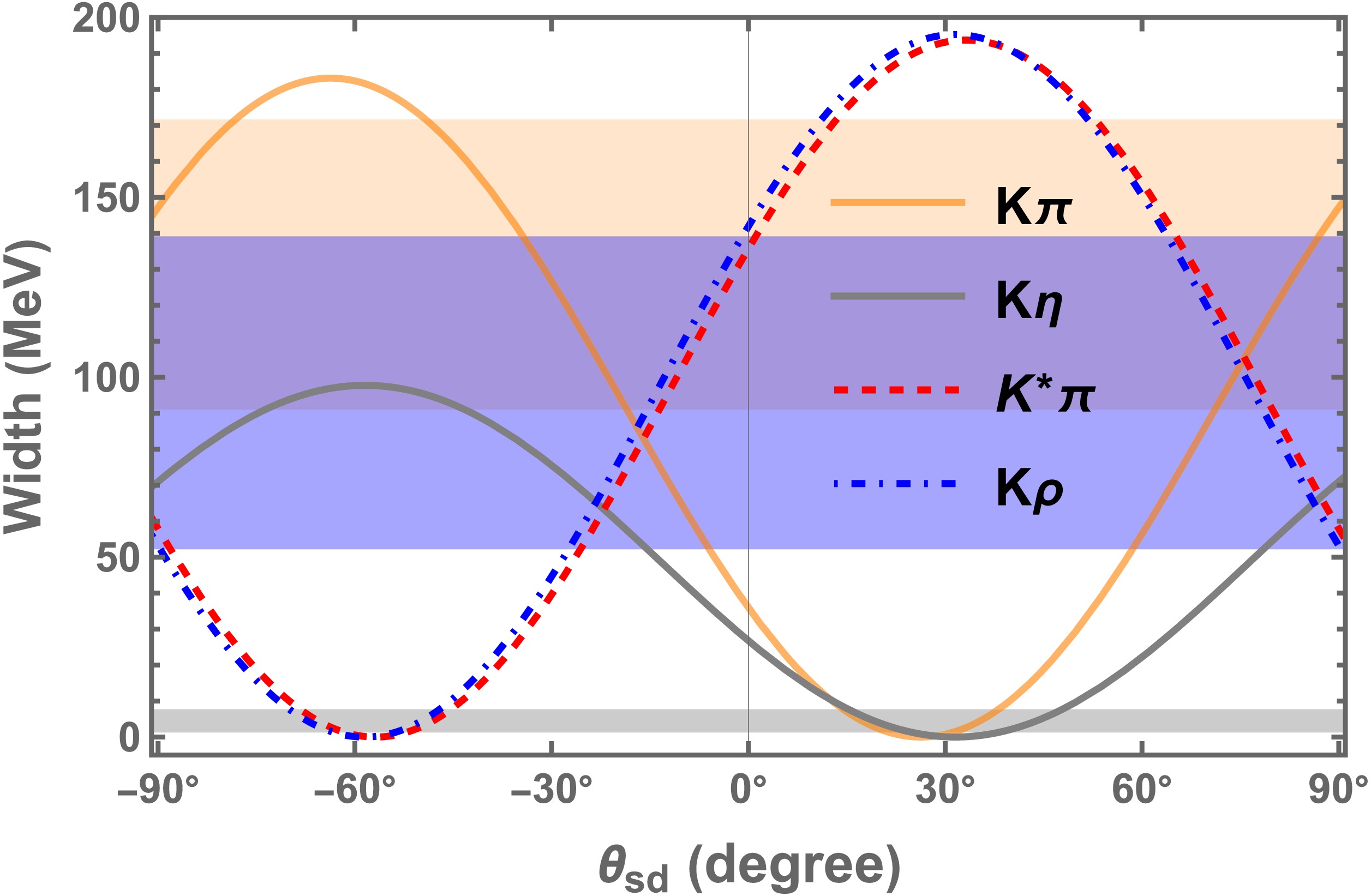
Figure 3. (color online) The orange solid line, gray solid line, red dashed line, and blue dot-dashed line represent the variations in the partial decay widths of
$ K^*(1680) $ into the final states$ K\pi $ ,$ K\eta $ ,$ K^*\pi $ , and$ K\rho $ as functions of the mixing angle$ \theta_{sd} $ , respectively. The horizontal orange, gray, and blue bands represent the experimental ranges for the decays of$ K^*(1680) $ into$ K\pi $ ,$ K\eta $ , and$ K^*\pi $ ($ K\rho $ ), respectively. Since the partial widths of the$ K^*\pi $ and$ K\rho $ channels are very close, as shown in Table 3, we use the experimental data for$ K^*\pi $ for both channels to keep the figure concise.For the
$ |q\bar{q}(3^3S_1)\rangle-|q\bar{q}(1^3D_1)\rangle $ mixing, the much smaller coupling of$ |q\bar{q}(3^3S_1)\rangle $ to the PP and VP channels means that it will be impossible to explain the small partial width for the$ K\eta $ decay if the other channels can be explained. In short, one can conclude that the pure$ q\bar{q} $ scenario is not sufficient for interpreting the experimental data, although the data still bear large uncertainties. This makes it natural to introduce$ q\bar{q} $ and hybrid mixing as a possible solution. -
In Table 2, we list the extracted effective couplings in the QPC model by treating
$ K^*(1680) $ as a$ q\bar{q} $ vector state, namely, either$ |q\bar{q}(2^3S_1)\rangle $ ,$ |q\bar{q}(3^3S_1)\rangle $ , or$ |q\bar{q}(1^3D_1)\rangle $ . It can be seen that the radial excitation$ |q\bar{q}(3^3S_1)\rangle $ has rather small couplings to the PP and VP channels. As shown below, this implies that$ K^*(1680) $ is unlikely to be the$ |q\bar{q}(3^3S_1)\rangle $ state.$ K^+\pi^0 $ $ K^+\eta $ $ K^+\eta^{\prime} $ $ K^{*+}\pi^0 $ $ K^+\rho^0 $ $ K^+\omega $ $ K^+\phi $ $ K^{*+}\eta $ $g^{{\rm{QPC}}}(2^3S_1) $ 1.18 2.16 0.14 4.62 5.32 5.35 5.64 0.93 $g^{{\rm{QPC}}}(3^3S_1) $ 0.02 −0.23 −0.01 −1.16 −1.54 −1.57 −2.06 −0.27 $g^{{\rm{QPC}}}(1^3D_1) $ 2.39 3.52 0.57 −3.02 −3.25 −3.27 −2.79 −1.12 $g^{{\rm{QPC}}}(1^3S_1)_1 $ −4.66 −7.12 0.29 −10.23 −11.26 −11.31 −0.68 −1.12 $g^{{\rm{QPC}}}(1^3S_1)_2 $ −3.14 −4.79 0.19 −6.88 −7.58 −7.59 −7.61 −0.46 Table 2. The coupling constants for the decays
$ K^*(1680)\to PP $ and VP were extracted using the QPC model, assuming that$ K^*(1680) $ is a pure$ |q\bar{q}(2^3S_1) \rangle $ ,$ |q\bar{q}(3^3S_1)\rangle $ , or$ |q\bar{q}(1^3D_1) \rangle $ state. Given that$ K^*(1680) $ is the lowest-energy hybrid, the$ q\bar{q} $ component should be in the ground state$ 1^3S_1 $ . The corresponding coupling constants, extracted in the QPC model at the mass of$ K^*(1680) $ , are listed in the fifth and sixth rows, where the subscripts "1" and "2" denote the different values$ \gamma_1 = 10.4 $ and$ \gamma_2 = 7 $ adopted in the calculation, respectively.More specifically, the corresponding partial decay widths are listed in Table 3, where they can be compared with the experimental data. The calculated partial widths obtained by assigning
$ K^*(1680) $ to the pure$ |q\bar{q}(2^3S_1)\rangle $ and$ |q\bar{q}(3^3S_1)\rangle $ states exhibit significant discrepancies with the experimental data. For$ |q\bar{q}(2^3S_1)\rangle\to K^*\pi $ and$ K\rho $ , the calculated values can be considered to be in agreement with the experimental data within the uncertainties. However, the partial widths for$ K^*(1680)\to K\pi $ and$ K\eta $ clearly cannot be explained by the transitions of$ |q\bar{q}(2^3S_1)\rangle\to K\pi $ and$ K\eta $ , respectively. With the assignment of a pure$ |q\bar{q}(3^3S_1)\rangle $ state, almost none of the decay channels can be accounted for. In contrast, with the assignment of a pure$ |q\bar{q}(1^3D_1)\rangle $ state, better agreement with the experimental data can be achieved in the$ K\pi $ ,$ K^*\pi $ , and$ K\rho $ channels. The results with$ \gamma_1= 10.4 $ adopted for the QPC coupling are also consistent with those reported in Ref. [31]. However, the calculated partial width for the$ K\eta $ channel is one order of magnitude larger than the data. Moreover, the partial widths of the$ K^*\pi $ and$ K\rho $ channels are close to the lower bounds of the uncertainty ranges.Modes $ K\pi $ $ K\eta $ $ K\eta^\prime $ $ K^*\pi $ $ K\rho $ $ K\omega $ $ K\phi $ $ K^*\eta $ Tot $ \chi^2 $ Expt. $ 123.84^{+53.32}_{-47.82} $ $ 4.48^{+5.84}_{-3.22} $ - $ 95.68^{+42.35}_{-43.39} $ $ 100.48^{+56.04}_{-38.95} $ - seen - $ 320\pm 110 $ - pure $ |q\bar{q}(2^3S_1)\rangle $ 35.95 26.76 0.03 135.77 142.02 46.90 16.62 0.76 404.82 - pure $ |q\bar{q}(3^3S_1)\rangle $ 0.008 0.31 $ \sim0 $ 8.62 12.00 4.02 2.22 0.06 27.24 - pure $ |q\bar{q}(1^3D_1)\rangle $ 147.18 70.97 0.50 57.95 53.21 17.53 4.06 1.09 352.48 - $ |q\bar{q}(1^3D_1)\rangle+|q\bar{q}\tilde{g}\rangle^a $ $ 85.52\pm 7.07 $ $ 3.28\pm 4.68 $ $ 0.62\pm 0.02 $ $ 109.35\pm 7.13 $ $ 101.55\pm 6.73 $ $ 70.88\pm 8.76 $ $ 13.46\pm 1.49 $ $ 1.98\pm 0.13 $ $ 386.63\pm 21.85 $ 1.12 $ |q\bar{q}(1^3D_1)\rangle+|q\bar{q}\tilde{g}\rangle^b $ $ 94.31\pm 5.48 $ $ 3.84\pm 4.54 $ $ 0.62\pm 0.02 $ $ 100.74\pm 5.21 $ $ 83.43\pm 4.91 $ $ 69.56\pm 7.59 $ $ 12.80\pm 1.23 $ $ 2.02\pm 0.12 $ $ 377.31\pm 18.11 $ 0.67 $ |q\bar{q}(1^3D_1)\rangle+|q\bar{q}\tilde{g}\rangle^c $ $ 101.14\pm 4.57 $ $ 4.10\pm 4.46 $ $ 0.62\pm 0.02 $ $ 94.39\pm 4.15 $ $ 87.45\pm 3.91 $ $ 68.26\pm 6.99 $ $ 12.28\pm 1.08 $ $ 2.03\pm 0.11 $ $ 370.27\pm 16.13 $ 0.49 $ |q\bar{q}(1^3D_1)\rangle+|q\bar{q}\tilde{g}\rangle^d $ $ 208.67\pm 8.25 $ $ 7.17\pm 4.13 $ $ 0.50\pm 0.01 $ $ 23.39\pm 3.66 $ $ 21.01\pm 3.39 $ $ 25.36\pm 1.06 $ $ 3.31\pm 0.11 $ $ 1.55\pm 0.07 $ $ 290.95\pm 1.91 $ 8.88 Table 3. The partial decay widths (in MeV) are calculated based on different scenarios for
$ K^*(1680) $ . The experimental results are listed in the second row. The values in the third, fourth, and fifth rows are obtained by treating$ K^*(1680) $ as a pure$ q\bar{q} $ state. The values in the sixth, seventh, eighth, and ninth rows are the results obtained by considering the mixing between the$ 1^3D_1 $ state and the hybrid state$ |q\bar{q}\tilde{g}\rangle $ . The superscripts$ a,\ b,\ c $ , and d on$ |q\bar{q}\tilde{g}\rangle $ correspond to the best-fitting results for ζ when δ takes the different values of$ 0.8,\ 1.0,\ 1.2 $ , and$ -0.8 $ , respectively. The last column shows the chi-square ($ \chi^2 $ ) values for the four fitting schemes.These results show that
$ K^*(1680) $ can hardly be interpreted as either a radial excitation state or a D-wave vector state. One may wonder whether$ S-D $ mixing can provide a solution. This appears highly unlikely, as indicated by the pure-state calculations. For the$ |q\bar{q}(2^3S_1)\rangle- |q\bar{q}(1^3D_1)\rangle $ mixing, if the S-wave is dominant, constructive interference from the D-wave in the PP channel would be required. This would lead to an even larger partial width for the$ K\eta $ channel and would contradict the data. If the D-wave is dominant, destructive interference from the S-wave would be required to satisfy the$ K\pi $ channel. However, a smaller and destructive S-wave component would still result in a large partial decay width for the$ K\eta $ channel.To quantify the
$ S-D $ mixing effects, we consider the physical states$ K^*(1410) $ and$ K^*(1680) $ as mixtures of the$ 1^3D_1 $ and$ 2^3S_1 $ states, similar to Ref. [31], i.e.,$ \begin{aligned} \begin{pmatrix} |K^*(1410)\rangle\\ |K^*(1680)\rangle \end{pmatrix}=\begin{pmatrix} {\rm{cos}}\theta_{sd}&{\rm{sin}}\theta_{sd}\\ -{\rm{sin}}\theta_{sd}&{\rm{cos}}\theta_{sd} \end{pmatrix}\begin{pmatrix} |1^3D_1\rangle\\ |2^3S_1\rangle \end{pmatrix}, \end{aligned} $
(30) where
$ \theta_{sd} $ denotes the mixing angle. The$ \theta_{sd} $ dependence of the partial decay widths for the$ \pi $ ,$ K\eta $ ,$ K^*\pi $ , and$ K\rho $ channels of$ K^*(1680) $ is presented in Fig. 3. The results show that no reasonable value or range of the mixing angle$ \theta_{sd} $ can simultaneously describe the experimental data for these four channels, even considering the large experimental uncertainties. This suggests that$ S-D $ mixing is insufficient to account for the data. In Ref. [31], it was suggested that, to explain the experimental total width of$ K^*(1410) $ , the mixing angle$ \theta_{sd} $ should be either$ -90^{\circ} $ or$ 90^{\circ} $ . This supports the scenario in which$ K^*(1410) $ is a pure$ 2^3S_1 $ state, and thus$ K^*(1680) $ would be a pure$ 1^3D_1 $ state. However, the small width of the$ K\eta $ channel cannot be explained in this picture. Nevertheless, various pieces of evidence indicate that$ S-D $ mixing cannot explain the decay pattern of$ K^*(1680) $ .
Figure 3. (color online) The orange solid line, gray solid line, red dashed line, and blue dot-dashed line represent the variations in the partial decay widths of
$ K^*(1680) $ into the final states$ K\pi $ ,$ K\eta $ ,$ K^*\pi $ , and$ K\rho $ as functions of the mixing angle$ \theta_{sd} $ , respectively. The horizontal orange, gray, and blue bands represent the experimental ranges for the decays of$ K^*(1680) $ into$ K\pi $ ,$ K\eta $ , and$ K^*\pi $ ($ K\rho $ ), respectively. Since the partial widths of the$ K^*\pi $ and$ K\rho $ channels are very close, as shown in Table 3, we use the experimental data for$ K^*\pi $ for both channels to keep the figure concise.For the
$ |q\bar{q}(3^3S_1)\rangle-|q\bar{q}(1^3D_1)\rangle $ mixing, the much smaller coupling of$ |q\bar{q}(3^3S_1)\rangle $ to the PP and VP channels means that it will be impossible to explain the small partial width for the$ K\eta $ decay if the other channels can be explained. In short, one can conclude that the pure$ q\bar{q} $ scenario is not sufficient for interpreting the experimental data, although the data still bear large uncertainties. This makes it natural to introduce$ q\bar{q} $ and hybrid mixing as a possible solution. -
In Table 2, we list the extracted effective couplings in the QPC model by treating
$ K^*(1680) $ as a$ q\bar{q} $ vector state, namely, either$ |q\bar{q}(2^3S_1)\rangle $ ,$ |q\bar{q}(3^3S_1)\rangle $ , or$ |q\bar{q}(1^3D_1)\rangle $ . It can be seen that the radial excitation$ |q\bar{q}(3^3S_1)\rangle $ has rather small couplings to the PP and VP channels. As shown below, this implies that$ K^*(1680) $ is unlikely to be the$ |q\bar{q}(3^3S_1)\rangle $ state.$ K^+\pi^0 $ $ K^+\eta $ $ K^+\eta^{\prime} $ $ K^{*+}\pi^0 $ $ K^+\rho^0 $ $ K^+\omega $ $ K^+\phi $ $ K^{*+}\eta $ $g^{{\rm{QPC}}}(2^3S_1) $ 1.18 2.16 0.14 4.62 5.32 5.35 5.64 0.93 $g^{{\rm{QPC}}}(3^3S_1) $ 0.02 −0.23 −0.01 −1.16 −1.54 −1.57 −2.06 −0.27 $g^{{\rm{QPC}}}(1^3D_1) $ 2.39 3.52 0.57 −3.02 −3.25 −3.27 −2.79 −1.12 $g^{{\rm{QPC}}}(1^3S_1)_1 $ −4.66 −7.12 0.29 −10.23 −11.26 −11.31 −0.68 −1.12 $g^{{\rm{QPC}}}(1^3S_1)_2 $ −3.14 −4.79 0.19 −6.88 −7.58 −7.59 −7.61 −0.46 Table 2. The coupling constants for the decays
$ K^*(1680)\to PP $ and VP were extracted using the QPC model, assuming that$ K^*(1680) $ is a pure$ |q\bar{q}(2^3S_1) \rangle $ ,$ |q\bar{q}(3^3S_1)\rangle $ , or$ |q\bar{q}(1^3D_1) \rangle $ state. Given that$ K^*(1680) $ is the lowest-energy hybrid, the$ q\bar{q} $ component should be in the ground state$ 1^3S_1 $ . The corresponding coupling constants, extracted in the QPC model at the mass of$ K^*(1680) $ , are listed in the fifth and sixth rows, where the subscripts "1" and "2" denote the different values$ \gamma_1 = 10.4 $ and$ \gamma_2 = 7 $ adopted in the calculation, respectively.More specifically, the corresponding partial decay widths are listed in Table 3, where they can be compared with the experimental data. The calculated partial widths obtained by assigning
$ K^*(1680) $ to the pure$ |q\bar{q}(2^3S_1)\rangle $ and$ |q\bar{q}(3^3S_1)\rangle $ states exhibit significant discrepancies with the experimental data. For$ |q\bar{q}(2^3S_1)\rangle\to K^*\pi $ and$ K\rho $ , the calculated values can be considered to be in agreement with the experimental data within the uncertainties. However, the partial widths for$ K^*(1680)\to K\pi $ and$ K\eta $ clearly cannot be explained by the transitions of$ |q\bar{q}(2^3S_1)\rangle\to K\pi $ and$ K\eta $ , respectively. With the assignment of a pure$ |q\bar{q}(3^3S_1)\rangle $ state, almost none of the decay channels can be accounted for. In contrast, with the assignment of a pure$ |q\bar{q}(1^3D_1)\rangle $ state, better agreement with the experimental data can be achieved in the$ K\pi $ ,$ K^*\pi $ , and$ K\rho $ channels. The results with$ \gamma_1= 10.4 $ adopted for the QPC coupling are also consistent with those reported in Ref. [31]. However, the calculated partial width for the$ K\eta $ channel is one order of magnitude larger than the data. Moreover, the partial widths of the$ K^*\pi $ and$ K\rho $ channels are close to the lower bounds of the uncertainty ranges.Modes $ K\pi $ $ K\eta $ $ K\eta^\prime $ $ K^*\pi $ $ K\rho $ $ K\omega $ $ K\phi $ $ K^*\eta $ Tot $ \chi^2 $ Expt. $ 123.84^{+53.32}_{-47.82} $ $ 4.48^{+5.84}_{-3.22} $ - $ 95.68^{+42.35}_{-43.39} $ $ 100.48^{+56.04}_{-38.95} $ - seen - $ 320\pm 110 $ - pure $ |q\bar{q}(2^3S_1)\rangle $ 35.95 26.76 0.03 135.77 142.02 46.90 16.62 0.76 404.82 - pure $ |q\bar{q}(3^3S_1)\rangle $ 0.008 0.31 $ \sim0 $ 8.62 12.00 4.02 2.22 0.06 27.24 - pure $ |q\bar{q}(1^3D_1)\rangle $ 147.18 70.97 0.50 57.95 53.21 17.53 4.06 1.09 352.48 - $ |q\bar{q}(1^3D_1)\rangle+|q\bar{q}\tilde{g}\rangle^a $ $ 85.52\pm 7.07 $ $ 3.28\pm 4.68 $ $ 0.62\pm 0.02 $ $ 109.35\pm 7.13 $ $ 101.55\pm 6.73 $ $ 70.88\pm 8.76 $ $ 13.46\pm 1.49 $ $ 1.98\pm 0.13 $ $ 386.63\pm 21.85 $ 1.12 $ |q\bar{q}(1^3D_1)\rangle+|q\bar{q}\tilde{g}\rangle^b $ $ 94.31\pm 5.48 $ $ 3.84\pm 4.54 $ $ 0.62\pm 0.02 $ $ 100.74\pm 5.21 $ $ 83.43\pm 4.91 $ $ 69.56\pm 7.59 $ $ 12.80\pm 1.23 $ $ 2.02\pm 0.12 $ $ 377.31\pm 18.11 $ 0.67 $ |q\bar{q}(1^3D_1)\rangle+|q\bar{q}\tilde{g}\rangle^c $ $ 101.14\pm 4.57 $ $ 4.10\pm 4.46 $ $ 0.62\pm 0.02 $ $ 94.39\pm 4.15 $ $ 87.45\pm 3.91 $ $ 68.26\pm 6.99 $ $ 12.28\pm 1.08 $ $ 2.03\pm 0.11 $ $ 370.27\pm 16.13 $ 0.49 $ |q\bar{q}(1^3D_1)\rangle+|q\bar{q}\tilde{g}\rangle^d $ $ 208.67\pm 8.25 $ $ 7.17\pm 4.13 $ $ 0.50\pm 0.01 $ $ 23.39\pm 3.66 $ $ 21.01\pm 3.39 $ $ 25.36\pm 1.06 $ $ 3.31\pm 0.11 $ $ 1.55\pm 0.07 $ $ 290.95\pm 1.91 $ 8.88 Table 3. The partial decay widths (in MeV) are calculated based on different scenarios for
$ K^*(1680) $ . The experimental results are listed in the second row. The values in the third, fourth, and fifth rows are obtained by treating$ K^*(1680) $ as a pure$ q\bar{q} $ state. The values in the sixth, seventh, eighth, and ninth rows are the results obtained by considering the mixing between the$ 1^3D_1 $ state and the hybrid state$ |q\bar{q}\tilde{g}\rangle $ . The superscripts$ a,\ b,\ c $ , and d on$ |q\bar{q}\tilde{g}\rangle $ correspond to the best-fitting results for ζ when δ takes the different values of$ 0.8,\ 1.0,\ 1.2 $ , and$ -0.8 $ , respectively. The last column shows the chi-square ($ \chi^2 $ ) values for the four fitting schemes.These results show that
$ K^*(1680) $ can hardly be interpreted as either a radial excitation state or a D-wave vector state. One may wonder whether$ S-D $ mixing can provide a solution. This appears highly unlikely, as indicated by the pure-state calculations. For the$ |q\bar{q}(2^3S_1)\rangle- |q\bar{q}(1^3D_1)\rangle $ mixing, if the S-wave is dominant, constructive interference from the D-wave in the PP channel would be required. This would lead to an even larger partial width for the$ K\eta $ channel and would contradict the data. If the D-wave is dominant, destructive interference from the S-wave would be required to satisfy the$ K\pi $ channel. However, a smaller and destructive S-wave component would still result in a large partial decay width for the$ K\eta $ channel.To quantify the
$ S-D $ mixing effects, we consider the physical states$ K^*(1410) $ and$ K^*(1680) $ as mixtures of the$ 1^3D_1 $ and$ 2^3S_1 $ states, similar to Ref. [31], i.e.,$ \begin{aligned} \begin{pmatrix} |K^*(1410)\rangle\\ |K^*(1680)\rangle \end{pmatrix}=\begin{pmatrix} {\rm{cos}}\theta_{sd}&{\rm{sin}}\theta_{sd}\\ -{\rm{sin}}\theta_{sd}&{\rm{cos}}\theta_{sd} \end{pmatrix}\begin{pmatrix} |1^3D_1\rangle\\ |2^3S_1\rangle \end{pmatrix}, \end{aligned} $
(30) where
$ \theta_{sd} $ denotes the mixing angle. The$ \theta_{sd} $ dependence of the partial decay widths for the$ \pi $ ,$ K\eta $ ,$ K^*\pi $ , and$ K\rho $ channels of$ K^*(1680) $ is presented in Fig. 3. The results show that no reasonable value or range of the mixing angle$ \theta_{sd} $ can simultaneously describe the experimental data for these four channels, even considering the large experimental uncertainties. This suggests that$ S-D $ mixing is insufficient to account for the data. In Ref. [31], it was suggested that, to explain the experimental total width of$ K^*(1410) $ , the mixing angle$ \theta_{sd} $ should be either$ -90^{\circ} $ or$ 90^{\circ} $ . This supports the scenario in which$ K^*(1410) $ is a pure$ 2^3S_1 $ state, and thus$ K^*(1680) $ would be a pure$ 1^3D_1 $ state. However, the small width of the$ K\eta $ channel cannot be explained in this picture. Nevertheless, various pieces of evidence indicate that$ S-D $ mixing cannot explain the decay pattern of$ K^*(1680) $ .
Figure 3. (color online) The orange solid line, gray solid line, red dashed line, and blue dot-dashed line represent the variations in the partial decay widths of
$ K^*(1680) $ into the final states$ K\pi $ ,$ K\eta $ ,$ K^*\pi $ , and$ K\rho $ as functions of the mixing angle$ \theta_{sd} $ , respectively. The horizontal orange, gray, and blue bands represent the experimental ranges for the decays of$ K^*(1680) $ into$ K\pi $ ,$ K\eta $ , and$ K^*\pi $ ($ K\rho $ ), respectively. Since the partial widths of the$ K^*\pi $ and$ K\rho $ channels are very close, as shown in Table 3, we use the experimental data for$ K^*\pi $ for both channels to keep the figure concise.For the
$ |q\bar{q}(3^3S_1)\rangle-|q\bar{q}(1^3D_1)\rangle $ mixing, the much smaller coupling of$ |q\bar{q}(3^3S_1)\rangle $ to the PP and VP channels means that it will be impossible to explain the small partial width for the$ K\eta $ decay if the other channels can be explained. In short, one can conclude that the pure$ q\bar{q} $ scenario is not sufficient for interpreting the experimental data, although the data still bear large uncertainties. This makes it natural to introduce$ q\bar{q} $ and hybrid mixing as a possible solution. -
In Table 2, we list the extracted effective couplings in the QPC model by treating
$ K^*(1680) $ as a$ q\bar{q} $ vector state, namely, either$ |q\bar{q}(2^3S_1)\rangle $ ,$ |q\bar{q}(3^3S_1)\rangle $ , or$ |q\bar{q}(1^3D_1)\rangle $ . It can be seen that the radial excitation$ |q\bar{q}(3^3S_1)\rangle $ has rather small couplings to the PP and VP channels. As shown below, this implies that$ K^*(1680) $ is unlikely to be the$ |q\bar{q}(3^3S_1)\rangle $ state.$ K^+\pi^0 $ $ K^+\eta $ $ K^+\eta^{\prime} $ $ K^{*+}\pi^0 $ $ K^+\rho^0 $ $ K^+\omega $ $ K^+\phi $ $ K^{*+}\eta $ $g^{{\rm{QPC}}}(2^3S_1) $ 1.18 2.16 0.14 4.62 5.32 5.35 5.64 0.93 $g^{{\rm{QPC}}}(3^3S_1) $ 0.02 −0.23 −0.01 −1.16 −1.54 −1.57 −2.06 −0.27 $g^{{\rm{QPC}}}(1^3D_1) $ 2.39 3.52 0.57 −3.02 −3.25 −3.27 −2.79 −1.12 $g^{{\rm{QPC}}}(1^3S_1)_1 $ −4.66 −7.12 0.29 −10.23 −11.26 −11.31 −0.68 −1.12 $g^{{\rm{QPC}}}(1^3S_1)_2 $ −3.14 −4.79 0.19 −6.88 −7.58 −7.59 −7.61 −0.46 Table 2. The coupling constants for the decays
$ K^*(1680)\to PP $ and VP were extracted using the QPC model, assuming that$ K^*(1680) $ is a pure$ |q\bar{q}(2^3S_1) \rangle $ ,$ |q\bar{q}(3^3S_1)\rangle $ , or$ |q\bar{q}(1^3D_1) \rangle $ state. Given that$ K^*(1680) $ is the lowest-energy hybrid, the$ q\bar{q} $ component should be in the ground state$ 1^3S_1 $ . The corresponding coupling constants, extracted in the QPC model at the mass of$ K^*(1680) $ , are listed in the fifth and sixth rows, where the subscripts "1" and "2" denote the different values$ \gamma_1 = 10.4 $ and$ \gamma_2 = 7 $ adopted in the calculation, respectively.More specifically, the corresponding partial decay widths are listed in Table 3, where they can be compared with the experimental data. The calculated partial widths obtained by assigning
$ K^*(1680) $ to the pure$ |q\bar{q}(2^3S_1)\rangle $ and$ |q\bar{q}(3^3S_1)\rangle $ states exhibit significant discrepancies with the experimental data. For$ |q\bar{q}(2^3S_1)\rangle\to K^*\pi $ and$ K\rho $ , the calculated values can be considered to be in agreement with the experimental data within the uncertainties. However, the partial widths for$ K^*(1680)\to K\pi $ and$ K\eta $ clearly cannot be explained by the transitions of$ |q\bar{q}(2^3S_1)\rangle\to K\pi $ and$ K\eta $ , respectively. With the assignment of a pure$ |q\bar{q}(3^3S_1)\rangle $ state, almost none of the decay channels can be accounted for. In contrast, with the assignment of a pure$ |q\bar{q}(1^3D_1)\rangle $ state, better agreement with the experimental data can be achieved in the$ K\pi $ ,$ K^*\pi $ , and$ K\rho $ channels. The results with$ \gamma_1= 10.4 $ adopted for the QPC coupling are also consistent with those reported in Ref. [31]. However, the calculated partial width for the$ K\eta $ channel is one order of magnitude larger than the data. Moreover, the partial widths of the$ K^*\pi $ and$ K\rho $ channels are close to the lower bounds of the uncertainty ranges.Modes $ K\pi $ $ K\eta $ $ K\eta^\prime $ $ K^*\pi $ $ K\rho $ $ K\omega $ $ K\phi $ $ K^*\eta $ Tot $ \chi^2 $ Expt. $ 123.84^{+53.32}_{-47.82} $ $ 4.48^{+5.84}_{-3.22} $ - $ 95.68^{+42.35}_{-43.39} $ $ 100.48^{+56.04}_{-38.95} $ - seen - $ 320\pm 110 $ - pure $ |q\bar{q}(2^3S_1)\rangle $ 35.95 26.76 0.03 135.77 142.02 46.90 16.62 0.76 404.82 - pure $ |q\bar{q}(3^3S_1)\rangle $ 0.008 0.31 $ \sim0 $ 8.62 12.00 4.02 2.22 0.06 27.24 - pure $ |q\bar{q}(1^3D_1)\rangle $ 147.18 70.97 0.50 57.95 53.21 17.53 4.06 1.09 352.48 - $ |q\bar{q}(1^3D_1)\rangle+|q\bar{q}\tilde{g}\rangle^a $ $ 85.52\pm 7.07 $ $ 3.28\pm 4.68 $ $ 0.62\pm 0.02 $ $ 109.35\pm 7.13 $ $ 101.55\pm 6.73 $ $ 70.88\pm 8.76 $ $ 13.46\pm 1.49 $ $ 1.98\pm 0.13 $ $ 386.63\pm 21.85 $ 1.12 $ |q\bar{q}(1^3D_1)\rangle+|q\bar{q}\tilde{g}\rangle^b $ $ 94.31\pm 5.48 $ $ 3.84\pm 4.54 $ $ 0.62\pm 0.02 $ $ 100.74\pm 5.21 $ $ 83.43\pm 4.91 $ $ 69.56\pm 7.59 $ $ 12.80\pm 1.23 $ $ 2.02\pm 0.12 $ $ 377.31\pm 18.11 $ 0.67 $ |q\bar{q}(1^3D_1)\rangle+|q\bar{q}\tilde{g}\rangle^c $ $ 101.14\pm 4.57 $ $ 4.10\pm 4.46 $ $ 0.62\pm 0.02 $ $ 94.39\pm 4.15 $ $ 87.45\pm 3.91 $ $ 68.26\pm 6.99 $ $ 12.28\pm 1.08 $ $ 2.03\pm 0.11 $ $ 370.27\pm 16.13 $ 0.49 $ |q\bar{q}(1^3D_1)\rangle+|q\bar{q}\tilde{g}\rangle^d $ $ 208.67\pm 8.25 $ $ 7.17\pm 4.13 $ $ 0.50\pm 0.01 $ $ 23.39\pm 3.66 $ $ 21.01\pm 3.39 $ $ 25.36\pm 1.06 $ $ 3.31\pm 0.11 $ $ 1.55\pm 0.07 $ $ 290.95\pm 1.91 $ 8.88 Table 3. The partial decay widths (in MeV) are calculated based on different scenarios for
$ K^*(1680) $ . The experimental results are listed in the second row. The values in the third, fourth, and fifth rows are obtained by treating$ K^*(1680) $ as a pure$ q\bar{q} $ state. The values in the sixth, seventh, eighth, and ninth rows are the results obtained by considering the mixing between the$ 1^3D_1 $ state and the hybrid state$ |q\bar{q}\tilde{g}\rangle $ . The superscripts$ a,\ b,\ c $ , and d on$ |q\bar{q}\tilde{g}\rangle $ correspond to the best-fitting results for ζ when δ takes the different values of$ 0.8,\ 1.0,\ 1.2 $ , and$ -0.8 $ , respectively. The last column shows the chi-square ($ \chi^2 $ ) values for the four fitting schemes.These results show that
$ K^*(1680) $ can hardly be interpreted as either a radial excitation state or a D-wave vector state. One may wonder whether$ S-D $ mixing can provide a solution. This appears highly unlikely, as indicated by the pure-state calculations. For the$ |q\bar{q}(2^3S_1)\rangle- |q\bar{q}(1^3D_1)\rangle $ mixing, if the S-wave is dominant, constructive interference from the D-wave in the PP channel would be required. This would lead to an even larger partial width for the$ K\eta $ channel and would contradict the data. If the D-wave is dominant, destructive interference from the S-wave would be required to satisfy the$ K\pi $ channel. However, a smaller and destructive S-wave component would still result in a large partial decay width for the$ K\eta $ channel.To quantify the
$ S-D $ mixing effects, we consider the physical states$ K^*(1410) $ and$ K^*(1680) $ as mixtures of the$ 1^3D_1 $ and$ 2^3S_1 $ states, similar to Ref. [31], i.e.,$ \begin{aligned} \begin{pmatrix} |K^*(1410)\rangle\\ |K^*(1680)\rangle \end{pmatrix}=\begin{pmatrix} {\rm{cos}}\theta_{sd}&{\rm{sin}}\theta_{sd}\\ -{\rm{sin}}\theta_{sd}&{\rm{cos}}\theta_{sd} \end{pmatrix}\begin{pmatrix} |1^3D_1\rangle\\ |2^3S_1\rangle \end{pmatrix}, \end{aligned} $
(30) where
$ \theta_{sd} $ denotes the mixing angle. The$ \theta_{sd} $ dependence of the partial decay widths for the$ \pi $ ,$ K\eta $ ,$ K^*\pi $ , and$ K\rho $ channels of$ K^*(1680) $ is presented in Fig. 3. The results show that no reasonable value or range of the mixing angle$ \theta_{sd} $ can simultaneously describe the experimental data for these four channels, even considering the large experimental uncertainties. This suggests that$ S-D $ mixing is insufficient to account for the data. In Ref. [31], it was suggested that, to explain the experimental total width of$ K^*(1410) $ , the mixing angle$ \theta_{sd} $ should be either$ -90^{\circ} $ or$ 90^{\circ} $ . This supports the scenario in which$ K^*(1410) $ is a pure$ 2^3S_1 $ state, and thus$ K^*(1680) $ would be a pure$ 1^3D_1 $ state. However, the small width of the$ K\eta $ channel cannot be explained in this picture. Nevertheless, various pieces of evidence indicate that$ S-D $ mixing cannot explain the decay pattern of$ K^*(1680) $ .
Figure 3. (color online) The orange solid line, gray solid line, red dashed line, and blue dot-dashed line represent the variations in the partial decay widths of
$ K^*(1680) $ into the final states$ K\pi $ ,$ K\eta $ ,$ K^*\pi $ , and$ K\rho $ as functions of the mixing angle$ \theta_{sd} $ , respectively. The horizontal orange, gray, and blue bands represent the experimental ranges for the decays of$ K^*(1680) $ into$ K\pi $ ,$ K\eta $ , and$ K^*\pi $ ($ K\rho $ ), respectively. Since the partial widths of the$ K^*\pi $ and$ K\rho $ channels are very close, as shown in Table 3, we use the experimental data for$ K^*\pi $ for both channels to keep the figure concise.For the
$ |q\bar{q}(3^3S_1)\rangle-|q\bar{q}(1^3D_1)\rangle $ mixing, the much smaller coupling of$ |q\bar{q}(3^3S_1)\rangle $ to the PP and VP channels means that it will be impossible to explain the small partial width for the$ K\eta $ decay if the other channels can be explained. In short, one can conclude that the pure$ q\bar{q} $ scenario is not sufficient for interpreting the experimental data, although the data still bear large uncertainties. This makes it natural to introduce$ q\bar{q} $ and hybrid mixing as a possible solution. -
As discussed earlier, the hybrid decays into PP and VP via Fig. 1 (a) can be described by the QPC model, since the quark pair created by the gluelump will involve multiple soft-gluon exchanges, which ultimately lead to behavior similar to that of the
$ ^3P_0 $ decay. This makes the process in Fig. 1 (a) indistinguishable from that of an initial$ |1^3S_1(q\bar{q})\rangle $ . Note that the effective coupling$ g_1 $ is extracted by matching it to the QPC model and by assuming that it is connected to the coupling of the ground state$ |1^3S_1(q\bar{q})\rangle $ to PP and$ VV $ , but with the mass set to that of the$ K^*(1680) $ . However, since the physical mass, i.e., the mass of$ K^*(1680) $ , is far from that of the ground-state vector meson, this suggests that some suppression effects, such as off-shell form factors, should be present. In this sense, the coupling$ \gamma_2 $ defined in the QPC model (in connection with the effective coupling$ g_1 $ ) should not be larger than the ground-state$ q\bar{q} $ coupling$ \gamma_1 $ adopted in the QPC model. Furthermore, the hybrid coupling in the collinear mode is correlated with the$ q\bar{q} $ -hybrid mixing angle through the wave function. Owing to the lack of further constraints from either experiment or theory, we have to survey the correlation among these three parameters, i.e.,$ \gamma_2 $ , δ, and ζ.To proceed, we assume that the
$ q\bar{q} $ component in the$ K^*(1680) $ wave function is$ |q\bar{q}(1^3D_1)\rangle $ , which mixes with the hybrid component. With the$ K^*(1680) $ wave function$ |K^*(1680)\rangle=\cos\zeta |q\bar{q}(1^3D_1)\rangle+\sin\zeta |q\bar{q}\tilde{g}\rangle $ , the transition amplitude is described by Eq. (22), where the transition of the$ |q\bar{q}(1^3D_1)\rangle $ component is described by the QPC model, while the decay of the hybrid component is parametrized by the FT model, as formulated earlier. It should be noted again that the collinear mode can be connected to the ground-state$ q\bar{q} $ decay in the QPC model instead of to the excited states. Therefore, when implementing the QPC model to describe the transition$ |q\bar{q}\tilde{g}\rangle\to PP $ and VP via the collinear mode, its analogue in the QPC model is the$ |q\bar{q}(1^3S_1)\rangle $ configuration, which requires$ \gamma_2<\gamma_1 $ .With
$ \gamma_1= 10.4 $ adopted for the QPC coupling, the partial decay widths of the pure$ |q\bar{q}(1^3D_1)\rangle $ state are listed in Table 3. Actually, since the term from Fig. 1 (b) contributes only to channels containing isoscalar states, e.g.,$ K\eta $ ,$ K^*\eta $ , etc., the correlation between$ \gamma_2 $ and ζ can be investigated in decay channels that do not involve isoscalar final states, i.e.,$ K\pi $ ,$ K^*\pi $ , and$ K\rho $ . In principle, one can first determine$ \gamma_2 \ (<\gamma_1) $ and ζ by fitting the data for the$ K\pi $ ,$ K^*\pi $ , and$ K\rho $ decay channels. Then, with$ \gamma_2 $ and ζ fixed, the coupling ratio δ can be determined from the$ K\eta $ channel.Thus, instead of determining
$ \gamma_2 $ and ζ first, we first restrict the range of δ by arguing that$ |\delta|\simeq 1 $ . Our numerical study shows that the best parameter space can be obtained with$ \delta\simeq 1.2 $ and$ \gamma_2 <\gamma_1 $ . In Fig. 4, we show the correlation between$ \gamma_2 $ and ζ by fixing$ \delta=1.2 $ . For different values of$ \gamma_2=5, \ 6, \ 7, \ 8, \ 9 $ , the mixing angle ζ is determined by fitting the four measured channels. Fig. 4 (a) shows that, with increasing$ \gamma_2 $ , the mixing angle ζ decreases, which reflects the correlation between$ \gamma_2 $ and ζ through the hybrid amplitude proportional to$ \gamma_2\sin\zeta $ . An obvious negative linear correlation indeed appears between ζ and$ \gamma_2 $ , as shown in Fig. 4. This correlation can be understood through Eq. (22), where, with an increased value of$ \gamma_2 $ , the amplitude$ {\cal{M}}^{\rm Tot}_{PP/PV} $ can remain almost unchanged by adopting a smaller mixing angle ζ. As a result, the decay widths shown in Fig. 4 (b) can remain almost unchanged as$ \gamma_2 $ and ζ vary in a correlated way. This suggests that$ \gamma_2 $ and ζ cannot be determined from the present experimental results.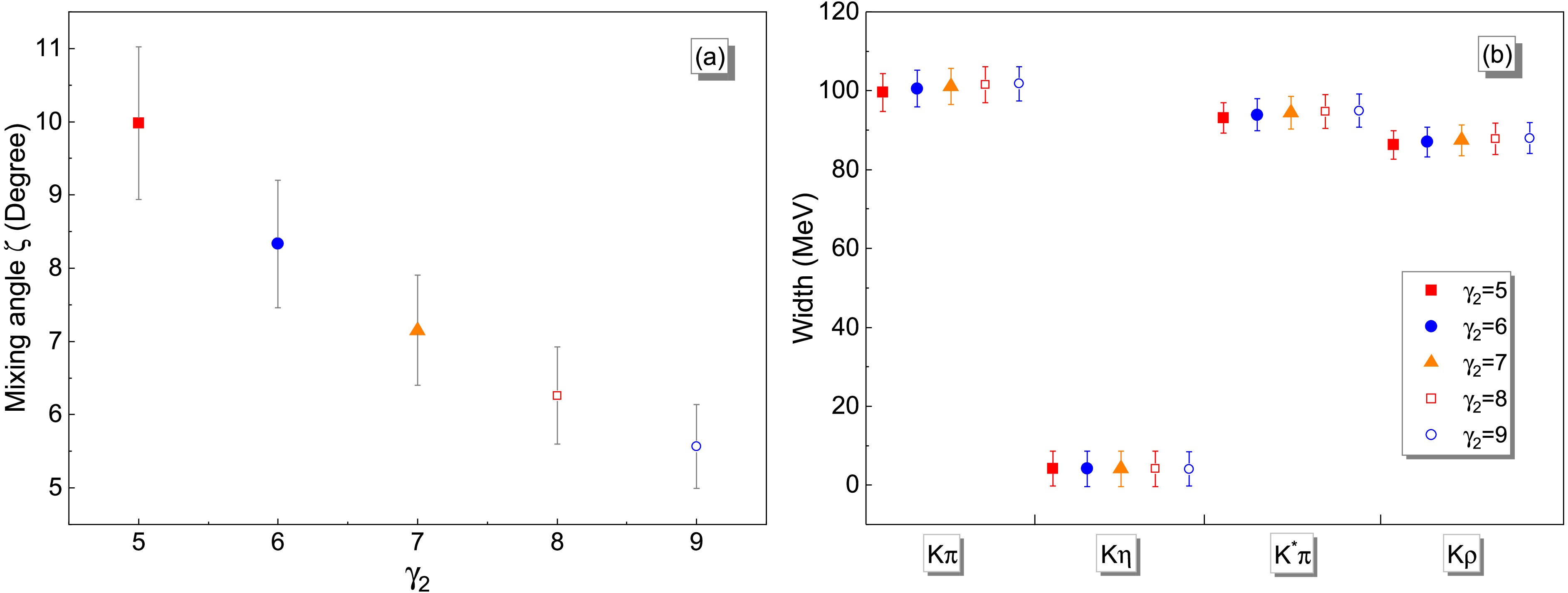
Figure 4. (color online) (a) The fitted mixing angle ζ for different values of
$ \gamma_2 $ :$ \gamma_2=5,\ 6,\ 7,\ 8, $ and$ 9 $ , with$ \delta=1.2 $ . (b) The partial decay widths for the four decay modes$ K\pi $ ,$ K\eta $ ,$ K^*\pi $ , and$ K\rho $ , fitted using the mixing angle ζ for$ \gamma_2=5,\ 6,\ 7,\ 8 $ , and$ 9 $ with$ \delta=1.2 $ .In Fig. 4 (b), we present the partial decay widths for different channels with the parameter values shown in Fig. 4 (a). The results do not show significant differences, which again indicates the correlation between
$ \gamma_2 $ and ζ for the fixed value of$ \delta=1.2 $ . Although the δ term contributes only to channels involving the isoscalar pseudoscalar final state, we can also see its impact on the numerical fit. In Table 3, we list the best-fit results for ζ when δ takes the different values of$ 0.8,\ 1.0,\ 1.2 $ , and$ -0.8 $ , which are labeled by the superscripts$ a,\ b,\ c $ , and d, respectively. The fitting quality is shown by the$ \chi^2 $ value in the last column.As shown in Table 3, the best fit is obtained for the case with
$ \gamma_2=7 $ and$ \delta=1.2 $ . This shows that hybrid mixing reduces the partial widths of the PP channels for the pure$ |q\bar{q}(1^3D_1)\rangle $ decay and enhances those of the VP channels. In particular, the$ K\eta $ channel receives destructive interference, and the partial width falls within the experimental range. It is interesting to note that the transition amplitudes of$ |q\bar{q}(1^3D_1)\rangle\to PP $ and VP have different signs arising from the spin factors. However, for the ground-state$ q\bar{q}(1^3S_1) $ , these two transitions have the same sign. This feature turns out to be crucial for accounting for the pattern of the$ K^*(1680)\to PP $ and VP decays. Note that$ S-D $ mixing alone cannot yield as good a fit as that from scheme "c'' in Table 3.From Fig. 4 (a), we obtain the fitted mixing angle
$ \zeta=7.15^{\circ} \pm0.76^{\circ} $ , which turns out to be rather small. This suggests that the behavior of$ K^*(1680) $ is still dominated by the conventional$ q\bar{q} $ configuration, while the hybrid component is quite small. However, as shown by our numerical survey, such a small hybrid component is crucial for describing the$ K^*(1680) $ decay pattern. -
As discussed earlier, the hybrid decays into PP and VP via Fig. 1 (a) can be described by the QPC model, since the quark pair created by the gluelump will involve multiple soft-gluon exchanges, which ultimately lead to behavior similar to that of the
$ ^3P_0 $ decay. This makes the process in Fig. 1 (a) indistinguishable from that of an initial$ |1^3S_1(q\bar{q})\rangle $ . Note that the effective coupling$ g_1 $ is extracted by matching it to the QPC model and by assuming that it is connected to the coupling of the ground state$ |1^3S_1(q\bar{q})\rangle $ to PP and$ VV $ , but with the mass set to that of the$ K^*(1680) $ . However, since the physical mass, i.e., the mass of$ K^*(1680) $ , is far from that of the ground-state vector meson, this suggests that some suppression effects, such as off-shell form factors, should be present. In this sense, the coupling$ \gamma_2 $ defined in the QPC model (in connection with the effective coupling$ g_1 $ ) should not be larger than the ground-state$ q\bar{q} $ coupling$ \gamma_1 $ adopted in the QPC model. Furthermore, the hybrid coupling in the collinear mode is correlated with the$ q\bar{q} $ -hybrid mixing angle through the wave function. Owing to the lack of further constraints from either experiment or theory, we have to survey the correlation among these three parameters, i.e.,$ \gamma_2 $ , δ, and ζ.To proceed, we assume that the
$ q\bar{q} $ component in the$ K^*(1680) $ wave function is$ |q\bar{q}(1^3D_1)\rangle $ , which mixes with the hybrid component. With the$ K^*(1680) $ wave function$ |K^*(1680)\rangle=\cos\zeta |q\bar{q}(1^3D_1)\rangle+\sin\zeta |q\bar{q}\tilde{g}\rangle $ , the transition amplitude is described by Eq. (22), where the transition of the$ |q\bar{q}(1^3D_1)\rangle $ component is described by the QPC model, while the decay of the hybrid component is parametrized by the FT model, as formulated earlier. It should be noted again that the collinear mode can be connected to the ground-state$ q\bar{q} $ decay in the QPC model instead of to the excited states. Therefore, when implementing the QPC model to describe the transition$ |q\bar{q}\tilde{g}\rangle\to PP $ and VP via the collinear mode, its analogue in the QPC model is the$ |q\bar{q}(1^3S_1)\rangle $ configuration, which requires$ \gamma_2<\gamma_1 $ .With
$ \gamma_1= 10.4 $ adopted for the QPC coupling, the partial decay widths of the pure$ |q\bar{q}(1^3D_1)\rangle $ state are listed in Table 3. Actually, since the term from Fig. 1 (b) contributes only to channels containing isoscalar states, e.g.,$ K\eta $ ,$ K^*\eta $ , etc., the correlation between$ \gamma_2 $ and ζ can be investigated in decay channels that do not involve isoscalar final states, i.e.,$ K\pi $ ,$ K^*\pi $ , and$ K\rho $ . In principle, one can first determine$ \gamma_2 \ (<\gamma_1) $ and ζ by fitting the data for the$ K\pi $ ,$ K^*\pi $ , and$ K\rho $ decay channels. Then, with$ \gamma_2 $ and ζ fixed, the coupling ratio δ can be determined from the$ K\eta $ channel.Thus, instead of determining
$ \gamma_2 $ and ζ first, we first restrict the range of δ by arguing that$ |\delta|\simeq 1 $ . Our numerical study shows that the best parameter space can be obtained with$ \delta\simeq 1.2 $ and$ \gamma_2 <\gamma_1 $ . In Fig. 4, we show the correlation between$ \gamma_2 $ and ζ by fixing$ \delta=1.2 $ . For different values of$ \gamma_2=5, \ 6, \ 7, \ 8, \ 9 $ , the mixing angle ζ is determined by fitting the four measured channels. Fig. 4 (a) shows that, with increasing$ \gamma_2 $ , the mixing angle ζ decreases, which reflects the correlation between$ \gamma_2 $ and ζ through the hybrid amplitude proportional to$ \gamma_2\sin\zeta $ . An obvious negative linear correlation indeed appears between ζ and$ \gamma_2 $ , as shown in Fig. 4. This correlation can be understood through Eq. (22), where, with an increased value of$ \gamma_2 $ , the amplitude$ {\cal{M}}^{\rm Tot}_{PP/PV} $ can remain almost unchanged by adopting a smaller mixing angle ζ. As a result, the decay widths shown in Fig. 4 (b) can remain almost unchanged as$ \gamma_2 $ and ζ vary in a correlated way. This suggests that$ \gamma_2 $ and ζ cannot be determined from the present experimental results.
Figure 4. (color online) (a) The fitted mixing angle ζ for different values of
$ \gamma_2 $ :$ \gamma_2=5,\ 6,\ 7,\ 8, $ and$ 9 $ , with$ \delta=1.2 $ . (b) The partial decay widths for the four decay modes$ K\pi $ ,$ K\eta $ ,$ K^*\pi $ , and$ K\rho $ , fitted using the mixing angle ζ for$ \gamma_2=5,\ 6,\ 7,\ 8 $ , and$ 9 $ with$ \delta=1.2 $ .In Fig. 4 (b), we present the partial decay widths for different channels with the parameter values shown in Fig. 4 (a). The results do not show significant differences, which again indicates the correlation between
$ \gamma_2 $ and ζ for the fixed value of$ \delta=1.2 $ . Although the δ term contributes only to channels involving the isoscalar pseudoscalar final state, we can also see its impact on the numerical fit. In Table 3, we list the best-fit results for ζ when δ takes the different values of$ 0.8,\ 1.0,\ 1.2 $ , and$ -0.8 $ , which are labeled by the superscripts$ a,\ b,\ c $ , and d, respectively. The fitting quality is shown by the$ \chi^2 $ value in the last column.As shown in Table 3, the best fit is obtained for the case with
$ \gamma_2=7 $ and$ \delta=1.2 $ . This shows that hybrid mixing reduces the partial widths of the PP channels for the pure$ |q\bar{q}(1^3D_1)\rangle $ decay and enhances those of the VP channels. In particular, the$ K\eta $ channel receives destructive interference, and the partial width falls within the experimental range. It is interesting to note that the transition amplitudes of$ |q\bar{q}(1^3D_1)\rangle\to PP $ and VP have different signs arising from the spin factors. However, for the ground-state$ q\bar{q}(1^3S_1) $ , these two transitions have the same sign. This feature turns out to be crucial for accounting for the pattern of the$ K^*(1680)\to PP $ and VP decays. Note that$ S-D $ mixing alone cannot yield as good a fit as that from scheme "c'' in Table 3.From Fig. 4 (a), we obtain the fitted mixing angle
$ \zeta=7.15^{\circ} \pm0.76^{\circ} $ , which turns out to be rather small. This suggests that the behavior of$ K^*(1680) $ is still dominated by the conventional$ q\bar{q} $ configuration, while the hybrid component is quite small. However, as shown by our numerical survey, such a small hybrid component is crucial for describing the$ K^*(1680) $ decay pattern. -
As discussed earlier, the hybrid decays into PP and VP via Fig. 1 (a) can be described by the QPC model, since the quark pair created by the gluelump will involve multiple soft-gluon exchanges, which ultimately lead to behavior similar to that of the
$ ^3P_0 $ decay. This makes the process in Fig. 1 (a) indistinguishable from that of an initial$ |1^3S_1(q\bar{q})\rangle $ . Note that the effective coupling$ g_1 $ is extracted by matching it to the QPC model and by assuming that it is connected to the coupling of the ground state$ |1^3S_1(q\bar{q})\rangle $ to PP and$ VV $ , but with the mass set to that of the$ K^*(1680) $ . However, since the physical mass, i.e., the mass of$ K^*(1680) $ , is far from that of the ground-state vector meson, this suggests that some suppression effects, such as off-shell form factors, should be present. In this sense, the coupling$ \gamma_2 $ defined in the QPC model (in connection with the effective coupling$ g_1 $ ) should not be larger than the ground-state$ q\bar{q} $ coupling$ \gamma_1 $ adopted in the QPC model. Furthermore, the hybrid coupling in the collinear mode is correlated with the$ q\bar{q} $ -hybrid mixing angle through the wave function. Owing to the lack of further constraints from either experiment or theory, we have to survey the correlation among these three parameters, i.e.,$ \gamma_2 $ , δ, and ζ.To proceed, we assume that the
$ q\bar{q} $ component in the$ K^*(1680) $ wave function is$ |q\bar{q}(1^3D_1)\rangle $ , which mixes with the hybrid component. With the$ K^*(1680) $ wave function$ |K^*(1680)\rangle=\cos\zeta |q\bar{q}(1^3D_1)\rangle+\sin\zeta |q\bar{q}\tilde{g}\rangle $ , the transition amplitude is described by Eq. (22), where the transition of the$ |q\bar{q}(1^3D_1)\rangle $ component is described by the QPC model, while the decay of the hybrid component is parametrized by the FT model, as formulated earlier. It should be noted again that the collinear mode can be connected to the ground-state$ q\bar{q} $ decay in the QPC model instead of to the excited states. Therefore, when implementing the QPC model to describe the transition$ |q\bar{q}\tilde{g}\rangle\to PP $ and VP via the collinear mode, its analogue in the QPC model is the$ |q\bar{q}(1^3S_1)\rangle $ configuration, which requires$ \gamma_2<\gamma_1 $ .With
$ \gamma_1= 10.4 $ adopted for the QPC coupling, the partial decay widths of the pure$ |q\bar{q}(1^3D_1)\rangle $ state are listed in Table 3. Actually, since the term from Fig. 1 (b) contributes only to channels containing isoscalar states, e.g.,$ K\eta $ ,$ K^*\eta $ , etc., the correlation between$ \gamma_2 $ and ζ can be investigated in decay channels that do not involve isoscalar final states, i.e.,$ K\pi $ ,$ K^*\pi $ , and$ K\rho $ . In principle, one can first determine$ \gamma_2 \ (<\gamma_1) $ and ζ by fitting the data for the$ K\pi $ ,$ K^*\pi $ , and$ K\rho $ decay channels. Then, with$ \gamma_2 $ and ζ fixed, the coupling ratio δ can be determined from the$ K\eta $ channel.Thus, instead of determining
$ \gamma_2 $ and ζ first, we first restrict the range of δ by arguing that$ |\delta|\simeq 1 $ . Our numerical study shows that the best parameter space can be obtained with$ \delta\simeq 1.2 $ and$ \gamma_2 <\gamma_1 $ . In Fig. 4, we show the correlation between$ \gamma_2 $ and ζ by fixing$ \delta=1.2 $ . For different values of$ \gamma_2=5, \ 6, \ 7, \ 8, \ 9 $ , the mixing angle ζ is determined by fitting the four measured channels. Fig. 4 (a) shows that, with increasing$ \gamma_2 $ , the mixing angle ζ decreases, which reflects the correlation between$ \gamma_2 $ and ζ through the hybrid amplitude proportional to$ \gamma_2\sin\zeta $ . An obvious negative linear correlation indeed appears between ζ and$ \gamma_2 $ , as shown in Fig. 4. This correlation can be understood through Eq. (22), where, with an increased value of$ \gamma_2 $ , the amplitude$ {\cal{M}}^{\rm Tot}_{PP/PV} $ can remain almost unchanged by adopting a smaller mixing angle ζ. As a result, the decay widths shown in Fig. 4 (b) can remain almost unchanged as$ \gamma_2 $ and ζ vary in a correlated way. This suggests that$ \gamma_2 $ and ζ cannot be determined from the present experimental results.
Figure 4. (color online) (a) The fitted mixing angle ζ for different values of
$ \gamma_2 $ :$ \gamma_2=5,\ 6,\ 7,\ 8, $ and$ 9 $ , with$ \delta=1.2 $ . (b) The partial decay widths for the four decay modes$ K\pi $ ,$ K\eta $ ,$ K^*\pi $ , and$ K\rho $ , fitted using the mixing angle ζ for$ \gamma_2=5,\ 6,\ 7,\ 8 $ , and$ 9 $ with$ \delta=1.2 $ .In Fig. 4 (b), we present the partial decay widths for different channels with the parameter values shown in Fig. 4 (a). The results do not show significant differences, which again indicates the correlation between
$ \gamma_2 $ and ζ for the fixed value of$ \delta=1.2 $ . Although the δ term contributes only to channels involving the isoscalar pseudoscalar final state, we can also see its impact on the numerical fit. In Table 3, we list the best-fit results for ζ when δ takes the different values of$ 0.8,\ 1.0,\ 1.2 $ , and$ -0.8 $ , which are labeled by the superscripts$ a,\ b,\ c $ , and d, respectively. The fitting quality is shown by the$ \chi^2 $ value in the last column.As shown in Table 3, the best fit is obtained for the case with
$ \gamma_2=7 $ and$ \delta=1.2 $ . This shows that hybrid mixing reduces the partial widths of the PP channels for the pure$ |q\bar{q}(1^3D_1)\rangle $ decay and enhances those of the VP channels. In particular, the$ K\eta $ channel receives destructive interference, and the partial width falls within the experimental range. It is interesting to note that the transition amplitudes of$ |q\bar{q}(1^3D_1)\rangle\to PP $ and VP have different signs arising from the spin factors. However, for the ground-state$ q\bar{q}(1^3S_1) $ , these two transitions have the same sign. This feature turns out to be crucial for accounting for the pattern of the$ K^*(1680)\to PP $ and VP decays. Note that$ S-D $ mixing alone cannot yield as good a fit as that from scheme "c'' in Table 3.From Fig. 4 (a), we obtain the fitted mixing angle
$ \zeta=7.15^{\circ} \pm0.76^{\circ} $ , which turns out to be rather small. This suggests that the behavior of$ K^*(1680) $ is still dominated by the conventional$ q\bar{q} $ configuration, while the hybrid component is quite small. However, as shown by our numerical survey, such a small hybrid component is crucial for describing the$ K^*(1680) $ decay pattern. -
As discussed earlier, the hybrid decays into PP and VP via Fig. 1 (a) can be described by the QPC model, since the quark pair created by the gluelump will involve multiple soft-gluon exchanges, which ultimately lead to behavior similar to that of the
$ ^3P_0 $ decay. This makes the process in Fig. 1 (a) indistinguishable from that of an initial$ |1^3S_1(q\bar{q})\rangle $ . Note that the effective coupling$ g_1 $ is extracted by matching it to the QPC model and by assuming that it is connected to the coupling of the ground state$ |1^3S_1(q\bar{q})\rangle $ to PP and$ VV $ , but with the mass set to that of the$ K^*(1680) $ . However, since the physical mass, i.e., the mass of$ K^*(1680) $ , is far from that of the ground-state vector meson, this suggests that some suppression effects, such as off-shell form factors, should be present. In this sense, the coupling$ \gamma_2 $ defined in the QPC model (in connection with the effective coupling$ g_1 $ ) should not be larger than the ground-state$ q\bar{q} $ coupling$ \gamma_1 $ adopted in the QPC model. Furthermore, the hybrid coupling in the collinear mode is correlated with the$ q\bar{q} $ -hybrid mixing angle through the wave function. Owing to the lack of further constraints from either experiment or theory, we have to survey the correlation among these three parameters, i.e.,$ \gamma_2 $ , δ, and ζ.To proceed, we assume that the
$ q\bar{q} $ component in the$ K^*(1680) $ wave function is$ |q\bar{q}(1^3D_1)\rangle $ , which mixes with the hybrid component. With the$ K^*(1680) $ wave function$ |K^*(1680)\rangle=\cos\zeta |q\bar{q}(1^3D_1)\rangle+\sin\zeta |q\bar{q}\tilde{g}\rangle $ , the transition amplitude is described by Eq. (22), where the transition of the$ |q\bar{q}(1^3D_1)\rangle $ component is described by the QPC model, while the decay of the hybrid component is parametrized by the FT model, as formulated earlier. It should be noted again that the collinear mode can be connected to the ground-state$ q\bar{q} $ decay in the QPC model instead of to the excited states. Therefore, when implementing the QPC model to describe the transition$ |q\bar{q}\tilde{g}\rangle\to PP $ and VP via the collinear mode, its analogue in the QPC model is the$ |q\bar{q}(1^3S_1)\rangle $ configuration, which requires$ \gamma_2<\gamma_1 $ .With
$ \gamma_1= 10.4 $ adopted for the QPC coupling, the partial decay widths of the pure$ |q\bar{q}(1^3D_1)\rangle $ state are listed in Table 3. Actually, since the term from Fig. 1 (b) contributes only to channels containing isoscalar states, e.g.,$ K\eta $ ,$ K^*\eta $ , etc., the correlation between$ \gamma_2 $ and ζ can be investigated in decay channels that do not involve isoscalar final states, i.e.,$ K\pi $ ,$ K^*\pi $ , and$ K\rho $ . In principle, one can first determine$ \gamma_2 \ (<\gamma_1) $ and ζ by fitting the data for the$ K\pi $ ,$ K^*\pi $ , and$ K\rho $ decay channels. Then, with$ \gamma_2 $ and ζ fixed, the coupling ratio δ can be determined from the$ K\eta $ channel.Thus, instead of determining
$ \gamma_2 $ and ζ first, we first restrict the range of δ by arguing that$ |\delta|\simeq 1 $ . Our numerical study shows that the best parameter space can be obtained with$ \delta\simeq 1.2 $ and$ \gamma_2 <\gamma_1 $ . In Fig. 4, we show the correlation between$ \gamma_2 $ and ζ by fixing$ \delta=1.2 $ . For different values of$ \gamma_2=5, \ 6, \ 7, \ 8, \ 9 $ , the mixing angle ζ is determined by fitting the four measured channels. Fig. 4 (a) shows that, with increasing$ \gamma_2 $ , the mixing angle ζ decreases, which reflects the correlation between$ \gamma_2 $ and ζ through the hybrid amplitude proportional to$ \gamma_2\sin\zeta $ . An obvious negative linear correlation indeed appears between ζ and$ \gamma_2 $ , as shown in Fig. 4. This correlation can be understood through Eq. (22), where, with an increased value of$ \gamma_2 $ , the amplitude$ {\cal{M}}^{\rm Tot}_{PP/PV} $ can remain almost unchanged by adopting a smaller mixing angle ζ. As a result, the decay widths shown in Fig. 4 (b) can remain almost unchanged as$ \gamma_2 $ and ζ vary in a correlated way. This suggests that$ \gamma_2 $ and ζ cannot be determined from the present experimental results.
Figure 4. (color online) (a) The fitted mixing angle ζ for different values of
$ \gamma_2 $ :$ \gamma_2=5,\ 6,\ 7,\ 8, $ and$ 9 $ , with$ \delta=1.2 $ . (b) The partial decay widths for the four decay modes$ K\pi $ ,$ K\eta $ ,$ K^*\pi $ , and$ K\rho $ , fitted using the mixing angle ζ for$ \gamma_2=5,\ 6,\ 7,\ 8 $ , and$ 9 $ with$ \delta=1.2 $ .In Fig. 4 (b), we present the partial decay widths for different channels with the parameter values shown in Fig. 4 (a). The results do not show significant differences, which again indicates the correlation between
$ \gamma_2 $ and ζ for the fixed value of$ \delta=1.2 $ . Although the δ term contributes only to channels involving the isoscalar pseudoscalar final state, we can also see its impact on the numerical fit. In Table 3, we list the best-fit results for ζ when δ takes the different values of$ 0.8,\ 1.0,\ 1.2 $ , and$ -0.8 $ , which are labeled by the superscripts$ a,\ b,\ c $ , and d, respectively. The fitting quality is shown by the$ \chi^2 $ value in the last column.As shown in Table 3, the best fit is obtained for the case with
$ \gamma_2=7 $ and$ \delta=1.2 $ . This shows that hybrid mixing reduces the partial widths of the PP channels for the pure$ |q\bar{q}(1^3D_1)\rangle $ decay and enhances those of the VP channels. In particular, the$ K\eta $ channel receives destructive interference, and the partial width falls within the experimental range. It is interesting to note that the transition amplitudes of$ |q\bar{q}(1^3D_1)\rangle\to PP $ and VP have different signs arising from the spin factors. However, for the ground-state$ q\bar{q}(1^3S_1) $ , these two transitions have the same sign. This feature turns out to be crucial for accounting for the pattern of the$ K^*(1680)\to PP $ and VP decays. Note that$ S-D $ mixing alone cannot yield as good a fit as that from scheme "c'' in Table 3.From Fig. 4 (a), we obtain the fitted mixing angle
$ \zeta=7.15^{\circ} \pm0.76^{\circ} $ , which turns out to be rather small. This suggests that the behavior of$ K^*(1680) $ is still dominated by the conventional$ q\bar{q} $ configuration, while the hybrid component is quite small. However, as shown by our numerical survey, such a small hybrid component is crucial for describing the$ K^*(1680) $ decay pattern. -
The extracted small mixing angle
$ \zeta=7.15^{\circ} \pm0.76^{\circ} $ provides further insight into the$ q\bar{q} $ -hybrid mixing in the vector strange sector. More generally, we can express the eigenvalue equation for two-configuration mixing as$ \begin{aligned} \left(\begin{array}{cc} \hat{H}_q & \hat{H}_\Delta \\ \hat{H}_\Delta & \hat{H}_h \end{array}\right) \left(\begin{array}{c} \alpha \psi_q \\ \beta\psi_h \end{array}\right) &= E\left( \begin{array}{c} \alpha \psi_q \\ \beta\psi_h \end{array}\right) \ , \end{aligned} $
(31) where
$ \hat{H}_q $ and$ \hat{H}_h $ are the Hamiltonians for the pure$ q\bar{q} $ ($ \psi_q $ ) and pure hybrid ($ \psi_h $ ) systems, respectively;$ \hat{H}_\Delta $ is the transition operator mediating transitions between$ \psi_q $ and$ \psi_h $ ; and α and β are the probability amplitudes for the physical state to be in the pure states$ \psi_q $ and$ \psi_h $ , respectively. The normalisation condition requires$ \alpha^2+\beta^2=1 $ .Given the eigenvalues
$ E_q\equiv \langle \psi_q|\hat{H}_q|\psi_q\rangle $ and$ E_h\equiv \langle \psi_h|\hat{H}_h|\psi_h\rangle $ , and the transition amplitude$ \Delta\equiv \langle \psi_q|\hat{H}_\Delta|\psi_h\rangle= \langle \psi_h|\hat{H}_\Delta|\psi_q\rangle $ , the eigenvalue equation can be written as$ \begin{aligned} \left(\begin{array}{cc} E_q & \Delta \\ \Delta & E_h \end{array}\right) \left(\begin{array}{c} \alpha \\ \beta \end{array}\right) &= E\left( \begin{array}{c} \alpha \\ \beta \end{array}\right) \ , \end{aligned} $
(32) whose eigenvalue is determined by setting the determinant of the coefficient matrix to zero
$ \begin{aligned} E&=\frac 12\left[(E_q+E_h)\pm\sqrt{(E_q+E_h)^2-4(E_q E_h-\Delta^2)}\right] \ , \end{aligned} $
(33) where we define
$ E_L $ and$ E_H $ as the lower ("−") and higher ("+") solutions, respectively. Substituting these two solutions back into the eigenvalue equation, we obtain the physical wave function$ |\Psi\rangle=\alpha |\psi_q\rangle+\beta|\psi_h\rangle $ .In our convention, the extracted physical state is expressed as
$ |K^*(1680)\rangle=\cos\zeta |q\bar{q}(1^3D_1)\rangle+\sin\zeta |q\bar{q}\tilde{g}\rangle $ , where$ \psi_q=|q\bar{q}(1^3D_1)\rangle $ and$ \psi_h=|q\bar{q}\tilde{g}\rangle $ , with$ \alpha=\cos\zeta $ and$ \beta= \sin\zeta $ . With$ \zeta=7.15^{\circ} \pm0.76^{\circ} $ , one finds that$ K^*(1680) $ , as the higher-mass state$ E_H $ , satisfies this requirement. The explicit expression for the mixing angle can be obtained as$ \begin{aligned} \alpha &=\cos\zeta =\frac{\Delta}{E_H-E_q}\sqrt{\frac{E_H-E_q}{2E_H-(E_q+E_h)}} \ , \end{aligned} $
(34) $ \begin{aligned} \beta &=\sin\zeta = \sqrt{\frac{E_H-E_q}{2E_H-(E_q+E_h)}} \ , \end{aligned} $
(35) where both α and β are positive, and
$ E_L<(E_q+E_h)/2< E_H $ is evident.One notices that, to satisfy the small mixing angle
$ \zeta=7.15^{\circ} \pm0.76^{\circ} $ , the requirement of$ \alpha>>\beta $ leads to$ \Delta/(E_H-E_q)>>1 $ . This suggests that the physical state$ K^*(1680) $ has a mass close to that of the pure$ |q\bar{q}(1^3D_1)\rangle $ state. Meanwhile, the mass difference between the physical state and the pure$ |q\bar{q}(1^3D_1)\rangle $ state is much smaller than the transition element between the pure$ |q\bar{q}(1^3D_1)\rangle $ state and the pure hybrid state$ |q\bar{q}\tilde{g}\rangle $ .Following this scenario, the lower physical state in this mixing scheme can be obtained as
$ \Psi_L=-\beta\psi_q+\alpha\psi_h $ , and the eigenvalue is$ E_L=\dfrac 12 [(E_q+E_h)- \sqrt{(E_q-E_h)^2+4\Delta^2}] $ . Recall that$ \Delta/(E_H-E_q)>>1 $ , i.e.,$ \Delta >>(E_H-E_q)= (E_h-E_L) $ , and the pure$ |q\bar{q}(1^3D_1)\rangle $ state and the pure hybrid state$ |q\bar{q}\tilde{g}\rangle $ are possibly close to each other [4]. We approximate$ E_L\simeq \dfrac 12 [(E_H+E_L)-2\Delta] $ , i.e.,$ E_L\simeq E_H-2\Delta $ . This means that the lower physical state will be pulled down to a mass much lower than that of the pure hybrid. Also note that, in the lower-mass region,$ K^*(1410) $ has been observed, which is very different from the quark model expectation. If this state corresponds to the physical state dominated by the hybrid component [28], we estimate that$ \Delta\simeq (E_H-E_L)/2\simeq (1680-1410)/2=135 $ MeV, which is a typical scale for strong transitions in the nonperturbative regime. This makes it interesting to further study the strange vector spectrum, including$ K^*(1410) $ ,$ K^*(1680) $ , and other vector states. It also conveys an important message that the strange partner of the hybrid nonet may be strongly affected by the mixing mechanism. A combined understanding of the hybrid states and the excited vector states in the strange sector should be pursued. -
The extracted small mixing angle
$ \zeta=7.15^{\circ} \pm0.76^{\circ} $ provides further insight into the$ q\bar{q} $ -hybrid mixing in the vector strange sector. More generally, we can express the eigenvalue equation for two-configuration mixing as$ \begin{aligned} \left(\begin{array}{cc} \hat{H}_q & \hat{H}_\Delta \\ \hat{H}_\Delta & \hat{H}_h \end{array}\right) \left(\begin{array}{c} \alpha \psi_q \\ \beta\psi_h \end{array}\right) &= E\left( \begin{array}{c} \alpha \psi_q \\ \beta\psi_h \end{array}\right) \ , \end{aligned} $
(31) where
$ \hat{H}_q $ and$ \hat{H}_h $ are the Hamiltonians for the pure$ q\bar{q} $ ($ \psi_q $ ) and pure hybrid ($ \psi_h $ ) systems, respectively;$ \hat{H}_\Delta $ is the transition operator mediating transitions between$ \psi_q $ and$ \psi_h $ ; and α and β are the probability amplitudes for the physical state to be in the pure states$ \psi_q $ and$ \psi_h $ , respectively. The normalisation condition requires$ \alpha^2+\beta^2=1 $ .Given the eigenvalues
$ E_q\equiv \langle \psi_q|\hat{H}_q|\psi_q\rangle $ and$ E_h\equiv \langle \psi_h|\hat{H}_h|\psi_h\rangle $ , and the transition amplitude$ \Delta\equiv \langle \psi_q|\hat{H}_\Delta|\psi_h\rangle= \langle \psi_h|\hat{H}_\Delta|\psi_q\rangle $ , the eigenvalue equation can be written as$ \begin{aligned} \left(\begin{array}{cc} E_q & \Delta \\ \Delta & E_h \end{array}\right) \left(\begin{array}{c} \alpha \\ \beta \end{array}\right) &= E\left( \begin{array}{c} \alpha \\ \beta \end{array}\right) \ , \end{aligned} $
(32) whose eigenvalue is determined by setting the determinant of the coefficient matrix to zero
$ \begin{aligned} E&=\frac 12\left[(E_q+E_h)\pm\sqrt{(E_q+E_h)^2-4(E_q E_h-\Delta^2)}\right] \ , \end{aligned} $
(33) where we define
$ E_L $ and$ E_H $ as the lower ("−") and higher ("+") solutions, respectively. Substituting these two solutions back into the eigenvalue equation, we obtain the physical wave function$ |\Psi\rangle=\alpha |\psi_q\rangle+\beta|\psi_h\rangle $ .In our convention, the extracted physical state is expressed as
$ |K^*(1680)\rangle=\cos\zeta |q\bar{q}(1^3D_1)\rangle+\sin\zeta |q\bar{q}\tilde{g}\rangle $ , where$ \psi_q=|q\bar{q}(1^3D_1)\rangle $ and$ \psi_h=|q\bar{q}\tilde{g}\rangle $ , with$ \alpha=\cos\zeta $ and$ \beta= \sin\zeta $ . With$ \zeta=7.15^{\circ} \pm0.76^{\circ} $ , one finds that$ K^*(1680) $ , as the higher-mass state$ E_H $ , satisfies this requirement. The explicit expression for the mixing angle can be obtained as$ \begin{aligned} \alpha &=\cos\zeta =\frac{\Delta}{E_H-E_q}\sqrt{\frac{E_H-E_q}{2E_H-(E_q+E_h)}} \ , \end{aligned} $
(34) $ \begin{aligned} \beta &=\sin\zeta = \sqrt{\frac{E_H-E_q}{2E_H-(E_q+E_h)}} \ , \end{aligned} $
(35) where both α and β are positive, and
$ E_L<(E_q+E_h)/2< E_H $ is evident.One notices that, to satisfy the small mixing angle
$ \zeta=7.15^{\circ} \pm0.76^{\circ} $ , the requirement of$ \alpha>>\beta $ leads to$ \Delta/(E_H-E_q)>>1 $ . This suggests that the physical state$ K^*(1680) $ has a mass close to that of the pure$ |q\bar{q}(1^3D_1)\rangle $ state. Meanwhile, the mass difference between the physical state and the pure$ |q\bar{q}(1^3D_1)\rangle $ state is much smaller than the transition element between the pure$ |q\bar{q}(1^3D_1)\rangle $ state and the pure hybrid state$ |q\bar{q}\tilde{g}\rangle $ .Following this scenario, the lower physical state in this mixing scheme can be obtained as
$ \Psi_L=-\beta\psi_q+\alpha\psi_h $ , and the eigenvalue is$ E_L=\dfrac 12 [(E_q+E_h)- \sqrt{(E_q-E_h)^2+4\Delta^2}] $ . Recall that$ \Delta/(E_H-E_q)>>1 $ , i.e.,$ \Delta >>(E_H-E_q)= (E_h-E_L) $ , and the pure$ |q\bar{q}(1^3D_1)\rangle $ state and the pure hybrid state$ |q\bar{q}\tilde{g}\rangle $ are possibly close to each other [4]. We approximate$ E_L\simeq \dfrac 12 [(E_H+E_L)-2\Delta] $ , i.e.,$ E_L\simeq E_H-2\Delta $ . This means that the lower physical state will be pulled down to a mass much lower than that of the pure hybrid. Also note that, in the lower-mass region,$ K^*(1410) $ has been observed, which is very different from the quark model expectation. If this state corresponds to the physical state dominated by the hybrid component [28], we estimate that$ \Delta\simeq (E_H-E_L)/2\simeq (1680-1410)/2=135 $ MeV, which is a typical scale for strong transitions in the nonperturbative regime. This makes it interesting to further study the strange vector spectrum, including$ K^*(1410) $ ,$ K^*(1680) $ , and other vector states. It also conveys an important message that the strange partner of the hybrid nonet may be strongly affected by the mixing mechanism. A combined understanding of the hybrid states and the excited vector states in the strange sector should be pursued. -
The extracted small mixing angle
$ \zeta=7.15^{\circ} \pm0.76^{\circ} $ provides further insight into the$ q\bar{q} $ -hybrid mixing in the vector strange sector. More generally, we can express the eigenvalue equation for two-configuration mixing as$ \begin{aligned} \left(\begin{array}{cc} \hat{H}_q & \hat{H}_\Delta \\ \hat{H}_\Delta & \hat{H}_h \end{array}\right) \left(\begin{array}{c} \alpha \psi_q \\ \beta\psi_h \end{array}\right) &= E\left( \begin{array}{c} \alpha \psi_q \\ \beta\psi_h \end{array}\right) \ , \end{aligned} $
(31) where
$ \hat{H}_q $ and$ \hat{H}_h $ are the Hamiltonians for the pure$ q\bar{q} $ ($ \psi_q $ ) and pure hybrid ($ \psi_h $ ) systems, respectively;$ \hat{H}_\Delta $ is the transition operator mediating transitions between$ \psi_q $ and$ \psi_h $ ; and α and β are the probability amplitudes for the physical state to be in the pure states$ \psi_q $ and$ \psi_h $ , respectively. The normalisation condition requires$ \alpha^2+\beta^2=1 $ .Given the eigenvalues
$ E_q\equiv \langle \psi_q|\hat{H}_q|\psi_q\rangle $ and$ E_h\equiv \langle \psi_h|\hat{H}_h|\psi_h\rangle $ , and the transition amplitude$ \Delta\equiv \langle \psi_q|\hat{H}_\Delta|\psi_h\rangle= \langle \psi_h|\hat{H}_\Delta|\psi_q\rangle $ , the eigenvalue equation can be written as$ \begin{aligned} \left(\begin{array}{cc} E_q & \Delta \\ \Delta & E_h \end{array}\right) \left(\begin{array}{c} \alpha \\ \beta \end{array}\right) &= E\left( \begin{array}{c} \alpha \\ \beta \end{array}\right) \ , \end{aligned} $
(32) whose eigenvalue is determined by setting the determinant of the coefficient matrix to zero
$ \begin{aligned} E&=\frac 12\left[(E_q+E_h)\pm\sqrt{(E_q+E_h)^2-4(E_q E_h-\Delta^2)}\right] \ , \end{aligned} $
(33) where we define
$ E_L $ and$ E_H $ as the lower ("−") and higher ("+") solutions, respectively. Substituting these two solutions back into the eigenvalue equation, we obtain the physical wave function$ |\Psi\rangle=\alpha |\psi_q\rangle+\beta|\psi_h\rangle $ .In our convention, the extracted physical state is expressed as
$ |K^*(1680)\rangle=\cos\zeta |q\bar{q}(1^3D_1)\rangle+\sin\zeta |q\bar{q}\tilde{g}\rangle $ , where$ \psi_q=|q\bar{q}(1^3D_1)\rangle $ and$ \psi_h=|q\bar{q}\tilde{g}\rangle $ , with$ \alpha=\cos\zeta $ and$ \beta= \sin\zeta $ . With$ \zeta=7.15^{\circ} \pm0.76^{\circ} $ , one finds that$ K^*(1680) $ , as the higher-mass state$ E_H $ , satisfies this requirement. The explicit expression for the mixing angle can be obtained as$ \begin{aligned} \alpha &=\cos\zeta =\frac{\Delta}{E_H-E_q}\sqrt{\frac{E_H-E_q}{2E_H-(E_q+E_h)}} \ , \end{aligned} $
(34) $ \begin{aligned} \beta &=\sin\zeta = \sqrt{\frac{E_H-E_q}{2E_H-(E_q+E_h)}} \ , \end{aligned} $
(35) where both α and β are positive, and
$ E_L<(E_q+E_h)/2< E_H $ is evident.One notices that, to satisfy the small mixing angle
$ \zeta=7.15^{\circ} \pm0.76^{\circ} $ , the requirement of$ \alpha>>\beta $ leads to$ \Delta/(E_H-E_q)>>1 $ . This suggests that the physical state$ K^*(1680) $ has a mass close to that of the pure$ |q\bar{q}(1^3D_1)\rangle $ state. Meanwhile, the mass difference between the physical state and the pure$ |q\bar{q}(1^3D_1)\rangle $ state is much smaller than the transition element between the pure$ |q\bar{q}(1^3D_1)\rangle $ state and the pure hybrid state$ |q\bar{q}\tilde{g}\rangle $ .Following this scenario, the lower physical state in this mixing scheme can be obtained as
$ \Psi_L=-\beta\psi_q+\alpha\psi_h $ , and the eigenvalue is$ E_L=\dfrac 12 [(E_q+E_h)- \sqrt{(E_q-E_h)^2+4\Delta^2}] $ . Recall that$ \Delta/(E_H-E_q)>>1 $ , i.e.,$ \Delta >>(E_H-E_q)= (E_h-E_L) $ , and the pure$ |q\bar{q}(1^3D_1)\rangle $ state and the pure hybrid state$ |q\bar{q}\tilde{g}\rangle $ are possibly close to each other [4]. We approximate$ E_L\simeq \dfrac 12 [(E_H+E_L)-2\Delta] $ , i.e.,$ E_L\simeq E_H-2\Delta $ . This means that the lower physical state will be pulled down to a mass much lower than that of the pure hybrid. Also note that, in the lower-mass region,$ K^*(1410) $ has been observed, which is very different from the quark model expectation. If this state corresponds to the physical state dominated by the hybrid component [28], we estimate that$ \Delta\simeq (E_H-E_L)/2\simeq (1680-1410)/2=135 $ MeV, which is a typical scale for strong transitions in the nonperturbative regime. This makes it interesting to further study the strange vector spectrum, including$ K^*(1410) $ ,$ K^*(1680) $ , and other vector states. It also conveys an important message that the strange partner of the hybrid nonet may be strongly affected by the mixing mechanism. A combined understanding of the hybrid states and the excited vector states in the strange sector should be pursued. -
The extracted small mixing angle
$ \zeta=7.15^{\circ} \pm0.76^{\circ} $ provides further insight into the$ q\bar{q} $ -hybrid mixing in the vector strange sector. More generally, we can express the eigenvalue equation for two-configuration mixing as$ \begin{aligned} \left(\begin{array}{cc} \hat{H}_q & \hat{H}_\Delta \\ \hat{H}_\Delta & \hat{H}_h \end{array}\right) \left(\begin{array}{c} \alpha \psi_q \\ \beta\psi_h \end{array}\right) &= E\left( \begin{array}{c} \alpha \psi_q \\ \beta\psi_h \end{array}\right) \ , \end{aligned} $
(31) where
$ \hat{H}_q $ and$ \hat{H}_h $ are the Hamiltonians for the pure$ q\bar{q} $ ($ \psi_q $ ) and pure hybrid ($ \psi_h $ ) systems, respectively;$ \hat{H}_\Delta $ is the transition operator mediating transitions between$ \psi_q $ and$ \psi_h $ ; and α and β are the probability amplitudes for the physical state to be in the pure states$ \psi_q $ and$ \psi_h $ , respectively. The normalisation condition requires$ \alpha^2+\beta^2=1 $ .Given the eigenvalues
$ E_q\equiv \langle \psi_q|\hat{H}_q|\psi_q\rangle $ and$ E_h\equiv \langle \psi_h|\hat{H}_h|\psi_h\rangle $ , and the transition amplitude$ \Delta\equiv \langle \psi_q|\hat{H}_\Delta|\psi_h\rangle= \langle \psi_h|\hat{H}_\Delta|\psi_q\rangle $ , the eigenvalue equation can be written as$ \begin{aligned} \left(\begin{array}{cc} E_q & \Delta \\ \Delta & E_h \end{array}\right) \left(\begin{array}{c} \alpha \\ \beta \end{array}\right) &= E\left( \begin{array}{c} \alpha \\ \beta \end{array}\right) \ , \end{aligned} $
(32) whose eigenvalue is determined by setting the determinant of the coefficient matrix to zero
$ \begin{aligned} E&=\frac 12\left[(E_q+E_h)\pm\sqrt{(E_q+E_h)^2-4(E_q E_h-\Delta^2)}\right] \ , \end{aligned} $
(33) where we define
$ E_L $ and$ E_H $ as the lower ("−") and higher ("+") solutions, respectively. Substituting these two solutions back into the eigenvalue equation, we obtain the physical wave function$ |\Psi\rangle=\alpha |\psi_q\rangle+\beta|\psi_h\rangle $ .In our convention, the extracted physical state is expressed as
$ |K^*(1680)\rangle=\cos\zeta |q\bar{q}(1^3D_1)\rangle+\sin\zeta |q\bar{q}\tilde{g}\rangle $ , where$ \psi_q=|q\bar{q}(1^3D_1)\rangle $ and$ \psi_h=|q\bar{q}\tilde{g}\rangle $ , with$ \alpha=\cos\zeta $ and$ \beta= \sin\zeta $ . With$ \zeta=7.15^{\circ} \pm0.76^{\circ} $ , one finds that$ K^*(1680) $ , as the higher-mass state$ E_H $ , satisfies this requirement. The explicit expression for the mixing angle can be obtained as$ \begin{aligned} \alpha &=\cos\zeta =\frac{\Delta}{E_H-E_q}\sqrt{\frac{E_H-E_q}{2E_H-(E_q+E_h)}} \ , \end{aligned} $
(34) $ \begin{aligned} \beta &=\sin\zeta = \sqrt{\frac{E_H-E_q}{2E_H-(E_q+E_h)}} \ , \end{aligned} $
(35) where both α and β are positive, and
$ E_L<(E_q+E_h)/2< E_H $ is evident.One notices that, to satisfy the small mixing angle
$ \zeta=7.15^{\circ} \pm0.76^{\circ} $ , the requirement of$ \alpha>>\beta $ leads to$ \Delta/(E_H-E_q)>>1 $ . This suggests that the physical state$ K^*(1680) $ has a mass close to that of the pure$ |q\bar{q}(1^3D_1)\rangle $ state. Meanwhile, the mass difference between the physical state and the pure$ |q\bar{q}(1^3D_1)\rangle $ state is much smaller than the transition element between the pure$ |q\bar{q}(1^3D_1)\rangle $ state and the pure hybrid state$ |q\bar{q}\tilde{g}\rangle $ .Following this scenario, the lower physical state in this mixing scheme can be obtained as
$ \Psi_L=-\beta\psi_q+\alpha\psi_h $ , and the eigenvalue is$ E_L=\dfrac 12 [(E_q+E_h)- \sqrt{(E_q-E_h)^2+4\Delta^2}] $ . Recall that$ \Delta/(E_H-E_q)>>1 $ , i.e.,$ \Delta >>(E_H-E_q)= (E_h-E_L) $ , and the pure$ |q\bar{q}(1^3D_1)\rangle $ state and the pure hybrid state$ |q\bar{q}\tilde{g}\rangle $ are possibly close to each other [4]. We approximate$ E_L\simeq \dfrac 12 [(E_H+E_L)-2\Delta] $ , i.e.,$ E_L\simeq E_H-2\Delta $ . This means that the lower physical state will be pulled down to a mass much lower than that of the pure hybrid. Also note that, in the lower-mass region,$ K^*(1410) $ has been observed, which is very different from the quark model expectation. If this state corresponds to the physical state dominated by the hybrid component [28], we estimate that$ \Delta\simeq (E_H-E_L)/2\simeq (1680-1410)/2=135 $ MeV, which is a typical scale for strong transitions in the nonperturbative regime. This makes it interesting to further study the strange vector spectrum, including$ K^*(1410) $ ,$ K^*(1680) $ , and other vector states. It also conveys an important message that the strange partner of the hybrid nonet may be strongly affected by the mixing mechanism. A combined understanding of the hybrid states and the excited vector states in the strange sector should be pursued. -
In this work, we have carried out a study of the
$ K^*(1680) $ state via its strong decays into two-body final states within the FT model and QPC model. We find that its decay pattern cannot be described by the$ q\bar{q} $ scenario based on the QPC model calculations. We show qualitatively that$ S-D $ mixing cannot explain the decay pattern of the$ K^*(1680) $ decays into PP and VP channels. Taking into account the possibility that strange vector states may mix with hybrid states with$ J^{P(C)}=1^{-(+)} $ , we consider$ K^*(1680) $ to be a physical state of$ q\bar{q} $ -hybrid mixing, and a reasonable description of the two-body decay pattern can be obtained. Although the experimental data still have large uncertainties, the numerical study suggests a crucial role played by the$ q\bar{q} $ -hybrid mixing mechanism. It is interesting to find that$ K^*(1680) $ has a dominant$ q\bar{q} $ component but requires a relatively small hybrid component in the wave function. We have also discussed the phenomenological consequences of such a scenario. It may imply that$ K^*(1410) $ contains a relatively large hybrid component. This may explain why its mass cannot be accommodated by the conventional quark model multiplets. Further studies of the vector spectrum of light strange mesons are needed. Our study can provide guidance for future searches for strange hybrids at the BESIII, LHCb, and Belle II experiments. -
In this work, we have carried out a study of the
$ K^*(1680) $ state via its strong decays into two-body final states within the FT model and QPC model. We find that its decay pattern cannot be described by the$ q\bar{q} $ scenario based on the QPC model calculations. We show qualitatively that$ S-D $ mixing cannot explain the decay pattern of the$ K^*(1680) $ decays into PP and VP channels. Taking into account the possibility that strange vector states may mix with hybrid states with$ J^{P(C)}=1^{-(+)} $ , we consider$ K^*(1680) $ to be a physical state of$ q\bar{q} $ -hybrid mixing, and a reasonable description of the two-body decay pattern can be obtained. Although the experimental data still have large uncertainties, the numerical study suggests a crucial role played by the$ q\bar{q} $ -hybrid mixing mechanism. It is interesting to find that$ K^*(1680) $ has a dominant$ q\bar{q} $ component but requires a relatively small hybrid component in the wave function. We have also discussed the phenomenological consequences of such a scenario. It may imply that$ K^*(1410) $ contains a relatively large hybrid component. This may explain why its mass cannot be accommodated by the conventional quark model multiplets. Further studies of the vector spectrum of light strange mesons are needed. Our study can provide guidance for future searches for strange hybrids at the BESIII, LHCb, and Belle II experiments. -
In this work, we have carried out a study of the
$ K^*(1680) $ state via its strong decays into two-body final states within the FT model and QPC model. We find that its decay pattern cannot be described by the$ q\bar{q} $ scenario based on the QPC model calculations. We show qualitatively that$ S-D $ mixing cannot explain the decay pattern of the$ K^*(1680) $ decays into PP and VP channels. Taking into account the possibility that strange vector states may mix with hybrid states with$ J^{P(C)}=1^{-(+)} $ , we consider$ K^*(1680) $ to be a physical state of$ q\bar{q} $ -hybrid mixing, and a reasonable description of the two-body decay pattern can be obtained. Although the experimental data still have large uncertainties, the numerical study suggests a crucial role played by the$ q\bar{q} $ -hybrid mixing mechanism. It is interesting to find that$ K^*(1680) $ has a dominant$ q\bar{q} $ component but requires a relatively small hybrid component in the wave function. We have also discussed the phenomenological consequences of such a scenario. It may imply that$ K^*(1410) $ contains a relatively large hybrid component. This may explain why its mass cannot be accommodated by the conventional quark model multiplets. Further studies of the vector spectrum of light strange mesons are needed. Our study can provide guidance for future searches for strange hybrids at the BESIII, LHCb, and Belle II experiments. -
In this work, we have carried out a study of the
$ K^*(1680) $ state via its strong decays into two-body final states within the FT model and QPC model. We find that its decay pattern cannot be described by the$ q\bar{q} $ scenario based on the QPC model calculations. We show qualitatively that$ S-D $ mixing cannot explain the decay pattern of the$ K^*(1680) $ decays into PP and VP channels. Taking into account the possibility that strange vector states may mix with hybrid states with$ J^{P(C)}=1^{-(+)} $ , we consider$ K^*(1680) $ to be a physical state of$ q\bar{q} $ -hybrid mixing, and a reasonable description of the two-body decay pattern can be obtained. Although the experimental data still have large uncertainties, the numerical study suggests a crucial role played by the$ q\bar{q} $ -hybrid mixing mechanism. It is interesting to find that$ K^*(1680) $ has a dominant$ q\bar{q} $ component but requires a relatively small hybrid component in the wave function. We have also discussed the phenomenological consequences of such a scenario. It may imply that$ K^*(1410) $ contains a relatively large hybrid component. This may explain why its mass cannot be accommodated by the conventional quark model multiplets. Further studies of the vector spectrum of light strange mesons are needed. Our study can provide guidance for future searches for strange hybrids at the BESIII, LHCb, and Belle II experiments. -
Useful discussions with Profs. Xiao-Yan Shen and Bei-Jiang Liu concerning the BESIII experimental results are acknowledged. Also, Samee Ullah is thankful to Chinese Scholarship Council (CSC) for the award of PhD scholarship to complete this work.
-
Useful discussions with Profs. Xiao-Yan Shen and Bei-Jiang Liu concerning the BESIII experimental results are acknowledged. Also, Samee Ullah is thankful to Chinese Scholarship Council (CSC) for the award of PhD scholarship to complete this work.
-
Useful discussions with Profs. Xiao-Yan Shen and Bei-Jiang Liu concerning the BESIII experimental results are acknowledged. Also, Samee Ullah is thankful to Chinese Scholarship Council (CSC) for the award of PhD scholarship to complete this work.
-
Useful discussions with Profs. Xiao-Yan Shen and Bei-Jiang Liu concerning the BESIII experimental results are acknowledged. Also, Samee Ullah is thankful to Chinese Scholarship Council (CSC) for the award of PhD scholarship to complete this work.
Nature of ${K^*(1680)}$ and ${q\bar{q}}$-hybrid mixing as the SU(3) partner of ${\eta_{1}(1855)}$ in the strange sector
- Received Date: 2026-03-23
- Available Online: 2026-10-15
Abstract: We present an investigation of the $ K^*(1680) $ state in its strong decays into two-body final states within the flux-tube model and quark pair creation model. Since charge conjugation parity is not conserved in the strange sector, the conventional $ q\bar{q} $ states with $ J^{P(C)}=1^{-(-)} $ can mix with the lowest hybrid states with $ J^{P(C)}=1^{-(+)} $. Our analysis of the $ K^*(1680) $ two-body strong decays indicates that the decay pattern of $ K^*(1680) $ cannot be explained by the conventional $ q\bar{q} $ scenario. Moreover, there is strong evidence for the $ q\bar{q} $-hybrid mixing mechanism in the strange sector. The phenomenological consequences of such mixing are also discussed. Our study can provide guidance for future searches for hybrid multiplets in experiments at BESIII, LHCb, and Belle II.



 DownLoad: