


 Abstract
 HTML
 Reference
 Related
 PDF



-
In addition to mesons and baryons, Quantum chromodynamics (QCD) allows for glueballs, hybrids, tetraquarks, pentaquarks, and hexaquarks. In 1976, using the bag model, Jaffe predicted a flavor-singlet state (
$ uuddss $ ) with quantum numbers$ I(J^P)=0(0^+) $ , called the H-dibaryon [1]. Jaffe calculated its binding energy to be about$ 80\; {\rm MeV} $ below the$ \Lambda\Lambda $ threshold of$ 2230\; {\rm MeV} $ , suggesting that the H-dibaryon is a deeply bound state.Unlike mesons and baryons, this exotic hadronic state may be of great importance to hypernuclei and to the strange matter that could exist in the core of a neutron star. Moreover, it is a potential candidate for dark matter [2]. The physics of exotic states may differ from that of mesons and baryons. Therefore, Jaffe's prediction triggered a vigorous search for such a state, both experimentally [3–11] and theoretically [12–31].
Several experiments [3–9] have searched for the H-dibaryon. Such searches are nontrivial because of strong mixing among hadronic states with various decay modes [32]. The results of these experiments did not confirm the existence of the H-dibaryon but set lower limits on its mass.
The experiments in Refs. [10, 11] searched for the H-dibaryon or the deeply bound singlet
$ uuddss $ sexaquark S (for an explanation of S, see [2]) in the decay$ \Upsilon \rightarrow S\bar\Lambda\bar\Lambda $ . No signal was observed for the existence of either particle.As a theoretical tool, lattice QCD has also been used to investigate the H-dibaryon. Some quenched studies find
$ m_H \lt 2m_{\Lambda} $ [12–14], suggesting that the H-dibaryon is bound, whereas other quenched studies [15–18] find that it is unbound.In addition to quenched studies, simulations with dynamical fermions have been carried out using two methods. The first is based on Lüscher's finite-volume method [33, 34], which considers scattering between two baryons and extracts the scattering phase shift from the temporal behavior of hadronic correlations. The phase shift makes it possible to distinguish between scattering and bound states. Work in this direction includes Refs. [19–23, 35, 36] by the NPLQCD collaboration and Refs. [30, 31].
The other method focuses on the Nambu-Bethe-Salpeter (NBS) wavefunction by computing the four-point Green function on the lattice, from which the baryon-baryon potential is determined. The HALQCD collaboration used this method to investigate the existence of the H-dibaryon [24–29].
In addition to searches for the H-dibaryon, lattice QCD calculations of dibaryon states with heavy-quark flavors (charm (c) or bottom (b)) have also been performed. Related work includes Refs. [32, 37–40].
In addition to their properties at zero temperature, the properties of hadrons at finite temperature are also among the central goals of lattice QCD simulations (see, e.g., [41–46]). Over the past few decades, mesons at finite temperature have been studied extensively [47]. The same cannot be said for baryons, which have been studied much less extensively on the lattice at finite temperature. In fact, only a few lattice studies exist on baryonic screening and temporal masses [48–52]. Nevertheless, the behavior of baryons and exotic states in a hadronic medium is relevant to heavy-ion collisions. Therefore, the properties of hadrons at finite temperature need to be better understood.
In Ref. [53], the spectrum of the H-dibaryon at finite temperature was investigated using an interpolating operator constructed from the flavor-singlet channel. The H-dibaryon can also couple to other channels, namely the flavor 27-plet,
$ \Lambda\Lambda $ ,$ N\Xi $ , and$ \Sigma\Sigma $ [30]. In this work, we perform lattice QCD simulations to investigate the masses of the conjectured H-dibaryon in these channels at different temperatures, with the goal of gaining insight into its properties.The paper is organized as follows. In Sec. II, we present definitions of the interpolating operators for the five H-dibaryon channels. Our simulation results are given in Sec. III, followed by a discussion in Sec. IV. Some additional material is provided in the Appendices.
-
In addition to mesons and baryons, Quantum chromodynamics (QCD) allows for glueballs, hybrids, tetraquarks, pentaquarks, and hexaquarks. In 1976, using the bag model, Jaffe predicted a flavor-singlet state (
$ uuddss $ ) with quantum numbers$ I(J^P)=0(0^+) $ , called the H-dibaryon [1]. Jaffe calculated its binding energy to be about$ 80\; {\rm MeV} $ below the$ \Lambda\Lambda $ threshold of$ 2230\; {\rm MeV} $ , suggesting that the H-dibaryon is a deeply bound state.Unlike mesons and baryons, this exotic hadronic state may be of great importance to hypernuclei and to the strange matter that could exist in the core of a neutron star. Moreover, it is a potential candidate for dark matter [2]. The physics of exotic states may differ from that of mesons and baryons. Therefore, Jaffe's prediction triggered a vigorous search for such a state, both experimentally [3–11] and theoretically [12–31].
Several experiments [3–9] have searched for the H-dibaryon. Such searches are nontrivial because of strong mixing among hadronic states with various decay modes [32]. The results of these experiments did not confirm the existence of the H-dibaryon but set lower limits on its mass.
The experiments in Refs. [10, 11] searched for the H-dibaryon or the deeply bound singlet
$ uuddss $ sexaquark S (for an explanation of S, see [2]) in the decay$ \Upsilon \rightarrow S\bar\Lambda\bar\Lambda $ . No signal was observed for the existence of either particle.As a theoretical tool, lattice QCD has also been used to investigate the H-dibaryon. Some quenched studies find
$ m_H \lt 2m_{\Lambda} $ [12–14], suggesting that the H-dibaryon is bound, whereas other quenched studies [15–18] find that it is unbound.In addition to quenched studies, simulations with dynamical fermions have been carried out using two methods. The first is based on Lüscher's finite-volume method [33, 34], which considers scattering between two baryons and extracts the scattering phase shift from the temporal behavior of hadronic correlations. The phase shift makes it possible to distinguish between scattering and bound states. Work in this direction includes Refs. [19–23, 35, 36] by the NPLQCD collaboration and Refs. [30, 31].
The other method focuses on the Nambu-Bethe-Salpeter (NBS) wavefunction by computing the four-point Green function on the lattice, from which the baryon-baryon potential is determined. The HALQCD collaboration used this method to investigate the existence of the H-dibaryon [24–29].
In addition to searches for the H-dibaryon, lattice QCD calculations of dibaryon states with heavy-quark flavors (charm (c) or bottom (b)) have also been performed. Related work includes Refs. [32, 37–40].
In addition to their properties at zero temperature, the properties of hadrons at finite temperature are also among the central goals of lattice QCD simulations (see, e.g., [41–46]). Over the past few decades, mesons at finite temperature have been studied extensively [47]. The same cannot be said for baryons, which have been studied much less extensively on the lattice at finite temperature. In fact, only a few lattice studies exist on baryonic screening and temporal masses [48–52]. Nevertheless, the behavior of baryons and exotic states in a hadronic medium is relevant to heavy-ion collisions. Therefore, the properties of hadrons at finite temperature need to be better understood.
In Ref. [53], the spectrum of the H-dibaryon at finite temperature was investigated using an interpolating operator constructed from the flavor-singlet channel. The H-dibaryon can also couple to other channels, namely the flavor 27-plet,
$ \Lambda\Lambda $ ,$ N\Xi $ , and$ \Sigma\Sigma $ [30]. In this work, we perform lattice QCD simulations to investigate the masses of the conjectured H-dibaryon in these channels at different temperatures, with the goal of gaining insight into its properties.The paper is organized as follows. In Sec. II, we present definitions of the interpolating operators for the five H-dibaryon channels. Our simulation results are given in Sec. III, followed by a discussion in Sec. IV. Some additional material is provided in the Appendices.
-
In our simulations, we compute the correlation functions for five H-dibaryon channels: flavor singlet, flavor 27-plet,
$ \Lambda \Lambda $ ,$ N \Xi $ , and$ \Sigma \Sigma $ [30]. These five channels are denoted by$ H_1 $ ,$ H_{27} $ ,$ H_{\Lambda\Lambda} $ ,$ H_{N\Xi} $ , and$ H_{\Sigma\Sigma} $ , respectively.The generic form of the correlation function is
$ \begin{array}{l} G(\vec{x},\tau) = \langle O(\vec{x},\tau)O^\dagger(0) \rangle . \end{array} $
(1) Before defining the H-dibaryon interpolating operator, we introduce the objects for three-quark and six-quark combinations. The six-quark combination is given by [30]
$ \begin{aligned}[b] [abcdef] =\;& \epsilon_{ijk} \epsilon_{lmn} \Big( b^i C\gamma_5 P_+ c^j\Big) \Big( e^l C\gamma_5 P_+ f^m \Big) \\\times & \Big( a^k C\gamma_5 P_+ d^n \Big) ({\vec{x}}, \tau) . \end{aligned} $
(2) The three-quark combination can be expressed as [30]
$ \begin{array}{l} B_\alpha = [abc]_\alpha=\epsilon_{ijk}(b^i C \gamma_5 P_+ c^j)a^k_\alpha , \end{array} $
(3) where
$ a, b,\ldots,f $ denote generic quark flavors, α is the Dirac index, and$ P_+=(1+\gamma_0)/2 $ projects the quark fields onto positive parity.From the three-quark combination, we construct
$ \begin{array}{l} (BB) = B_\alpha (C \gamma_5 P_+ )_{\alpha \beta} B_\beta . \end{array} $
(4) The interpolating operators for the H-dibaryon in the five channels are given in [17, 30, 54−56]
$ \begin{array}{l} H_1 = \dfrac{1}{48}\Big( [sudsud \, ] - [udusds] - [dudsus] \Big), \end{array} $
(5) $ \begin{array}{l} H_{27} = \dfrac{1}{48\sqrt{3}}\Big( 3 [sudsud \, ] + [udusds] + [dudsus] \Big), \end{array} $
(6) $ \begin{array}{l} H_{\Lambda\Lambda} = \dfrac{1}{12} [sud \,][sud \, ], \end{array} $
(7) $ \begin{aligned}[b]\;\;\, H_{N\Xi} =\;& \dfrac{1}{36}\Big( [uud \, ][ssd \, ] - [dud \,][ssu] + [ssd \,][uud \,] \\& - [ssu][dud \,] \Big), \end{aligned} $
(8) $ \begin{aligned}[b] \;\;\, H_{\Sigma\Sigma} =\;& \dfrac{1}{36\sqrt{3}}\Big( 2[uus][dds] - [dus][uds] - [dus][dus] \\& - [uds][dus] - [uds][uds] + 2[dds][uus] \Big). \end{aligned} $
(9) The operators correspond to
$ H_1 $ ,$ H_{27} $ ,$ H_{\Lambda\Lambda} $ ,$ H_{N\Xi} $ , and$ H_{\Sigma\Sigma} $ , respectively.The H-dibaryon correlation function
$ G_1 $ for the$ H_1 $ channel can be found in Ref. [56]. The other correlation functions,$ G_{27} $ ,$ G_{\Lambda\Lambda} $ ,$ G_{N\Xi} $ , and$ G_{\Sigma\Sigma} $ , for the$ H_{27} $ ,$ H_{\Lambda\Lambda} $ ,$ H_{N\Xi} $ , and$ H_{\Sigma\Sigma} $ channels are collected in Appendix A.Hadron properties are encoded in spectral functions. We also compute the spectral functions for
$ H_1 $ ,$ H_{27} $ ,$ H_{\Lambda\Lambda} $ ,$ H_{N\Xi} $ , and$ H_{\Sigma\Sigma} $ using the method developed in Ref. [57]. A concise description of the method is given in Ref. [53], with further details provided in Ref. [57]. -
In our simulations, we compute the correlation functions for five H-dibaryon channels: flavor singlet, flavor 27-plet,
$ \Lambda \Lambda $ ,$ N \Xi $ , and$ \Sigma \Sigma $ [30]. These five channels are denoted by$ H_1 $ ,$ H_{27} $ ,$ H_{\Lambda\Lambda} $ ,$ H_{N\Xi} $ , and$ H_{\Sigma\Sigma} $ , respectively.The generic form of the correlation function is
$ \begin{array}{l} G(\vec{x},\tau) = \langle O(\vec{x},\tau)O^\dagger(0) \rangle . \end{array} $
(1) Before defining the H-dibaryon interpolating operator, we introduce the objects for three-quark and six-quark combinations. The six-quark combination is given by [30]
$ \begin{aligned}[b] [abcdef] =\;& \epsilon_{ijk} \epsilon_{lmn} \Big( b^i C\gamma_5 P_+ c^j\Big) \Big( e^l C\gamma_5 P_+ f^m \Big) \\\times & \Big( a^k C\gamma_5 P_+ d^n \Big) ({\vec{x}}, \tau) . \end{aligned} $
(2) The three-quark combination can be expressed as [30]
$ \begin{array}{l} B_\alpha = [abc]_\alpha=\epsilon_{ijk}(b^i C \gamma_5 P_+ c^j)a^k_\alpha , \end{array} $
(3) where
$ a, b,\ldots,f $ denote generic quark flavors, α is the Dirac index, and$ P_+=(1+\gamma_0)/2 $ projects the quark fields onto positive parity.From the three-quark combination, we construct
$ \begin{array}{l} (BB) = B_\alpha (C \gamma_5 P_+ )_{\alpha \beta} B_\beta . \end{array} $
(4) The interpolating operators for the H-dibaryon in the five channels are given in [17, 30, 54−56]
$ \begin{array}{l} H_1 = \dfrac{1}{48}\Big( [sudsud \, ] - [udusds] - [dudsus] \Big), \end{array} $
(5) $ \begin{array}{l} H_{27} = \dfrac{1}{48\sqrt{3}}\Big( 3 [sudsud \, ] + [udusds] + [dudsus] \Big), \end{array} $
(6) $ \begin{array}{l} H_{\Lambda\Lambda} = \dfrac{1}{12} [sud \,][sud \, ], \end{array} $
(7) $ \begin{aligned}[b]\;\;\, H_{N\Xi} =\;& \dfrac{1}{36}\Big( [uud \, ][ssd \, ] - [dud \,][ssu] + [ssd \,][uud \,] \\& - [ssu][dud \,] \Big), \end{aligned} $
(8) $ \begin{aligned}[b] \;\;\, H_{\Sigma\Sigma} =\;& \dfrac{1}{36\sqrt{3}}\Big( 2[uus][dds] - [dus][uds] - [dus][dus] \\& - [uds][dus] - [uds][uds] + 2[dds][uus] \Big). \end{aligned} $
(9) The operators correspond to
$ H_1 $ ,$ H_{27} $ ,$ H_{\Lambda\Lambda} $ ,$ H_{N\Xi} $ , and$ H_{\Sigma\Sigma} $ , respectively.The H-dibaryon correlation function
$ G_1 $ for the$ H_1 $ channel can be found in Ref. [56]. The other correlation functions,$ G_{27} $ ,$ G_{\Lambda\Lambda} $ ,$ G_{N\Xi} $ , and$ G_{\Sigma\Sigma} $ , for the$ H_{27} $ ,$ H_{\Lambda\Lambda} $ ,$ H_{N\Xi} $ , and$ H_{\Sigma\Sigma} $ channels are collected in Appendix A.Hadron properties are encoded in spectral functions. We also compute the spectral functions for
$ H_1 $ ,$ H_{27} $ ,$ H_{\Lambda\Lambda} $ ,$ H_{N\Xi} $ , and$ H_{\Sigma\Sigma} $ using the method developed in Ref. [57]. A concise description of the method is given in Ref. [53], with further details provided in Ref. [57]. -
The computational details are the same as those in Refs. [46, 53]. To make this paper self-contained, we briefly summarize them here. The simulations are carried out on
$ N_f=2+1 $ Generation 2 (Gen2) FASTSUM ensembles [46], with the lowest-temperature ensembles provided by the HadSpec collaboration [58, 59]. The ensembles are generated using a Symanzik-improved gauge action and a tadpole-improved clover fermion action with stout-smeared links.The parameters in the lattice action are listed in Table 1. The
$ N_f=2+1 $ Gen2 ensembles correspond to a physical strange quark mass and a bare light quark mass of$ a_\tau m_l = -0.0840 $ , yielding a pion mass of$ m_\pi=384(4)\, {\rm MeV} $ (see Table 2). The corresponding physical parameters, including the lattice spacing and the pion mass, are collected in Table 2. The lattice sizes and temperatures are given in Table 3.gauge coupling (fixed-scale approach) $ \beta = 1.5 $ tree-level coefficients $ c_0=5/3,\,c_1=-1/12 $ bare gauge, fermion anisotropy $ \gamma_g = 4.3 $ ,$ \gamma_f = 3.399 $ ratio of bare anisotropies $ \nu = \gamma_g / \gamma_f = 1.265 $ spatial tadpole (without, with smeared links) $ u_s = 0.733566 $ ,$ \tilde{u}_s = 0.92674 $ temporal tadpole (without, with smeared links) $ u_\tau = 1 $ ,$ \tilde u_\tau = 1 $ spatial, temporal clover coefficient $ c_s = 1.5893 $ ,$ c_\tau = 0.90278 $ stout smearing for spatial links $ \rho = 0.14 $ , isotropic, 2 stepsbare light quark mass for Gen2 $ \hat m_{0, \rm light} = -0.0840 $ bare strange quark mass $ \hat m_{0, \rm strange} = -0.0743 $ light quark hopping parameter for Gen2 $ \kappa_{\rm light} = 0.2780 $ strange quark hopping parameter $ \kappa_{\rm strange} = 0.2765 $ Table 1. Parameters in the lattice action. This table was compiled from Ref. [46].
$ a_\tau $ /fm0.0350(2) $ a_\tau^{-1} $ /GeV5.63(4) $ \xi=a_s/a_\tau $ 3.444(6) $ a_s $ /fm0.1205(8) $ N_s $ 24 $ m_\pi $ /MeV384(4) $ m_\pi L $ 5.63 Table 2. Parameters, including the lattice spacing and pion mass, were collected from Ref. [46] for the Generation 2 ensemble.
$ N_s $ $ N_\tau $ $T {\rm /MeV}$ $ T/T_c $ $ N_{\rm cfg} $ $ a_\tau m_{H_1} $ $ a_\tau m_{H_{27}} $ $ a_\tau m_{H_{\Lambda\Lambda}} $ $ a_\tau m_{H_{N\Xi}} $ $ a_\tau m_{H_{\Sigma\Sigma}} $ 24 128 44 0.24 305 0.457 (17) (3) 0.492 (15) (3) 0.469 (17) (3) 0.456 (18) (3) 0.454 (18) (3) 32 48 117 0.63 601 0.471 (10) (4) 0.493 (10) (4) 0.475 (11) (4) 0.464 (12) (4) 0.462 (12) (3) 24 40 141 0.76 502 0.433 (14) (14) 0.472 (11) (15) 0.450 (13) (16) 0.429 (14) (15) 0.426 (15) (14) 24 36 156 0.84 501 0.425 (13) (15) 0.440 (16) (19) 0.438 (13) (17) 0.427 (13) (16) 0.426 (13) (15) 24 32 176 0.95 1000 0.388 (10) (17) 0.431 (11) (19) 0.416 (11) (19) 0.394 (11) (18) 0.389 (10) (17) 24 28 201 1.09 1001 0.391 (17) (15) 0.430 (16) (18) 0.417 (17) (17) 0.397 (18) (16) 0.392 (17) (15) 24 24 235 1.27 1002 0.374 (15) (34) 0.413 (14) (34) 0.401 (14) (34) 0.382 (15) (35) 0.375 (15) (34) 24 20 281 1.52 1000 0.30 (2) (5) 0.33 (2) (5) 0.32 (2) (5) 0.31 (2) (5) 0.30 (2) (5) 24 16 352 1.90 1000 0.19 (3) (4) 0.21 (3) (5) 0.20 (3) (5) 0.20 (3) (5) 0.19 (3) (5) Table 3. Spatial and temporal extent, temperature (in MeV), number of configurations, and masses of
$ H_1 $ ,$ H_{27} $ ,$ H_{\Lambda\Lambda} $ ,$ H_{N\Xi} $ , and$ H_{\Sigma\Sigma} $ . Estimates of the statistical and systematic errors are given in the first and second brackets, respectively. The ensembles at the lowest temperatures were provided by HadSpec [58, 59] (Gen2).The quark propagators are computed using a deflation-accelerated algorithm [60, 61]. When computing the propagator, the spatial links are stout smeared [62] using two smearing steps and a weight of
$ \rho = 0.14 $ . For the sources and sinks, we use Gaussian smearing [63]$ \begin{array}{l} \eta' = C\left(1+\kappa H\right)^n\eta, \end{array} $
(10) where H denotes the spatial hopping part of the Dirac operator, and C is an appropriate normalisation [52].
The correlators of
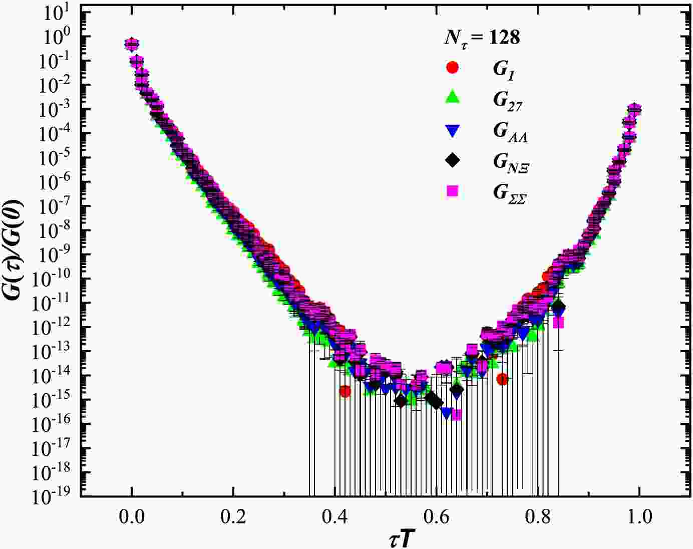
$ H_1 $ ,$ H_{27} $ ,$ H_{\Lambda\Lambda} $ ,$ H_{N\Xi} $ , and$ H_{\Sigma\Sigma} $ on the$ N_\tau=128 $ lattice are shown in Fig. 1. For completeness, the correlators on the other lattices are plotted in Fig. B1 in Appendix B. Some correlator data points on the$ N_\tau=128 $ lattice are negative and therefore are not shown because the vertical axis uses a logarithmic scale. Figure 1 and the figures in Appendix B show that the correlators of all five channels exhibit similar behavior on the same lattice. At some points, the error bars appear unusual because the errors are comparable to the correlator values themselves and the vertical axis is rescaled.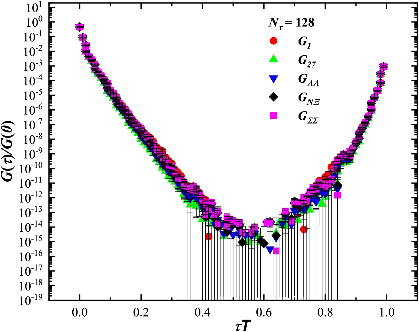
Figure 1. (color online) Euclidean correlators
$ G(\tau)/G(0) $ for$ H_1 $ ,$ H_{27} $ ,$ H_{\Lambda\Lambda} $ ,$ H_{N\Xi} $ , and$ H_{\Sigma\Sigma} $ as functions of$ \tau T $ on the$ N_\tau = 128 $ lattice, corresponding to the lowest temperature,$ T/T_c =0.24 $ . The correlators at some points are not shown because they have negative values. The vertical axis is logarithmically rescaled.To extract the ground-state energy, we employ an extrapolation method. Given the correlation functions, we obtain the mass by fitting the exponential ansatz:
$ \begin{array}{l} G(\tau) = A_+ {\rm e}^{-m_+\tau} + A_- {\rm e}^{-m_-(1/T-\tau)}, \end{array} $
(11) where
$ m_{+} $ is the mass of the particle of interest, and τ lies in the interval$ 0 \leq \tau \lt 1/T $ on a lattice at finite temperature T. Because excited states contribute more strongly at early Euclidean times [52], we first fit Eq. (11) to the correlator while excluding different early time slices, thereby obtaining a series of mass values. Specifically, we fit Eq. (11) to the correlator over the time interval$ [\tau_1, \tau_2] $ , where$ \tau_2 $ is fixed to the full temporal extent and$ \tau_1 $ takes several values, e.g.,$ \tau_1 = 0, 1, 2, 3, \dots $ . This procedure yields a series of mass values, each corresponding to a different fit range.After obtaining the series of mass values as a function of
$ 1/\tau_1 $ , we assume that they vary linearly with$ 1/\tau_1 $ and fit the following expression:$ \begin{array}{l} a_\tau m = A + B \dfrac{1}{\tau_1}. \end{array} $
(12) From this fit, we extrapolate the series of masses to
$ \tau_1 \to \infty $ .Our procedure consists of two fitting steps. In the first step, we fit the correlators using Eq. (11), which we refer to as the exponential fit. In the second step, we fit the series of mass values using Eq. (12), which we refer to as the linear fit.
We illustrate the extrapolation method used to extract the ground-state energy of
$ H_1 $ on the$ N_\tau = 128 $ lattice in detail. To control the uncertainties, all correlators are grouped using the bootstrap method.For each group of correlators, the mean value
$ G(\tau) $ is calculated. For every$ \tau_1 \in [0, 50] $ , we fit Eq. (11) to$ G(\tau) $ over the interval$ [\tau_1, \tau_2] $ with$ \tau_2 = 127 $ , obtaining the series of mass values shown in Fig. 2. The horizontal axis indicates the number of early time slices excluded from the exponential fit. As shown in Fig. 2, the extracted$ a_\tau m $ values are larger when fewer early time slices are excluded. However, suppressing too many early time slices leads to smaller$ a_\tau m $ values. In the intermediate region, applying a linear fit to the mass values as a function of$ 1/\tau_1 $ using Eq. (12) allows extrapolation to the limit$ \tau_1 \to \infty $ . Figure 3 also shows that, when$ \tau_1 $ is large, the$ a_\tau m $ values deviate significantly from the fitting curve. The resulting mass is taken as the ground-state energy of$ H_1 $ on the$ N_\tau = 128 $ lattice. This extrapolation procedure is illustrated in Fig. 3.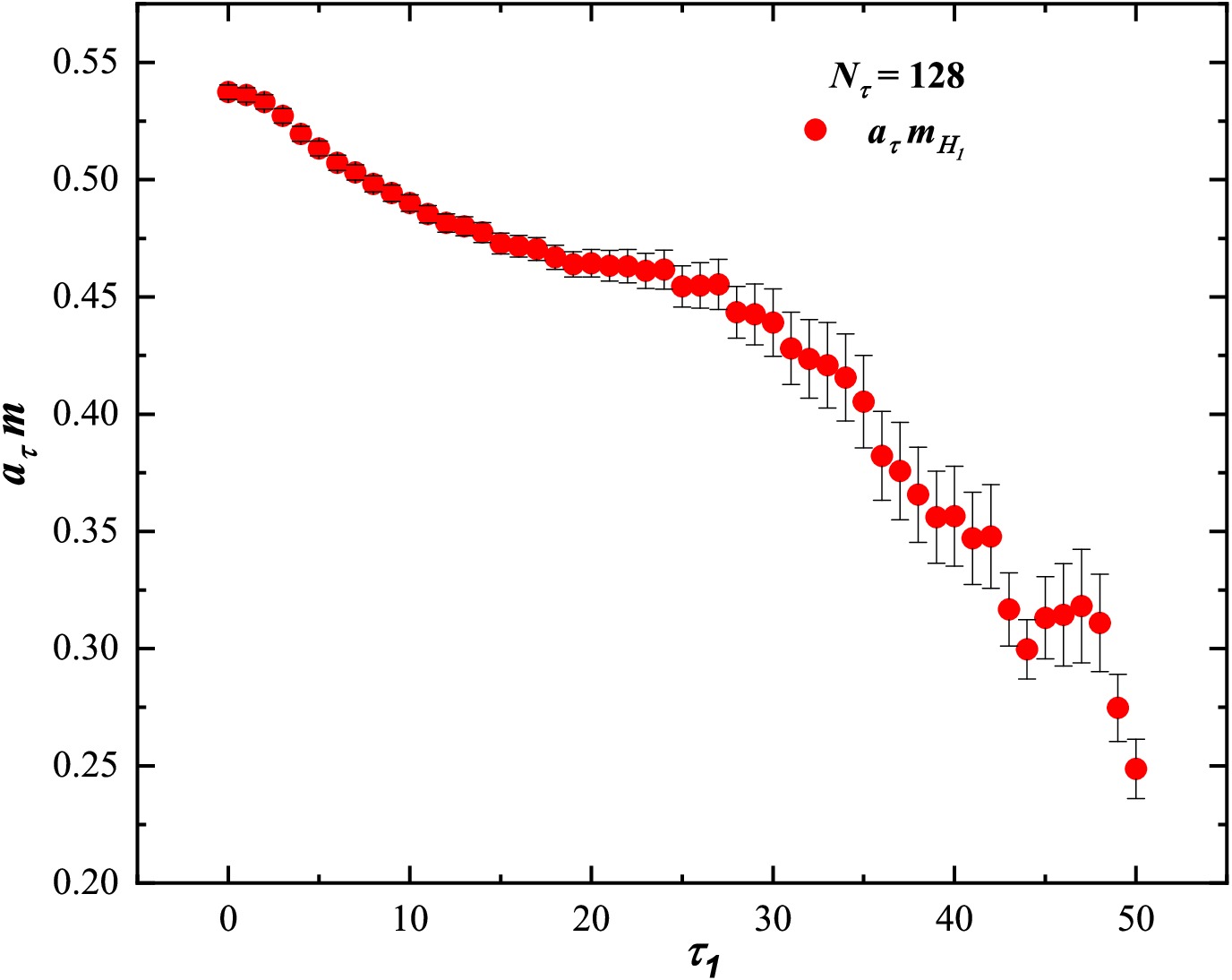
Figure 2. (color online) The
$ a_\tau m $ values for$ H_1 $ , obtained by fitting Eq. (11), are plotted as functions of the lower fit bound$ \tau_1 $ of the interval$ [\tau_1, \tau_2] $ , with the upper bound$ \tau_2 $ fixed at 127 on the$ N_\tau = 128 $ lattice.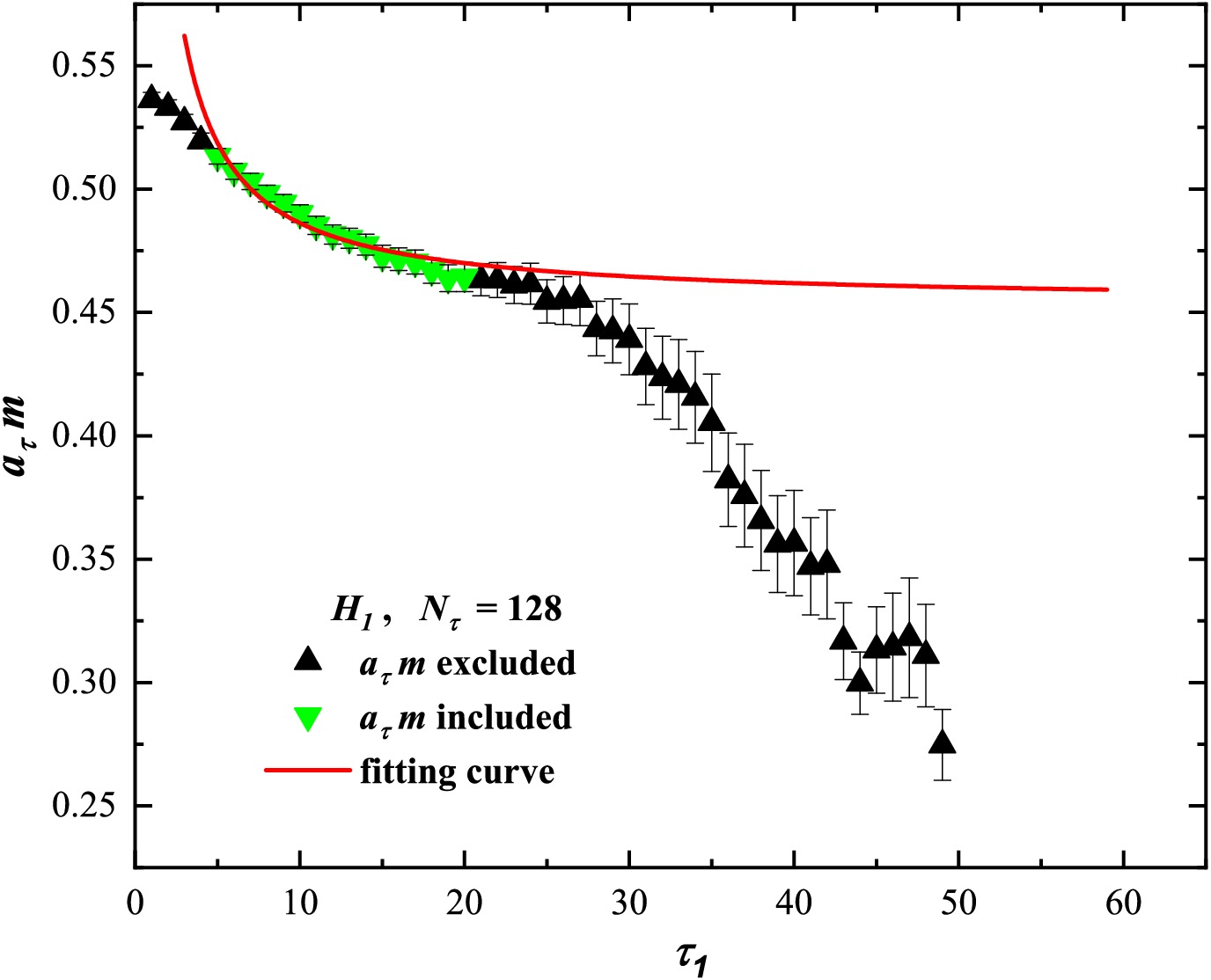
Figure 3. (color online) Linear extrapolation of the mass values for
$ H_1 $ on the$ N_\tau=128 $ lattice. The data points indicated by upward triangles are excluded from the extrapolation procedure, whereas the data points represented by downward triangles are included. The horizontal axis represents the lower fit bound$ \tau_1 $ of the interval$ [\tau_1, \tau_2] $ .For comparison, the effective mass of
$ H_1 $ on the$ N_\tau = 128 $ lattice is also computed using the following expression$ \begin{array}{l} a_\tau m_{\rm eff} = - \ln \dfrac{G(\tau+1)}{G(\tau)}. \end{array} $
(13) The result is presented in Fig. 4, from which 0.457 can be identified as the plateau value.
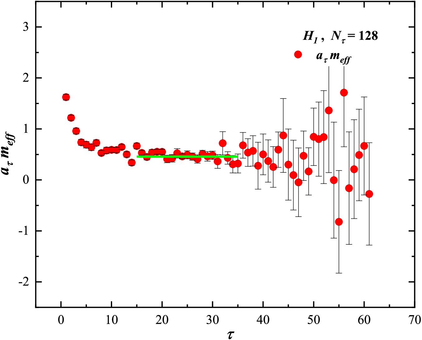
Figure 4. (color online) Effective mass of
$ H_1 $ on the$ N_\tau = 128 $ lattice. The green line denotes the plateau value of 0.457.The error estimation procedure requires explanation. For each group of correlators, exponential fitting is used to obtain a series of mass values. The errors from these exponential fits are used as weights in the subsequent linear fit to Eq. (12). The intercept of this linear fit gives the extrapolated value in the limit
$ \tau_1 \to \infty $ , and the error of the linear fit is taken as the systematic error for that group. After all bootstrap groups are processed, the overall systematic error is taken as the mean of the systematic errors from all groups. The statistical error is computed using the standard bootstrap method.The method described above is employed to compute the ground-state energy of
$ H_1 $ on the other lattices. The results are presented in Figs. 5−10. Figures 5, 7, and 9 show that, as the lattice size decreases from$ N_\tau = 48 $ to$ N_\tau = 16 $ , the plateau becomes increasingly difficult to identify from the effective mass plots. In Figs. 6, 8, and 10, the$ a_\tau m $ value at$ \tau_1 = 0 $ is not shown and is excluded from the linear fitting procedure. These figures also show that, at low temperatures, some early-time-slice$ a_\tau m $ values are excluded from the linear fits, whereas at high temperatures, suppressing early time slices leads to very small extrapolated values for$ H_1 $ .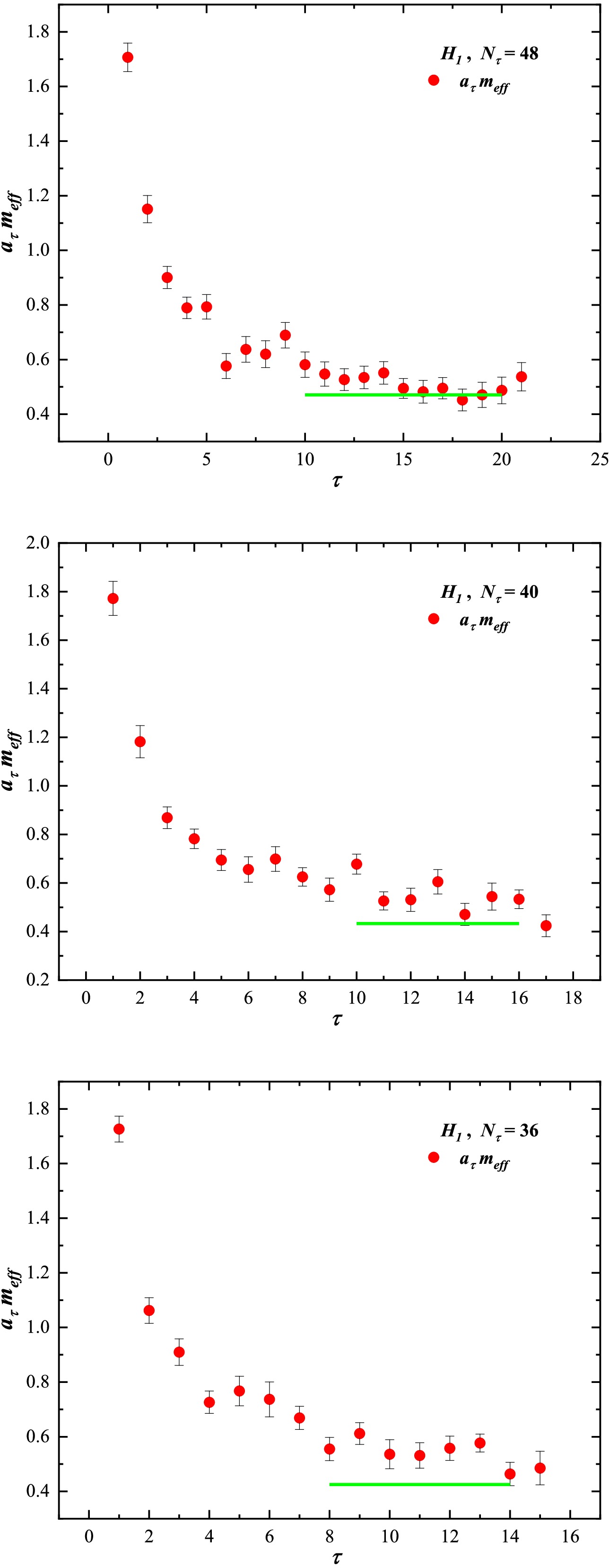
Figure 5. (color online) Effective mass of
$ H_1 $ on the$ N_\tau = $ 48, 40, 36 lattices. The green line represents the extrapolated mass value from Table 3.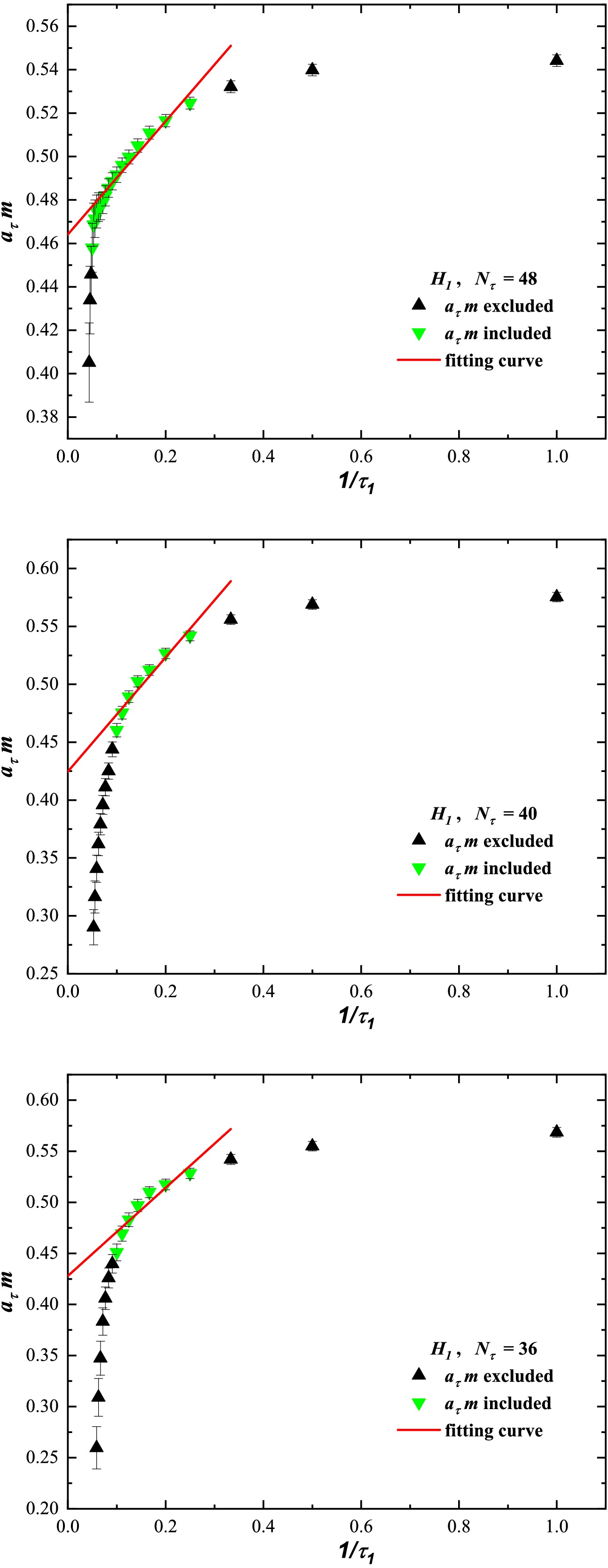
Figure 6. (color online) Linear fit of
$ a_\tau m $ versus$ 1/\tau_1 $ for one bootstrap group of$ H_1 $ correlators on the$ N_\tau = 48 $ ,$ 40 $ , and$ 36 $ lattices. The$ a_\tau m $ value at$ \tau_1 = 0 $ is not shown.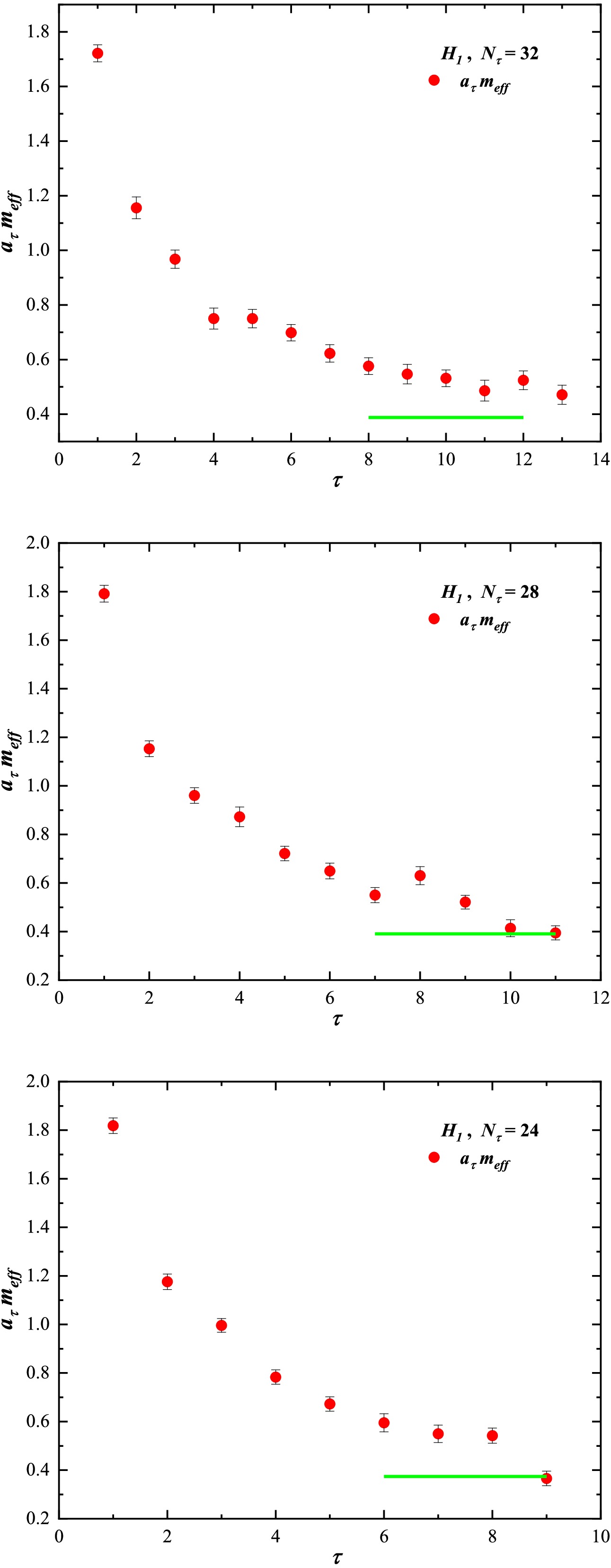
Figure 7. (color online) Effective mass of
$ H_1 $ on$ N_\tau = 32, 28, 24 $ lattices. The green line represents the extrapolated mass value from Table 3.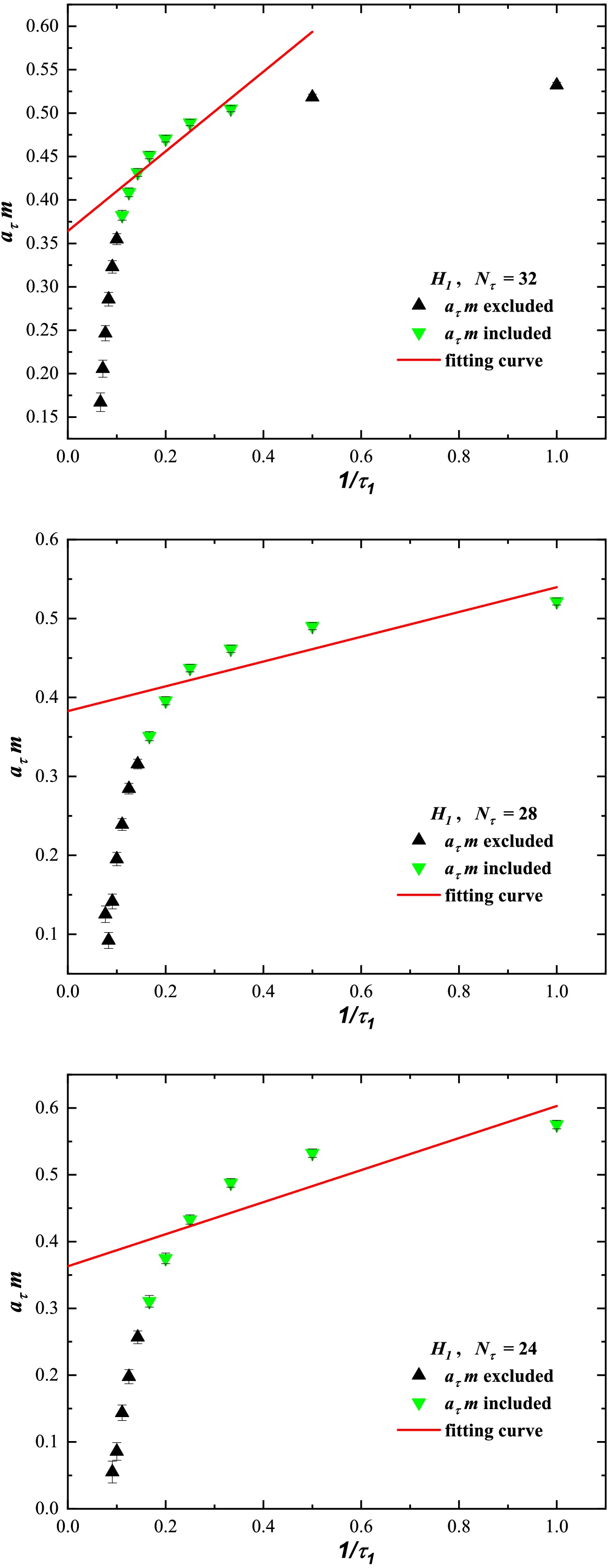
Figure 8. (color online) Linear fit of
$ a_\tau m $ versus$ 1/\tau_1 $ for one bootstrap group of$ H_1 $ correlators on the$ N_\tau = 32 $ ,$ 28 $ , and$ 24 $ lattices. The$ a_\tau m $ value at$ \tau_1 = 0 $ is not shown.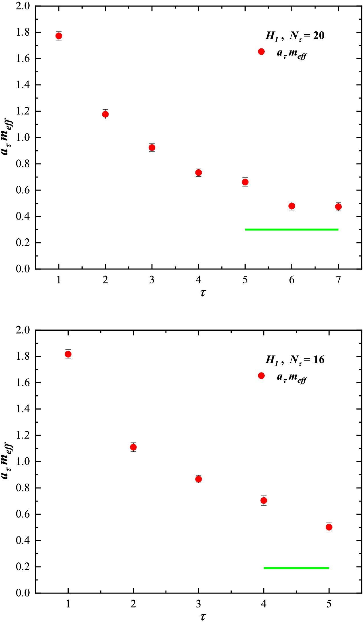
Figure 9. (color online) Effective mass of
$ H_1 $ on the$ N_\tau = 20, 16 $ lattices. The green line represents the extrapolated mass value from Table 3.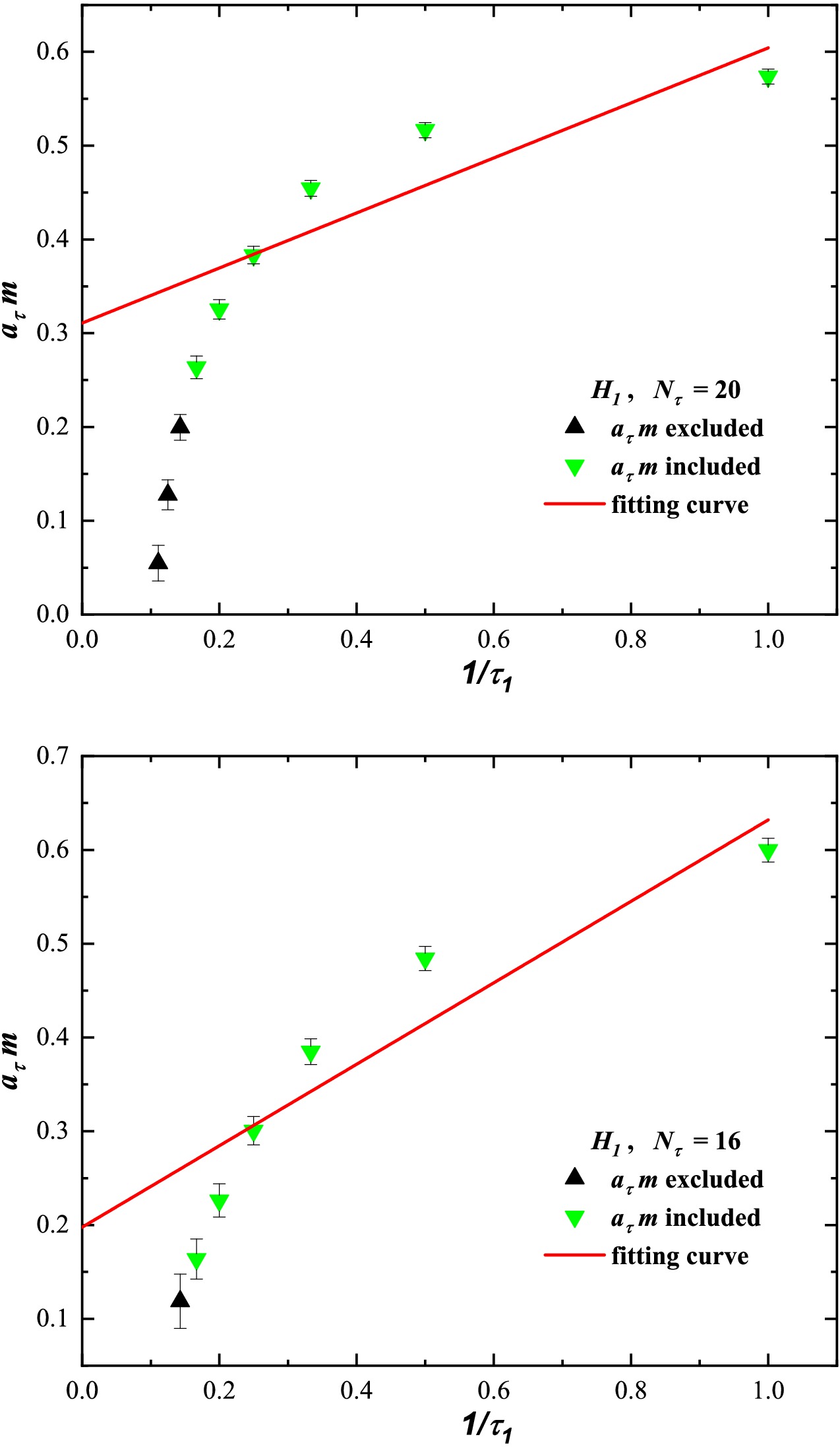
Figure 10. (color online) Linear fit of
$ a_\tau m $ versus$ 1/\tau_1 $ for one bootstrap group of$ H_1 $ correlators on the$ N_\tau = 20 $ , and$ 16 $ lattices. The$ a_\tau m $ value at$ \tau_1 = 0 $ is not shown.For the
$ H_{27} $ and$ H_{N\Xi} $ channels, the effective mass and linear fitting plots are shown in Figs. C1−C6 and Figs. C7−C12, respectively, in Appendix C. For the other channels, the effective mass and linear fits exhibit similar behavior, and the corresponding plots are omitted for brevity.We now turn to the results for all channels. The ground-state masses for
$ H_1 $ ,$ H_{27} $ ,$ H_{\Lambda\Lambda} $ ,$ H_{N\Xi} $ , and$ H_{\Sigma\Sigma} $ are listed in Table 3. From Table 3, we observe that among the five H-dibaryon channels, the mass of the 27-plet channel is the largest, whereas the mass of the$ \Sigma \Sigma $ channel is the lightest across the temperatures considered. We also plot these masses as functions of temperature in Fig. 11, which shows that they decrease with increasing temperature.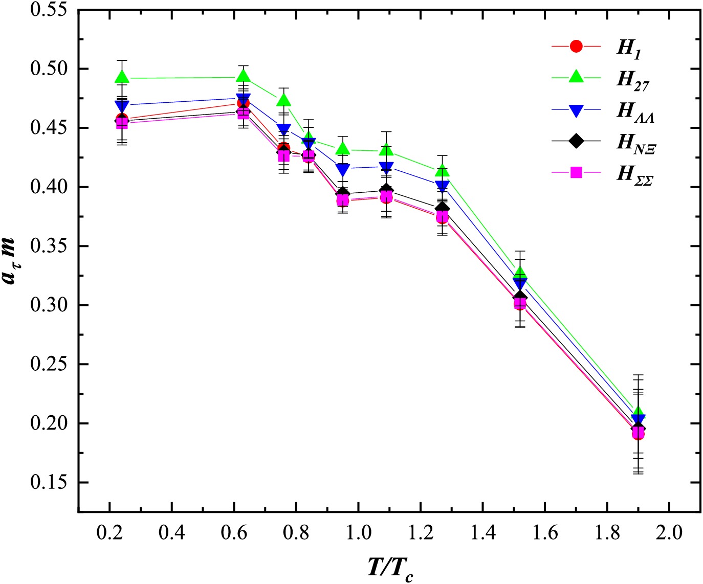
Figure 11. (color online) Mass values of
$ H_1 $ ,$ H_{27} $ ,$ H_{\Lambda\Lambda} $ ,$ H_{N\Xi} $ , and$ H_{\Sigma\Sigma} $ at nine temperatures.The fit quality of the exponential and linear fits requires further discussion. We use
$ \chi^2 $ to denote$ \chi^2 /{\rm d.o.f.} $ . The values of$ \chi^2 $ are collected in Tables 4 and 5. For the exponential fits, different levels of early-time-slice suppression yield different values of$ \chi^2 $ . Therefore, Table 4 shows only one value of$ \chi^2 $ for the exponential fit for each H-dibaryon channel, corresponding to a specific choice of$ \tau_1 $ . For the linear fit, the values of$ \chi^2 $ are large for lattices ranging from$ N_\tau = 32 $ down to$ N_\tau = 16 $ . If the first two or three$ a_\tau m $ values are excluded from the linear fit at high temperatures, the$ \chi^2 $ value can be reduced.$ N_\tau$ $H_1$ $H_{27}$ $H_{\Lambda\Lambda}$ $H_{N\Xi}$ $H_{\Sigma\Sigma}$ $\chi^2$ fit range $\chi^2$ fit range $\chi^2$ fit range $\chi^2$ fit range $\chi^2$ fit range 128 2.33 [18, 127] 2.33 [18, 127] 2.90 [18, 127] 2.43 [18, 127] 2.40 [18, 127] 48 6.93 [21, 47] 10.02 [21, 47] 10.10 [21, 47] 8.00 [21, 47] 7.27 [21, 47] 40 4.93 [12, 39] 7.81 [12, 39] 6.83 [12, 39] 5.42 [12, 39] 5.00 [12, 39] 36 10.85 [10, 35] 15.73 [10, 35] 14.15 [10, 35] 11.75 [10, 35] 10.92 [10, 35] 32 20.05 [8, 31] 21.99 [8, 31] 22.00 [8, 31] 20.77 [8, 31] 20.16 [8, 31] 28 21.15 [8, 27] 22.94 [8, 27] 22.49 [8, 27] 21.58 [8, 27] 21.21 [8, 27] 24 12.61 [7, 23] 13.19 [7, 23] 13.06 [7, 23] 12.77 [7, 23] 12.63 [7, 23] 20 16.37 [5, 19] 17.21 [5, 19] 17.01 [5, 19] 16.59 [5, 19] 16.40 [5, 19] 16 6.59 [4, 15] 6.48 [4, 15] 6.40 [4, 15] 6.24 [4, 15] 6.17 [4, 15] Table 4.
$\chi^2$ values obtained from exponential fits for one bootstrap group. On each lattice, varying$\tau_1$ produces a set of fit ranges$[\tau_1, \tau_2] $ with$\tau_2$ equal to the full temporal extent of the corresponding lattice. Each fit range yields a fitted mass$a_\tau m$ and an associated$\chi^2$ . Only the result for a single representative fit range is shown for each channel on each lattice.$ N_\tau$ $H_1$ $H_{27}$ $H_{\Lambda\Lambda}$ $H_{N\Xi}$ $H_{\Sigma\Sigma}$ $\chi^2$ fit range $\chi^2$ fit range $\chi^2$ fit range $\chi^2$ fit range $\chi^2$ fit range 128 0.9 [5, 20] 1.0 [5, 16] 1.5 [5, 18] 1.0 [5, 17] 1.0 [5, 18] 48 0.9 [4, 20] 0.9 [5, 14] 1.0 [5, 16] 1.0 [4, 14] 1.0 [4, 20] 40 2.6 [4, 10] 2.6 [4, 10] 2.9 [4, 10] 2.7 [4, 10] 2.6 [4, 10] 36 2.9 [4, 10] 5.4 [4, 10] 4.2 [4, 10] 3.3 [4, 10] 2.9 [4, 10] 32 16.4 [3, 9] 36.8 [2, 9] 36.4 [2, 9] 34.4 [2, 9] 16.5 [3, 9] 28 54.1 [1, 6] 65.9 [1, 6] 62.2 [1, 6] 56.4 [1, 6] 54.4 [1, 6] 24 66.1 [1, 6] 67.3 [1, 6] 67.5 [1, 6] 66.9 [1, 6] 66.2 [1, 6] 20 44.9 [1, 6] 46.8 [1, 6] 46.4 [1, 6] 45.4 [1, 6] 44.9 [1, 6] 16 20.2 [1, 6] 21.6 [1, 6] 21.3 [1, 6] 20.7 [1, 6] 20.4 [1, 6] Table 5.
$\chi^2$ values obtained from linear fits to the series of$a_\tau m$ values determined by fitting Eq. (11) for one bootstrap group.The mass values for
$ H_1 $ are slightly different from those in Ref. [53]. This is because, in Ref. [53], the correlator of each configuration is rescaled with respect to its own first time-slice value. In contrast, in this paper, the correlators of all configurations are rescaled with respect to the first time-slice value of the first configuration.We also calculate the spectral density
$ \bar\rho_L(E_\star) $ of the correlation functions of$ H_1 $ ,$ H_{27} $ ,$ H_{\Lambda\Lambda} $ ,$ H_{N\Xi} $ , and$ H_{\Sigma\Sigma} $ using the public computer program [64]. In Ref. [53], it was pointed out that, among the σ values$ \sigma=0.02, \, 0.04,\, 0.06,\, 0.08 $ ,$ \sigma =0.02 $ is the most suitable for spectral density extraction from correlators. At low temperatures, a smaller σ value reveals a rich peak structure in the small-$ E_\star $ region of the spectral density. At intermediate temperatures, a smaller σ value can make the peak structure in the small-$ E_\star $ region of the spectral density more pronounced. At high temperatures, different σ values have little impact on the computation of the spectral density. Therefore, we present only the spectral density results for$ \sigma =0.02 $ in Fig. 12 for all five channels.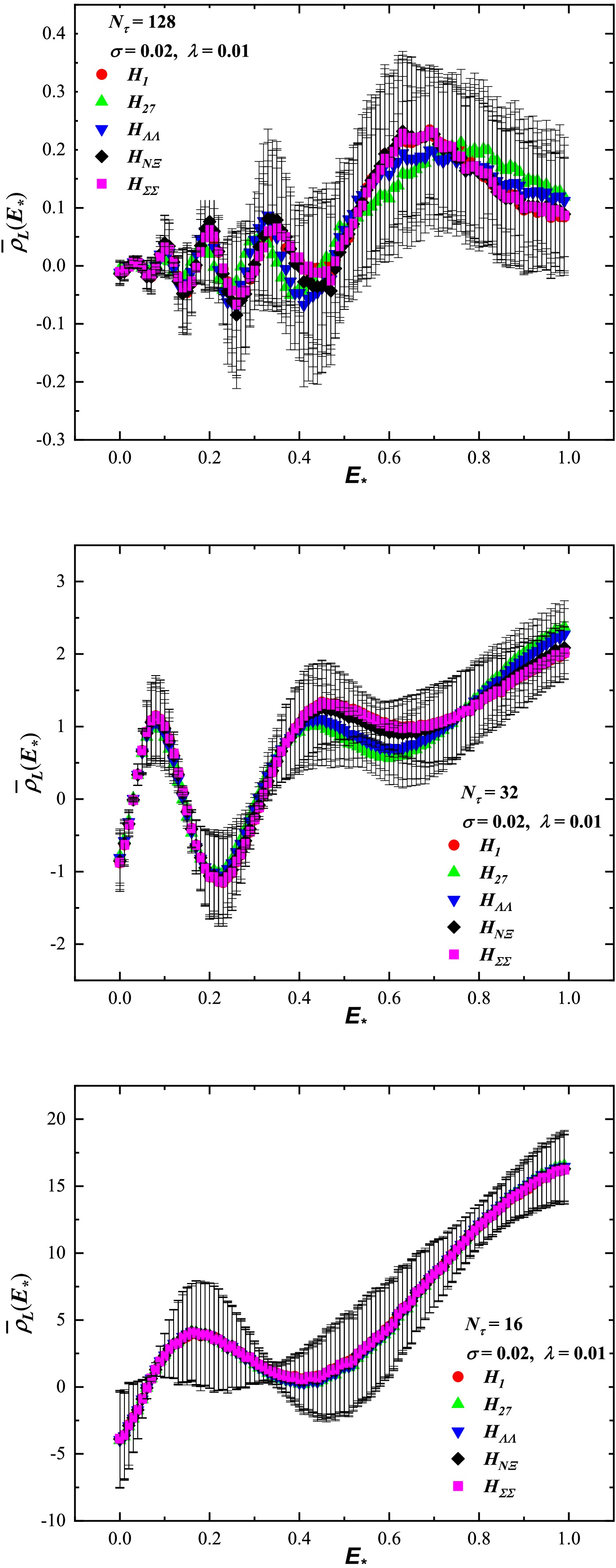
Figure 12. (color online) Spectral densities
$ \bar\rho_L(E_\star) $ for the$ H_1 $ ,$ H_{27} $ ,$ H_{\Lambda\Lambda} $ ,$ H_{N\Xi}, $ and$ H_{\Sigma\Sigma} $ channels at three temperatures. The upper, middle, and lower panels correspond to$ T/T_c = $ 0.24, 0.95, and$ 1.90 $ , respectively.Figure 12 presents the spectral densities
$ \bar\rho_L(E_\star) $ of$ H_1 $ ,$ H_{27} $ ,$ H_{\Lambda\Lambda} $ ,$ H_{N\Xi} $ , and$ H_{\Sigma\Sigma} $ at three temperatures. The upper, middle, and lower panels correspond to the$ N_\tau=128, \ 32, $ and$ 16 $ lattices, with$ T/T_c=0.24, \ 0.95, $ and$ 1.90 $ , respectively.As shown in Fig. 12, the reconstructed spectral densities of the five H-dibaryon channels exhibit similar qualitative structures at the three representative temperatures. At the lowest temperature, the spectral densities exhibit several peak-like structures. As the temperature increases to the intermediate region, these structures evolve into a two-peak pattern. At the highest temperature, the spectral distribution becomes further smoothed, and only one broad peak remains visible in the lower panel of Fig. 12.
At the lowest temperature,
$T/T_c=0.24$ , the masses extracted from the correlation function fits are approximately$a_\tau m\simeq0.45$ for the five channels, as listed in Table 3. These values are close to, but do not coincide exactly with, the main peak region around$E_\star\simeq0.35$ in the reconstructed spectral densities. In addition, the effective mass behavior shown in Fig. 4 gives a mass of about$a_\tau m\simeq0.45$ , whereas the corresponding spectral peak appears at a somewhat lower$E_\star$ . This discrepancy suggests that, in our simulations, the spectral density results should be interpreted with caution, although the reconstructed spectral densities can provide useful complementary information on the distribution and temperature dependence of the correlation functions.All of our results are obtained using an exponential ansatz for the correlator fits. In Ref. [65], the glueball correlators were fitted using a Breit-Wigner ansatz, which is given by the following expression (see Eq. (22) in Ref. [65]):
$ \begin{aligned}[b] G(\tau) =\;& A \Bigg[ \text{Re} \left( \dfrac{\cosh\left( (m + i\Gamma)\left(\dfrac{1}{2T} - \tau \right)\right)}{\sinh\left(\dfrac{m + i\Gamma}{2T}\right)} \right) \\& + 2 m T \sum_{n=1}^{\infty} \cos(2\pi n T \tau ) \\& \times \left\{ \dfrac{1}{(2\pi n T + \Gamma)^2 + m^2} - (n \to -n) \right\} \Bigg], \end{aligned} $
(14) where Γ denotes the resonance width.
We compare the extracted masses of the H-dibaryon in the
$ H_1 $ channel for different time-slice suppression parameters$ \tau_1 $ , using both the exponential and Breit-Wigner ansätze. The results on the$ N_\tau = 128 $ and$ N_\tau = 16 $ lattices are presented in Figs. 13 and 14, respectively.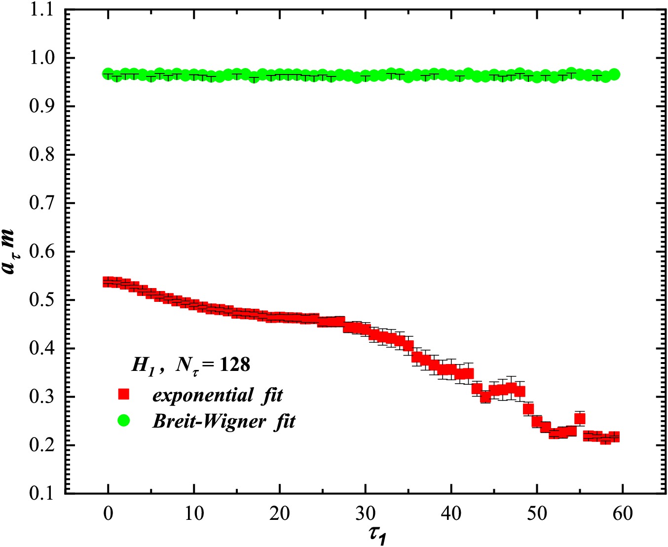
Figure 13. (color online) Comparison of the
$ a_\tau m $ values for$ H_1 $ extracted using the exponential and Breit-Wigner ansatzes, plotted as a function of the lower fit bound$ \tau_1 $ of the interval$ [\tau_1, \tau_2] $ , with$ \tau_2 $ fixed at 127 on the$ N_\tau = 128 $ lattice.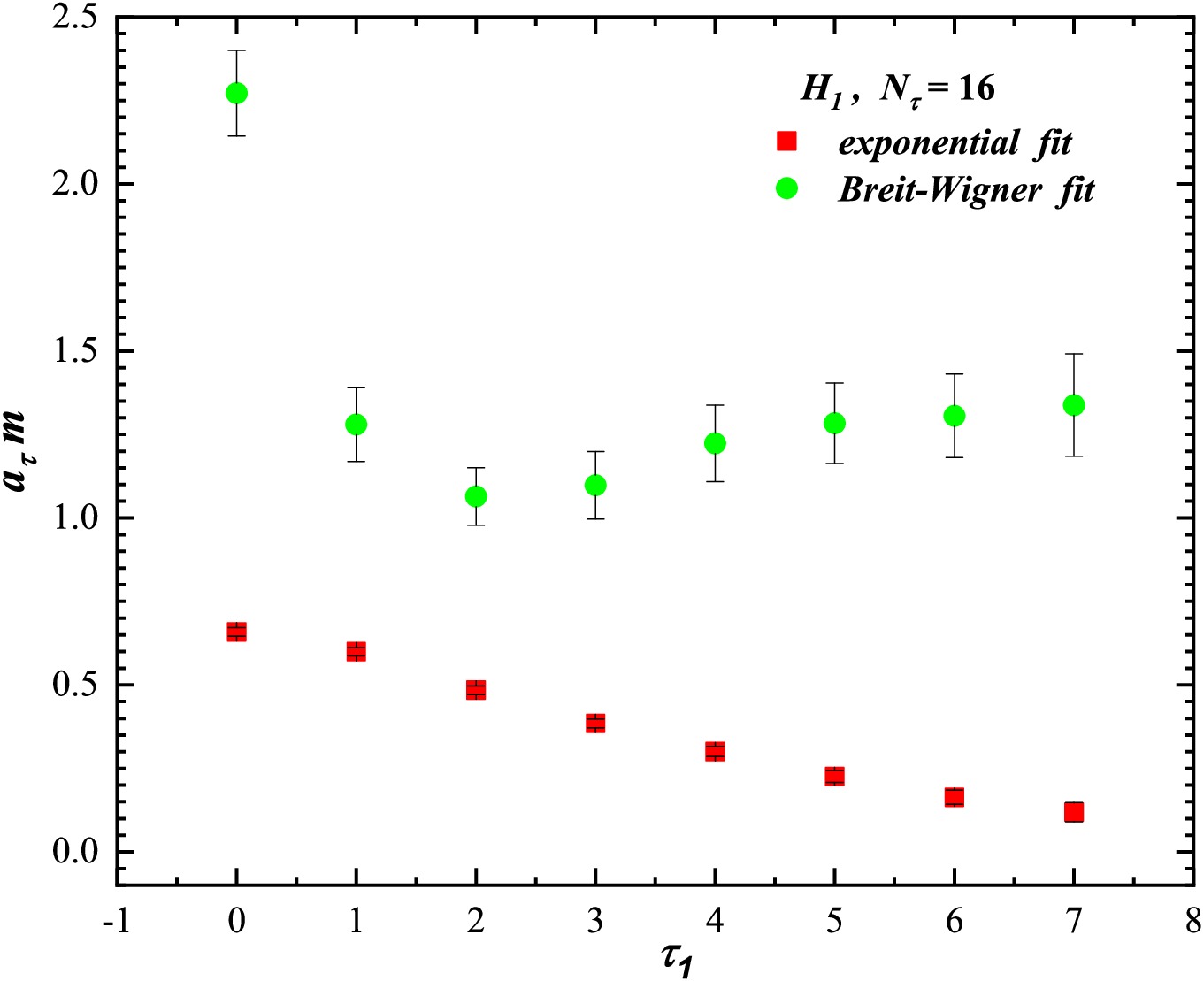
Figure 14. (color online) Comparison of the
$ a_\tau m $ values for$ H_1 $ extracted using the exponential and Breit-Wigner ansätze, plotted against the lower bound$ \tau_1 $ of the fit interval$ [\tau_1, \tau_2] $ , with$ \tau_2 $ fixed at 15 on the$ N_\tau = 16 $ lattice.As shown in Figs. 13 and 14, the
$ a_\tau m $ values obtained from the Breit-Wigner ansatz are significantly larger than those obtained from the exponential ansatz for$ H_1 $ on both the$ N_\tau = 128 $ and$ N_\tau = 16 $ lattices. Moreover, the$ a_\tau m $ values from the Breit-Wigner ansatz remain nearly constant on the$ N_\tau = 128 $ lattice, whereas they exhibit notable variation on the$ N_\tau = 16 $ lattice.For brevity, we do not show the remaining figures for other lattices and channels. Our simulation results indicate that, below the transition temperature, the
$ a_\tau m $ values extracted from the Breit-Wigner ansatz remain nearly constant with respect to$ \tau_1 $ , whereas above the transition temperature, their variation becomes increasingly significant.We have also examined the temperature dependence of the width Γ. We find that, as the temperature increases, Γ grows from the order of
$ 10^{-8} $ on the$ N_\tau = 128 $ lattice to a magnitude comparable to$ a_\tau m $ itself on the$ N_\tau = 16 $ lattice. -
The computational details are the same as those in Refs. [46, 53]. To make this paper self-contained, we briefly summarize them here. The simulations are carried out on
$ N_f=2+1 $ Generation 2 (Gen2) FASTSUM ensembles [46], with the lowest-temperature ensembles provided by the HadSpec collaboration [58, 59]. The ensembles are generated using a Symanzik-improved gauge action and a tadpole-improved clover fermion action with stout-smeared links.The parameters in the lattice action are listed in Table 1. The
$ N_f=2+1 $ Gen2 ensembles correspond to a physical strange quark mass and a bare light quark mass of$ a_\tau m_l = -0.0840 $ , yielding a pion mass of$ m_\pi=384(4)\, {\rm MeV} $ (see Table 2). The corresponding physical parameters, including the lattice spacing and the pion mass, are collected in Table 2. The lattice sizes and temperatures are given in Table 3.gauge coupling (fixed-scale approach) $ \beta = 1.5 $ tree-level coefficients $ c_0=5/3,\,c_1=-1/12 $ bare gauge, fermion anisotropy $ \gamma_g = 4.3 $ ,$ \gamma_f = 3.399 $ ratio of bare anisotropies $ \nu = \gamma_g / \gamma_f = 1.265 $ spatial tadpole (without, with smeared links) $ u_s = 0.733566 $ ,$ \tilde{u}_s = 0.92674 $ temporal tadpole (without, with smeared links) $ u_\tau = 1 $ ,$ \tilde u_\tau = 1 $ spatial, temporal clover coefficient $ c_s = 1.5893 $ ,$ c_\tau = 0.90278 $ stout smearing for spatial links $ \rho = 0.14 $ , isotropic, 2 stepsbare light quark mass for Gen2 $ \hat m_{0, \rm light} = -0.0840 $ bare strange quark mass $ \hat m_{0, \rm strange} = -0.0743 $ light quark hopping parameter for Gen2 $ \kappa_{\rm light} = 0.2780 $ strange quark hopping parameter $ \kappa_{\rm strange} = 0.2765 $ Table 1. Parameters in the lattice action. This table was compiled from Ref. [46].
$ a_\tau $ /fm0.0350(2) $ a_\tau^{-1} $ /GeV5.63(4) $ \xi=a_s/a_\tau $ 3.444(6) $ a_s $ /fm0.1205(8) $ N_s $ 24 $ m_\pi $ /MeV384(4) $ m_\pi L $ 5.63 Table 2. Parameters, including the lattice spacing and pion mass, were collected from Ref. [46] for the Generation 2 ensemble.
$ N_s $ $ N_\tau $ $T {\rm /MeV}$ $ T/T_c $ $ N_{\rm cfg} $ $ a_\tau m_{H_1} $ $ a_\tau m_{H_{27}} $ $ a_\tau m_{H_{\Lambda\Lambda}} $ $ a_\tau m_{H_{N\Xi}} $ $ a_\tau m_{H_{\Sigma\Sigma}} $ 24 128 44 0.24 305 0.457 (17) (3) 0.492 (15) (3) 0.469 (17) (3) 0.456 (18) (3) 0.454 (18) (3) 32 48 117 0.63 601 0.471 (10) (4) 0.493 (10) (4) 0.475 (11) (4) 0.464 (12) (4) 0.462 (12) (3) 24 40 141 0.76 502 0.433 (14) (14) 0.472 (11) (15) 0.450 (13) (16) 0.429 (14) (15) 0.426 (15) (14) 24 36 156 0.84 501 0.425 (13) (15) 0.440 (16) (19) 0.438 (13) (17) 0.427 (13) (16) 0.426 (13) (15) 24 32 176 0.95 1000 0.388 (10) (17) 0.431 (11) (19) 0.416 (11) (19) 0.394 (11) (18) 0.389 (10) (17) 24 28 201 1.09 1001 0.391 (17) (15) 0.430 (16) (18) 0.417 (17) (17) 0.397 (18) (16) 0.392 (17) (15) 24 24 235 1.27 1002 0.374 (15) (34) 0.413 (14) (34) 0.401 (14) (34) 0.382 (15) (35) 0.375 (15) (34) 24 20 281 1.52 1000 0.30 (2) (5) 0.33 (2) (5) 0.32 (2) (5) 0.31 (2) (5) 0.30 (2) (5) 24 16 352 1.90 1000 0.19 (3) (4) 0.21 (3) (5) 0.20 (3) (5) 0.20 (3) (5) 0.19 (3) (5) Table 3. Spatial and temporal extent, temperature (in MeV), number of configurations, and masses of
$ H_1 $ ,$ H_{27} $ ,$ H_{\Lambda\Lambda} $ ,$ H_{N\Xi} $ , and$ H_{\Sigma\Sigma} $ . Estimates of the statistical and systematic errors are given in the first and second brackets, respectively. The ensembles at the lowest temperatures were provided by HadSpec [58, 59] (Gen2).The quark propagators are computed using a deflation-accelerated algorithm [60, 61]. When computing the propagator, the spatial links are stout smeared [62] using two smearing steps and a weight of
$ \rho = 0.14 $ . For the sources and sinks, we use Gaussian smearing [63]$ \begin{array}{l} \eta' = C\left(1+\kappa H\right)^n\eta, \end{array} $
(10) where H denotes the spatial hopping part of the Dirac operator, and C is an appropriate normalisation [52].
The correlators of
$ H_1 $ ,$ H_{27} $ ,$ H_{\Lambda\Lambda} $ ,$ H_{N\Xi} $ , and$ H_{\Sigma\Sigma} $ on the$ N_\tau=128 $ lattice are shown in Fig. 1. For completeness, the correlators on the other lattices are plotted in Fig. B1 in Appendix B. Some correlator data points on the$ N_\tau=128 $ lattice are negative and therefore are not shown because the vertical axis uses a logarithmic scale. Figure 1 and the figures in Appendix B show that the correlators of all five channels exhibit similar behavior on the same lattice. At some points, the error bars appear unusual because the errors are comparable to the correlator values themselves and the vertical axis is rescaled.
Figure 1. (color online) Euclidean correlators
$ G(\tau)/G(0) $ for$ H_1 $ ,$ H_{27} $ ,$ H_{\Lambda\Lambda} $ ,$ H_{N\Xi} $ , and$ H_{\Sigma\Sigma} $ as functions of$ \tau T $ on the$ N_\tau = 128 $ lattice, corresponding to the lowest temperature,$ T/T_c =0.24 $ . The correlators at some points are not shown because they have negative values. The vertical axis is logarithmically rescaled.To extract the ground-state energy, we employ an extrapolation method. Given the correlation functions, we obtain the mass by fitting the exponential ansatz:
$ \begin{array}{l} G(\tau) = A_+ {\rm e}^{-m_+\tau} + A_- {\rm e}^{-m_-(1/T-\tau)}, \end{array} $
(11) where
$ m_{+} $ is the mass of the particle of interest, and τ lies in the interval$ 0 \leq \tau \lt 1/T $ on a lattice at finite temperature T. Because excited states contribute more strongly at early Euclidean times [52], we first fit Eq. (11) to the correlator while excluding different early time slices, thereby obtaining a series of mass values. Specifically, we fit Eq. (11) to the correlator over the time interval$ [\tau_1, \tau_2] $ , where$ \tau_2 $ is fixed to the full temporal extent and$ \tau_1 $ takes several values, e.g.,$ \tau_1 = 0, 1, 2, 3, \dots $ . This procedure yields a series of mass values, each corresponding to a different fit range.After obtaining the series of mass values as a function of
$ 1/\tau_1 $ , we assume that they vary linearly with$ 1/\tau_1 $ and fit the following expression:$ \begin{array}{l} a_\tau m = A + B \dfrac{1}{\tau_1}. \end{array} $
(12) From this fit, we extrapolate the series of masses to
$ \tau_1 \to \infty $ .Our procedure consists of two fitting steps. In the first step, we fit the correlators using Eq. (11), which we refer to as the exponential fit. In the second step, we fit the series of mass values using Eq. (12), which we refer to as the linear fit.
We illustrate the extrapolation method used to extract the ground-state energy of
$ H_1 $ on the$ N_\tau = 128 $ lattice in detail. To control the uncertainties, all correlators are grouped using the bootstrap method.For each group of correlators, the mean value
$ G(\tau) $ is calculated. For every$ \tau_1 \in [0, 50] $ , we fit Eq. (11) to$ G(\tau) $ over the interval$ [\tau_1, \tau_2] $ with$ \tau_2 = 127 $ , obtaining the series of mass values shown in Fig. 2. The horizontal axis indicates the number of early time slices excluded from the exponential fit. As shown in Fig. 2, the extracted$ a_\tau m $ values are larger when fewer early time slices are excluded. However, suppressing too many early time slices leads to smaller$ a_\tau m $ values. In the intermediate region, applying a linear fit to the mass values as a function of$ 1/\tau_1 $ using Eq. (12) allows extrapolation to the limit$ \tau_1 \to \infty $ . Figure 3 also shows that, when$ \tau_1 $ is large, the$ a_\tau m $ values deviate significantly from the fitting curve. The resulting mass is taken as the ground-state energy of$ H_1 $ on the$ N_\tau = 128 $ lattice. This extrapolation procedure is illustrated in Fig. 3.
Figure 2. (color online) The
$ a_\tau m $ values for$ H_1 $ , obtained by fitting Eq. (11), are plotted as functions of the lower fit bound$ \tau_1 $ of the interval$ [\tau_1, \tau_2] $ , with the upper bound$ \tau_2 $ fixed at 127 on the$ N_\tau = 128 $ lattice.
Figure 3. (color online) Linear extrapolation of the mass values for
$ H_1 $ on the$ N_\tau=128 $ lattice. The data points indicated by upward triangles are excluded from the extrapolation procedure, whereas the data points represented by downward triangles are included. The horizontal axis represents the lower fit bound$ \tau_1 $ of the interval$ [\tau_1, \tau_2] $ .For comparison, the effective mass of
$ H_1 $ on the$ N_\tau = 128 $ lattice is also computed using the following expression$ \begin{array}{l} a_\tau m_{\rm eff} = - \ln \dfrac{G(\tau+1)}{G(\tau)}. \end{array} $
(13) The result is presented in Fig. 4, from which 0.457 can be identified as the plateau value.
Figure 4. (color online) Effective mass of
$ H_1 $ on the$ N_\tau = 128 $ lattice. The green line denotes the plateau value of 0.457.The error estimation procedure requires explanation. For each group of correlators, exponential fitting is used to obtain a series of mass values. The errors from these exponential fits are used as weights in the subsequent linear fit to Eq. (12). The intercept of this linear fit gives the extrapolated value in the limit
$ \tau_1 \to \infty $ , and the error of the linear fit is taken as the systematic error for that group. After all bootstrap groups are processed, the overall systematic error is taken as the mean of the systematic errors from all groups. The statistical error is computed using the standard bootstrap method.The method described above is employed to compute the ground-state energy of
$ H_1 $ on the other lattices. The results are presented in Figs. 5−10. Figures 5, 7, and 9 show that, as the lattice size decreases from$ N_\tau = 48 $ to$ N_\tau = 16 $ , the plateau becomes increasingly difficult to identify from the effective mass plots. In Figs. 6, 8, and 10, the$ a_\tau m $ value at$ \tau_1 = 0 $ is not shown and is excluded from the linear fitting procedure. These figures also show that, at low temperatures, some early-time-slice$ a_\tau m $ values are excluded from the linear fits, whereas at high temperatures, suppressing early time slices leads to very small extrapolated values for$ H_1 $ .
Figure 5. (color online) Effective mass of
$ H_1 $ on the$ N_\tau = $ 48, 40, 36 lattices. The green line represents the extrapolated mass value from Table 3.
Figure 6. (color online) Linear fit of
$ a_\tau m $ versus$ 1/\tau_1 $ for one bootstrap group of$ H_1 $ correlators on the$ N_\tau = 48 $ ,$ 40 $ , and$ 36 $ lattices. The$ a_\tau m $ value at$ \tau_1 = 0 $ is not shown.
Figure 7. (color online) Effective mass of
$ H_1 $ on$ N_\tau = 32, 28, 24 $ lattices. The green line represents the extrapolated mass value from Table 3.
Figure 8. (color online) Linear fit of
$ a_\tau m $ versus$ 1/\tau_1 $ for one bootstrap group of$ H_1 $ correlators on the$ N_\tau = 32 $ ,$ 28 $ , and$ 24 $ lattices. The$ a_\tau m $ value at$ \tau_1 = 0 $ is not shown.
Figure 9. (color online) Effective mass of
$ H_1 $ on the$ N_\tau = 20, 16 $ lattices. The green line represents the extrapolated mass value from Table 3.
Figure 10. (color online) Linear fit of
$ a_\tau m $ versus$ 1/\tau_1 $ for one bootstrap group of$ H_1 $ correlators on the$ N_\tau = 20 $ , and$ 16 $ lattices. The$ a_\tau m $ value at$ \tau_1 = 0 $ is not shown.For the
$ H_{27} $ and$ H_{N\Xi} $ channels, the effective mass and linear fitting plots are shown in Figs. C1−C6 and Figs. C7−C12, respectively, in Appendix C. For the other channels, the effective mass and linear fits exhibit similar behavior, and the corresponding plots are omitted for brevity.We now turn to the results for all channels. The ground-state masses for
$ H_1 $ ,$ H_{27} $ ,$ H_{\Lambda\Lambda} $ ,$ H_{N\Xi} $ , and$ H_{\Sigma\Sigma} $ are listed in Table 3. From Table 3, we observe that among the five H-dibaryon channels, the mass of the 27-plet channel is the largest, whereas the mass of the$ \Sigma \Sigma $ channel is the lightest across the temperatures considered. We also plot these masses as functions of temperature in Fig. 11, which shows that they decrease with increasing temperature.
Figure 11. (color online) Mass values of
$ H_1 $ ,$ H_{27} $ ,$ H_{\Lambda\Lambda} $ ,$ H_{N\Xi} $ , and$ H_{\Sigma\Sigma} $ at nine temperatures.The fit quality of the exponential and linear fits requires further discussion. We use
$ \chi^2 $ to denote$ \chi^2 /{\rm d.o.f.} $ . The values of$ \chi^2 $ are collected in Tables 4 and 5. For the exponential fits, different levels of early-time-slice suppression yield different values of$ \chi^2 $ . Therefore, Table 4 shows only one value of$ \chi^2 $ for the exponential fit for each H-dibaryon channel, corresponding to a specific choice of$ \tau_1 $ . For the linear fit, the values of$ \chi^2 $ are large for lattices ranging from$ N_\tau = 32 $ down to$ N_\tau = 16 $ . If the first two or three$ a_\tau m $ values are excluded from the linear fit at high temperatures, the$ \chi^2 $ value can be reduced.$ N_\tau$ $H_1$ $H_{27}$ $H_{\Lambda\Lambda}$ $H_{N\Xi}$ $H_{\Sigma\Sigma}$ $\chi^2$ fit range $\chi^2$ fit range $\chi^2$ fit range $\chi^2$ fit range $\chi^2$ fit range 128 2.33 [18, 127] 2.33 [18, 127] 2.90 [18, 127] 2.43 [18, 127] 2.40 [18, 127] 48 6.93 [21, 47] 10.02 [21, 47] 10.10 [21, 47] 8.00 [21, 47] 7.27 [21, 47] 40 4.93 [12, 39] 7.81 [12, 39] 6.83 [12, 39] 5.42 [12, 39] 5.00 [12, 39] 36 10.85 [10, 35] 15.73 [10, 35] 14.15 [10, 35] 11.75 [10, 35] 10.92 [10, 35] 32 20.05 [8, 31] 21.99 [8, 31] 22.00 [8, 31] 20.77 [8, 31] 20.16 [8, 31] 28 21.15 [8, 27] 22.94 [8, 27] 22.49 [8, 27] 21.58 [8, 27] 21.21 [8, 27] 24 12.61 [7, 23] 13.19 [7, 23] 13.06 [7, 23] 12.77 [7, 23] 12.63 [7, 23] 20 16.37 [5, 19] 17.21 [5, 19] 17.01 [5, 19] 16.59 [5, 19] 16.40 [5, 19] 16 6.59 [4, 15] 6.48 [4, 15] 6.40 [4, 15] 6.24 [4, 15] 6.17 [4, 15] Table 4.
$\chi^2$ values obtained from exponential fits for one bootstrap group. On each lattice, varying$\tau_1$ produces a set of fit ranges$[\tau_1, \tau_2] $ with$\tau_2$ equal to the full temporal extent of the corresponding lattice. Each fit range yields a fitted mass$a_\tau m$ and an associated$\chi^2$ . Only the result for a single representative fit range is shown for each channel on each lattice.$ N_\tau$ $H_1$ $H_{27}$ $H_{\Lambda\Lambda}$ $H_{N\Xi}$ $H_{\Sigma\Sigma}$ $\chi^2$ fit range $\chi^2$ fit range $\chi^2$ fit range $\chi^2$ fit range $\chi^2$ fit range 128 0.9 [5, 20] 1.0 [5, 16] 1.5 [5, 18] 1.0 [5, 17] 1.0 [5, 18] 48 0.9 [4, 20] 0.9 [5, 14] 1.0 [5, 16] 1.0 [4, 14] 1.0 [4, 20] 40 2.6 [4, 10] 2.6 [4, 10] 2.9 [4, 10] 2.7 [4, 10] 2.6 [4, 10] 36 2.9 [4, 10] 5.4 [4, 10] 4.2 [4, 10] 3.3 [4, 10] 2.9 [4, 10] 32 16.4 [3, 9] 36.8 [2, 9] 36.4 [2, 9] 34.4 [2, 9] 16.5 [3, 9] 28 54.1 [1, 6] 65.9 [1, 6] 62.2 [1, 6] 56.4 [1, 6] 54.4 [1, 6] 24 66.1 [1, 6] 67.3 [1, 6] 67.5 [1, 6] 66.9 [1, 6] 66.2 [1, 6] 20 44.9 [1, 6] 46.8 [1, 6] 46.4 [1, 6] 45.4 [1, 6] 44.9 [1, 6] 16 20.2 [1, 6] 21.6 [1, 6] 21.3 [1, 6] 20.7 [1, 6] 20.4 [1, 6] Table 5.
$\chi^2$ values obtained from linear fits to the series of$a_\tau m$ values determined by fitting Eq. (11) for one bootstrap group.The mass values for
$ H_1 $ are slightly different from those in Ref. [53]. This is because, in Ref. [53], the correlator of each configuration is rescaled with respect to its own first time-slice value. In contrast, in this paper, the correlators of all configurations are rescaled with respect to the first time-slice value of the first configuration.We also calculate the spectral density
$ \bar\rho_L(E_\star) $ of the correlation functions of$ H_1 $ ,$ H_{27} $ ,$ H_{\Lambda\Lambda} $ ,$ H_{N\Xi} $ , and$ H_{\Sigma\Sigma} $ using the public computer program [64]. In Ref. [53], it was pointed out that, among the σ values$ \sigma=0.02, \, 0.04,\, 0.06,\, 0.08 $ ,$ \sigma =0.02 $ is the most suitable for spectral density extraction from correlators. At low temperatures, a smaller σ value reveals a rich peak structure in the small-$ E_\star $ region of the spectral density. At intermediate temperatures, a smaller σ value can make the peak structure in the small-$ E_\star $ region of the spectral density more pronounced. At high temperatures, different σ values have little impact on the computation of the spectral density. Therefore, we present only the spectral density results for$ \sigma =0.02 $ in Fig. 12 for all five channels.
Figure 12. (color online) Spectral densities
$ \bar\rho_L(E_\star) $ for the$ H_1 $ ,$ H_{27} $ ,$ H_{\Lambda\Lambda} $ ,$ H_{N\Xi}, $ and$ H_{\Sigma\Sigma} $ channels at three temperatures. The upper, middle, and lower panels correspond to$ T/T_c = $ 0.24, 0.95, and$ 1.90 $ , respectively.Figure 12 presents the spectral densities
$ \bar\rho_L(E_\star) $ of$ H_1 $ ,$ H_{27} $ ,$ H_{\Lambda\Lambda} $ ,$ H_{N\Xi} $ , and$ H_{\Sigma\Sigma} $ at three temperatures. The upper, middle, and lower panels correspond to the$ N_\tau=128, \ 32, $ and$ 16 $ lattices, with$ T/T_c=0.24, \ 0.95, $ and$ 1.90 $ , respectively.As shown in Fig. 12, the reconstructed spectral densities of the five H-dibaryon channels exhibit similar qualitative structures at the three representative temperatures. At the lowest temperature, the spectral densities exhibit several peak-like structures. As the temperature increases to the intermediate region, these structures evolve into a two-peak pattern. At the highest temperature, the spectral distribution becomes further smoothed, and only one broad peak remains visible in the lower panel of Fig. 12.
At the lowest temperature,
$T/T_c=0.24$ , the masses extracted from the correlation function fits are approximately$a_\tau m\simeq0.45$ for the five channels, as listed in Table 3. These values are close to, but do not coincide exactly with, the main peak region around$E_\star\simeq0.35$ in the reconstructed spectral densities. In addition, the effective mass behavior shown in Fig. 4 gives a mass of about$a_\tau m\simeq0.45$ , whereas the corresponding spectral peak appears at a somewhat lower$E_\star$ . This discrepancy suggests that, in our simulations, the spectral density results should be interpreted with caution, although the reconstructed spectral densities can provide useful complementary information on the distribution and temperature dependence of the correlation functions.All of our results are obtained using an exponential ansatz for the correlator fits. In Ref. [65], the glueball correlators were fitted using a Breit-Wigner ansatz, which is given by the following expression (see Eq. (22) in Ref. [65]):
$ \begin{aligned}[b] G(\tau) =\;& A \Bigg[ \text{Re} \left( \dfrac{\cosh\left( (m + i\Gamma)\left(\dfrac{1}{2T} - \tau \right)\right)}{\sinh\left(\dfrac{m + i\Gamma}{2T}\right)} \right) \\& + 2 m T \sum_{n=1}^{\infty} \cos(2\pi n T \tau ) \\& \times \left\{ \dfrac{1}{(2\pi n T + \Gamma)^2 + m^2} - (n \to -n) \right\} \Bigg], \end{aligned} $
(14) where Γ denotes the resonance width.
We compare the extracted masses of the H-dibaryon in the
$ H_1 $ channel for different time-slice suppression parameters$ \tau_1 $ , using both the exponential and Breit-Wigner ansätze. The results on the$ N_\tau = 128 $ and$ N_\tau = 16 $ lattices are presented in Figs. 13 and 14, respectively.
Figure 13. (color online) Comparison of the
$ a_\tau m $ values for$ H_1 $ extracted using the exponential and Breit-Wigner ansatzes, plotted as a function of the lower fit bound$ \tau_1 $ of the interval$ [\tau_1, \tau_2] $ , with$ \tau_2 $ fixed at 127 on the$ N_\tau = 128 $ lattice.
Figure 14. (color online) Comparison of the
$ a_\tau m $ values for$ H_1 $ extracted using the exponential and Breit-Wigner ansätze, plotted against the lower bound$ \tau_1 $ of the fit interval$ [\tau_1, \tau_2] $ , with$ \tau_2 $ fixed at 15 on the$ N_\tau = 16 $ lattice.As shown in Figs. 13 and 14, the
$ a_\tau m $ values obtained from the Breit-Wigner ansatz are significantly larger than those obtained from the exponential ansatz for$ H_1 $ on both the$ N_\tau = 128 $ and$ N_\tau = 16 $ lattices. Moreover, the$ a_\tau m $ values from the Breit-Wigner ansatz remain nearly constant on the$ N_\tau = 128 $ lattice, whereas they exhibit notable variation on the$ N_\tau = 16 $ lattice.For brevity, we do not show the remaining figures for other lattices and channels. Our simulation results indicate that, below the transition temperature, the
$ a_\tau m $ values extracted from the Breit-Wigner ansatz remain nearly constant with respect to$ \tau_1 $ , whereas above the transition temperature, their variation becomes increasingly significant.We have also examined the temperature dependence of the width Γ. We find that, as the temperature increases, Γ grows from the order of
$ 10^{-8} $ on the$ N_\tau = 128 $ lattice to a magnitude comparable to$ a_\tau m $ itself on the$ N_\tau = 16 $ lattice. -
We performed simulations to determine the masses of five channels of the conjectured H-dibaryon in
$ 2+1 $ flavor QCD with clover fermions at nine temperatures. The results are summarized in Table 3. The spectral density distributions of the correlation functions for these channels were computed to examine the mass spectrum obtained from the fitting procedure.In the simulations, the logarithmically rescaled correlators of the five channels differ only slightly, and their spectral densities exhibit nearly identical structures. However, using the extrapolation method described in Sec. III, the mass values of the five channels can be obtained, as presented in Table 3.
At the lowest temperature, the
$ a_\tau m $ value for$ H_{27} $ is$ 0.492(15)(3) $ , the largest among the five channels. The corresponding values for$ H_1 $ ,$ H_{\Lambda\Lambda} $ , and$ H_{\Sigma\Sigma} $ are$ 0.457(17)(3) $ ,$ 0.456(18)(3) $ , and$ 0.454(18)(3) $ , respectively, and differ only slightly. Using the Λ baryon mass from Table 3 in Ref. [53], together with the masses of the five channels from Table 3, we estimate the mass difference$ \Delta m \equiv m_H - 2m_\Lambda $ . The results are as follows:$ \begin{array}{l} \Delta m = m_{H_1} - 2m_\Lambda = -0.003(18)(3), \end{array} $
(15) $ \begin{array}{l} \Delta m = m_{H_{27}} - 2m_\Lambda = 0.032(16)(3), \end{array} $
(16) $ \begin{array}{l} \Delta m = m_{H_{\Lambda\Lambda}} - 2m_\Lambda = 0.009(17)(3), \end{array} $
(17) $ \begin{array}{l} \Delta m = m_{H_{N\Xi}} - 2m_\Lambda = -0.004(18)(3), \end{array} $
(18) $ \begin{array}{l} \Delta m = m_{H_{\Sigma\Sigma}} - 2m_\Lambda = -0.006(18)(3). \end{array} $
(19) The errors given in the first and second parentheses correspond to the statistical and systematic uncertainties, respectively. Each was evaluated using the error propagation formula, i.e.,
$ \sigma_{A-2B} = \sqrt{\sigma_A^2 + 4\sigma_B^2} $ , applied separately to each error component.Using the lattice spacing presented in Table 2, the results can be converted to physical units. All of our simulations were carried out at a single volume and at
$ m_\pi = 384(4)\, {\rm MeV} $ , which is far from the physical pion mass. The results of our current simulations show that, at$ m_\pi=384(4)\,{\rm MeV} $ ,$ \Delta m $ is positive for the$ H_{27} $ and$ H_{\Lambda\Lambda} $ channels. After conversion to physical units,$ \Delta m $ for the$ H_{27} $ channel is approximately$ 180 \,{\rm MeV} $ , indicating that the mass of the$ H_{27} $ channel is much heavier than$ 2m_\Lambda $ at$ m_\pi = 384(4) \, {\rm MeV} $ . In contrast, the masses of the$ H_{1}, H_{N\Xi} $ and$ H_{\Sigma\Sigma} $ channels are slightly lighter than$ 2m_\Lambda $ and are all of the same order of magnitude.Given the large
$ \chi^2 $ values in Tables 4 and 5, along with the linear-fit plots at high temperatures, the linearly extrapolated masses of the various H-dibaryon channels at high temperatures exhibit significant sensitivity to the choice of fit range. Consequently, these masses should be regarded as exploratory estimates rather than precise determinations, particularly in the high-temperature region.Similarly, the main conclusion of this work does not lie in the exact absolute values of the extracted masses, but rather in the comparative channel dependence under this ensemble setup. Specifically, the 27-plet channel tends to be the heaviest, while the
$ \Sigma\Sigma $ channel is among the lighter ones.Our simulations are limited to a single volume and a pion mass of
$ m_\pi = 384(4) \, {\rm MeV} $ . One main reason why our linear-fit results at high temperatures are sensitive to the fit range is that our lattice has a small temporal extent, which limits the available information. To draw stronger conclusions about$\Delta m$ and the possible binding of the H-dibaryon, significantly smaller quark masses and larger volumes are needed. However, performing lattice simulations at both high temperatures and large volumes is technically challenging, because a large temporal extent at high temperature requires a very fine lattice spacing. Further discussion of the H-dibaryon binding energy can be found in Ref. [53] and references therein.In our simulation, the change in temperature is represented by the change in
$ T/T_c $ .$ T_c $ is the pseudocritical temperature determined using the renormalized Polyakov loop and estimated to be$ T_c = 185(4)\, {\rm MeV} $ [46, 66]. -
We performed simulations to determine the masses of five channels of the conjectured H-dibaryon in
$ 2+1 $ flavor QCD with clover fermions at nine temperatures. The results are summarized in Table 3. The spectral density distributions of the correlation functions for these channels were computed to examine the mass spectrum obtained from the fitting procedure.In the simulations, the logarithmically rescaled correlators of the five channels differ only slightly, and their spectral densities exhibit nearly identical structures. However, using the extrapolation method described in Sec. III, the mass values of the five channels can be obtained, as presented in Table 3.
At the lowest temperature, the
$ a_\tau m $ value for$ H_{27} $ is$ 0.492(15)(3) $ , the largest among the five channels. The corresponding values for$ H_1 $ ,$ H_{\Lambda\Lambda} $ , and$ H_{\Sigma\Sigma} $ are$ 0.457(17)(3) $ ,$ 0.456(18)(3) $ , and$ 0.454(18)(3) $ , respectively, and differ only slightly. Using the Λ baryon mass from Table 3 in Ref. [53], together with the masses of the five channels from Table 3, we estimate the mass difference$ \Delta m \equiv m_H - 2m_\Lambda $ . The results are as follows:$ \begin{array}{l} \Delta m = m_{H_1} - 2m_\Lambda = -0.003(18)(3), \end{array} $
(15) $ \begin{array}{l} \Delta m = m_{H_{27}} - 2m_\Lambda = 0.032(16)(3), \end{array} $
(16) $ \begin{array}{l} \Delta m = m_{H_{\Lambda\Lambda}} - 2m_\Lambda = 0.009(17)(3), \end{array} $
(17) $ \begin{array}{l} \Delta m = m_{H_{N\Xi}} - 2m_\Lambda = -0.004(18)(3), \end{array} $
(18) $ \begin{array}{l} \Delta m = m_{H_{\Sigma\Sigma}} - 2m_\Lambda = -0.006(18)(3). \end{array} $
(19) The errors given in the first and second parentheses correspond to the statistical and systematic uncertainties, respectively. Each was evaluated using the error propagation formula, i.e.,
$ \sigma_{A-2B} = \sqrt{\sigma_A^2 + 4\sigma_B^2} $ , applied separately to each error component.Using the lattice spacing presented in Table 2, the results can be converted to physical units. All of our simulations were carried out at a single volume and at
$ m_\pi = 384(4)\, {\rm MeV} $ , which is far from the physical pion mass. The results of our current simulations show that, at$ m_\pi=384(4)\,{\rm MeV} $ ,$ \Delta m $ is positive for the$ H_{27} $ and$ H_{\Lambda\Lambda} $ channels. After conversion to physical units,$ \Delta m $ for the$ H_{27} $ channel is approximately$ 180 \,{\rm MeV} $ , indicating that the mass of the$ H_{27} $ channel is much heavier than$ 2m_\Lambda $ at$ m_\pi = 384(4) \, {\rm MeV} $ . In contrast, the masses of the$ H_{1}, H_{N\Xi} $ and$ H_{\Sigma\Sigma} $ channels are slightly lighter than$ 2m_\Lambda $ and are all of the same order of magnitude.Given the large
$ \chi^2 $ values in Tables 4 and 5, along with the linear-fit plots at high temperatures, the linearly extrapolated masses of the various H-dibaryon channels at high temperatures exhibit significant sensitivity to the choice of fit range. Consequently, these masses should be regarded as exploratory estimates rather than precise determinations, particularly in the high-temperature region.Similarly, the main conclusion of this work does not lie in the exact absolute values of the extracted masses, but rather in the comparative channel dependence under this ensemble setup. Specifically, the 27-plet channel tends to be the heaviest, while the
$ \Sigma\Sigma $ channel is among the lighter ones.Our simulations are limited to a single volume and a pion mass of
$ m_\pi = 384(4) \, {\rm MeV} $ . One main reason why our linear-fit results at high temperatures are sensitive to the fit range is that our lattice has a small temporal extent, which limits the available information. To draw stronger conclusions about$\Delta m$ and the possible binding of the H-dibaryon, significantly smaller quark masses and larger volumes are needed. However, performing lattice simulations at both high temperatures and large volumes is technically challenging, because a large temporal extent at high temperature requires a very fine lattice spacing. Further discussion of the H-dibaryon binding energy can be found in Ref. [53] and references therein.In our simulation, the change in temperature is represented by the change in
$ T/T_c $ .$ T_c $ is the pseudocritical temperature determined using the renormalized Polyakov loop and estimated to be$ T_c = 185(4)\, {\rm MeV} $ [46, 66]. -
We thank Gert Aarts, Simon Hands, Chris Allton, and Jonas Glesaaen for their valuable help. We modified the adapted versions of the OpenQCD code [67] and the MILC code [68] to carry out this simulation, and used the computer program [64] to calculate the spectral densities. The adapted version of the OpenQCD code is publicly available [69]. The simulations were carried out on
$ N_f=2+1 $ Generation 2 (Gen2) FASTSUM ensembles [46], with those at the lowest temperature provided by the HadSpec collaboration [58, 59]. The computations were performed on the high-performance computing platform of Jiangsu University. -
We thank Gert Aarts, Simon Hands, Chris Allton, and Jonas Glesaaen for their valuable help. We modified the adapted versions of the OpenQCD code [67] and the MILC code [68] to carry out this simulation, and used the computer program [64] to calculate the spectral densities. The adapted version of the OpenQCD code is publicly available [69]. The simulations were carried out on
$ N_f=2+1 $ Generation 2 (Gen2) FASTSUM ensembles [46], with those at the lowest temperature provided by the HadSpec collaboration [58, 59]. The computations were performed on the high-performance computing platform of Jiangsu University. -
The correlation function
$ G_1 $ for the$ H_1 $ channel can be found in Ref. [56]. The correlation functions$ G_{27} $ ,$ G_{\Lambda\Lambda} $ ,$ G_{N\Xi} $ , and$ G_{\Sigma\Sigma} $ for the$ H_{27} $ ,$ H_{\Lambda\Lambda} $ ,$ H_{N\Xi} $ , and$ H_{\Sigma\Sigma} $ channels, respectively, are given by the following expressions:$ \begin{aligned}[b] G_{27} =\;& \epsilon_{abc}\epsilon_{def}\epsilon_{ghi}\epsilon_{jkl} (C\gamma_{5}P_+)_{\beta\gamma} (C\gamma_{5}P_+)_{\epsilon\phi} (C\gamma_{5}P_+)_{\delta\alpha} (C\gamma_{5}P_+)_{\rho\sigma} (C\gamma_{5}P_+)_{\mu\nu} (C\gamma_{5}P_+)_{\lambda\tau}\\& \times \big\{ 9 \times ( S_{\alpha a,\tau j} S_{\delta d,\lambda g} - S_{\alpha a,\lambda g} S_{\delta d,\tau j} ) ( U_{\beta b,\nu k} U_{\epsilon e,\sigma h} - U_{\beta b,\sigma h} U_{\epsilon e,\nu k} ) ( D_{\gamma c,\mu l} D_{\phi f,\rho i} - D_{\gamma c,\rho i} D_{\phi f,\mu l} ) \\&+ 3 \times ( S_{\alpha a,\rho i} S_{\delta d,\lambda g} - S_{\alpha a,\lambda g} S_{\delta d,\rho i} ) ( U_{\beta b,\tau j} U_{\epsilon e,\mu l} - U_{\beta b,\mu l} U_{\epsilon e,\tau j} ) ( D_{\gamma c,\nu k} D_{\phi f,\sigma h} - D_{\gamma c,\sigma h} D_{\phi f,\nu k} ) \\&+ 3 \times ( S_{\alpha a,\rho i} S_{\delta d,\lambda g} - S_{\alpha a,\lambda g} S_{\delta d,\rho i} ) ( U_{\beta b,\nu k} U_{\epsilon e,\sigma h} - U_{\beta b,\sigma h} U_{\epsilon e,\nu k} ) ( D_{\gamma c,\tau j} D_{\phi f,\mu l} - D_{\gamma c,\mu l} D_{\phi f,\tau j} ) \\&+ 3 \times ( S_{\delta d,\lambda g} S_{\phi f,\tau j} - S_{\delta d,\tau j} S_{\phi f,\lambda g} ) ( U_{\alpha a,\nu k} U_{\gamma c,\sigma h} - U_{\alpha a,\sigma h} U_{\gamma c,\nu k} ) ( D_{\beta b,\mu l} D_{\epsilon e,\rho i} - D_{\beta b,\rho i} D_{\epsilon e,\mu l} ) \\&+ ( S_{\delta d,\lambda g} S_{\phi f,\rho i} - S_{\delta d,\rho i} S_{\phi f,\lambda g} ) ( U_{\alpha a,\tau j} U_{\gamma c,\mu l} - U_{\alpha a,\mu l} U_{\gamma c,\tau j} ) ( D_{\beta b,\nu k} D_{\epsilon e,\sigma h} - D_{\beta b,\sigma h} D_{\epsilon e,\nu k} ) \end{aligned} $
$ \begin{aligned}[b] \quad\quad&+ ( S_{\delta d,\lambda g} S_{\phi f,\rho i} - S_{\delta d,\rho i} S_{\phi f,\lambda g} ) ( U_{\alpha a,\nu k} U_{\gamma c,\sigma h} - U_{\alpha a,\sigma h} U_{\gamma c,\nu k} ) ( D_{\beta b,\tau j} D_{\epsilon e,\mu l} - D_{\beta b,\mu l} D_{\epsilon e,\tau j} ) \\&+ 3 \times ( S_{\delta d,\lambda g} S_{\phi f,\tau j} - S_{\delta d,\tau j} S_{\phi f,\lambda g} ) ( U_{\beta b,\nu k} U_{\epsilon e,\sigma h} - U_{\beta b,\sigma h} U_{\epsilon e,\nu k} ) ( D_{\alpha a,\mu l} D_{\gamma c,\rho i} - D_{\alpha a,\rho i} D_{\gamma c,\mu l} ) \\&+ ( S_{\delta d,\lambda g} S_{\phi f,\rho i} - S_{\delta d,\rho i} S_{\phi f,\lambda g} ) ( U_{\beta b,\tau j} U_{\epsilon e,\mu l} - U_{\beta b,\mu l} U_{\epsilon e,\tau j} ) ( D_{\alpha a,\nu k} D_{\gamma c,\sigma h} - D_{\alpha a,\sigma h} D_{\gamma c,\nu k} ) \\&+ ( S_{\delta d,\lambda g} S_{\phi f,\rho i} - S_{\delta d,\rho i} S_{\phi f,\lambda g} ) ( U_{\beta b,\nu k} U_{\epsilon e,\sigma h} - U_{\beta b,\sigma h} U_{\epsilon e,\nu k} ) ( D_{\alpha a,\tau j} D_{\gamma c,\mu l} - D_{\alpha a,\mu l} D_{\gamma c,\tau j} ) \big\}, \end{aligned} $
(A1) $ \begin{aligned}[b] G_{\Lambda\Lambda} =\;& \epsilon_{abc}\epsilon_{def}\epsilon_{ghi}\epsilon_{jkl} (C\gamma_{5}P_+)_{\beta\gamma} (C\gamma_{5}P_+)_{\epsilon\phi} (C\gamma_{5}P_+)_{\delta\alpha} (C\gamma_{5}P_+)_{\rho\sigma} (C\gamma_{5}P_+)_{\mu\nu} (C\gamma_{5}P_+)_{\lambda\tau} \\& \times \big\{ \quad ( S_{\alpha a,\tau j} S_{\delta d,\lambda g} - S_{\alpha a,\lambda g} S_{\delta d,\tau j} ) ( U_{\beta b,\nu k} U_{\epsilon e,\sigma h} - U_{\beta b,\sigma h} U_{\epsilon e,\nu k} ) ( D_{\gamma c,\mu l} D_{\phi f,\rho i} - D_{\gamma c,\rho i} D_{\phi f,\mu l} ) \big\}, \end{aligned} $
(A2) $ \begin{aligned}[b] G_{N\Xi} =\;& \epsilon_{abc}\epsilon_{def}\epsilon_{ghi}\epsilon_{jkl} (C\gamma_{5}P_+)_{\beta\gamma} (C\gamma_{5}P_+)_{\epsilon\phi} (C\gamma_{5}P_+)_{\delta\alpha} (C\gamma_{5}P_+)_{\rho\sigma} (C\gamma_{5}P_+)_{\mu\nu} (C\gamma_{5}P_+)_{\lambda\tau} \\& \times \big\{ ( S_{\delta d,\lambda g} S_{\epsilon e,\sigma h} - S_{\delta d,\sigma h} S_{\epsilon e,\lambda g} ) ( U_{\alpha a,\tau j} U_{\beta b,\nu k} - U_{\alpha a,\nu k} U_{\beta b,\tau j} ) ( D_{\gamma c,\mu l} D_{\phi f,\rho i} - D_{\gamma c,\rho i} D_{\phi f,\mu l} ) \\&+ ( S_{\delta d,\lambda g} S_{\epsilon e,\sigma h} - S_{\delta d,\sigma h} S_{\epsilon e,\lambda g} ) ( U_{\alpha a,\rho i} U_{\beta b,\nu k} - U_{\alpha a,\nu k} U_{\beta b,\rho i} ) ( D_{\gamma c,\mu l} D_{\phi f,\tau j} - D_{\gamma c,\tau j} D_{\phi f,\mu l} ) \\&+ ( S_{\delta d,\tau j} S_{\epsilon e,\nu k} - S_{\delta d,\nu k} S_{\epsilon e,\tau j} ) ( U_{\alpha a,\lambda g} U_{\beta b,\sigma h} - U_{\alpha a,\sigma h} U_{\beta b,\lambda g} ) ( D_{\gamma c,\mu l} D_{\phi f,\rho i} - D_{\gamma c,\rho i} D_{\phi f,\mu l} ) \\&+ ( S_{\delta d,\tau j} S_{\epsilon e,\nu k} - S_{\delta d,\nu k} S_{\epsilon e,\tau j} ) ( U_{\alpha a,\sigma h} U_{\beta b,\mu l} - U_{\alpha a,\mu l} U_{\beta b,\sigma h} ) ( D_{\gamma c,\rho i} D_{\phi f,\lambda g} - D_{\gamma c,\lambda g} D_{\phi f,\rho i} ) \\&+ ( S_{\delta d,\lambda g} S_{\epsilon e,\sigma h} - S_{\delta d,\sigma h} S_{\epsilon e,\lambda g} ) ( U_{\beta b,\nu k} U_{\phi f,\tau j} - U_{\beta b,\tau j} U_{\phi f,\nu k} ) ( D_{\alpha a,\rho i} D_{\gamma c,\mu l} - D_{\alpha a,\mu l} D_{\gamma c,\rho i} ) \\&+ ( S_{\delta d,\lambda g} S_{\epsilon e,\sigma h} - S_{\delta d,\sigma h} S_{\epsilon e,\lambda g} ) ( U_{\beta b,\nu k} U_{\phi f,\rho i} - U_{\beta b,\rho i} U_{\phi f,\nu k} ) ( D_{\alpha a,\tau j} D_{\gamma c,\mu l} - D_{\alpha a,\mu l} D_{\gamma c,\tau j} ) \\&+ ( S_{\delta d,\tau j} S_{\epsilon e,\nu k} - S_{\delta d,\nu k} S_{\epsilon e,\tau j} ) ( U_{\beta b,\sigma h} U_{\phi f,\lambda g} - U_{\beta b,\lambda g} U_{\phi f,\sigma h} ) ( D_{\alpha a,\rho i} D_{\gamma c,\mu l} - D_{\alpha a,\mu l} D_{\gamma c,\rho i} ) \\&+ ( S_{\delta d,\tau j} S_{\epsilon e,\nu k} - S_{\delta d,\nu k} S_{\epsilon e,\tau j} ) ( U_{\beta b,\mu l} U_{\phi f,\sigma h} - U_{\beta b,\sigma h} U_{\phi f,\mu l} ) ( D_{\alpha a,\lambda g} D_{\gamma c,\rho i} - D_{\alpha a,\rho i} D_{\gamma c,\lambda g} ) \\&+ ( S_{\alpha a,\lambda g} S_{\beta b,\sigma h} - S_{\alpha a,\sigma h} S_{\beta b,\lambda g} ) ( U_{\delta d,\tau j} U_{\epsilon e,\nu k} - U_{\delta d,\nu k} U_{\epsilon e,\tau j} ) ( D_{\gamma c,\mu l} D_{\phi f,\rho i} - D_{\gamma c,\rho i} D_{\phi f,\mu l} ) \\&+ ( S_{\alpha a,\lambda g} S_{\beta b,\sigma h} - S_{\alpha a,\sigma h} S_{\beta b,\lambda g} ) ( U_{\delta d,\rho i} U_{\epsilon e,\nu k} - U_{\delta d,\nu k} U_{\epsilon e,\rho i} ) ( D_{\gamma c,\mu l} D_{\phi f,\tau j} - D_{\gamma c,\tau j} D_{\phi f,\mu l} ) \\&+ ( S_{\alpha a,\tau j} S_{\beta b,\nu k} - S_{\alpha a,\nu k} S_{\beta b,\tau j} ) ( U_{\delta d,\lambda g} U_{\epsilon e,\sigma h} - U_{\delta d,\sigma h} U_{\epsilon e,\lambda g} ) ( D_{\gamma c,\mu l} D_{\phi f,\rho i} - D_{\gamma c,\rho i} D_{\phi f,\mu l} ) \\&+ ( S_{\alpha a,\tau j} S_{\beta b,\nu k} - S_{\alpha a,\nu k} S_{\beta b,\tau j} ) ( U_{\delta d,\sigma h} U_{\epsilon e,\mu l} - U_{\delta d,\mu l} U_{\epsilon e,\sigma h} ) ( D_{\gamma c,\rho i} D_{\phi f,\lambda g} - D_{\gamma c,\lambda g} D_{\phi f,\rho i} ) \\&+ ( S_{\alpha a,\lambda g} S_{\beta b,\sigma h} - S_{\alpha a,\sigma h} S_{\beta b,\lambda g} ) ( U_{\gamma c,\nu k} U_{\epsilon e,\tau j} - U_{\gamma c,\tau j} U_{\epsilon e,\nu k} ) ( D_{\delta d,\rho i} D_{\phi f,\mu l} - D_{\delta d,\mu l} D_{\phi f,\rho i} ) \\&+ ( S_{\alpha a,\lambda g} S_{\beta b,\sigma h} - S_{\alpha a,\sigma h} S_{\beta b,\lambda g} ) ( U_{\gamma c,\nu k} U_{\epsilon e,\rho i} - U_{\gamma c,\rho i} U_{\epsilon e,\nu k} ) ( D_{\delta d,\tau j} D_{\phi f,\mu l} - D_{\delta d,\mu l} D_{\phi f,\tau j} ) \\&+ ( S_{\alpha a,\tau j} S_{\beta b,\nu k} - S_{\alpha a,\nu k} S_{\beta b,\tau j} ) ( U_{\gamma c,\sigma h} U_{\epsilon e,\lambda g} - U_{\gamma c,\lambda g} U_{\epsilon e,\sigma h} ) ( D_{\delta d,\rho i} D_{\phi f,\mu l} - D_{\delta d,\mu l} D_{\phi f,\rho i} ) \\&+ ( S_{\alpha a,\tau j} S_{\beta b,\nu k} - S_{\alpha a,\nu k} S_{\beta b,\tau j} ) ( U_{\gamma c,\mu l} U_{\epsilon e,\sigma h} - U_{\gamma c,\sigma h} U_{\epsilon e,\mu l} ) ( D_{\delta d,\lambda g} D_{\phi f,\rho i} - D_{\delta d,\rho i} D_{\phi f,\lambda g} ) \big\}, \end{aligned} $
(A3) $ \begin{aligned}[b] G_{\Sigma\Sigma} =\;& \epsilon_{abc}\epsilon_{def}\epsilon_{ghi}\epsilon_{jkl} (C\gamma_{5}P_+)_{\beta\gamma} (C\gamma_{5}P_+)_{\epsilon\phi} (C\gamma_{5}P_+)_{\delta\alpha} (C\gamma_{5}P_+)_{\rho\sigma} (C\gamma_{5}P_+)_{\mu\nu} (C\gamma_{5}P_+)_{\lambda\tau} \\&\times \big\{ 4 \times ( S_{\gamma c,\mu l} S_{\phi f,\rho i} - S_{\gamma c,\rho i} S_{\phi f,\mu l} ) ( U_{\alpha a,\tau j} U_{\beta b,\nu k} - U_{\alpha a,\nu k} U_{\beta b,\tau j} ) ( D_{\delta d,\lambda g} D_{\epsilon e,\sigma h} - D_{\delta d,\sigma h} D_{\epsilon e,\lambda g} ) \\&+ 2 \times ( S_{\gamma c,\mu l} S_{\phi f,\rho i} - S_{\gamma c,\rho i} S_{\phi f,\mu l} ) ( U_{\alpha a,\nu k} U_{\beta b,\lambda g} - U_{\alpha a,\lambda g} U_{\beta b,\nu k} ) ( D_{\delta d,\sigma h} D_{\epsilon e,\tau j} - D_{\delta d,\tau j} D_{\epsilon e,\sigma h} ) \\&+ 2 \times ( S_{\gamma c,\mu l} S_{\phi f,\rho i} - S_{\gamma c,\rho i} S_{\phi f,\mu l} ) ( U_{\alpha a,\sigma h} U_{\beta b,\nu k} - U_{\alpha a,\nu k} U_{\beta b,\sigma h} ) ( D_{\delta d,\lambda g} D_{\epsilon e,\tau j} - D_{\delta d,\tau j} D_{\epsilon e,\lambda g} ) \\&+ 2 \times ( S_{\gamma c,\mu l} S_{\phi f,\rho i} - S_{\gamma c,\rho i} S_{\phi f,\mu l} ) ( U_{\alpha a,\tau j} U_{\beta b,\sigma h} - U_{\alpha a,\sigma h} U_{\beta b,\tau j} ) ( D_{\delta d,\lambda g} D_{\epsilon e,\nu k} - D_{\delta d,\nu k} D_{\epsilon e,\lambda g} ) \\&+ 2 \times ( S_{\gamma c,\mu l} S_{\phi f,\rho i} - S_{\gamma c,\rho i} S_{\phi f,\mu l} ) ( U_{\alpha a,\lambda g} U_{\beta b,\tau j} - U_{\alpha a,\tau j} U_{\beta b,\lambda g} ) ( D_{\delta d,\sigma h} D_{\epsilon e,\nu k} - D_{\delta d,\nu k} D_{\epsilon e,\sigma h} ) \\&+ 4 \times ( S_{\gamma c,\mu l} S_{\phi f,\rho i} - S_{\gamma c,\rho i} S_{\phi f,\mu l} ) ( U_{\alpha a,\lambda g} U_{\beta b,\sigma h} - U_{\alpha a,\sigma h} U_{\beta b,\lambda g} ) ( D_{\delta d,\tau j} D_{\epsilon e,\nu k} - D_{\delta d,\nu k} D_{\epsilon e,\tau j} ) \\&+ 2 \times ( S_{\gamma c,\mu l} S_{\phi f,\rho i} - S_{\gamma c,\rho i} S_{\phi f,\mu l} ) ( U_{\beta b,\tau j} U_{\delta d,\nu k} - U_{\beta b,\nu k} U_{\delta d,\tau j} ) ( D_{\alpha a,\sigma h} D_{\epsilon e,\lambda g} - D_{\alpha a,\lambda g} D_{\epsilon e,\sigma h} ) \\&+ ( S_{\gamma c,\mu l} S_{\phi f,\rho i} - S_{\gamma c,\rho i} S_{\phi f,\mu l} ) ( U_{\beta b,\nu k} U_{\delta d,\lambda g} - U_{\beta b,\lambda g} U_{\delta d,\nu k} ) ( D_{\alpha a,\tau j} D_{\epsilon e,\sigma h} - D_{\alpha a,\sigma h} D_{\epsilon e,\tau j} ) \\ \end{aligned}$
$\begin{aligned}[b] \quad\quad &+ ( S_{\gamma c,\mu l} S_{\phi f,\rho i} - S_{\gamma c,\rho i} S_{\phi f,\mu l} ) ( U_{\beta b,\sigma h} U_{\delta d,\nu k} - U_{\beta b,\nu k} U_{\delta d,\sigma h} ) ( D_{\alpha a,\tau j} D_{\epsilon e,\lambda g} - D_{\alpha a,\lambda g} D_{\epsilon e,\tau j} ) \\&+ ( S_{\gamma c,\mu l} S_{\phi f,\rho i} - S_{\gamma c,\rho i} S_{\phi f,\mu l} ) ( U_{\beta b,\tau j} U_{\delta d,\sigma h} - U_{\beta b,\sigma h} U_{\delta d,\tau j} ) ( D_{\alpha a,\nu k} D_{\epsilon e,\lambda g} - D_{\alpha a,\lambda g} D_{\epsilon e,\nu k} ) \\&+ ( S_{\gamma c,\mu l} S_{\phi f,\rho i} - S_{\gamma c,\rho i} S_{\phi f,\mu l} ) ( U_{\beta b,\lambda g} U_{\delta d,\tau j} - U_{\beta b,\tau j} U_{\delta d,\lambda g} ) ( D_{\alpha a,\nu k} D_{\epsilon e,\sigma h} - D_{\alpha a,\sigma h} D_{\epsilon e,\nu k} ) \\&+ 2 \times ( S_{\gamma c,\mu l} S_{\phi f,\rho i} - S_{\gamma c,\rho i} S_{\phi f,\mu l} ) ( U_{\beta b,\lambda g} U_{\delta d,\sigma h} - U_{\beta b,\sigma h} U_{\delta d,\lambda g} ) ( D_{\alpha a,\nu k} D_{\epsilon e,\tau j} - D_{\alpha a,\tau j} D_{\epsilon e,\nu k} ) \\&+ 2 \times ( S_{\gamma c,\mu l} S_{\phi f,\rho i} - S_{\gamma c,\rho i} S_{\phi f,\mu l} ) ( U_{\beta b,\nu k} U_{\epsilon e,\tau j} - U_{\beta b,\tau j} U_{\epsilon e,\nu k} ) ( D_{\alpha a,\sigma h} D_{\delta d,\lambda g} - D_{\alpha a,\lambda g} D_{\delta d,\sigma h} ) \\&+ ( S_{\gamma c,\mu l} S_{\phi f,\rho i} - S_{\gamma c,\rho i} S_{\phi f,\mu l} ) ( U_{\beta b,\lambda g} U_{\epsilon e,\nu k} - U_{\beta b,\nu k} U_{\epsilon e,\lambda g} ) ( D_{\alpha a,\tau j} D_{\delta d,\sigma h} - D_{\alpha a,\sigma h} D_{\delta d,\tau j} ) \\&+ ( S_{\gamma c,\mu l} S_{\phi f,\rho i} - S_{\gamma c,\rho i} S_{\phi f,\mu l} ) ( U_{\beta b,\nu k} U_{\epsilon e,\sigma h} - U_{\beta b,\sigma h} U_{\epsilon e,\nu k} ) ( D_{\alpha a,\tau j} D_{\delta d,\lambda g} - D_{\alpha a,\lambda g} D_{\delta d,\tau j} ) \\ &+ ( S_{\gamma c,\mu l} S_{\phi f,\rho i} - S_{\gamma c,\rho i} S_{\phi f,\mu l} ) ( U_{\beta b,\sigma h} U_{\epsilon e,\tau j} - U_{\beta b,\tau j} U_{\epsilon e,\sigma h} ) ( D_{\alpha a,\nu k} D_{\delta d,\lambda g} - D_{\alpha a,\lambda g} D_{\delta d,\nu k} ) \\&+ ( S_{\gamma c,\mu l} S_{\phi f,\rho i} - S_{\gamma c,\rho i} S_{\phi f,\mu l} ) ( U_{\beta b,\tau j} U_{\epsilon e,\lambda g} - U_{\beta b,\lambda g} U_{\epsilon e,\tau j} ) ( D_{\alpha a,\nu k} D_{\delta d,\sigma h} - D_{\alpha a,\sigma h} D_{\delta d,\nu k} ) \\&+ 2 \times ( S_{\gamma c,\mu l} S_{\phi f,\rho i} - S_{\gamma c,\rho i} S_{\phi f,\mu l} ) ( U_{\beta b,\sigma h} U_{\epsilon e,\lambda g} - U_{\beta b,\lambda g} U_{\epsilon e,\sigma h} ) ( D_{\alpha a,\nu k} D_{\delta d,\tau j} - D_{\alpha a,\tau j} D_{\delta d,\nu k} ) \\&+ 2 \times ( S_{\gamma c,\mu l} S_{\phi f,\rho i} - S_{\gamma c,\rho i} S_{\phi f,\mu l} ) ( U_{\alpha a,\tau j} U_{\epsilon e,\nu k} - U_{\alpha a,\nu k} U_{\epsilon e,\tau j} ) ( D_{\beta b,\sigma h} D_{\delta d,\lambda g} - D_{\beta b,\lambda g} D_{\delta d,\sigma h} ) \\&+ ( S_{\gamma c,\mu l} S_{\phi f,\rho i} - S_{\gamma c,\rho i} S_{\phi f,\mu l} ) ( U_{\alpha a,\nu k} U_{\epsilon e,\lambda g} - U_{\alpha a,\lambda g} U_{\epsilon e,\nu k} ) ( D_{\beta b,\tau j} D_{\delta d,\sigma h} - D_{\beta b,\sigma h} D_{\delta d,\tau j} ) \\&+ ( S_{\gamma c,\mu l} S_{\phi f,\rho i} - S_{\gamma c,\rho i} S_{\phi f,\mu l} ) ( U_{\alpha a,\sigma h} U_{\epsilon e,\nu k} - U_{\alpha a,\nu k} U_{\epsilon e,\sigma h} ) ( D_{\beta b,\tau j} D_{\delta d,\lambda g} - D_{\beta b,\lambda g} D_{\delta d,\tau j} ) \\&+ ( S_{\gamma c,\mu l} S_{\phi f,\rho i} - S_{\gamma c,\rho i} S_{\phi f,\mu l} ) ( U_{\alpha a,\tau j} U_{\epsilon e,\sigma h} - U_{\alpha a,\sigma h} U_{\epsilon e,\tau j} ) ( D_{\beta b,\nu k} D_{\delta d,\lambda g} - D_{\beta b,\lambda g} D_{\delta d,\nu k} ) \\&+ ( S_{\gamma c,\mu l} S_{\phi f,\rho i} - S_{\gamma c,\rho i} S_{\phi f,\mu l} ) ( U_{\alpha a,\lambda g} U_{\epsilon e,\tau j} - U_{\alpha a,\tau j} U_{\epsilon e,\lambda g} ) ( D_{\beta b,\nu k} D_{\delta d,\sigma h} - D_{\beta b,\sigma h} D_{\delta d,\nu k} ) \\&+ 2 \times ( S_{\gamma c,\mu l} S_{\phi f,\rho i} - S_{\gamma c,\rho i} S_{\phi f,\mu l} ) ( U_{\alpha a,\lambda g} U_{\epsilon e,\sigma h} - U_{\alpha a,\sigma h} U_{\epsilon e,\lambda g} ) ( D_{\beta b,\nu k} D_{\delta d,\tau j} - D_{\beta b,\tau j} D_{\delta d,\nu k} ) \\&+ 2 \times ( S_{\gamma c,\mu l} S_{\phi f,\rho i} - S_{\gamma c,\rho i} S_{\phi f,\mu l} ) ( U_{\alpha a,\nu k} U_{\delta d,\tau j} - U_{\alpha a,\tau j} U_{\delta d,\nu k} ) ( D_{\beta b,\sigma h} D_{\epsilon e,\lambda g} - D_{\beta b,\lambda g} D_{\epsilon e,\sigma h} ) \\&+ ( S_{\gamma c,\mu l} S_{\phi f,\rho i} - S_{\gamma c,\rho i} S_{\phi f,\mu l} ) ( U_{\alpha a,\lambda g} U_{\delta d,\nu k} - U_{\alpha a,\nu k} U_{\delta d,\lambda g} ) ( D_{\beta b,\tau j} D_{\epsilon e,\sigma h} - D_{\beta b,\sigma h} D_{\epsilon e,\tau j} ) \\&+ ( S_{\gamma c,\mu l} S_{\phi f,\rho i} - S_{\gamma c,\rho i} S_{\phi f,\mu l} ) ( U_{\alpha a,\nu k} U_{\delta d,\sigma h} - U_{\alpha a,\sigma h} U_{\delta d,\nu k} ) ( D_{\beta b,\tau j} D_{\epsilon e,\lambda g} - D_{\beta b,\lambda g} D_{\epsilon e,\tau j} ) \\&+ ( S_{\gamma c,\mu l} S_{\phi f,\rho i} - S_{\gamma c,\rho i} S_{\phi f,\mu l} ) ( U_{\alpha a,\sigma h} U_{\delta d,\tau j} - U_{\alpha a,\tau j} U_{\delta d,\sigma h} ) ( D_{\beta b,\nu k} D_{\epsilon e,\lambda g} - D_{\beta b,\lambda g} D_{\epsilon e,\nu k} ) \\&+ ( S_{\gamma c,\mu l} S_{\phi f,\rho i} - S_{\gamma c,\rho i} S_{\phi f,\mu l} ) ( U_{\alpha a,\tau j} U_{\delta d,\lambda g} - U_{\alpha a,\lambda g} U_{\delta d,\tau j} ) ( D_{\beta b,\nu k} D_{\epsilon e,\sigma h} - D_{\beta b,\sigma h} D_{\epsilon e,\nu k} ) \\&+ 2 \times ( S_{\gamma c,\mu l} S_{\phi f,\rho i} - S_{\gamma c,\rho i} S_{\phi f,\mu l} ) ( U_{\alpha a,\sigma h} U_{\delta d,\lambda g} - U_{\alpha a,\lambda g} U_{\delta d,\sigma h} ) ( D_{\beta b,\nu k} D_{\epsilon e,\tau j} - D_{\beta b,\tau j} D_{\epsilon e,\nu k} ) \\&+ 4 \times ( S_{\gamma c,\mu l} S_{\phi f,\rho i} - S_{\gamma c,\rho i} S_{\phi f,\mu l} ) ( U_{\delta d,\tau j} U_{\epsilon e,\nu k} - U_{\delta d,\nu k} U_{\epsilon e,\tau j} ) ( D_{\alpha a,\lambda g} D_{\beta b,\sigma h} - D_{\alpha a,\sigma h} D_{\beta b,\lambda g} ) \\&+ 2 \times ( S_{\gamma c,\mu l} S_{\phi f,\rho i} - S_{\gamma c,\rho i} S_{\phi f,\mu l} ) ( U_{\delta d,\nu k} U_{\epsilon e,\lambda g} - U_{\delta d,\lambda g} U_{\epsilon e,\nu k} ) ( D_{\alpha a,\sigma h} D_{\beta b,\tau j} - D_{\alpha a,\tau j} D_{\beta b,\sigma h} ) \\&+ 2 \times ( S_{\gamma c,\mu l} S_{\phi f,\rho i} - S_{\gamma c,\rho i} S_{\phi f,\mu l} ) ( U_{\delta d,\sigma h} U_{\epsilon e,\nu k} - U_{\delta d,\nu k} U_{\epsilon e,\sigma h} ) ( D_{\alpha a,\lambda g} D_{\beta b,\tau j} - D_{\alpha a,\tau j} D_{\beta b,\lambda g} ) \\&+ 2 \times ( S_{\gamma c,\mu l} S_{\phi f,\rho i} - S_{\gamma c,\rho i} S_{\phi f,\mu l} ) ( U_{\delta d,\tau j} U_{\epsilon e,\sigma h} - U_{\delta d,\sigma h} U_{\epsilon e,\tau j} ) ( D_{\alpha a,\lambda g} D_{\beta b,\nu k} - D_{\alpha a,\nu k} D_{\beta b,\lambda g} ) \\&+ 2 \times ( S_{\gamma c,\mu l} S_{\phi f,\rho i} - S_{\gamma c,\rho i} S_{\phi f,\mu l} ) ( U_{\delta d,\lambda g} U_{\epsilon e,\tau j} - U_{\delta d,\tau j} U_{\epsilon e,\lambda g} ) ( D_{\alpha a,\sigma h} D_{\beta b,\nu k} - D_{\alpha a,\nu k} D_{\beta b,\sigma h} ) \\&+ 4 \times ( S_{\gamma c,\mu l} S_{\phi f,\rho i} - S_{\gamma c,\rho i} S_{\phi f,\mu l} ) ( U_{\delta d,\lambda g} U_{\epsilon e,\sigma h} - U_{\delta d,\sigma h} U_{\epsilon e,\lambda g} ) ( D_{\alpha a,\tau j} D_{\beta b,\nu k} - D_{\alpha a,\nu k} D_{\beta b,\tau j} ) \big\}. \end{aligned} $
(A4) -
The correlation function
$ G_1 $ for the$ H_1 $ channel can be found in Ref. [56]. The correlation functions$ G_{27} $ ,$ G_{\Lambda\Lambda} $ ,$ G_{N\Xi} $ , and$ G_{\Sigma\Sigma} $ for the$ H_{27} $ ,$ H_{\Lambda\Lambda} $ ,$ H_{N\Xi} $ , and$ H_{\Sigma\Sigma} $ channels, respectively, are given by the following expressions:$ \begin{aligned}[b] G_{27} =\;& \epsilon_{abc}\epsilon_{def}\epsilon_{ghi}\epsilon_{jkl} (C\gamma_{5}P_+)_{\beta\gamma} (C\gamma_{5}P_+)_{\epsilon\phi} (C\gamma_{5}P_+)_{\delta\alpha} (C\gamma_{5}P_+)_{\rho\sigma} (C\gamma_{5}P_+)_{\mu\nu} (C\gamma_{5}P_+)_{\lambda\tau}\\& \times \big\{ 9 \times ( S_{\alpha a,\tau j} S_{\delta d,\lambda g} - S_{\alpha a,\lambda g} S_{\delta d,\tau j} ) ( U_{\beta b,\nu k} U_{\epsilon e,\sigma h} - U_{\beta b,\sigma h} U_{\epsilon e,\nu k} ) ( D_{\gamma c,\mu l} D_{\phi f,\rho i} - D_{\gamma c,\rho i} D_{\phi f,\mu l} ) \\&+ 3 \times ( S_{\alpha a,\rho i} S_{\delta d,\lambda g} - S_{\alpha a,\lambda g} S_{\delta d,\rho i} ) ( U_{\beta b,\tau j} U_{\epsilon e,\mu l} - U_{\beta b,\mu l} U_{\epsilon e,\tau j} ) ( D_{\gamma c,\nu k} D_{\phi f,\sigma h} - D_{\gamma c,\sigma h} D_{\phi f,\nu k} ) \\&+ 3 \times ( S_{\alpha a,\rho i} S_{\delta d,\lambda g} - S_{\alpha a,\lambda g} S_{\delta d,\rho i} ) ( U_{\beta b,\nu k} U_{\epsilon e,\sigma h} - U_{\beta b,\sigma h} U_{\epsilon e,\nu k} ) ( D_{\gamma c,\tau j} D_{\phi f,\mu l} - D_{\gamma c,\mu l} D_{\phi f,\tau j} ) \\&+ 3 \times ( S_{\delta d,\lambda g} S_{\phi f,\tau j} - S_{\delta d,\tau j} S_{\phi f,\lambda g} ) ( U_{\alpha a,\nu k} U_{\gamma c,\sigma h} - U_{\alpha a,\sigma h} U_{\gamma c,\nu k} ) ( D_{\beta b,\mu l} D_{\epsilon e,\rho i} - D_{\beta b,\rho i} D_{\epsilon e,\mu l} ) \\&+ ( S_{\delta d,\lambda g} S_{\phi f,\rho i} - S_{\delta d,\rho i} S_{\phi f,\lambda g} ) ( U_{\alpha a,\tau j} U_{\gamma c,\mu l} - U_{\alpha a,\mu l} U_{\gamma c,\tau j} ) ( D_{\beta b,\nu k} D_{\epsilon e,\sigma h} - D_{\beta b,\sigma h} D_{\epsilon e,\nu k} ) \end{aligned} $
$ \begin{aligned}[b] \quad\quad&+ ( S_{\delta d,\lambda g} S_{\phi f,\rho i} - S_{\delta d,\rho i} S_{\phi f,\lambda g} ) ( U_{\alpha a,\nu k} U_{\gamma c,\sigma h} - U_{\alpha a,\sigma h} U_{\gamma c,\nu k} ) ( D_{\beta b,\tau j} D_{\epsilon e,\mu l} - D_{\beta b,\mu l} D_{\epsilon e,\tau j} ) \\&+ 3 \times ( S_{\delta d,\lambda g} S_{\phi f,\tau j} - S_{\delta d,\tau j} S_{\phi f,\lambda g} ) ( U_{\beta b,\nu k} U_{\epsilon e,\sigma h} - U_{\beta b,\sigma h} U_{\epsilon e,\nu k} ) ( D_{\alpha a,\mu l} D_{\gamma c,\rho i} - D_{\alpha a,\rho i} D_{\gamma c,\mu l} ) \\&+ ( S_{\delta d,\lambda g} S_{\phi f,\rho i} - S_{\delta d,\rho i} S_{\phi f,\lambda g} ) ( U_{\beta b,\tau j} U_{\epsilon e,\mu l} - U_{\beta b,\mu l} U_{\epsilon e,\tau j} ) ( D_{\alpha a,\nu k} D_{\gamma c,\sigma h} - D_{\alpha a,\sigma h} D_{\gamma c,\nu k} ) \\&+ ( S_{\delta d,\lambda g} S_{\phi f,\rho i} - S_{\delta d,\rho i} S_{\phi f,\lambda g} ) ( U_{\beta b,\nu k} U_{\epsilon e,\sigma h} - U_{\beta b,\sigma h} U_{\epsilon e,\nu k} ) ( D_{\alpha a,\tau j} D_{\gamma c,\mu l} - D_{\alpha a,\mu l} D_{\gamma c,\tau j} ) \big\}, \end{aligned} $
(A1) $ \begin{aligned}[b] G_{\Lambda\Lambda} =\;& \epsilon_{abc}\epsilon_{def}\epsilon_{ghi}\epsilon_{jkl} (C\gamma_{5}P_+)_{\beta\gamma} (C\gamma_{5}P_+)_{\epsilon\phi} (C\gamma_{5}P_+)_{\delta\alpha} (C\gamma_{5}P_+)_{\rho\sigma} (C\gamma_{5}P_+)_{\mu\nu} (C\gamma_{5}P_+)_{\lambda\tau} \\& \times \big\{ \quad ( S_{\alpha a,\tau j} S_{\delta d,\lambda g} - S_{\alpha a,\lambda g} S_{\delta d,\tau j} ) ( U_{\beta b,\nu k} U_{\epsilon e,\sigma h} - U_{\beta b,\sigma h} U_{\epsilon e,\nu k} ) ( D_{\gamma c,\mu l} D_{\phi f,\rho i} - D_{\gamma c,\rho i} D_{\phi f,\mu l} ) \big\}, \end{aligned} $
(A2) $ \begin{aligned}[b] G_{N\Xi} =\;& \epsilon_{abc}\epsilon_{def}\epsilon_{ghi}\epsilon_{jkl} (C\gamma_{5}P_+)_{\beta\gamma} (C\gamma_{5}P_+)_{\epsilon\phi} (C\gamma_{5}P_+)_{\delta\alpha} (C\gamma_{5}P_+)_{\rho\sigma} (C\gamma_{5}P_+)_{\mu\nu} (C\gamma_{5}P_+)_{\lambda\tau} \\& \times \big\{ ( S_{\delta d,\lambda g} S_{\epsilon e,\sigma h} - S_{\delta d,\sigma h} S_{\epsilon e,\lambda g} ) ( U_{\alpha a,\tau j} U_{\beta b,\nu k} - U_{\alpha a,\nu k} U_{\beta b,\tau j} ) ( D_{\gamma c,\mu l} D_{\phi f,\rho i} - D_{\gamma c,\rho i} D_{\phi f,\mu l} ) \\&+ ( S_{\delta d,\lambda g} S_{\epsilon e,\sigma h} - S_{\delta d,\sigma h} S_{\epsilon e,\lambda g} ) ( U_{\alpha a,\rho i} U_{\beta b,\nu k} - U_{\alpha a,\nu k} U_{\beta b,\rho i} ) ( D_{\gamma c,\mu l} D_{\phi f,\tau j} - D_{\gamma c,\tau j} D_{\phi f,\mu l} ) \\&+ ( S_{\delta d,\tau j} S_{\epsilon e,\nu k} - S_{\delta d,\nu k} S_{\epsilon e,\tau j} ) ( U_{\alpha a,\lambda g} U_{\beta b,\sigma h} - U_{\alpha a,\sigma h} U_{\beta b,\lambda g} ) ( D_{\gamma c,\mu l} D_{\phi f,\rho i} - D_{\gamma c,\rho i} D_{\phi f,\mu l} ) \\&+ ( S_{\delta d,\tau j} S_{\epsilon e,\nu k} - S_{\delta d,\nu k} S_{\epsilon e,\tau j} ) ( U_{\alpha a,\sigma h} U_{\beta b,\mu l} - U_{\alpha a,\mu l} U_{\beta b,\sigma h} ) ( D_{\gamma c,\rho i} D_{\phi f,\lambda g} - D_{\gamma c,\lambda g} D_{\phi f,\rho i} ) \\&+ ( S_{\delta d,\lambda g} S_{\epsilon e,\sigma h} - S_{\delta d,\sigma h} S_{\epsilon e,\lambda g} ) ( U_{\beta b,\nu k} U_{\phi f,\tau j} - U_{\beta b,\tau j} U_{\phi f,\nu k} ) ( D_{\alpha a,\rho i} D_{\gamma c,\mu l} - D_{\alpha a,\mu l} D_{\gamma c,\rho i} ) \\&+ ( S_{\delta d,\lambda g} S_{\epsilon e,\sigma h} - S_{\delta d,\sigma h} S_{\epsilon e,\lambda g} ) ( U_{\beta b,\nu k} U_{\phi f,\rho i} - U_{\beta b,\rho i} U_{\phi f,\nu k} ) ( D_{\alpha a,\tau j} D_{\gamma c,\mu l} - D_{\alpha a,\mu l} D_{\gamma c,\tau j} ) \\&+ ( S_{\delta d,\tau j} S_{\epsilon e,\nu k} - S_{\delta d,\nu k} S_{\epsilon e,\tau j} ) ( U_{\beta b,\sigma h} U_{\phi f,\lambda g} - U_{\beta b,\lambda g} U_{\phi f,\sigma h} ) ( D_{\alpha a,\rho i} D_{\gamma c,\mu l} - D_{\alpha a,\mu l} D_{\gamma c,\rho i} ) \\&+ ( S_{\delta d,\tau j} S_{\epsilon e,\nu k} - S_{\delta d,\nu k} S_{\epsilon e,\tau j} ) ( U_{\beta b,\mu l} U_{\phi f,\sigma h} - U_{\beta b,\sigma h} U_{\phi f,\mu l} ) ( D_{\alpha a,\lambda g} D_{\gamma c,\rho i} - D_{\alpha a,\rho i} D_{\gamma c,\lambda g} ) \\&+ ( S_{\alpha a,\lambda g} S_{\beta b,\sigma h} - S_{\alpha a,\sigma h} S_{\beta b,\lambda g} ) ( U_{\delta d,\tau j} U_{\epsilon e,\nu k} - U_{\delta d,\nu k} U_{\epsilon e,\tau j} ) ( D_{\gamma c,\mu l} D_{\phi f,\rho i} - D_{\gamma c,\rho i} D_{\phi f,\mu l} ) \\&+ ( S_{\alpha a,\lambda g} S_{\beta b,\sigma h} - S_{\alpha a,\sigma h} S_{\beta b,\lambda g} ) ( U_{\delta d,\rho i} U_{\epsilon e,\nu k} - U_{\delta d,\nu k} U_{\epsilon e,\rho i} ) ( D_{\gamma c,\mu l} D_{\phi f,\tau j} - D_{\gamma c,\tau j} D_{\phi f,\mu l} ) \\&+ ( S_{\alpha a,\tau j} S_{\beta b,\nu k} - S_{\alpha a,\nu k} S_{\beta b,\tau j} ) ( U_{\delta d,\lambda g} U_{\epsilon e,\sigma h} - U_{\delta d,\sigma h} U_{\epsilon e,\lambda g} ) ( D_{\gamma c,\mu l} D_{\phi f,\rho i} - D_{\gamma c,\rho i} D_{\phi f,\mu l} ) \\&+ ( S_{\alpha a,\tau j} S_{\beta b,\nu k} - S_{\alpha a,\nu k} S_{\beta b,\tau j} ) ( U_{\delta d,\sigma h} U_{\epsilon e,\mu l} - U_{\delta d,\mu l} U_{\epsilon e,\sigma h} ) ( D_{\gamma c,\rho i} D_{\phi f,\lambda g} - D_{\gamma c,\lambda g} D_{\phi f,\rho i} ) \\&+ ( S_{\alpha a,\lambda g} S_{\beta b,\sigma h} - S_{\alpha a,\sigma h} S_{\beta b,\lambda g} ) ( U_{\gamma c,\nu k} U_{\epsilon e,\tau j} - U_{\gamma c,\tau j} U_{\epsilon e,\nu k} ) ( D_{\delta d,\rho i} D_{\phi f,\mu l} - D_{\delta d,\mu l} D_{\phi f,\rho i} ) \\&+ ( S_{\alpha a,\lambda g} S_{\beta b,\sigma h} - S_{\alpha a,\sigma h} S_{\beta b,\lambda g} ) ( U_{\gamma c,\nu k} U_{\epsilon e,\rho i} - U_{\gamma c,\rho i} U_{\epsilon e,\nu k} ) ( D_{\delta d,\tau j} D_{\phi f,\mu l} - D_{\delta d,\mu l} D_{\phi f,\tau j} ) \\&+ ( S_{\alpha a,\tau j} S_{\beta b,\nu k} - S_{\alpha a,\nu k} S_{\beta b,\tau j} ) ( U_{\gamma c,\sigma h} U_{\epsilon e,\lambda g} - U_{\gamma c,\lambda g} U_{\epsilon e,\sigma h} ) ( D_{\delta d,\rho i} D_{\phi f,\mu l} - D_{\delta d,\mu l} D_{\phi f,\rho i} ) \\&+ ( S_{\alpha a,\tau j} S_{\beta b,\nu k} - S_{\alpha a,\nu k} S_{\beta b,\tau j} ) ( U_{\gamma c,\mu l} U_{\epsilon e,\sigma h} - U_{\gamma c,\sigma h} U_{\epsilon e,\mu l} ) ( D_{\delta d,\lambda g} D_{\phi f,\rho i} - D_{\delta d,\rho i} D_{\phi f,\lambda g} ) \big\}, \end{aligned} $
(A3) $ \begin{aligned}[b] G_{\Sigma\Sigma} =\;& \epsilon_{abc}\epsilon_{def}\epsilon_{ghi}\epsilon_{jkl} (C\gamma_{5}P_+)_{\beta\gamma} (C\gamma_{5}P_+)_{\epsilon\phi} (C\gamma_{5}P_+)_{\delta\alpha} (C\gamma_{5}P_+)_{\rho\sigma} (C\gamma_{5}P_+)_{\mu\nu} (C\gamma_{5}P_+)_{\lambda\tau} \\&\times \big\{ 4 \times ( S_{\gamma c,\mu l} S_{\phi f,\rho i} - S_{\gamma c,\rho i} S_{\phi f,\mu l} ) ( U_{\alpha a,\tau j} U_{\beta b,\nu k} - U_{\alpha a,\nu k} U_{\beta b,\tau j} ) ( D_{\delta d,\lambda g} D_{\epsilon e,\sigma h} - D_{\delta d,\sigma h} D_{\epsilon e,\lambda g} ) \\&+ 2 \times ( S_{\gamma c,\mu l} S_{\phi f,\rho i} - S_{\gamma c,\rho i} S_{\phi f,\mu l} ) ( U_{\alpha a,\nu k} U_{\beta b,\lambda g} - U_{\alpha a,\lambda g} U_{\beta b,\nu k} ) ( D_{\delta d,\sigma h} D_{\epsilon e,\tau j} - D_{\delta d,\tau j} D_{\epsilon e,\sigma h} ) \\&+ 2 \times ( S_{\gamma c,\mu l} S_{\phi f,\rho i} - S_{\gamma c,\rho i} S_{\phi f,\mu l} ) ( U_{\alpha a,\sigma h} U_{\beta b,\nu k} - U_{\alpha a,\nu k} U_{\beta b,\sigma h} ) ( D_{\delta d,\lambda g} D_{\epsilon e,\tau j} - D_{\delta d,\tau j} D_{\epsilon e,\lambda g} ) \\&+ 2 \times ( S_{\gamma c,\mu l} S_{\phi f,\rho i} - S_{\gamma c,\rho i} S_{\phi f,\mu l} ) ( U_{\alpha a,\tau j} U_{\beta b,\sigma h} - U_{\alpha a,\sigma h} U_{\beta b,\tau j} ) ( D_{\delta d,\lambda g} D_{\epsilon e,\nu k} - D_{\delta d,\nu k} D_{\epsilon e,\lambda g} ) \\&+ 2 \times ( S_{\gamma c,\mu l} S_{\phi f,\rho i} - S_{\gamma c,\rho i} S_{\phi f,\mu l} ) ( U_{\alpha a,\lambda g} U_{\beta b,\tau j} - U_{\alpha a,\tau j} U_{\beta b,\lambda g} ) ( D_{\delta d,\sigma h} D_{\epsilon e,\nu k} - D_{\delta d,\nu k} D_{\epsilon e,\sigma h} ) \\&+ 4 \times ( S_{\gamma c,\mu l} S_{\phi f,\rho i} - S_{\gamma c,\rho i} S_{\phi f,\mu l} ) ( U_{\alpha a,\lambda g} U_{\beta b,\sigma h} - U_{\alpha a,\sigma h} U_{\beta b,\lambda g} ) ( D_{\delta d,\tau j} D_{\epsilon e,\nu k} - D_{\delta d,\nu k} D_{\epsilon e,\tau j} ) \\&+ 2 \times ( S_{\gamma c,\mu l} S_{\phi f,\rho i} - S_{\gamma c,\rho i} S_{\phi f,\mu l} ) ( U_{\beta b,\tau j} U_{\delta d,\nu k} - U_{\beta b,\nu k} U_{\delta d,\tau j} ) ( D_{\alpha a,\sigma h} D_{\epsilon e,\lambda g} - D_{\alpha a,\lambda g} D_{\epsilon e,\sigma h} ) \\&+ ( S_{\gamma c,\mu l} S_{\phi f,\rho i} - S_{\gamma c,\rho i} S_{\phi f,\mu l} ) ( U_{\beta b,\nu k} U_{\delta d,\lambda g} - U_{\beta b,\lambda g} U_{\delta d,\nu k} ) ( D_{\alpha a,\tau j} D_{\epsilon e,\sigma h} - D_{\alpha a,\sigma h} D_{\epsilon e,\tau j} ) \\ \end{aligned}$
$\begin{aligned}[b] \quad\quad &+ ( S_{\gamma c,\mu l} S_{\phi f,\rho i} - S_{\gamma c,\rho i} S_{\phi f,\mu l} ) ( U_{\beta b,\sigma h} U_{\delta d,\nu k} - U_{\beta b,\nu k} U_{\delta d,\sigma h} ) ( D_{\alpha a,\tau j} D_{\epsilon e,\lambda g} - D_{\alpha a,\lambda g} D_{\epsilon e,\tau j} ) \\&+ ( S_{\gamma c,\mu l} S_{\phi f,\rho i} - S_{\gamma c,\rho i} S_{\phi f,\mu l} ) ( U_{\beta b,\tau j} U_{\delta d,\sigma h} - U_{\beta b,\sigma h} U_{\delta d,\tau j} ) ( D_{\alpha a,\nu k} D_{\epsilon e,\lambda g} - D_{\alpha a,\lambda g} D_{\epsilon e,\nu k} ) \\&+ ( S_{\gamma c,\mu l} S_{\phi f,\rho i} - S_{\gamma c,\rho i} S_{\phi f,\mu l} ) ( U_{\beta b,\lambda g} U_{\delta d,\tau j} - U_{\beta b,\tau j} U_{\delta d,\lambda g} ) ( D_{\alpha a,\nu k} D_{\epsilon e,\sigma h} - D_{\alpha a,\sigma h} D_{\epsilon e,\nu k} ) \\&+ 2 \times ( S_{\gamma c,\mu l} S_{\phi f,\rho i} - S_{\gamma c,\rho i} S_{\phi f,\mu l} ) ( U_{\beta b,\lambda g} U_{\delta d,\sigma h} - U_{\beta b,\sigma h} U_{\delta d,\lambda g} ) ( D_{\alpha a,\nu k} D_{\epsilon e,\tau j} - D_{\alpha a,\tau j} D_{\epsilon e,\nu k} ) \\&+ 2 \times ( S_{\gamma c,\mu l} S_{\phi f,\rho i} - S_{\gamma c,\rho i} S_{\phi f,\mu l} ) ( U_{\beta b,\nu k} U_{\epsilon e,\tau j} - U_{\beta b,\tau j} U_{\epsilon e,\nu k} ) ( D_{\alpha a,\sigma h} D_{\delta d,\lambda g} - D_{\alpha a,\lambda g} D_{\delta d,\sigma h} ) \\&+ ( S_{\gamma c,\mu l} S_{\phi f,\rho i} - S_{\gamma c,\rho i} S_{\phi f,\mu l} ) ( U_{\beta b,\lambda g} U_{\epsilon e,\nu k} - U_{\beta b,\nu k} U_{\epsilon e,\lambda g} ) ( D_{\alpha a,\tau j} D_{\delta d,\sigma h} - D_{\alpha a,\sigma h} D_{\delta d,\tau j} ) \\&+ ( S_{\gamma c,\mu l} S_{\phi f,\rho i} - S_{\gamma c,\rho i} S_{\phi f,\mu l} ) ( U_{\beta b,\nu k} U_{\epsilon e,\sigma h} - U_{\beta b,\sigma h} U_{\epsilon e,\nu k} ) ( D_{\alpha a,\tau j} D_{\delta d,\lambda g} - D_{\alpha a,\lambda g} D_{\delta d,\tau j} ) \\ &+ ( S_{\gamma c,\mu l} S_{\phi f,\rho i} - S_{\gamma c,\rho i} S_{\phi f,\mu l} ) ( U_{\beta b,\sigma h} U_{\epsilon e,\tau j} - U_{\beta b,\tau j} U_{\epsilon e,\sigma h} ) ( D_{\alpha a,\nu k} D_{\delta d,\lambda g} - D_{\alpha a,\lambda g} D_{\delta d,\nu k} ) \\&+ ( S_{\gamma c,\mu l} S_{\phi f,\rho i} - S_{\gamma c,\rho i} S_{\phi f,\mu l} ) ( U_{\beta b,\tau j} U_{\epsilon e,\lambda g} - U_{\beta b,\lambda g} U_{\epsilon e,\tau j} ) ( D_{\alpha a,\nu k} D_{\delta d,\sigma h} - D_{\alpha a,\sigma h} D_{\delta d,\nu k} ) \\&+ 2 \times ( S_{\gamma c,\mu l} S_{\phi f,\rho i} - S_{\gamma c,\rho i} S_{\phi f,\mu l} ) ( U_{\beta b,\sigma h} U_{\epsilon e,\lambda g} - U_{\beta b,\lambda g} U_{\epsilon e,\sigma h} ) ( D_{\alpha a,\nu k} D_{\delta d,\tau j} - D_{\alpha a,\tau j} D_{\delta d,\nu k} ) \\&+ 2 \times ( S_{\gamma c,\mu l} S_{\phi f,\rho i} - S_{\gamma c,\rho i} S_{\phi f,\mu l} ) ( U_{\alpha a,\tau j} U_{\epsilon e,\nu k} - U_{\alpha a,\nu k} U_{\epsilon e,\tau j} ) ( D_{\beta b,\sigma h} D_{\delta d,\lambda g} - D_{\beta b,\lambda g} D_{\delta d,\sigma h} ) \\&+ ( S_{\gamma c,\mu l} S_{\phi f,\rho i} - S_{\gamma c,\rho i} S_{\phi f,\mu l} ) ( U_{\alpha a,\nu k} U_{\epsilon e,\lambda g} - U_{\alpha a,\lambda g} U_{\epsilon e,\nu k} ) ( D_{\beta b,\tau j} D_{\delta d,\sigma h} - D_{\beta b,\sigma h} D_{\delta d,\tau j} ) \\&+ ( S_{\gamma c,\mu l} S_{\phi f,\rho i} - S_{\gamma c,\rho i} S_{\phi f,\mu l} ) ( U_{\alpha a,\sigma h} U_{\epsilon e,\nu k} - U_{\alpha a,\nu k} U_{\epsilon e,\sigma h} ) ( D_{\beta b,\tau j} D_{\delta d,\lambda g} - D_{\beta b,\lambda g} D_{\delta d,\tau j} ) \\&+ ( S_{\gamma c,\mu l} S_{\phi f,\rho i} - S_{\gamma c,\rho i} S_{\phi f,\mu l} ) ( U_{\alpha a,\tau j} U_{\epsilon e,\sigma h} - U_{\alpha a,\sigma h} U_{\epsilon e,\tau j} ) ( D_{\beta b,\nu k} D_{\delta d,\lambda g} - D_{\beta b,\lambda g} D_{\delta d,\nu k} ) \\&+ ( S_{\gamma c,\mu l} S_{\phi f,\rho i} - S_{\gamma c,\rho i} S_{\phi f,\mu l} ) ( U_{\alpha a,\lambda g} U_{\epsilon e,\tau j} - U_{\alpha a,\tau j} U_{\epsilon e,\lambda g} ) ( D_{\beta b,\nu k} D_{\delta d,\sigma h} - D_{\beta b,\sigma h} D_{\delta d,\nu k} ) \\&+ 2 \times ( S_{\gamma c,\mu l} S_{\phi f,\rho i} - S_{\gamma c,\rho i} S_{\phi f,\mu l} ) ( U_{\alpha a,\lambda g} U_{\epsilon e,\sigma h} - U_{\alpha a,\sigma h} U_{\epsilon e,\lambda g} ) ( D_{\beta b,\nu k} D_{\delta d,\tau j} - D_{\beta b,\tau j} D_{\delta d,\nu k} ) \\&+ 2 \times ( S_{\gamma c,\mu l} S_{\phi f,\rho i} - S_{\gamma c,\rho i} S_{\phi f,\mu l} ) ( U_{\alpha a,\nu k} U_{\delta d,\tau j} - U_{\alpha a,\tau j} U_{\delta d,\nu k} ) ( D_{\beta b,\sigma h} D_{\epsilon e,\lambda g} - D_{\beta b,\lambda g} D_{\epsilon e,\sigma h} ) \\&+ ( S_{\gamma c,\mu l} S_{\phi f,\rho i} - S_{\gamma c,\rho i} S_{\phi f,\mu l} ) ( U_{\alpha a,\lambda g} U_{\delta d,\nu k} - U_{\alpha a,\nu k} U_{\delta d,\lambda g} ) ( D_{\beta b,\tau j} D_{\epsilon e,\sigma h} - D_{\beta b,\sigma h} D_{\epsilon e,\tau j} ) \\&+ ( S_{\gamma c,\mu l} S_{\phi f,\rho i} - S_{\gamma c,\rho i} S_{\phi f,\mu l} ) ( U_{\alpha a,\nu k} U_{\delta d,\sigma h} - U_{\alpha a,\sigma h} U_{\delta d,\nu k} ) ( D_{\beta b,\tau j} D_{\epsilon e,\lambda g} - D_{\beta b,\lambda g} D_{\epsilon e,\tau j} ) \\&+ ( S_{\gamma c,\mu l} S_{\phi f,\rho i} - S_{\gamma c,\rho i} S_{\phi f,\mu l} ) ( U_{\alpha a,\sigma h} U_{\delta d,\tau j} - U_{\alpha a,\tau j} U_{\delta d,\sigma h} ) ( D_{\beta b,\nu k} D_{\epsilon e,\lambda g} - D_{\beta b,\lambda g} D_{\epsilon e,\nu k} ) \\&+ ( S_{\gamma c,\mu l} S_{\phi f,\rho i} - S_{\gamma c,\rho i} S_{\phi f,\mu l} ) ( U_{\alpha a,\tau j} U_{\delta d,\lambda g} - U_{\alpha a,\lambda g} U_{\delta d,\tau j} ) ( D_{\beta b,\nu k} D_{\epsilon e,\sigma h} - D_{\beta b,\sigma h} D_{\epsilon e,\nu k} ) \\&+ 2 \times ( S_{\gamma c,\mu l} S_{\phi f,\rho i} - S_{\gamma c,\rho i} S_{\phi f,\mu l} ) ( U_{\alpha a,\sigma h} U_{\delta d,\lambda g} - U_{\alpha a,\lambda g} U_{\delta d,\sigma h} ) ( D_{\beta b,\nu k} D_{\epsilon e,\tau j} - D_{\beta b,\tau j} D_{\epsilon e,\nu k} ) \\&+ 4 \times ( S_{\gamma c,\mu l} S_{\phi f,\rho i} - S_{\gamma c,\rho i} S_{\phi f,\mu l} ) ( U_{\delta d,\tau j} U_{\epsilon e,\nu k} - U_{\delta d,\nu k} U_{\epsilon e,\tau j} ) ( D_{\alpha a,\lambda g} D_{\beta b,\sigma h} - D_{\alpha a,\sigma h} D_{\beta b,\lambda g} ) \\&+ 2 \times ( S_{\gamma c,\mu l} S_{\phi f,\rho i} - S_{\gamma c,\rho i} S_{\phi f,\mu l} ) ( U_{\delta d,\nu k} U_{\epsilon e,\lambda g} - U_{\delta d,\lambda g} U_{\epsilon e,\nu k} ) ( D_{\alpha a,\sigma h} D_{\beta b,\tau j} - D_{\alpha a,\tau j} D_{\beta b,\sigma h} ) \\&+ 2 \times ( S_{\gamma c,\mu l} S_{\phi f,\rho i} - S_{\gamma c,\rho i} S_{\phi f,\mu l} ) ( U_{\delta d,\sigma h} U_{\epsilon e,\nu k} - U_{\delta d,\nu k} U_{\epsilon e,\sigma h} ) ( D_{\alpha a,\lambda g} D_{\beta b,\tau j} - D_{\alpha a,\tau j} D_{\beta b,\lambda g} ) \\&+ 2 \times ( S_{\gamma c,\mu l} S_{\phi f,\rho i} - S_{\gamma c,\rho i} S_{\phi f,\mu l} ) ( U_{\delta d,\tau j} U_{\epsilon e,\sigma h} - U_{\delta d,\sigma h} U_{\epsilon e,\tau j} ) ( D_{\alpha a,\lambda g} D_{\beta b,\nu k} - D_{\alpha a,\nu k} D_{\beta b,\lambda g} ) \\&+ 2 \times ( S_{\gamma c,\mu l} S_{\phi f,\rho i} - S_{\gamma c,\rho i} S_{\phi f,\mu l} ) ( U_{\delta d,\lambda g} U_{\epsilon e,\tau j} - U_{\delta d,\tau j} U_{\epsilon e,\lambda g} ) ( D_{\alpha a,\sigma h} D_{\beta b,\nu k} - D_{\alpha a,\nu k} D_{\beta b,\sigma h} ) \\&+ 4 \times ( S_{\gamma c,\mu l} S_{\phi f,\rho i} - S_{\gamma c,\rho i} S_{\phi f,\mu l} ) ( U_{\delta d,\lambda g} U_{\epsilon e,\sigma h} - U_{\delta d,\sigma h} U_{\epsilon e,\lambda g} ) ( D_{\alpha a,\tau j} D_{\beta b,\nu k} - D_{\alpha a,\nu k} D_{\beta b,\tau j} ) \big\}. \end{aligned} $
(A4) -
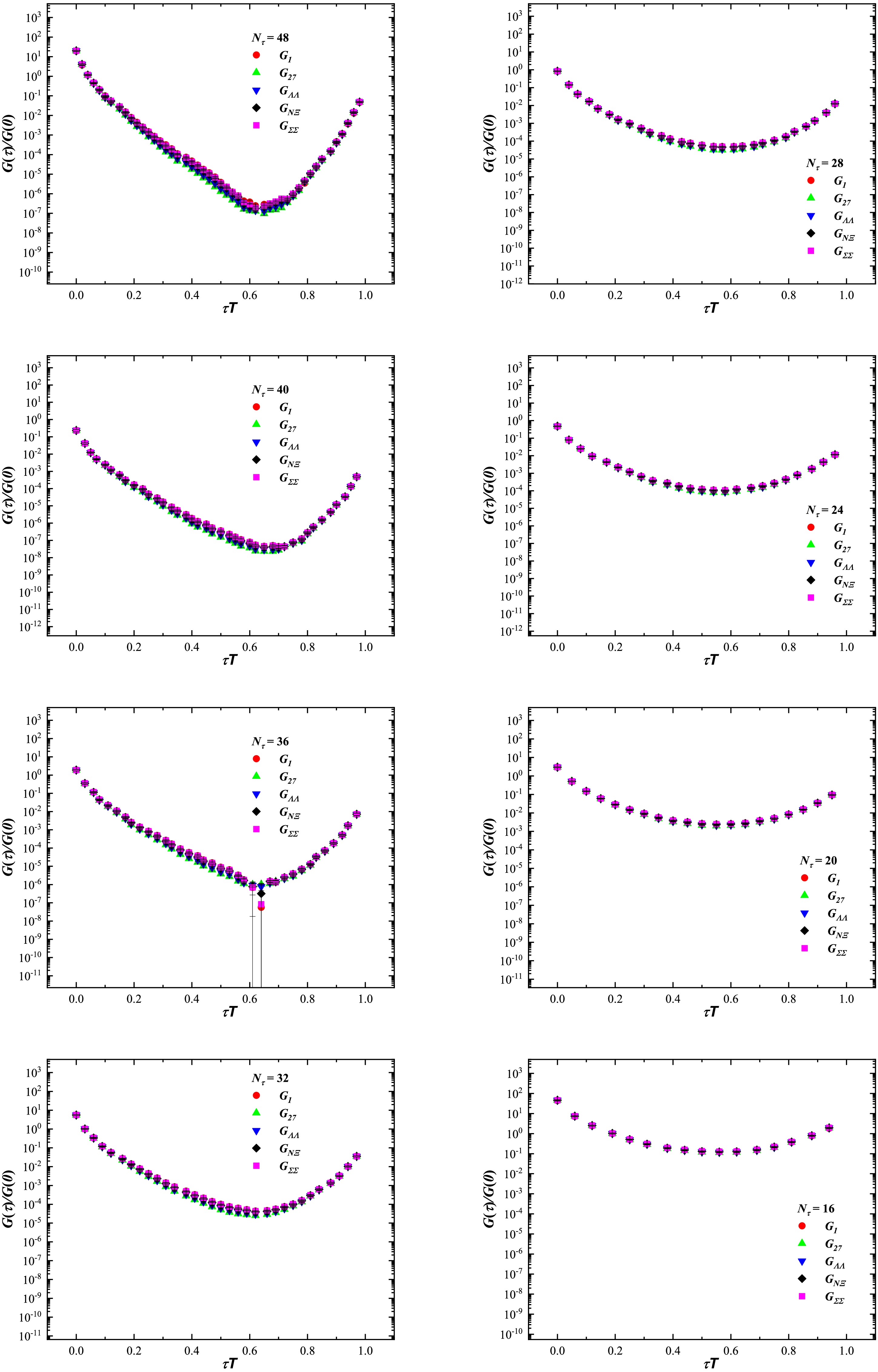
Figure B1. (color online) Euclidean correlators
$ G(\tau)/G(0) $ for$ H_1 $ ,$ H_{27} $ ,$ H_{\Lambda\Lambda} $ ,$ H_{N\Xi} $ , and$ H_{\Sigma\Sigma} $ as functions of$ \tau T $ on the eight lattices. The vertical axis is logarithmic. -
Figure B1. (color online) Euclidean correlators
$ G(\tau)/G(0) $ for$ H_1 $ ,$ H_{27} $ ,$ H_{\Lambda\Lambda} $ ,$ H_{N\Xi} $ , and$ H_{\Sigma\Sigma} $ as functions of$ \tau T $ on the eight lattices. The vertical axis is logarithmic. -
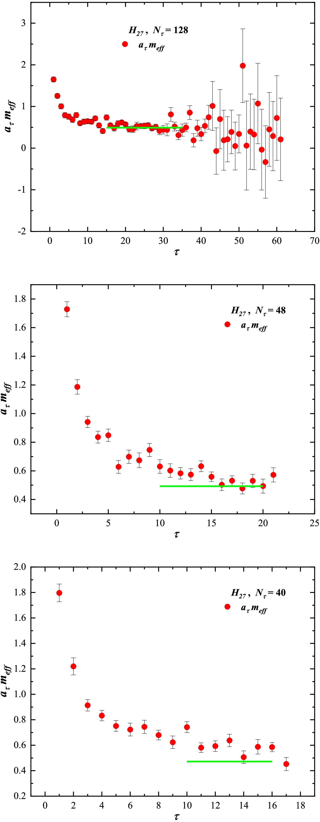
Figure C1. (color online) Effective mass of
$ H_{27} $ on the$ N_\tau = 128, 48, 40 $ lattices. The green line represents the extrapolated mass value from Table 3.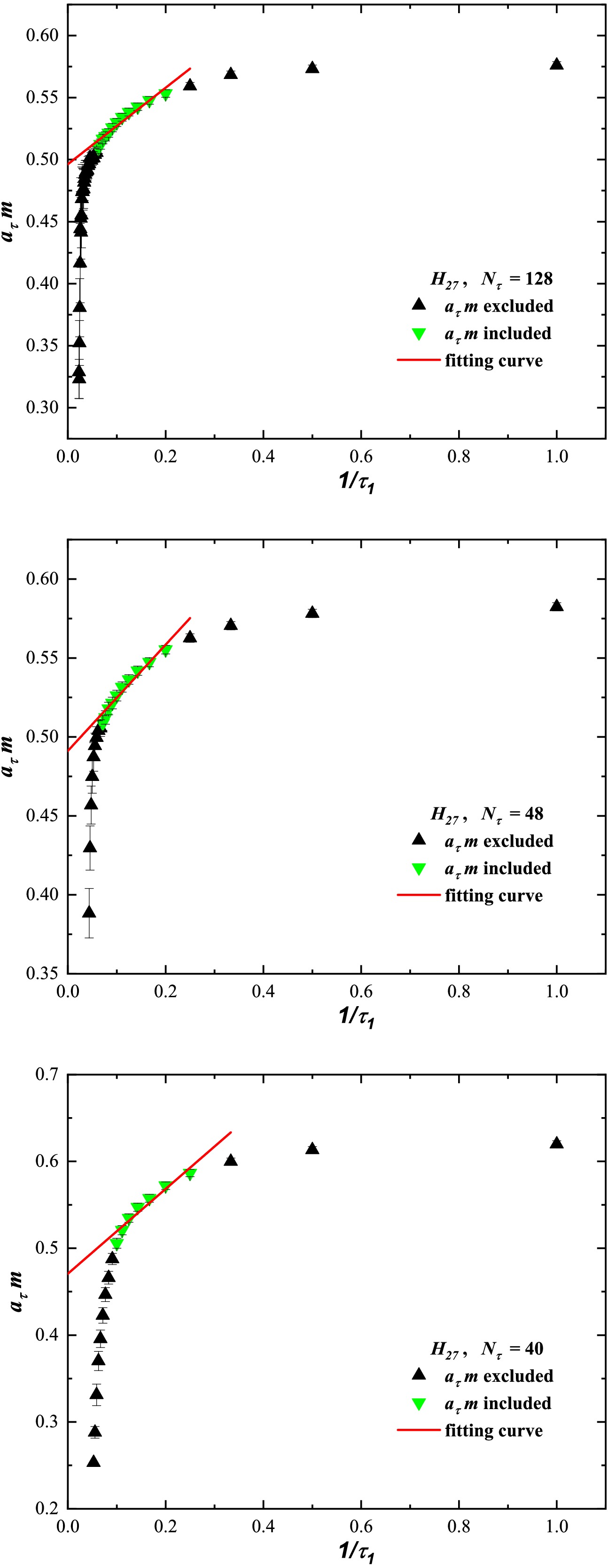
Figure C2. (color online) Linear fit of
$ a_\tau m $ versus$ 1/\tau_1 $ for one bootstrap group of$ H_{27} $ correlators on the$ N_\tau = 128 $ ,$ 48 $ , and$ 40 $ lattices. The$ a_\tau m $ value at$ \tau_1 = 0 $ is not shown.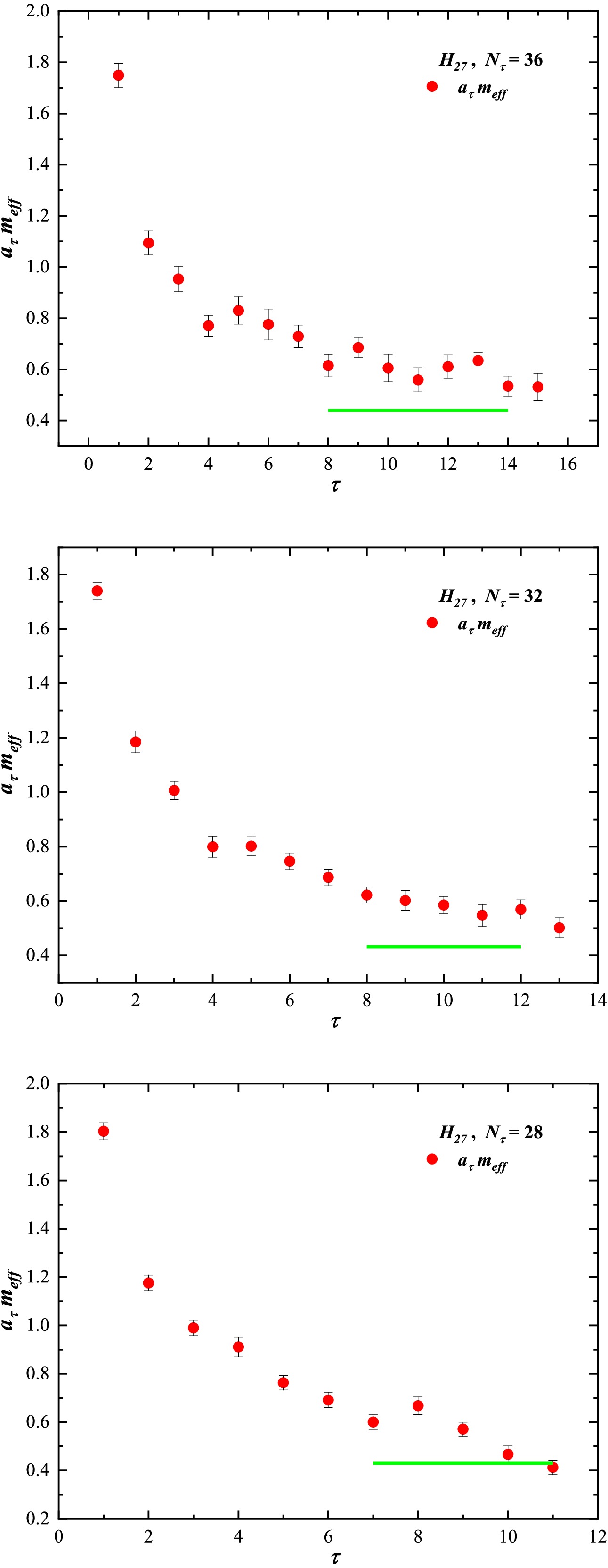
Figure C3. (color online) Effective mass of
$ H_{27} $ on the$ N_\tau = 36, 32, 28 $ lattices. The green line represents the extrapolated mass value from Table 3.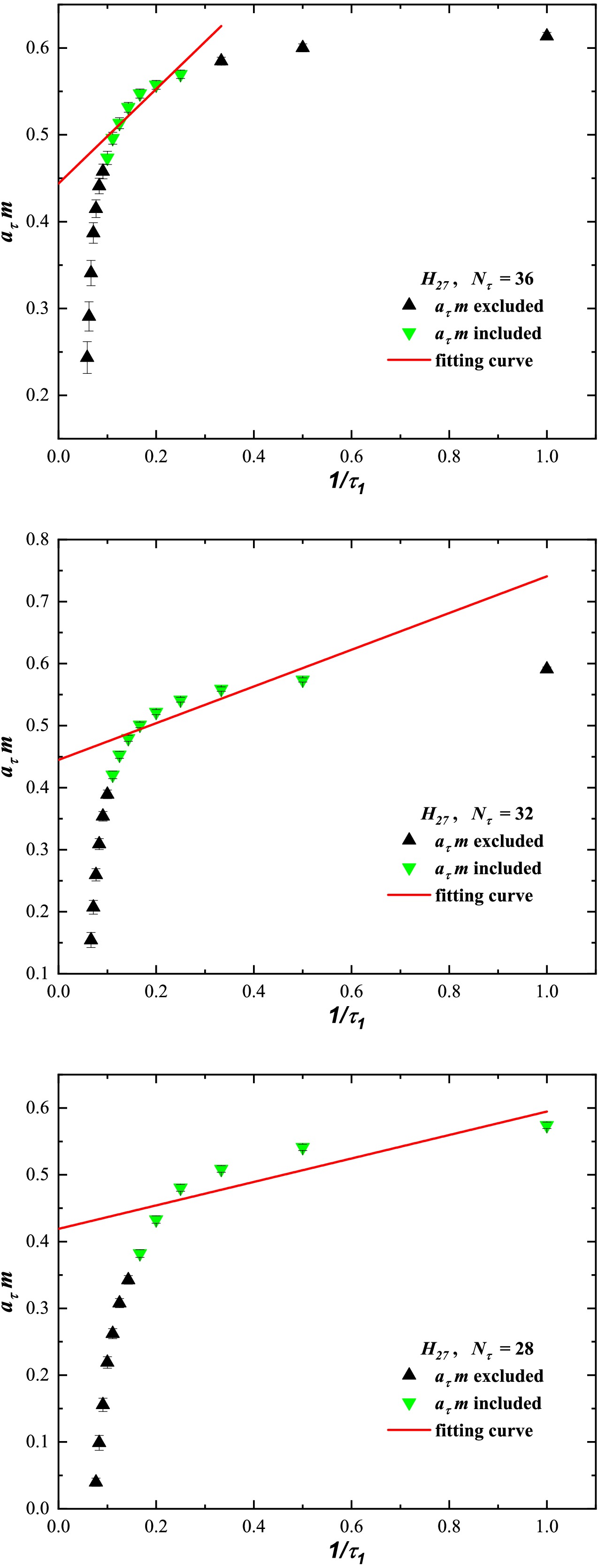
Figure C4. (color online) Linear fit of
$ a_\tau m $ versus$ 1/\tau_1 $ for one bootstrap group of$ H_{27} $ correlators on the$ N_\tau = 36 $ ,$ 32 $ , and$ 28 $ lattices. The$ a_\tau m $ value at$ \tau_1 = 0 $ is not shown.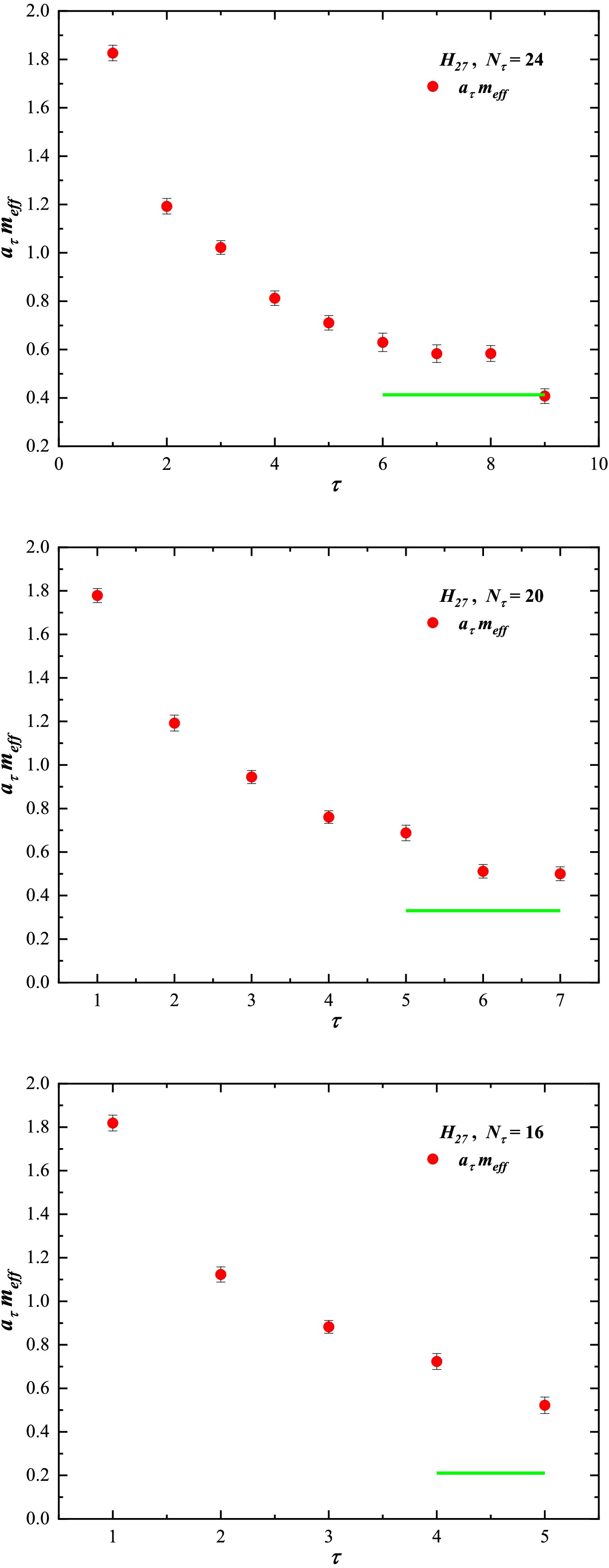
Figure C5. (color online) Effective mass of
$ H_{27} $ on the$ N_\tau = 24, 20, 16 $ lattices. The green line represents the extrapolated mass value from Table 3.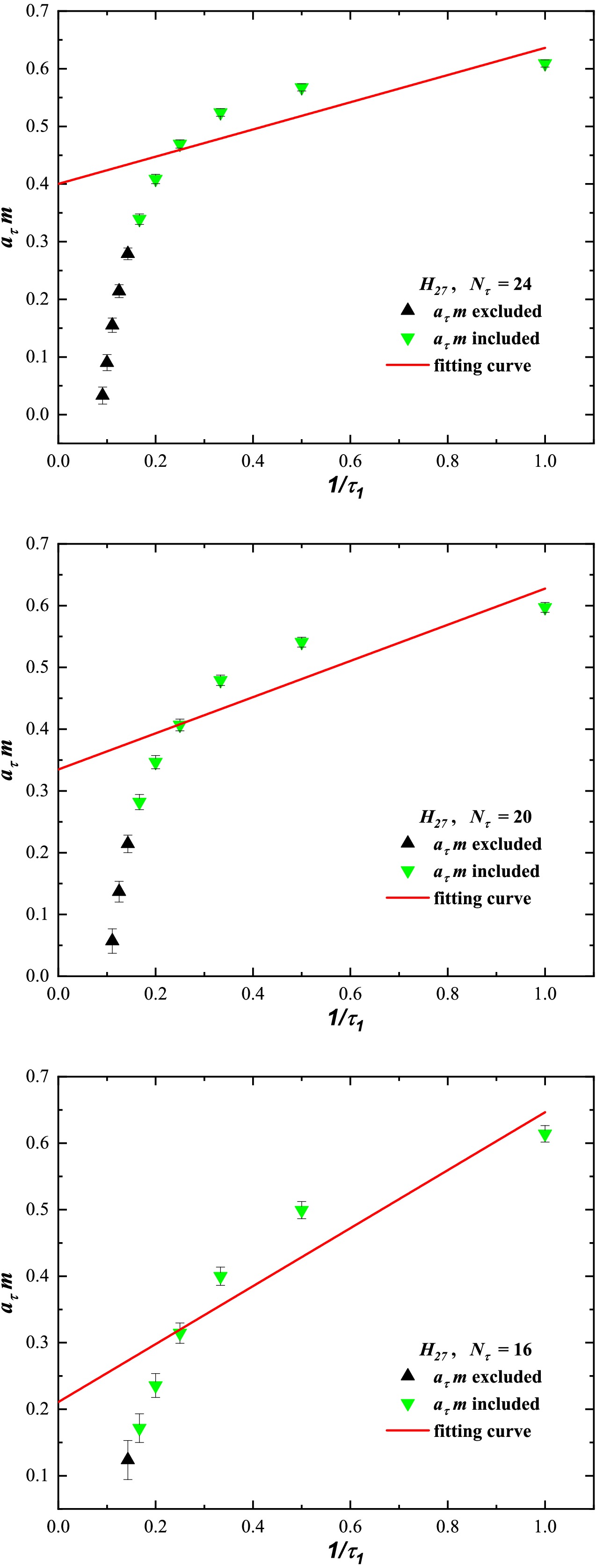
Figure C6. (color online) Linear fit of
$ a_\tau m $ versus$ 1/\tau_1 $ for one bootstrap group of$ H_{27} $ correlators on the$ N_\tau = 24 $ ,$ 20 $ , and$ 16 $ lattices. The$ a_\tau m $ value at$ \tau_1 = 0 $ is not shown.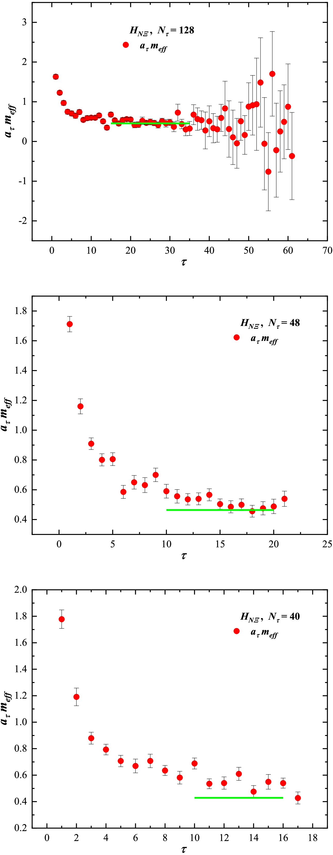
Figure C7. (color online) Effective mass of
$ H_{N\Xi} $ on the$ N_\tau = 128, 48, 40 $ lattices. The green line represents the extrapolated mass value from Table 3.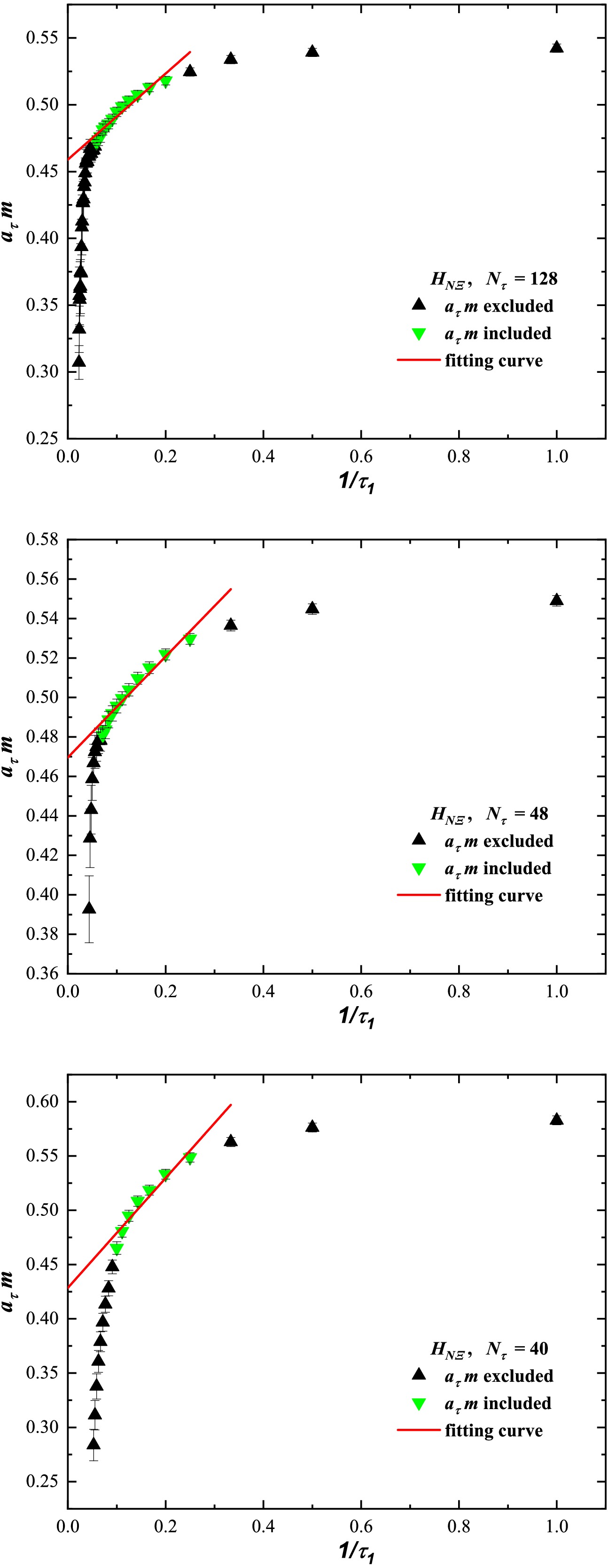
Figure C8. (color online) Linear fit of
$ a_\tau m $ versus$ 1/\tau_1 $ for one bootstrap group of$ H_{N\Xi} $ correlators on the$ N_\tau = 128 $ ,$ 48 $ , and$ 40 $ lattices. The$ a_\tau m $ value at$ \tau_1 = 0 $ is not shown.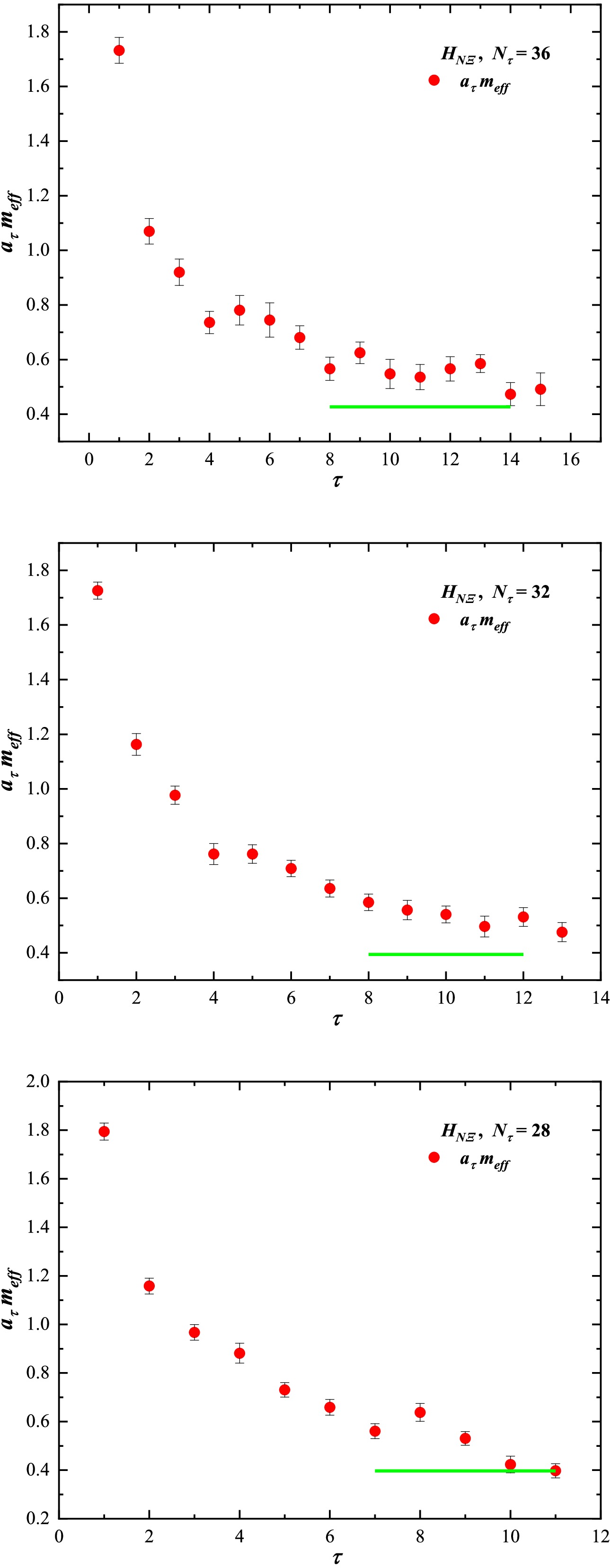
Figure C9. (color online) Effective mass of
$ H_{N\Xi} $ on the$ N_\tau = 36, 32, 28 $ lattices. The green line represents the extrapolated mass value from Table 3.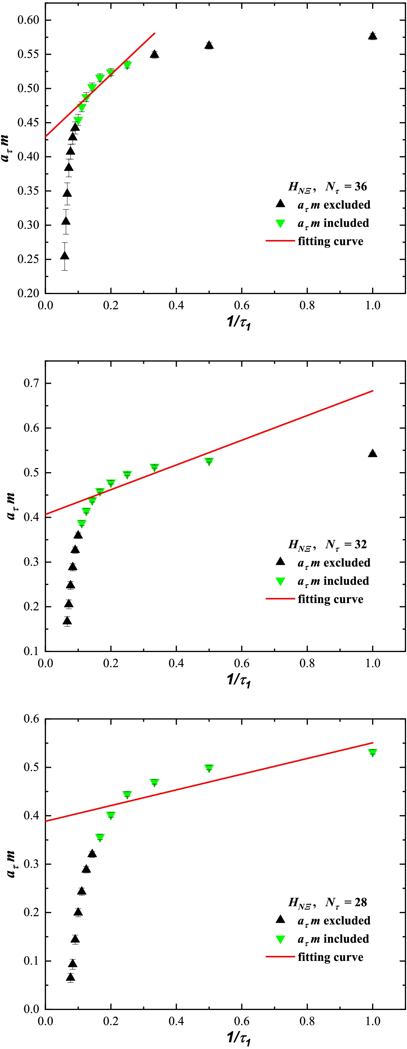
Figure C10. (color online) Linear fit of
$ a_\tau m $ versus$ 1/\tau_1 $ for one bootstrap group of$ H_{N\Xi} $ correlators on the$ N_\tau = 36 $ ,$ 32 $ , and$ 28 $ lattices. The$ a_\tau m $ value at$ \tau_1 = 0 $ is not shown.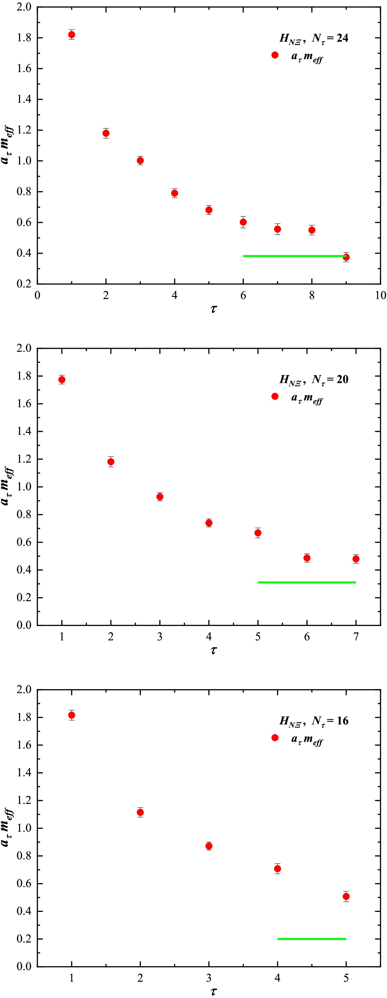
Figure C11. (color online) Effective mass of
$ H_{N\Xi} $ on the$ N_\tau = 24, 20, 16 $ lattices. The green line represents the extrapolated mass value from Table 3.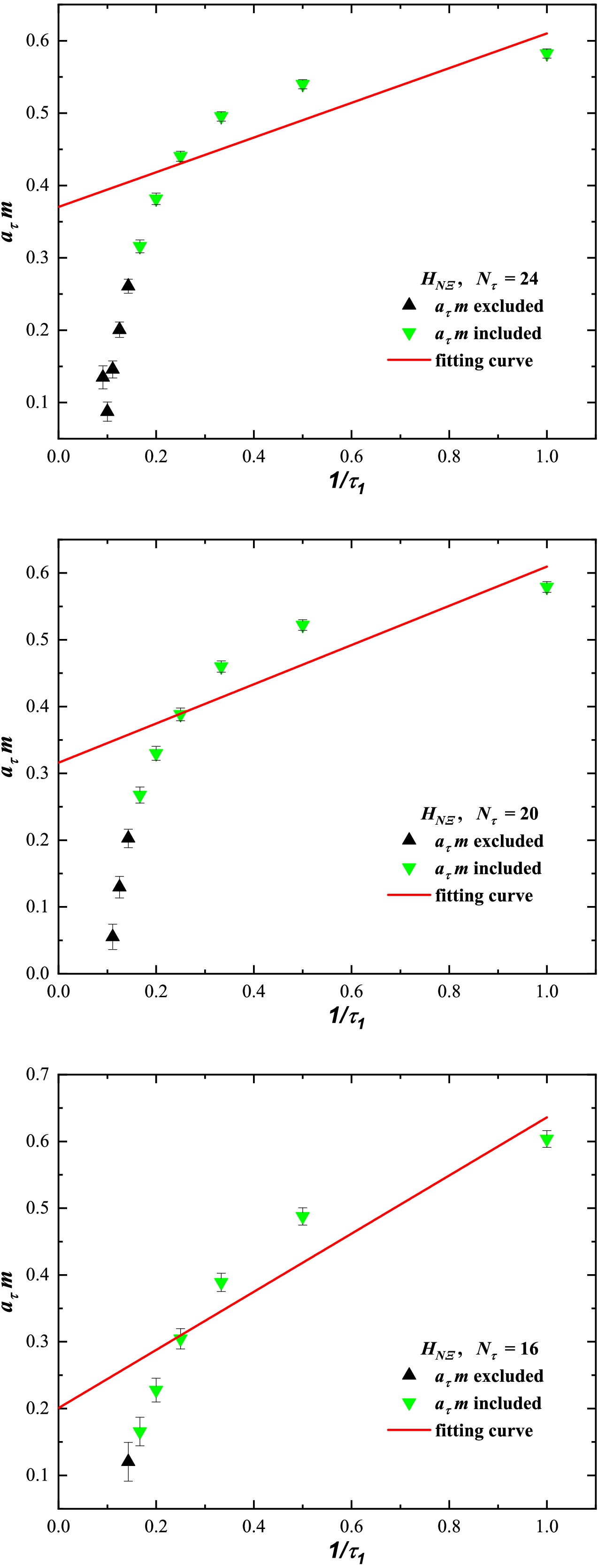
Figure C12. (color online) Linear fit of
$ a_\tau m $ versus$ 1/\tau_1 $ for one bootstrap group of$ H_{N\Xi} $ correlators on the$ N_\tau = 24 $ ,$ 20 $ , and$ 16 $ lattices. The$ a_\tau m $ value at$ \tau_1 = 0 $ is not shown. -
Figure C1. (color online) Effective mass of
$ H_{27} $ on the$ N_\tau = 128, 48, 40 $ lattices. The green line represents the extrapolated mass value from Table 3.
Figure C2. (color online) Linear fit of
$ a_\tau m $ versus$ 1/\tau_1 $ for one bootstrap group of$ H_{27} $ correlators on the$ N_\tau = 128 $ ,$ 48 $ , and$ 40 $ lattices. The$ a_\tau m $ value at$ \tau_1 = 0 $ is not shown.
Figure C3. (color online) Effective mass of
$ H_{27} $ on the$ N_\tau = 36, 32, 28 $ lattices. The green line represents the extrapolated mass value from Table 3.
Figure C4. (color online) Linear fit of
$ a_\tau m $ versus$ 1/\tau_1 $ for one bootstrap group of$ H_{27} $ correlators on the$ N_\tau = 36 $ ,$ 32 $ , and$ 28 $ lattices. The$ a_\tau m $ value at$ \tau_1 = 0 $ is not shown.
Figure C5. (color online) Effective mass of
$ H_{27} $ on the$ N_\tau = 24, 20, 16 $ lattices. The green line represents the extrapolated mass value from Table 3.
Figure C6. (color online) Linear fit of
$ a_\tau m $ versus$ 1/\tau_1 $ for one bootstrap group of$ H_{27} $ correlators on the$ N_\tau = 24 $ ,$ 20 $ , and$ 16 $ lattices. The$ a_\tau m $ value at$ \tau_1 = 0 $ is not shown.
Figure C7. (color online) Effective mass of
$ H_{N\Xi} $ on the$ N_\tau = 128, 48, 40 $ lattices. The green line represents the extrapolated mass value from Table 3.
Figure C8. (color online) Linear fit of
$ a_\tau m $ versus$ 1/\tau_1 $ for one bootstrap group of$ H_{N\Xi} $ correlators on the$ N_\tau = 128 $ ,$ 48 $ , and$ 40 $ lattices. The$ a_\tau m $ value at$ \tau_1 = 0 $ is not shown.
Figure C9. (color online) Effective mass of
$ H_{N\Xi} $ on the$ N_\tau = 36, 32, 28 $ lattices. The green line represents the extrapolated mass value from Table 3.
Figure C10. (color online) Linear fit of
$ a_\tau m $ versus$ 1/\tau_1 $ for one bootstrap group of$ H_{N\Xi} $ correlators on the$ N_\tau = 36 $ ,$ 32 $ , and$ 28 $ lattices. The$ a_\tau m $ value at$ \tau_1 = 0 $ is not shown.
Figure C11. (color online) Effective mass of
$ H_{N\Xi} $ on the$ N_\tau = 24, 20, 16 $ lattices. The green line represents the extrapolated mass value from Table 3.
Figure C12. (color online) Linear fit of
$ a_\tau m $ versus$ 1/\tau_1 $ for one bootstrap group of$ H_{N\Xi} $ correlators on the$ N_\tau = 24 $ ,$ 20 $ , and$ 16 $ lattices. The$ a_\tau m $ value at$ \tau_1 = 0 $ is not shown.
Masses of the conjectured H-dibaryon for different channels at different temperatures
- Received Date: 2026-03-06
- Available Online: 2027-01-15
Abstract: We present a lattice QCD spectroscopy study of the conjectured H-dibaryon in five channels at nine temperatures ranging from $T/T_c =0.24$ to $T/T_c = 1.90$. The five channels are the flavor singlet, flavor 27-plet, $\Lambda \Lambda$, $N \Xi$, and $\Sigma \Sigma$. Five interpolating operators are employed, one for each channel. The simulations are performed on anisotropic lattices with $N_f=2+1$ flavors of clover fermions at a quark mass corresponding to $m_\pi=384(4)\, {\rm MeV} $. The thermal ensembles were provided by the FASTSUM collaboration and the zero-temperature ensembles by the Hadspec collaboration. The simulations show that the H-dibaryon mass in the 27-plet channel is the largest across the nine temperatures, whereas the mass in the $\Sigma \Sigma $ channel is the smallest. We also calculate the spectral density of the H-dibaryon correlation function for the five channels. The spectral density distributions of the five channels exhibit similar behavior. The mass differences $\Delta m = m_H - 2\,m_{\Lambda} $ between the H-dibaryon and a Λ pair at $T/T_c =0.24 $ for the five channels are also estimated. The results show that $\Delta m $ is positive for the 27-plet and $\Lambda \Lambda$ channels, whereas $\Delta m $ is negative for the singlet, $N \Xi$, and $\Sigma \Sigma$ channels. These findings are limited, however, by the use of a single spatial volume and a relatively large quark mass.



 DownLoad: