Interpreting the 95 GeV di-photon and di-tau excesses in the Georgi–Machacek model

The discovery of the 125 GeV Higgs boson by the ATLAS [1] and CMS [2] Collaborations in 2012 confirmed the Standard Model (SM) framework of electroweak symmetry breaking (EWSB). Nevertheless, theoretical motivations and the sizable uncertainties in current Higgs data fits still leave ample room for an extended Higgs sector [3]. Consequently, the search for additional scalar fields remains a crucial objective.

The CMS and ATLAS Collaborations have each reported a di-photon excess around 95.4 GeV [4−6]. A phenomenological combination of these Run-2 di-photon results in [7] finds a local significance of $ 3.1\sigma $ and a combined signal strength $ \mu_{\gamma\gamma}^{\rm{ATLAS+CMS}} = 0.24^{+0.09}_{-0.08} $. CMS has also observed another scalar resonance at 100 GeV with a local significance of $ 3.1\sigma $ [8]. Because the mass resolution in the di-tau channel is poorer than in the di-photon channel, this excess could be compatible with the same scalar as the di-photon excess. At 95 GeV, the local significance in the di-tau channel is 2.6σ, with a signal strength of $ \mu_{\tau\tau}^{\rm{CMS}} = 1.2 \pm 0.5 $. Additionally, data from the Large Electron-Positron Collider (LEP) show an excess at 98 GeV in the $ b\bar{b} $ channel, with a local significance of 2.3σ and a signal strength of $ \mu_{b\bar{b}}^{\rm{LEP}} = 0.117 \pm 0.057 $ [9].

Although each excess is individually modest in significance, their persistence motivates a systematic exploration within well-defined new physics frameworks. Since the three excesses cluster in a similar mass region and exhibit signal strengths comparable to those expected from a SM-like Higgs boson, it is natural to view them as potential hints of an extended Higgs sector in the context of EWSB. It is therefore important to examine whether they can be consistently interpreted as manifestations of a light scalar particle. There is broad theoretical interest in simultaneously explaining the di-photon, di-tau, and $ b\bar{b} $ excesses within a consistent framework. [7, 10, 11] These include scalar extensions [12, 13], dilaton models [14, 15], extra-$ {\rm{U(1)}} $ symmetry [16−20], left-right models [21], triplet Higgs models [22], scotogenic models [23−25], Higgs radion models [26, 27], and other mechanisms [28−30]. Discussions have also been carried out in various versions of the two-Higgs-doublet model (2HDM) [31−44], and in the singlet-extended 2HDM [45−56]. In a supersymmetric framework, the minimal supersymmetric standard model (MSSM) cannot provide a common explanation [57]. By contrast, a well-motivated supersymmetric explanation of the observed excesses is provided by the next-to-minimal supersymmetric standard model (NMSSM), in which a mostly singlet-like Higgs boson can naturally appear around 95 GeV [58−68]. Another concrete example is provided by the $ \mu\nu $SSM, where the $\rm CP$-even right-handed sneutrino may play the role of a light scalar explaining the excesses [69, 70]. Beyond these cases, further supersymmetric scenarios, such as the minimal R-symmetry supersymmetric standard model (MRSSM) [71, 72], have also been explored as possible solutions accommodating a light scalar state. Finally, several works have approached the problem from a collider perspective [73−79].

The Georgi-Machacek (GM) model [80−91] extends the SM by introducing a complex ${{S U(2)}}_L$ triplet scalar χ with hypercharge $ +1 $ and a real ${{S U(2)}}_L$ triplet scalar ξ with hypercharge 0. The field content is arranged such that custodial symmetry is preserved at tree level after EWSB, provided the triplet vacuum expectation values (VEVs) are aligned, $ v_\chi = v_\xi \equiv v_\Delta $. This alignment permits $ v_\Delta $ values up to several tens GeV, significantly larger than in generic triplet extensions, while maintaining $ \rho_{\rm{tree}}=1 $. The model predicts nine additional scalar states, including a characteristic doubly charged Higgs boson, resulting in a rich phenomenology and distinctive collider signatures [92−124]. Notably, the GM model allows the couplings of the SM-like Higgs boson to weak gauge bosons to exceed their SM values [125−127].

The extended scalar sector improves vacuum stability and can induce a strong first-order electroweak phase transition (EWPT), potentially generating gravitational-wave signals accessible to future experiments [128−132]. If lepton number violation is present, triplet-lepton interactions can generate neutrino masses [133−136]. The GM framework has also been employed to address the W-mass anomaly reported by CDF-II [136−139], especially when custodial symmetry-breaking effects are included [140−142]. Furthermore, the light custodial singlet scalar of the GM model constitutes a natural candidate to interpret the excesses observed near 95 GeV [143−147]. An explanation for the excesses observed in the $ \gamma\gamma $, $ \tau\tau $, and $ b\bar{b} $ channels requires a near-degenerate $\rm CP$-even/$\rm CP$-odd ‘twin-peak’ structure [143]; with only a single light $\rm CP$-even state, the $ \tau\tau $ excess is in tension with the $ \gamma\gamma $ and $ b\bar b $ channels [143−145]. Recent analyses, however, strongly disfavor the LEP $ b\bar{b} $ excess as evidence for a new scalar [78], motivating a focus on the LHC-driven $ \gamma\gamma $ and $ \tau\tau $ channels.

The positive-definiteness vacuum stability conditions for the GM model were proposed in [148], which preclude the existence of deeper vacua in large-field regions. Moving beyond the conventional tree-level analysis, the study employs the one-loop renormalization group-improved (RG-improved) effective potential, along with a novel criterion for the positive definiteness of homogeneous polynomials in multiple variables—a refinement necessitated by loop-induced custodial symmetry-breaking effects. Through numerical analysis, it is shown that the quartic coupling ranges permitted by the positive-definiteness requirements significantly deviate from those derived from tree-level bounded-from-below conditions. Notably, certain parameter regions previously excluded by tree-level criteria become viable when the one-loop RG-improved scalar potential is considered. Conversely, some regions of parameter space that satisfy tree-level bounded-from-below constraints at the electroweak scale are ultimately ruled out by the positive-definiteness requirements of the effective potential in large-field regions.

The distinctive aim of this work is to quantify how the one-loop RG-improved positive-definiteness condition affects a single light $\rm CP$-even scalar interpretation of the LHC $ \gamma\gamma $ and $ \tau\tau $ indications. Relative to Ref. [144] (tree-level BFB), the viable di-tau strength is enlarged from $ {\cal{O}}(0.1) $ to $ \sim0.5 $; relative to Ref. [145], the LEP $ b\bar b $ excess is not used as a fitting input; and unlike Ref. [143], we retain one light $\rm CP$-even scalar rather than a twin-peak construction. The CMS di-tau central value remains inaccessible because of tension with the $ 125\; \mathrm{GeV} $ Higgs couplings.

This work is organized as follows. In Sec. II, we provide a brief review of the GM model. A short discussion of the di-photon and di-tau excess signals around 95 GeV is presented in Sec. III. Theoretical and experimental constraints relevant to realistic studies within the GM model are detailed in Sec. IV. Numerical results are displayed in Sec. V. Finally, we present our conclusions in Sec. VI.

The GM model augments the SM scalar sector by introducing additional triplet fields. It contains the familiar ${{S U(2)}}_L$ doublet $ ({\phi}^+,\; {\phi}^0) $ with hypercharge $ 1/2 $, a complex triplet $ ({\chi}^{++},\; {\chi}^{+},\; {\chi}^{0}) $ with hypercharge $ +1 $, and a real triplet $ ({\xi}^{+},\; {\xi}^{0},\; -{\xi}^{+*}) $ with zero hypercharge. This field content allows custodial ${{S U(2)}}_V$ symmetry at tree level and leads to distinctive scalar phenomenology.

To clarify custodial symmetry, the doublet and triplets are arranged into the matrices Φ and ∆, respectively:

The most general scalar potential for the GM scalar sector, constructed to be invariant under a global $ {{S U(2)}}_L \times{{S U(2)}}_R $ symmetry and, consequently, also under its gauged subgroup $ {{S U(2)}}_L \times{{U(1)}}_Y $, reads

Here, $ \sigma^i $ denote the Pauli matrices, and $ T^i $ denote the ${{S U(2)}}$ generators in the triplet representation:

The P matrix rotates the triplet fields ∆ into the Cartesian basis

Note that the last two terms in Eq. (2) vanish under a $ {\mathbb{Z}}_2 $ symmetry. However, we retain them in this work.

Under ${S U(2)}_L \times{S U(2)}_R$, the fields Φ and ∆ transform as

Here, $ U_{L,R} $ denotes $ \exp( \mathrm{i} \theta^a_{L,R} \sigma^a) $ for the doublet and $ \exp( \mathrm{i} \theta^a_{L,R} T^a) $ for the triplet. The SM electroweak gauge group ${S U(2)}_L \times{{U(1)}}_Y$ is embedded in the global ${S U(2)}_L \times{S U(2)}_R$ symmetry, where ${S U(2)}_L$ is identified with the generators $ T_L^i $ and the hypercharge ${{U(1)}}_Y$ is associated with the generator $ T_R^3 $.

After EWSB, the neutral scalar fields can be parameterized as

Here, the parameters $ v_{\xi} $, $ v_{\phi} $, and $ v_{\chi} $ denote the VEVs of the corresponding neutral components of these scalar fields. Then, the tree-level ρ parameter of the GM model can be expressed as

Therefore, when the triplet VEVs are aligned, $ v_\chi = v_\xi \equiv v_\Delta $, the vacuum is invariant only under the diagonal (custodial) subgroup ${S U(2)}_V \subset{S U(2)}_L \times{S U(2)}_R$ (i.e., when $ U_L = U_R $). Consequently, the tree-level ρ parameter automatically satisfies $ \rho_{\rm{tree}} = 1 $. In this alignment limit, the VEVs of the scalar fields take the form

The condition for EWSB is given by

The physical scalars are then decomposed into irreducible representations under the custodial ${S U(2)}_V$ symmetry. The doublet Φ (interpreted as a $ {\bf{2}} \otimes{\bf{2}} $ representation) decomposes into $ {\bf{1}} \oplus{\bf{3}} $, whereas the triplet ∆ (as a $ {\bf{3}} \otimes{\bf{3}} $ representation) decomposes into $ {\bf{1}} \oplus{\bf{3}} \oplus{\bf{5}} $. One triplet, $ G_3 $, provides the Nambu-Goldstone bosons eaten by the W and Z bosons

where the mixing parameter $ \theta_H $ is defined as

The singlet $ H_1^0 $ (originating from the ∆ field), the triplet ($ H_3^{\pm} $ and $ H_3^0 $), and the quintuplet ($ H_5^{\pm\pm} $, $ H_5^{\pm} $, and $ H_5^0 $) are given by

In the basis $ (h_\phi, H_1^0, H_5^0) $, the mass matrix for the $ CP $-even Higgs states is given by

where the elements of the $ 2\times 2 $ block are

The mass eigenstates h and H are defined by

where the mixing angle α is defined by

The masses of all Higgs mass eigenstates can then be expressed as

By applying the tadpole conditions

The mass parameters $ m_{\phi}^2 $ and $ m_{\Delta}^2 $ in Eq. (2) can be eliminated as follows:

In summary, the free parameters of the GM model consist of five dimensionless couplings $ \lambda_{1,2,3,4,5} $, two dimensional parameters $ \mu_{1,2} $, and one mixing parameter $ \theta_H $. In this work, we adopt the following set of free parameters in practice:

where $ \mu_{1,2} $ are replaced by $ m_{h,H}^{\rm{In}} $, and $ \lambda_1 $ is replaced by α. In the following sections, $ m_{h,H} $ without a superscript denotes the physical pole mass as calculated by the spectrum calculator.

In the setup introduced in Sec. II, the GM model contains two light singlet scalar fields. In this work, the heavier state, denoted by h, is identified with the $ 125\; \mathrm{GeV} $ SM-like Higgs boson. The other state, denoted by H, serves as a candidate to explain the observed excesses around $ 95\; \mathrm{GeV} $. The couplings of these Higgs states to SM fermions (f) and weak gauge bosons ($ V = W, Z $) are modified as follows:

with the effective Higgs couplings κ at leading order

Using this framework, the GM predictions for the di-photon signal strength normalized to the SM prediction, $ \mu_{\gamma\gamma} $, are given by

where the Higgs-boson mass is fixed at approximately 95 GeV (denoted by $ H_{95} $ and $ h_{95} $), and the subscript GM (SM) denotes the GM (SM) prediction for the inclusive production rate of $ H_{95} $ ($ h_{95} $). The specific value $ 1.39\times 10^{-3} $ is the SM Higgs branching ratio at 95 GeV, as calculated by the LHC Higgs Cross Section Working Group [149]. The approximation in the second line arises because SM Higgs production is dominated by the gluon-gluon fusion process, which accounts for approximately 89% of the total Higgs production at a mass of 95 GeV [149]. The third line follows because the gluon-gluon fusion process ($ gg \to h $) is mediated by a colored-fermion loop. As a result, the effective coupling $ \kappa^{H}_{gg} $ equals $ \kappa^{H}_{F} $, since the fermionic couplings of H scale universally as $ \kappa_{F}^{H} $ at leading order, as shown in Eq. (22). Similarly, the GM predictions for the signal strengths in the $ \tau\tau $ and $ bb $ channels are given by

From the above definitions, all signal strengths are expressed in terms of the ratio $ \sigma_{\rm{GM}}/\sigma_{\rm{SM}} $, so QCD corrections to the numerator and denominator largely cancel. This reduces the theoretical uncertainty in the predicted signal strengths. The LEP $ b\bar b $ relation is exact at leading order (Higgsstrahlung $ \propto|\kappa_V^H|^2 $). The inclusive LHC $ \tau\tau $ relation is approximate: it assumes gluon-fusion dominance and neglects smaller $ \kappa_V^H $-dependent production modes.

We now examine the branching ratios. The partial decay width of the lighter scalar H into SM final states can be expressed as

where $ \Gamma_{\rm{SM}} (h\to XX)\big|_{m_h = m_H} $ is the SM Higgs partial decay width evaluated at the mass $ m_H $. Therefore, the total decay width of the custodial-singlet state H can be written as

where the SM Higgs total decay width $ \Gamma^{\rm{SM}}_{h} $ and branching ratios $ {\cal{B}}_{\rm{SM}} \left( h \to XX \right) $ are evaluated at $ m_{H} $. The couplings of the neutral scalars H and h to photons are induced by charged-particle loops. In the SM, Higgs-boson decay into two photons is mediated by W-boson and heavy charged-fermion loops, dominated by the top quark. In the GM model, loops of heavy charged Higgs states $ S_i $ (including $ H_{5}^{\pm\pm} $, $ H_{5}^{\pm} $, and $ H_{3}^{\pm} $) can significantly enhance the partial decay width $ \Gamma(H\to \gamma\gamma) $. The corresponding effective coupling $ \kappa^{H}_{\gamma\gamma} $ can be expressed as

where $ g_{HS_iS_i} $ are the scalar trilinear couplings of H to the charged states $ S_i $, and the loop functions $ A_{0, 1/2, 1} $ can be found in the literature [84, 150, 151]. For an H boson with mass $ 95\; {{\rm{GeV}}} $, $ A_1 \simeq -7.6 $ and $ A_{1/2} \approx 4/3 $. The factor $ A_0 $ reaches its maximum value of $ 1.5 + \mathrm{i} $ at $ m_H = 2 m_{S_i} $, while in the limit of very heavy loop charged scalars, $ A_0(0) \simeq 1/3 $.

Then, the signal strength in Eq. (23) and Eq. (24) can be rewritten as:

It is clear that all three signal strengths share a common factor, $ \left| \kappa^{H}_{F} \right|^2 \cdot \dfrac{\Gamma_{h}^{\rm{SM}}}{\Gamma^{\rm{tot}}_{H}} $. This creates tension in attributing all observed excesses to a single source. Charged scalar states in the GM model can provide positive contributions to the $ \gamma\gamma $ excess, especially the doubly charged $ H_5^{\pm\pm} $ with $ Q_S^2 = 4 $. Ref. [144] investigates various possibilities for H to explain the $ \gamma\gamma $, $ \gamma\gamma + bb $, and $ \gamma\gamma + bb + \tau\tau $ excesses. However, recent dedicated reanalyses argue that this feature is unlikely to arise from a genuine new scalar resonance [78]. Given the limited di-jet mass resolution at LEP and these updated conclusions, we do not attempt to accommodate the $ b\bar b $ hint in this work. Instead, we focus on the two LHC-driven channels ($ \gamma\gamma $ and $ \tau\tau $), where the experimental systematics and resolutions are better controlled in the relevant mass window. Finally, we note that all loop-induced rates, branching ratios, and total widths in our scan are evaluated with the spectrum tools described in Sec. IV.

To realize a light custodial-singlet scalar H near $ 95.4\; {{\rm{GeV}}} $ that can accommodate the LHC hints in the $ \gamma\gamma $ and $ \tau\tau $ channels, we perform a comprehensive parameter scan. This section describes the scan methodology together with the various constraints imposed. The detailed numerical results corresponding to these constraints will be presented in Sec. V.

In practice, we use the package $ \mathrm{GMCALC}$ [152], a dedicated calculator for the GM model. Alternatively, we use the $ \mathrm{SPheno}$ package [153, 154] in combination with $ \mathrm{SARAH}$ [155−159] to compute the GM model spectrum.

We carry out a comprehensive parameter scan using the JARVIS-HEP framework [160]. The input parameters in Eq. (20) are scanned over the following ranges:

To assess the overall viability of the GM model in explaining the observed excesses, we construct a likelihood-based framework. The total likelihood $ {\cal{L}}_{\rm{tot}} $ is defined as

The total $ \chi^2_{\rm{tot}} $ includes only genuine likelihood contributions from the experimental observables, whereas the factors $ \Theta_{\rm{PD}} $, $ \Theta_{\rm{unit}} $, $ \Theta_{\tt{HB}} $, and $ \Theta_{\tt HS} $ serve as acceptance criteria that restrict the likelihood support to theoretically and phenomenologically viable regions of parameter space.

The individual $ \chi^2 $ and Θ terms entering Eq. (30) are defined below.

● $\chi^2_{\rm{mass}} = \left( \dfrac{m_h - 125.18\; {\rm{GeV}}}{1\; {\rm{GeV}}} \right)^2 + \left( \dfrac{m_H - 95.4\; {\rm{GeV}}}{1\; {\rm{GeV}}} \right)^2$.

Here, $ m_h $ and $ m_H $ denote the theoretically predicted masses of the two $\rm CP$-even Higgs states, and the total uncertainties, including both theoretical and experimental contributions, are each set to $ 1\; {{\rm{GeV}}} $.

● $ \Theta_{\tt{HB}} $ implements the direct-search constraints from $ \mathrm{HiggsBounds-5.10.0}$ [161−165]. We define $ \Theta_{\tt{HB}}=1 $ for parameter points that pass the HiggsBounds exclusion test and $ \Theta_{\tt{HB}}=0 $ otherwise. In this way, the direct-search constraints act as a veto on the parameter space rather than as a compensating contribution to the global $ \chi^2 $.

● $ \Theta_{\tt HS} $ encodes the consistency requirement from $ \mathrm{HiggsSignals-2.6.2}$ [161, 166−168]. To avoid double counting Higgs signal-strength information with the explicit $ \chi^2_{\kappa} $ term defined below, we do not include the $ \mathrm{HiggsSignals}$ output as an additive likelihood contribution to $ \chi^2_{\rm{tot}} $. Instead, we require the sample to satisfy $ \chi^2({\rm{GM}}) \lt \chi^2({\rm{SM}}) $, where $ \chi^2({\rm{SM}})\approx 152.5 $ denotes the SM reference value returned by $ \mathrm{HiggsSignals}$ for the 125 GeV Higgs rate measurements in our setup. Accordingly, we set $ \Theta_{\tt HS}=1 $ when this condition is satisfied and $ \Theta_{\tt HS}=0 $ otherwise.

● $ \chi^2_{95} = \left( \dfrac{\mu_{\gamma\gamma} - 0.24}{0.09} \right)^2 + \left( \dfrac{\mu_{\tau\tau} - 1.2}{0.5} \right)^2 $ denotes the two excesses at $ 95\; {{\rm{GeV}}} $, where $ \mu_{\gamma\gamma} $ and $ \mu_{\tau\tau} $ are the theoretical predictions including loop corrections.

● The contribution $ \chi^2_{\rm{EW}} $ encodes constraints from electroweak precision measurements in terms of the oblique parameters S, T, and U, which capture the one-loop contributions of the additional scalar states to gauge-boson self-energies and neutral-current processes [169, 170]. In this work, $ \chi^2_{\rm{EW}} $ is implemented using a multivariate Gaussian form

where

and $ \rho_{\rm{EW}} $ denotes the correlation matrix, defined as

In addition, the ρ parameter, which characterizes possible new sources of $ {{S U(2)}} $ breaking beyond the SM Higgs doublet, is constrained to be

In the custodial-symmetric GM setup, $ \rho_{\rm{tree}}=1 $ holds by construction, and any residual deviation arises only at the loop level.

● The contribution $ \chi^2_{\kappa} $ encodes the constraints on the Higgs coupling modifiers through a two-dimensional Gaussian likelihood in the $ (\kappa_V,\kappa_F) $ plane and is defined as

where

and V denotes the corresponding covariance matrix

In our analysis, we use the ATLAS combined fit results shown in Fig. 4 of Ref. [171], namely, $ \hat\kappa_V = 1.035 \pm 0.031 $ and $ \hat\kappa_F = 0.95 \pm 0.05 $, with a correlation coefficient of $ 0.39 $.

● $ \chi_B^2 = \left( \dfrac{{\cal{B}}(B_s\to \mu^+ \mu^-) - 3.1\times{10^{-9}}}{1.3\times{10^{-9}}} \right)^2 + $$ \left( \dfrac{{\cal{B}}(B\to X_s \gamma) - 3.43\times{10^{-4}}}{0.44\times{10^{-4}}} \right)^2 $ accounts for constraints from rare B-meson decays, which are highly suppressed in the SM and therefore provide sensitive probes of physics beyond the SM, particularly extended Higgs sectors [172].

In addition to the experimental limits discussed above, theoretical considerations further constrain the parameter space through the Heaviside step functions $ \Theta_{\rm{unit}} $ and $ \Theta_{\rm{PD}} $ in Eq. (30). These functions act as strict vetoes, restricting the likelihood support to theoretically consistent regions of parameter space, where $ \Theta(x) $ equals one for $ x \ge 0 $ and zero otherwise.

$ \Theta_{\rm{unit}} $ enforces perturbative unitarity in scalar $ 2\to2 $ scattering by requiring the zeroth partial-wave amplitudes to satisfy $ |{\rm{Re}}\,a_0|<\dfrac{1}{2} $ (equivalently $ |a_0|<1 $). In the GM model, this requirement translates into bounds on linear combinations of quartic couplings [173−175], leading to the conditions

Therefore, $ \Theta_{\rm{unit}} = 1 $ if all conditions in Eq. (38) are satisfied simultaneously.

The positive-definiteness requirement is imposed to ensure the stability of the electroweak vacuum, so that the scalar potential remains bounded from below for large field values. Quantum corrections can significantly modify the shape of the scalar potential, potentially leading to violations of the tree-level bounded-from-below (BFB) conditions [173]. Such effects may induce deeper vacua at large field values or render the potential unbounded, implying that the electroweak vacuum preserving custodial symmetry is not the true ground state. This situation is reminiscent of the metastability of the SM electroweak vacuum for a $ 125\; {{\rm{GeV}}} $ Higgs boson.

To address this issue, we impose the positive-definiteness constraints [148] to guarantee the stability of the custodial vacuum by requiring the positivity of certain subdeterminants of the quartic-coupling matrices in the one-loop RG-improved potential. For simplicity, the one-loop RG-improved scalar potential is parameterized by the dimensionless couplings λ, $ \rho_{1,2,\cdots ,5} $, and $ \sigma_{1,2,3,4} $ of the most general ${S U(3)}_C \times{S U(2)}_L \times{{U(1)}}_Y$-invariant GM model. ¹ In the custodial-symmetric limit, these couplings map onto the standard GM quartics $ \lambda_{1,2,\cdots,5} $ as

With these definitions, and when $ \rho_5 $ and $ \sigma_4 $ are small, the positive-definiteness constraints reduce to requiring that all leading principal minors of $ {\cal{V}} $ be strictly positive,

where $ {\cal{V}} $ is defined as

and $ {\cal{V}}_n $ denotes the $ n \times n $ upper-left submatrix of $ {\cal{V}} $. Therefore, $ \Theta_{\rm{PD}} $ in Eq. (30) is defined as

In practice, the full matrix is used in numerical calculations, whereas the analytic form shown here corresponds to the simplified limit.

It should be noted that the coupling parameters (such as λ, $ \rho_{1,2,\cdots ,5} $, and $ \sigma_{1,2,3,4} $) must be replaced by their renormalization-group-evolved values in regions of large field values. These evolved parameters can then be used to determine the vacuum structure of the GM model. We utilize the iterative method described in [148] to assess whether the parameter space that adequately explains the observed excess signals satisfies the positive-definiteness constraints. The gauge coupling values at the EW scale used in this study are taken from [176]. To ensure that the vacuum preserves custodial symmetry, the boundary conditions for the scalar quartic couplings at the EW scale, which are crucial for the RGEs, are chosen in accordance with Eq. (39). To determine the scale dependence of the quartic couplings within the one-loop RG-improved tree-level scalar potential, it is essential to evolve the input parameters to an arbitrary scale, especially in regions of large field values, using the appropriate beta functions. In our detailed numerical analysis, to establish the positive-definiteness constraints, we evolve the relevant quartic couplings and dimensionful mass parameters from the EW scale ($ M_Z=91.2\; {{\rm{GeV}}} $) up to the Planck scale ($ M_{\rm{Planck}}\approx 1.12\times{10}^{19}\; {{\rm{GeV}}} $) or to the lowest Landau pole scale, at which any of the quartic couplings diverge.

The tree-level BFB and RG-improved positive-definiteness conditions are not pointwise nested: the former tests the custodial-symmetric quartic potential at the electroweak scale, whereas the latter tracks the general gauge-invariant potential under one-loop evolution to the Planck scale or the first Landau pole. As shown in Refs. [145, 148], the positive-definiteness condition both excludes some regions allowed by BFB and admits some previously excluded regions, yielding a net expansion of the viable parameter space for the $ 95\; \mathrm{GeV} $ excesses.

To ensure a numerically reliable assessment of the GM model's ability to simultaneously explain the two observed excesses, we conducted an extensive exploration of the parameter space using a combination of random scans, Markov Chain Monte Carlo (MCMC) techniques, and MultiNest sampling. These complementary methods provide both broad global coverage and efficient identification of phenomenologically relevant regions with higher likelihood. The final profile-likelihood sample contains $ {\cal{O}}(10^{8}) $ retained points after all selections. Convergence was confirmed by verifying the stability of the profile likelihood (PL) under additional sampling.

In this section, we present detailed results from our sampling. For clarity, we exclude all samples that fail the $ \mathrm{HiggsBounds}$ or $ \mathrm{HiggsSignals}$ consistency requirements, the positive-definiteness requirement, or the perturbative unitarity constraints. Thus, all samples shown in the figures satisfy $ \Theta_{\tt{HB}}=1 $, $ \Theta_{\tt HS}=1 $, $ \Theta_{\rm{PD}}=1 $, and $ \Theta_{\rm{unit}}=1 $.

Figure 1 shows the profile likelihood in the $ (\mu_{\gamma\gamma},\,\mu_{\tau\tau}) $ plane for the $ 95\; \mathrm{GeV} $ scalar after applying the constraints of Sec. IV. The preferred region lies near $ \mu_{\gamma\gamma}\sim0.25 $ and $ \mu_{\tau\tau}\sim0.47 $: the diphoton excess is accommodated near its central value, whereas the ditau excess is only partially reproduced and remains within the experimental $ 2\sigma $ contour.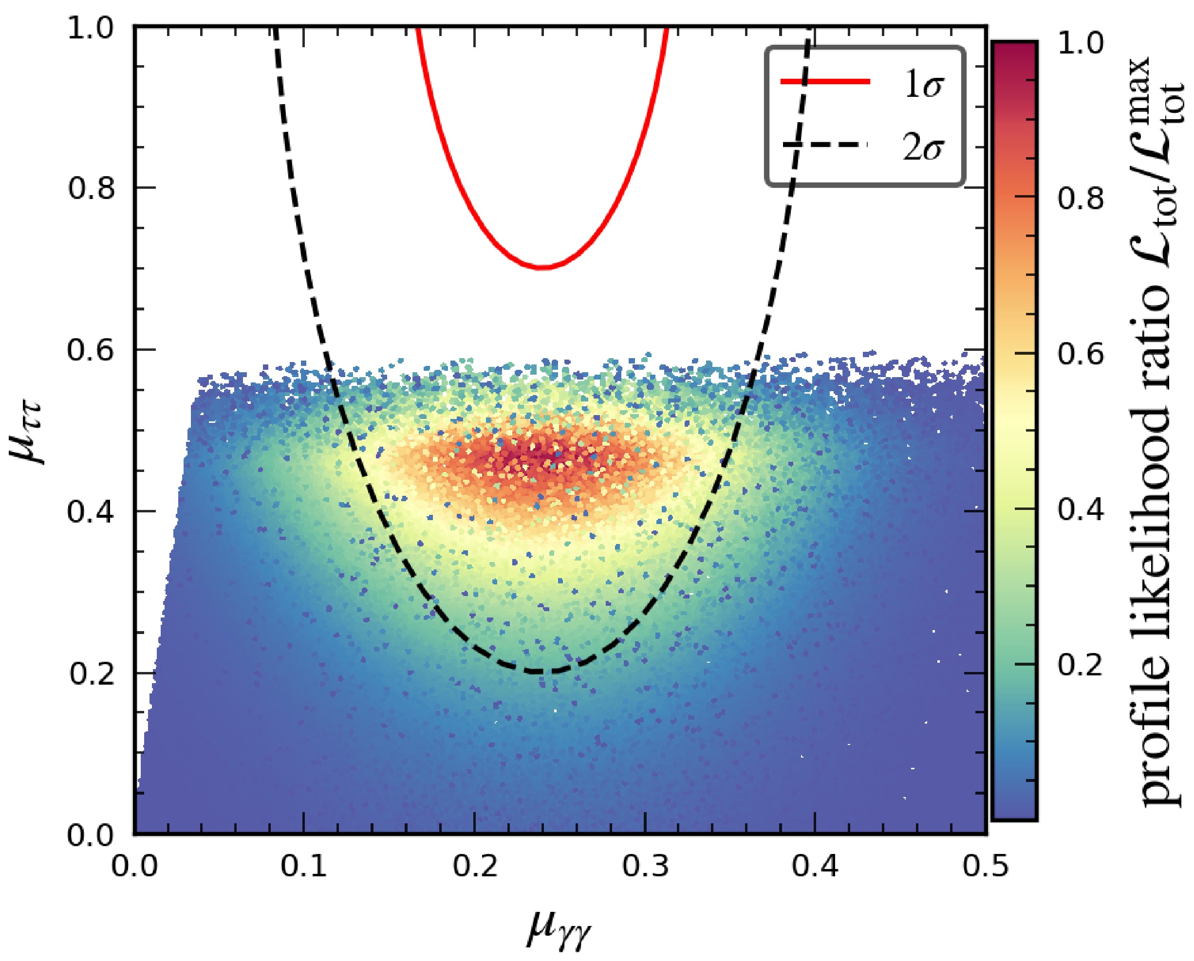

Figure 1.  (color online) Profile likelihood map in the $ (\mu_{\gamma\gamma}, \mu_{\tau\tau}) $ plane. The solid and dashed curves show the experimental $ 1\sigma $ and $ 2\sigma $ contours derived from $ \chi^2_{95} $.

Compared with Ref. [144], where the tree-level BFB analysis mainly populates the region $ \mu_{\tau\tau}\lesssim0.1 $, the RG-improved treatment yields a characteristic ditau signal strength larger by a factor of approximately four to five. Because the scans and likelihoods differ, this should be regarded as a phenomenological cross-check rather than an isolated measure of the vacuum-stability effect.

The inability to fully accommodate the di-tau excess follows from the $ 125\; \mathrm{GeV} $ Higgs-coupling constraints: $ \mu_{\tau\tau} $ cannot be increased independently of $ (\kappa_F,\kappa_V) $, which depend on the common mixing angles α and $ \theta_H $, as shown in Eqs. (24) and (22). Figure 2 (left) shows the resulting narrow $ (\kappa_F,\kappa_V) $ band; $ {\cal{L}}_\kappa $ alone favors $ \mu_{\tau\tau}\sim0.4 $ (middle), whereas the remaining likelihoods prefer larger values (right). Increasing $ |\kappa_F^H| $ also enhances gluon-fusion production and direct-search sensitivity. These competing effects place the combined optimum near the preferred region in Fig. 1 and prevent the fit from approaching the CMS central value.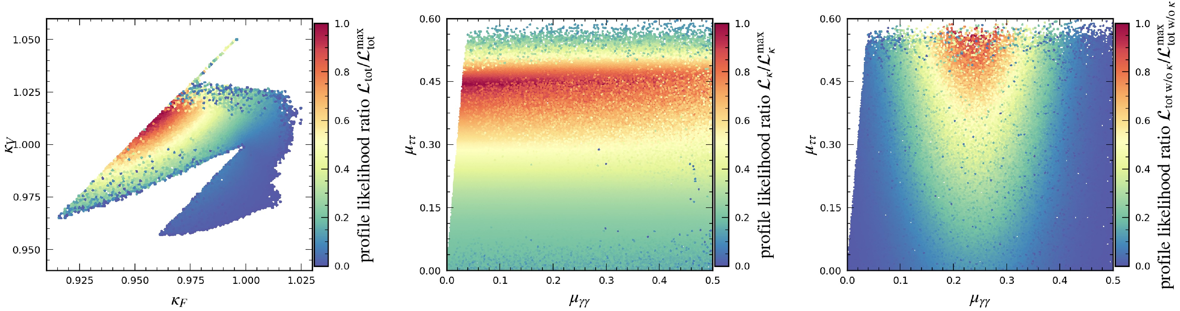

Figure 2.  (color online) Left: The PL map in the $ (\kappa_F, \kappa_V) $ plane. Middle: The PL $ {\cal{L}}_\kappa $ in the $ (\mu_{\gamma\gamma}, \mu_{\tau\tau}) $ plane. Right: The PL $ {\cal{L}}_{\rm{tot}} $, excluding the contribution from $ {\cal{L}}_\kappa $, in the $ (\mu_{\gamma\gamma}, \mu_{\tau\tau}) $ plane.

To highlight the characteristic features of this surviving region, we present three benchmark points in Table 1. $ \mathrm{BP1}$ features a relatively large triplet admixture, with $ \sin\theta_H = 0.131 $ and $ \alpha = -0.808 $. This leads to a significant suppression of the SM-like Higgs coupling $ \kappa_F $. Consequently, the 95 GeV scalar attains a sizable $ \mu_{\tau\tau} = 0.742 $ and the highest diphoton rate among the three points, $ \mu_{\gamma\gamma} = 0.290 $, resulting in the smallest $ \chi^2_{ 95} $. However, it does not satisfy the $ \mathrm{HiggsSignals}$ constraints. $ \mathrm{BP2}$ represents the opposite limit, with a very small triplet VEV, $ \sin\theta_H = 0.029 $. The 125 GeV Higgs is therefore more SM-like. The reduced mixing suppresses the $ \tau\tau $ signal strength to $ \mu_{\tau\tau}=0.525 $, while the diphoton rate, $ \mu_{\gamma\gamma}=0.237 $, is maintained mainly by charged-scalar loop effects. This benchmark satisfies both $ \mathrm{HiggsSignals}$ and $ \mathrm{HiggsBounds}$. Compared with $ \mathrm{BP1}$, $ \mathrm{BP3}$ provides a better solution, with $ \sin\theta_H = 0.125 $ and $ \alpha=-1.040 $, for which $ \kappa_V^h = 0.984 $ is remarkably close to the experimental value. This point achieves a balanced configuration, $ \mu_{\tau\tau}=0.545 $ and $ \mu_{\gamma\gamma}=0.245 $, while remaining consistent with all theoretical and experimental constraints. It exemplifies the thin, correlated region identified in Fig. 2, where the 95 GeV excesses can be accommodated without significantly perturbing the 125 GeV Higgs couplings.

Figure 3 displays the PL projected onto the eight GM model parameter planes. A clear pattern emerges: whereas the quartic couplings $ \lambda_2 $, $ \lambda_3 $, $ \lambda_4 $, and $ \lambda_5 $ span relatively broad ranges, the physically relevant mixing parameters are tightly constrained. In the two $ \lambda_i $ panels, no pronounced minima appear, indicating that the quartic interactions are not strongly constrained individually. Instead, these couplings primarily support the scalar mass spectrum and permit viable loop contributions, without requiring finely tuned correlations among themselves. In contrast, the $ (M_H^{\rm{in}},\alpha) $ projection reveals a highly concentrated high-likelihood region centered at $(95\; {{\rm{GeV}}}, -\dfrac{\pi}{3})$ , corresponding directly to the mass of the observed excess. The narrow range of the mixing angle α is consistent with the data, and large portions of the α parameter space are excluded, indicating that doublet–triplet mixing is tightly constrained.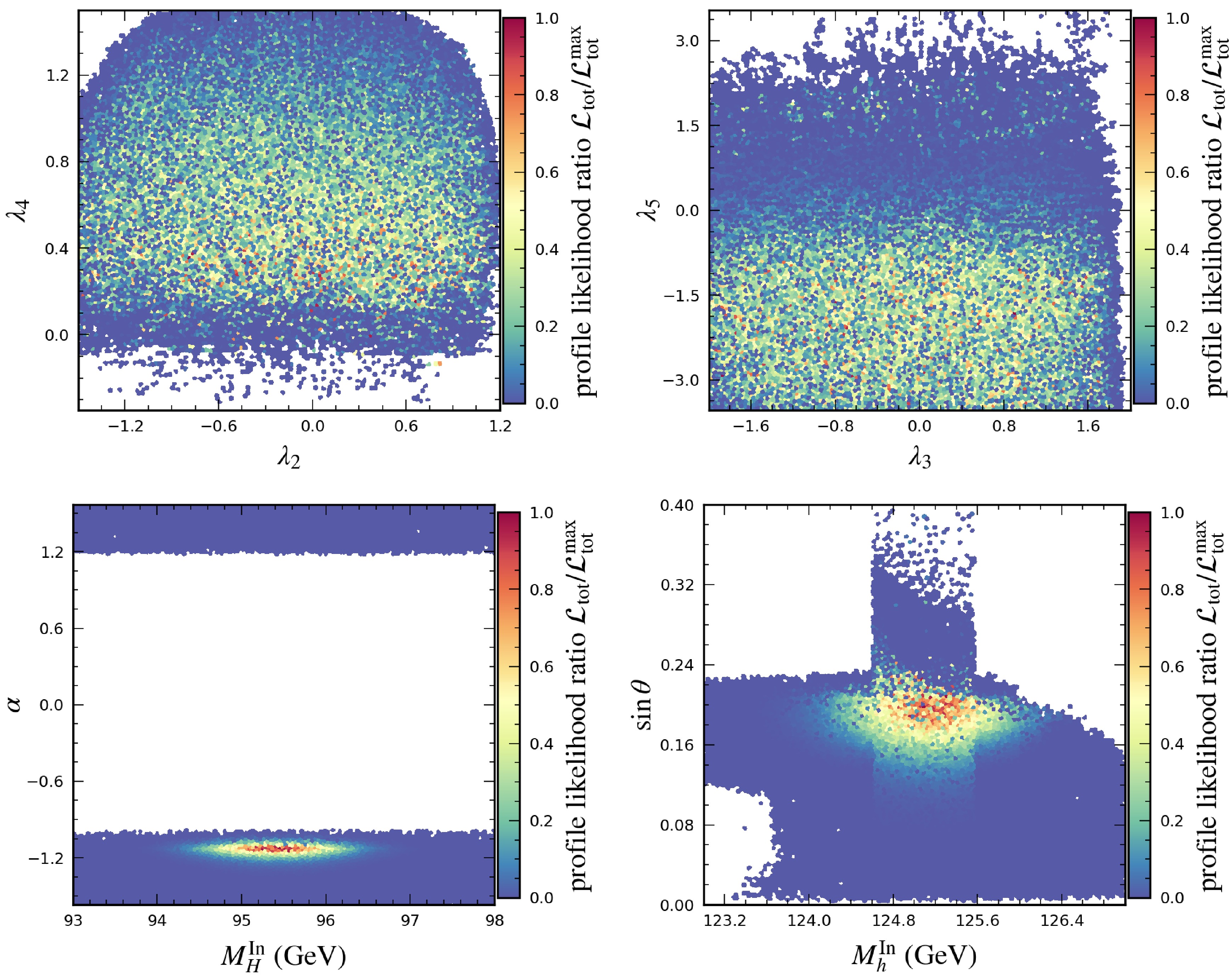

Figure 3.  (color online) Similar to Fig. 1, but shown in the GM model parameter planes.

For values of α with identical magnitude, as shown in the benchmark points $ \mathrm{BP2}$ and $ \mathrm{BP3}$, $ \kappa_F $ remains unchanged, as expected. However, the coupling $ \kappa_V $ associated with positive α is significantly smaller than that for negative α, resulting in a pronounced deviation from the experimental constraints. Moreover, $ \kappa_V^H $ corresponding to positive α is substantially larger than its counterpart for negative α, rendering this scenario incompatible with the additional Higgs-search constraints implemented in the $ \mathrm{HiggsBounds}$ package.

This feature underlies the κ tension observed in Fig. 2: while $\alpha = -\dfrac{\pi}{4}$ would better explain the excess, the overall fit allows only α near $-\dfrac{\pi}{3}$. A similar pattern appears in the $ (M_h^{\rm{in}},\sin\theta_H) $ plane. Overall, Fig. 3 demonstrates that the triplet admixture must remain moderate.

The results for the branching ratios of rare B-meson decays and the electroweak precision observables T and S are shown in Fig. 4. These rare B-decay processes are highly suppressed in the SM and are dominated by top-quark and W-boson loops. In the GM model, new charged scalars such as $ H_3^\pm $, $ H_5^\pm $, and $ H_5^{\pm\pm} $ also contribute to these loop diagrams. In our results, the two branching ratios are centered on the experimental central values and exhibit a strong negative correlation. This anti-correlation can be understood at the level of the effective weak Hamiltonian. Both observables are loop-induced flavor-changing neutral-current processes and are therefore sensitive to the charged-scalar sector of the GM model, in particular to the custodial triplet state $ H_3^\pm $. The radiative decay $ B \to X_s \gamma $ is governed by the electromagnetic dipole operator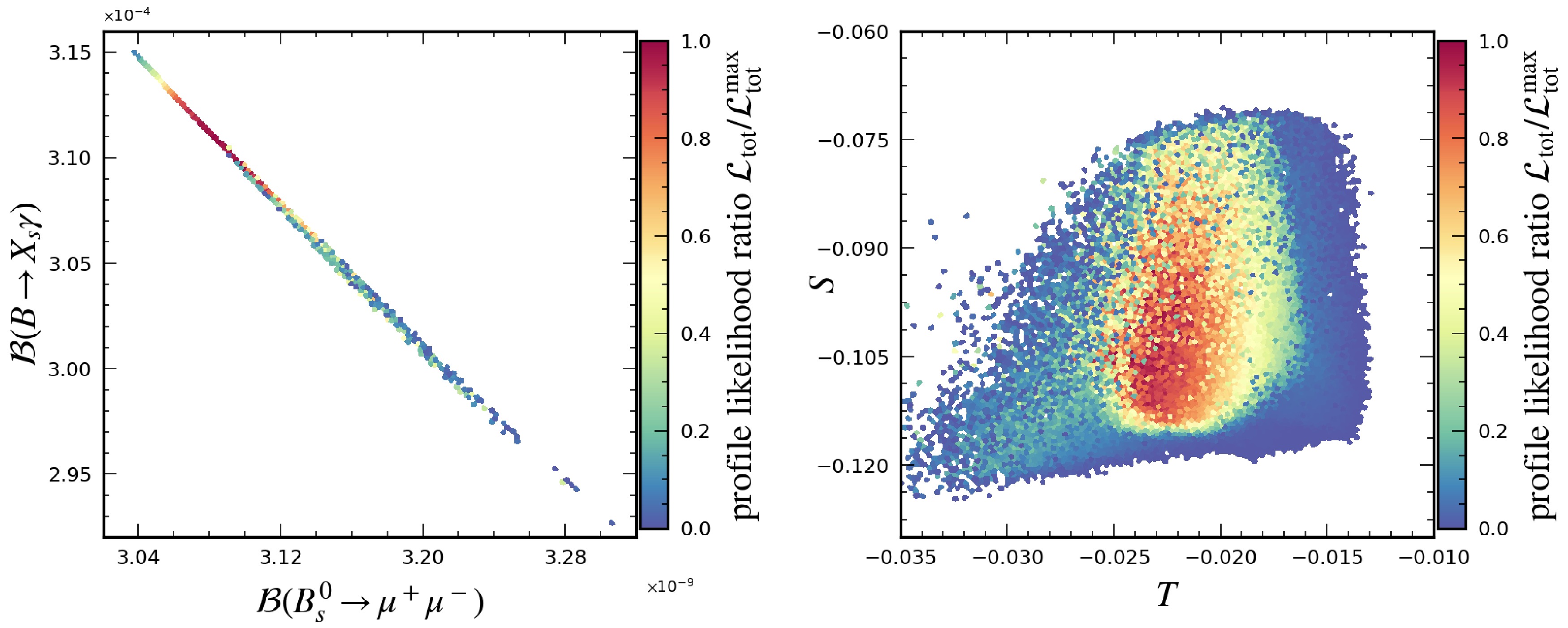

Figure 4.  (color online) Similar to Fig. 1, but shown in the oblique-parameter $ (T, S) $ plane and in the branching-ratio plane for the rare B-meson decays $ B^0_s \to \mu^+ \mu^- $ and $ B \to X_s \gamma $.

The branching ratio scales approximately as $ {\cal{B}}(B \to X_s \gamma) \propto |C_7^{\rm{eff}}|^2 $ [177, 178]. In contrast, the rare decay $ B_s^0 \to \mu^+ \mu^- $ is governed by

where $ {\cal{O}}_{S,P} $ denote scalar and pseudoscalar operators. The corresponding branching ratio depends predominantly on $ |C_{10}|^2 $ in the absence of large scalar contributions [179, 180].

In the GM model, the charged scalars $ H_3^\pm $, $ H_5^\pm $, and $ H_5^{\pm\pm} $ modify both $ C_7 $ and $ C_{10} $ at the one-loop level. However, the loop functions entering $ \Delta C_7 $ and $ \Delta C_{10} $ differ in structure and interfere differently with the SM contributions. For the parameter region relevant to the 95 GeV interpretation, the charged-scalar contribution tends to shift $ C_7 $ and $ C_{10} $ in opposite effective directions relative to their SM values, leading to the nearly linear anti-correlation observed in Fig. 4.

Turning to the EW oblique observables, the T parameter is often regarded as a sensitive probe of custodial symmetry breaking. In the GM model, custodial symmetry is preserved at tree level, so the main contributions to T arise from mass splittings within the triplet and quintuplet states. For all samples, custodial symmetry remains nearly exact, resulting in $ T \approx 0 $. However, for larger $ v_\Delta $ or different values of α, mixing between the light scalar H and the 125 GeV Higgs can shift the masses of certain scalars, inducing mass differences within custodial multiplets and leading to deviations in T.

The S parameter reflects corrections to the Z-boson self-energy and its mixing induced by new-physics states. In the GM model, the S parameter is sensitive to light charged scalars. When the light scalar H has a larger triplet component, such as in the region $ \alpha \sim -\pi/3 $, loop effects are enhanced, resulting in more significant deviations in S. Conversely, when the 125 GeV Higgs boson is near the alignment limit, such as for $ \alpha \sim \pi/3 $ and a small triplet vacuum expectation value $ v_\Delta $, the scalar sector is dominated by the doublet component, and mixing with the triplet states is suppressed. In this regime, the additional custodial-multiplet scalars either become heavier or couple more weakly to the electroweak gauge bosons. As a result, their loop-induced contributions to the gauge-boson self-energies are reduced, leading to smaller corrections to the oblique parameter S.

Finally, Fig. 5 displays the profiled likelihood projected onto the $ (M_{H_5},\,M_{H_3}) $ plane. A compressed spectrum is observed between the custodial fiveplet and triplet masses, with $ \Delta m(m_{H_5}, m_{H_3}) \lt {\cal{O}}(100\; {{\rm{GeV}}}) $. In particular, the mass hierarchy $ M_{H_5}>M_{H_3} $ implies that the doubly charged scalar $ H_5^{\pm\pm} $ tends to decay predominantly into $ H_3^\pm W^\pm $, rather than through the conventional $ W^\pm W^\pm $ mode. As shown in Table 1, the branching ratio $ {\cal{B}}(H_5^{\pm\pm}\to W^\pm W^\pm) $ is typically suppressed to below the ten-percent level, and for the benchmark point $ \mathrm{BP2}$ it can even reach the per-mille level. This feature has important implications for collider phenomenology.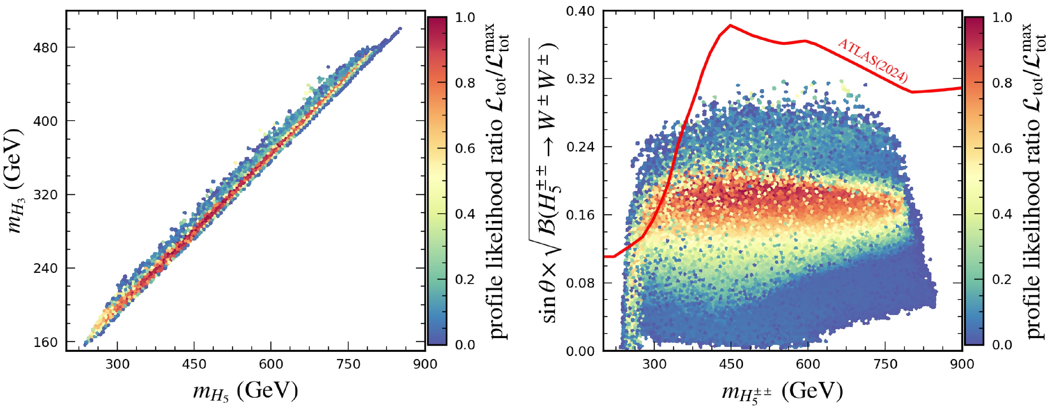

Figure 5.  (color online) Similar to Fig. 1, but showing the $ (m_{H_5}, m_{H_3}) $ panel and the $ m_{H_{5}^{\pm\pm}} $ versus $ \sin\theta_H \times \sqrt{{\cal{B}}\left( H_{5}^{\pm\pm} \to W^\pm W^\pm \right)} $ panel. The red line indicates the limit from the ATLAS search [181] for doubly charged $ H_{5}^{\pm\pm} $ in $ W^\pm W^\pm $ final states.

The right panel of Fig. 5 shows the plane of $ m_{H_5^{\pm\pm}} $ versus $ \sin\theta_H\,\sqrt{{\cal{B}}(H_5^{\pm\pm}\to W^\pm W^\pm)} $, together with the published ATLAS limit [181] derived for the simplified topology with dominant $ H_5^{\pm\pm}\to W^\pm W^\pm $ decays. We emphasize that this comparison is only indicative. In the cascade-dominated regime relevant to our preferred parameter space, the actual signal topology is controlled by $ H_5^{\pm\pm}\to H_3^\pm W^\pm $, and the resulting event kinematics and analysis efficiencies need not coincide with those assumed in the published same-sign diboson search. Therefore, the experimental contour in Fig. 5 should not be interpreted as a strict exclusion bound on the full GM scenario in this region.

Nevertheless, the figure still illustrates an important trend: once the branching ratio into $ W^\pm W^\pm $ is strongly suppressed, the direct sensitivity of existing same-sign diboson searches is correspondingly weakened. A dedicated recast of the relevant ATLAS and CMS analyses, explicitly incorporating the cascade topology $ H_5^{\pm\pm}\to H_3^\pm W^\pm $, would be required to assess the true collider reach for this part of the parameter space.

Additionally, for the Drell–Yan process, which produces $ H_5 $ pairs via γ and Z exchange [182], the production cross section depends only on the gauge coupling and the Higgs mass $ m_{H_5} $, and is independent of $ v_\Delta $, as discussed in the experimental searches. In our work, $ m_{H_5} $ ranges from several hundred GeV, where the cross section is relatively small, making it difficult for current experimental searches to exclude the surviving parameter space. The process $ H_5^{\pm\pm} \to \ell^{\pm}\ell^{\pm} $ proceeds via a lepton-number-violating coupling between the triplet χ and the lepton fields, and was studied at LEP [183]. However, as pointed out in [92], this decay channel becomes comparable to the weak gauge boson decay modes only when $ v_\Delta \lesssim 10^{-4}\; \text{GeV} $, making it negligible in the parameter region of interest for our study.

As discussed in Sec. 4, our main fit uses the $ (\kappa_V,\kappa_F) $ likelihood rather than the full $ \mathrm{HiggsSignals}$ output to avoid double counting Higgs signal-strength information. It is nevertheless useful to verify that the preferred region identified in this reduced Higgs-likelihood treatment remains broadly consistent with the more detailed channel-based evaluation provided by $ \mathrm{HiggsSignals}$. The left panel of Fig. 6 shows the relation between $ \chi^2_\kappa $ and $ \chi^2_{\rm{HS}} $, with the color scale indicating the total profile-likelihood ratio.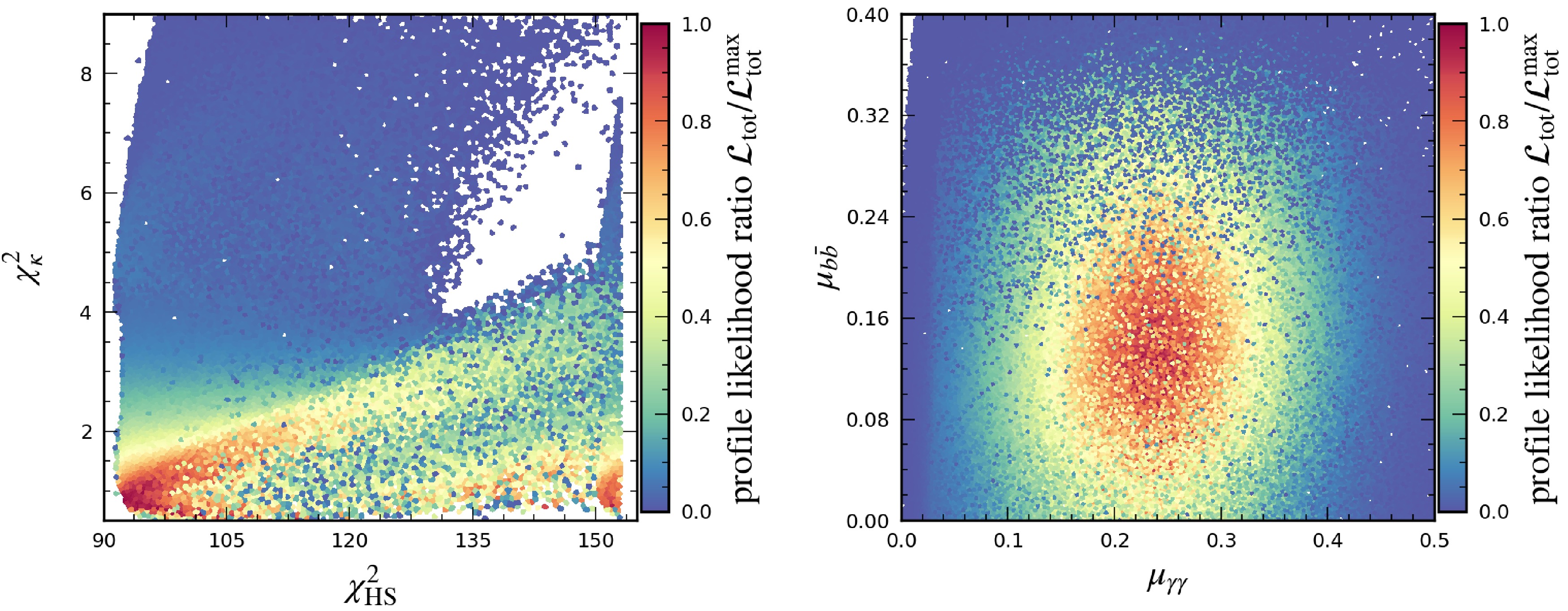

Figure 6.  (color online) Similar to Fig. 1. Left: Relationship between $ \chi^2_\kappa $ and $ \chi^2_{\rm{HS}} $, where $ \chi^2_\kappa $ is derived from the $ (\kappa_V,\kappa_F) $-plane analysis and $ \chi^2_{\rm{HS}} $ is computed using the $ \mathrm{HiggsSignals}$ package. Right: Profile-likelihood distribution projected onto the signal strengths in the $ \gamma\gamma $ and $ b\bar b $ channels.

One can clearly see that parameter points with small $ \chi^2_\kappa $ also tend to yield comparatively small $ \chi^2_{\rm{HS}} $ values. This result demonstrates that the simplified $ (\kappa_V,\kappa_F) $ fit effectively captures the primary Higgs-coupling constraints relevant to our analysis, whereas $ \mathrm{HiggsSignals}$ provides a more comprehensive channel-level evaluation. The spread visible in Fig. 6 indicates that the two approaches are not identical, as expected. In particular, the $ (\kappa_V,\kappa_F) $ fit is based on a compressed description of the 125 GeV Higgs data and therefore does not retain the full channel-by-channel information, production-mode decomposition, or experimental correlations incorporated in $ \mathrm{HiggsSignals}$. For this reason, the κ-plane treatment should be regarded as an effective approximation rather than a complete replacement for the full Higgs likelihood. In practice, it is also somewhat more conservative than the full channel-based $ \mathrm{HiggsSignals}$ evaluation, since the compressed $ (\kappa_V,\kappa_F) $ description retains less experimental information and therefore has weaker discriminating power for excluding parameter points. Nevertheless, this comparison tests the robustness of our results. The conclusion that the $ 95\; {{\rm{GeV}}} $ $ \tau\tau $ signal intensity is constrained by 125 GeV Higgs-boson data holds regardless of whether we use the simplified κ-plane method or the more detailed channel-based evaluation.

The right panel of Fig. 6 shows a related feature of the surviving parameter space in the $ b\bar b $ channel. Although the LEP $ b\bar b $ excess is not included as an input constraint in our fit, some viable parameter points remain compatible with the corresponding preferred signal-strength range. In the GM model, the $ b\bar b $ and $ \tau\tau $ signal strengths are not independent, since both are controlled by the same underlying singlet–doublet mixing structure and share the common factor $ |\kappa_F^H|^2 \cdot \Gamma_h^{\rm{SM}}/\Gamma_H^{\rm{tot}} $, as discussed in Sec. III. As a result, once the preferred region is selected by the combined $ \gamma\gamma $ and $ \tau\tau $ fit, the corresponding prediction for $ \mu_{b\bar b} $ is automatically restricted to a relatively narrow range.

In particular, the best-fit region with $ \mu_{\tau\tau}\sim 0.45 $ tends to predict a $ b\bar b $ signal strength close to the central value of the LEP excess. We do not interpret this as a primary target of the present fit, but rather as a correlated outcome of the surviving region selected by the LHC-driven channels. This behavior can be understood qualitatively from the fact that, unlike the $ \tau\tau $ excess, the $ b\bar b $ signal strength does not face the same direct tension with the precision data of the 125 GeV Higgs boson. Consequently, once the Higgs-coupling constraints compress the viable parameter space, the corresponding prediction in the $ b\bar b $ channel can still remain close to the LEP-preferred range.

Our result should not be viewed as being in conflict with earlier studies, but rather as providing a complementary perspective. Ref. [144] employed a more complete treatment of the Higgs-sector constraints and concluded that the GM model can account for the di-photon excess while remaining compatible with the LEP $ b\bar b $ excess, but cannot reproduce the large central value of the CMS $ \tau\tau $ excess. Ref. [143] further showed that a larger $ \tau\tau $ rate can arise either in a tiny single-peak region or, more efficiently, in a twin-peak setup involving multiple nearly degenerate states. In contrast, our analysis focuses on a single light $\rm CP $-even state and shows that, within this setup, the $ \tau\tau $ signal strength can be raised to a moderate level of order $ 0.5 $, while larger values are constrained by the 125 GeV Higgs data.

In this work, we investigated whether a single light $ CP $-even custodial singlet in the Georgi–Machacek model can jointly accommodate the LHC hints near $ 95\; \mathrm{GeV} $ in the $ \gamma\gamma $ and $ \tau\tau $ channels. The diphoton excess can be accommodated near its central value, whereas $ \mu_{\tau\tau}\simeq0.5 $ lies about $ 1.4\sigma $ below the CMS value of 1.2 and is compatible only at the $ 2\sigma $ level.

The one-loop RG-improved positive-definiteness condition reshapes the allowed parameter space relative to the conventional electroweak-scale BFB requirement and yields a net expansion of the phenomenologically viable region, while remaining consistent with perturbative unitarity, electroweak precision data, B-physics observables, direct searches, and Higgs signal-strength measurements.

The preferred region is characterized by a narrow range of the mixing angle, $ \alpha\simeq-\pi/3 $, a moderate triplet VEV of a few tens of GeV, and a mass hierarchy $ m_{H_3}<m_{H_5} $ at the $ {\cal{O}}(10^2)\; \mathrm{GeV} $ scale. Charged-scalar loops, especially those involving $ H_5^{\pm\pm} $, enhance the diphoton rate, allowing it to approach the experimental central value.

These features make the scenario highly testable. Updated $ \gamma\gamma $ and $ \tau\tau $ searches at the HL-LHC, together with direct probes of the custodial multiplet states, will cover much of the remaining parameter space. Future lepton colliders such as CEPC and FCC-ee will provide decisive tests through precision $ \kappa_V $ measurements.