Radiative generation of chiral vector operators in b → ${{\boldsymbol{sv}}{\overline {\boldsymbol v}}} $ transition

Direct searches for new particles at the LHC have so far yielded null results, placing stringent constraints on physics beyond the Standard Model (SM). In contrast, indirect probes in the flavor sector exhibit persistent tensions, most notably in the flavor-changing neutral current (FCNC) transition $ b \to s \nu \bar{\nu} $. The Belle II collaboration recently reported the first evidence for $ B^+ \to K^+ \nu \bar{\nu} $, with a branching fraction of $ {\cal{B}}_{{\rm{exp}}} = (2.3 \pm 0.7) \times 10^{-5} $ [1], exceeding the SM prediction of $ (4.44 \pm 0.30) \times 10^{-6} $ [2] by $ 2.7\sigma $. This quark-level transition also governs the neutral mode $ B^0 \to K^{*0} \nu \bar{\nu} $, for which the current experimental upper limit of $ 1.8 \times 10^{-5} $ [3] lies roughly a factor of two above the SM expectation of $ (9.47 \pm 1.40) \times 10^{-6} $ [2].

These findings have stimulated a wide range of theoretical interpretations. One class of models postulates the existence of light, invisible states—such as sterile neutrinos [4−13], light dark matter (DM) [14−23], axion-like particles [24−31], or generic long-lived particles [32−38] —which mimic the missing-energy signature of the neutrino pairs. Alternatively, the anomalies can be addressed within the framework of heavy new physics (NP), where virtual exchange of heavy mediators modifies the Wilson coefficients of the low-energy effective Lagrangian [12, 18, 39−56].

These tensions can be further quantified by the ratio $ R \equiv {\cal{B}}(B^0 \to K^{*0} \nu \bar{\nu}) / {\cal{B}}(B^+ \to K^+ \nu \bar{\nu}) $. The experimental upper limit, $ R_{{\rm{exp}}} \le 1.125 $, lies well below the SM prediction $ R_{{\rm{SM}}} = 2.14 \pm 0.35 $. In the framework of low-energy effective theory (LEFT), assuming that the neutrinos remain purely left-handed, scalar and tensor contributions vanish due to chirality constraints. Consequently, the relevant interactions are governed by the vector operators:

Clearly, the tensions cannot be resolved by modifying only the left-handed operator $ {\cal{O}}_V^L $, as such a modification would rescale both rates identically, leaving the ratio invariant. Thus, the presence of the right-handed operator $ {\cal{O}}_V^R $ is a necessary ingredient for any explanation involving these vector currents [41, 44].

As highlighted in Ref. [41], addressing the deviation in R at tree level typically requires non-minimal field content, such as the introduction of at least three distinct leptoquarks, whereas loop-level solutions have broadly been considered challenging. Nonetheless, the radiative generation of $ {\cal{O}}_V^{L} $ and $ {\cal{O}}_V^{R} $ provides a well-motivated model-building paradigm. Historically, loop-induced frameworks have offered economical pathways to unify disparate phenomenological puzzles—such as neutrino masses, dark matter, and other flavor anomalies—by linking them through a shared internal sector. Furthermore, loop-induced processes naturally provide a suppression mechanism. Should future, higher-statistics experimental updates from Belle II shift the central values and reduce the size of the anomaly, a radiatively generated contribution would naturally accommodate a smaller residual deviation without necessitating tiny tree-level couplings. Beyond these phenomenological considerations, systematically generating both left- and right-handed vector operators via loop processes represents a non-trivial structural feature of effective field theory. However, a comprehensive classification of such models has not yet been systematically explored.

Motivated by these considerations, we employ a diagrammatic method to generate the complete set of one-loop topologies involving new scalars and fermions. We classify the minimal ultraviolet (UV) extensions capable of simultaneously generating both $ {\cal{O}}_V^L $ and $ {\cal{O}}_V^R $. To systematically navigate the multidimensional parameter space and explore how different coupling degeneracies govern the interference patterns in the decay rates, we define four representative flavor structures for the quark sector. By analyzing these specific arrangements, we quantitatively determine the maximum reach of these radiative contributions while ensuring compatibility with complementary flavor observables.

The remainder of this paper is organized as follows. In Sec. II, we present the systematic classification of one-loop topologies and identify the UV extensions capable of generating the required effective operators. Based on this classification, we select two minimal benchmark models for phenomenological study: one combines diagrams that independently generate $ {\cal{O}}_V^R $ and $ {\cal{O}}_V^L $; the other employs a single topology that produces both chiralities. Section III details these models. In Sec. IV, we define the relevant observables and establish the constraints on the Wilson coefficients imposed by experimental data. The phenomenological analysis of these models is presented in Sec. V. Finally, we summarize our findings in Sec. VI, with technical details provided in the Appendices.

In this work, we focus primarily on the radiative generation of the relevant effective operators. To systematically isolate and evaluate these loop-level effects, our phenomenological analysis proceeds under the working assumption that they constitute the dominant new-physics contribution. This condition can be naturally realized in various models through the imposition of a discrete or flavor symmetry, analogous to established models of radiative neutrino mass generation (see, e.g., Refs. [57−59]). Because the introduction of such symmetries is a standard technique in model building, we assume that a suitable symmetry can always be implemented to forbid the tree-level contributions. Consequently, we do not specify the exact symmetry structure in each case; instead, we focus on the general classification of all viable one-loop model structures.

Our classification scheme is based on a hierarchy of concepts [58], which we define as follows:

● Topology: We define a topology as the underlying graphical structure of a Feynman diagram, abstracted from the physical properties of the particles involved. It is determined solely by its vertices and their connectivity, without regard to the Lorentz nature or quantum numbers of the fields.

● Renormalizable Topology: A topology is deemed renormalizable if it can be constructed exclusively from vertices corresponding to interactions with mass dimension less than or equal to four. This ensures that the corresponding operator can be embedded in a renormalizable quantum field theory.

● Diagram: We refer to a topology as a diagram once a specific particle type (i.e., scalar, vector, or fermion) has been assigned to each line.

● Model-Diagram: A model-diagram is a fully specified diagram in which all internal fields are assigned a complete set of quantum numbers under the relevant symmetries (e.g., representations of the SM gauge group).

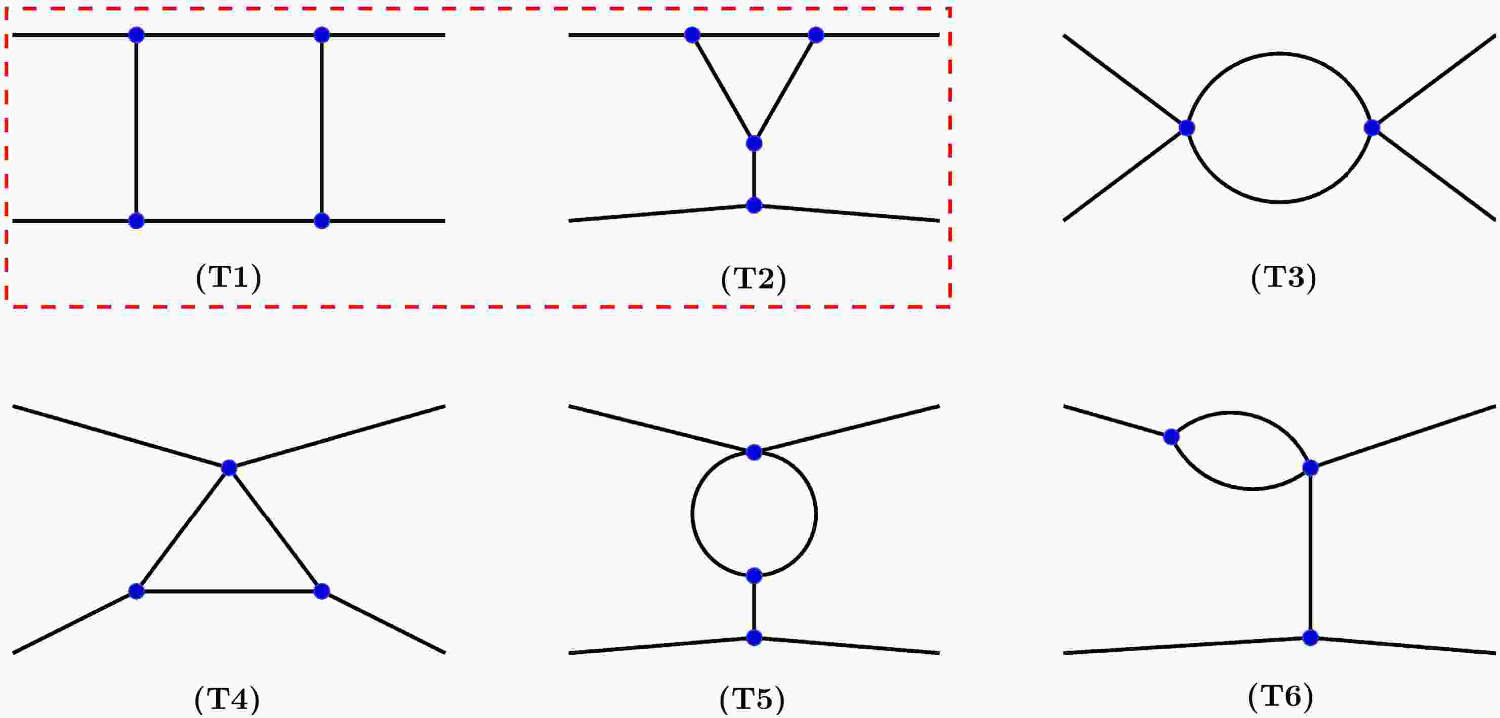
We begin our classification by systematically generating all one-loop topologies for a four-point interaction using only three- and four-point vertices. From this initial set, we discard all graphs corresponding to tadpoles or external-line self-energy corrections, since they lead to divergent loop integrals. This leaves six topologies, which we depict in Fig. 1.

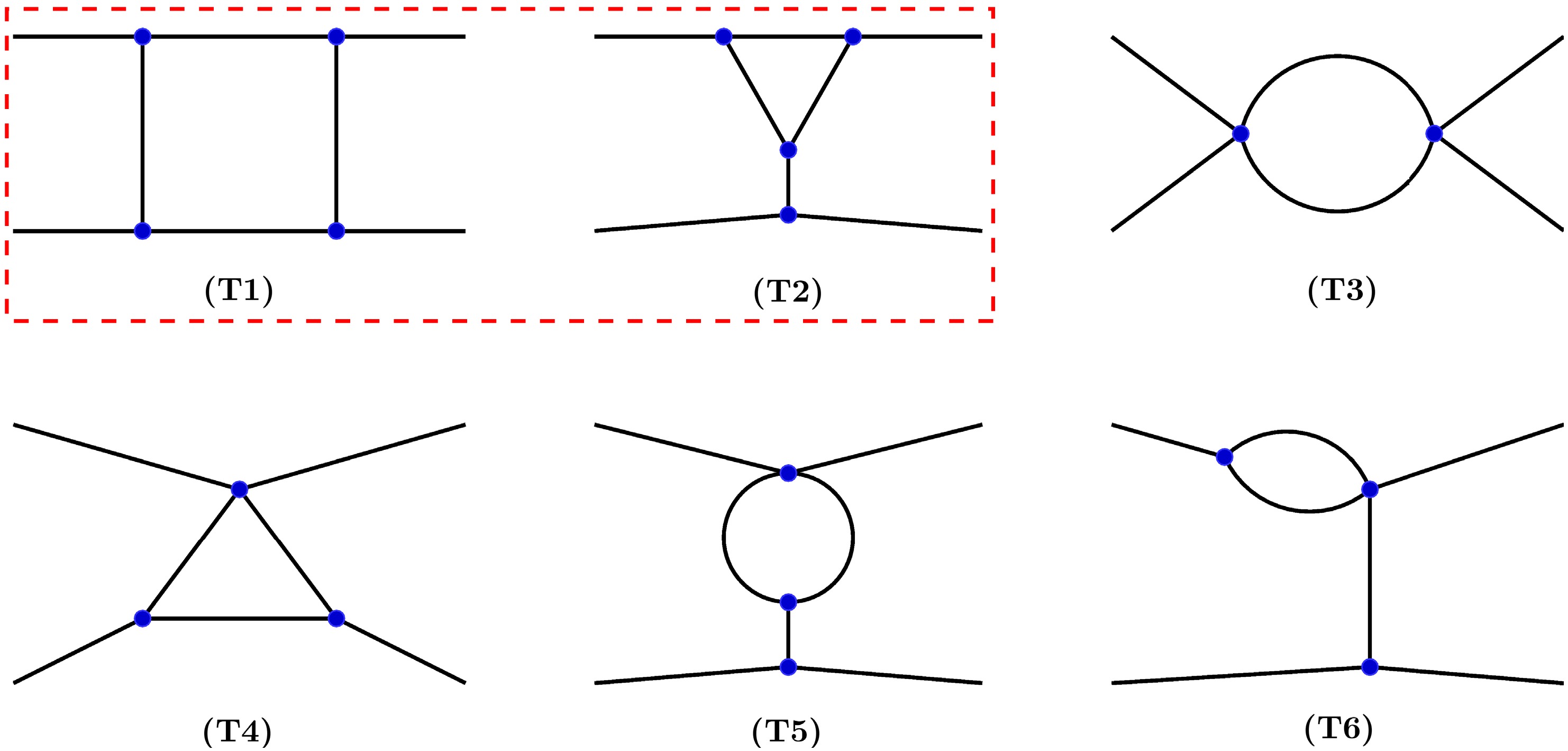
Figure 1.  (color online) One-loop topologies with three- and four-point vertices and four external legs. Topologies T1 and T2, highlighted in the red-dashed box, are renormalizable.

We categorize these six topologies according to the definitions established previously. The first class, comprising T1 and T2, consists exclusively of three-point vertices and is therefore classified as renormalizable. In contrast, the remaining topologies—T3, T4, T5, and T6—each contain at least one four-point vertex. Since all external lines in our operators are fermionic, any such four-point vertex necessarily corresponds to an operator of mass dimension greater than four. Consequently, these four topologies are classified as non-renormalizable and will not be considered further in this work.

We now proceed to construct the diagrams for the renormalizable topologies T1 and T2. By assigning fermion and scalar identities to the internal lines while keeping the four external lines as fermions, we obtain the three distinct diagrams shown in Fig. 2. In our convention, solid lines denote fermions and dashed lines denote scalars. These diagrams are distinguished by their structure, which we categorize as either reducible or irreducible. Here, we define a one-loop diagram as reducible if it functions as a radiative correction to a renormalizable vertex. Accordingly, diagram T1-1 is an irreducible box diagram, whereas T2-1 and T2-2 are reducible, each containing a one-loop vertex correction highlighted in red.

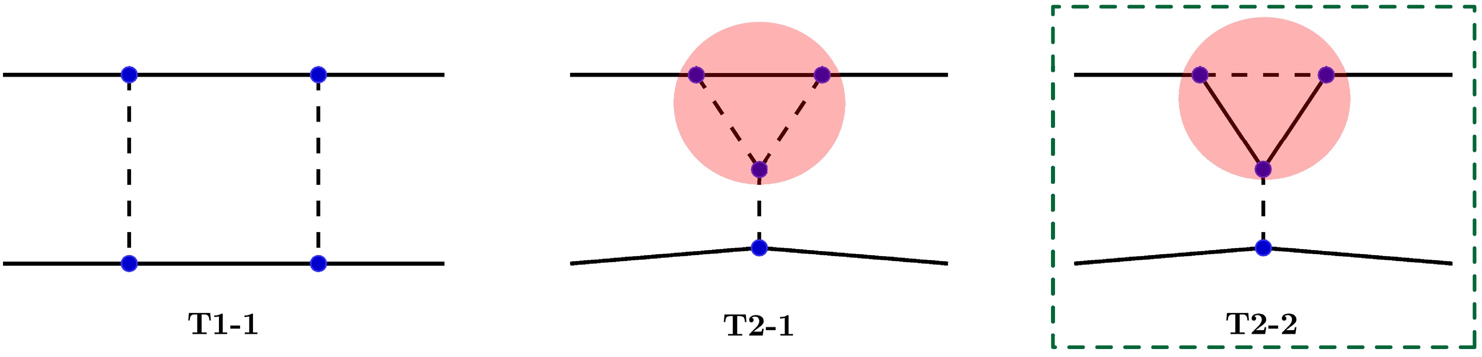
Figure 2.  (color online) Possible one-loop diagrams for the topologies T1 and T2, where dashed lines denote scalars and solid lines denote fermions. All T2 diagrams contain a reducible three-point loop vertex, highlighted in red. The T2-2 diagram, enclosed in the green dashed box, has an ultraviolet-divergent loop integral.

This structural distinction has a critical physical implication. The presence of a reducible vertex correction, as seen in T2-1 and T2-2, generically implies the existence of a corresponding tree-level diagram that contributes to the same four-point operator. To ensure that the one-loop contribution is dominant without fine-tuning or the imposition of special symmetries to forbid the tree-level term, such diagrams must be set aside. Furthermore, the loop integral in diagram T2-2 (enclosed in the green-dashed box) is UV divergent. For these reasons, we will focus our subsequent analysis on the irreducible T1-1 diagram, which represents a genuine one-loop realization [57, 58]. We note, however, that diagram T2-1 remains a viable candidate in models where a symmetry is imposed to forbid its tree-level contribution (e.g., under a $ Z_2 $ symmetry where the SM fields and the NP mediator connecting the two external lines are $ Z_2 $-even, while the three NP fields running in the loop are $ Z_2 $-odd).

With the T1-1 diagram established as our template, the next step is to construct its concrete physical realizations. We assign specific particle content to the internal lines: two vector-like fermions ($ \Psi_1, \Psi_3 $) and two scalars ($ X_2, X_4 $). We then attach the external fields—a b quark, an s quark, and two neutrinos (ν)—in all non-equivalent configurations, leaving their chirality unspecified at this stage. This procedure yields the six unique diagrams depicted in Fig. 3. For notational simplicity, we drop the "T1-1" prefix and henceforth refer to these diagrams by their labels, (a) through (f).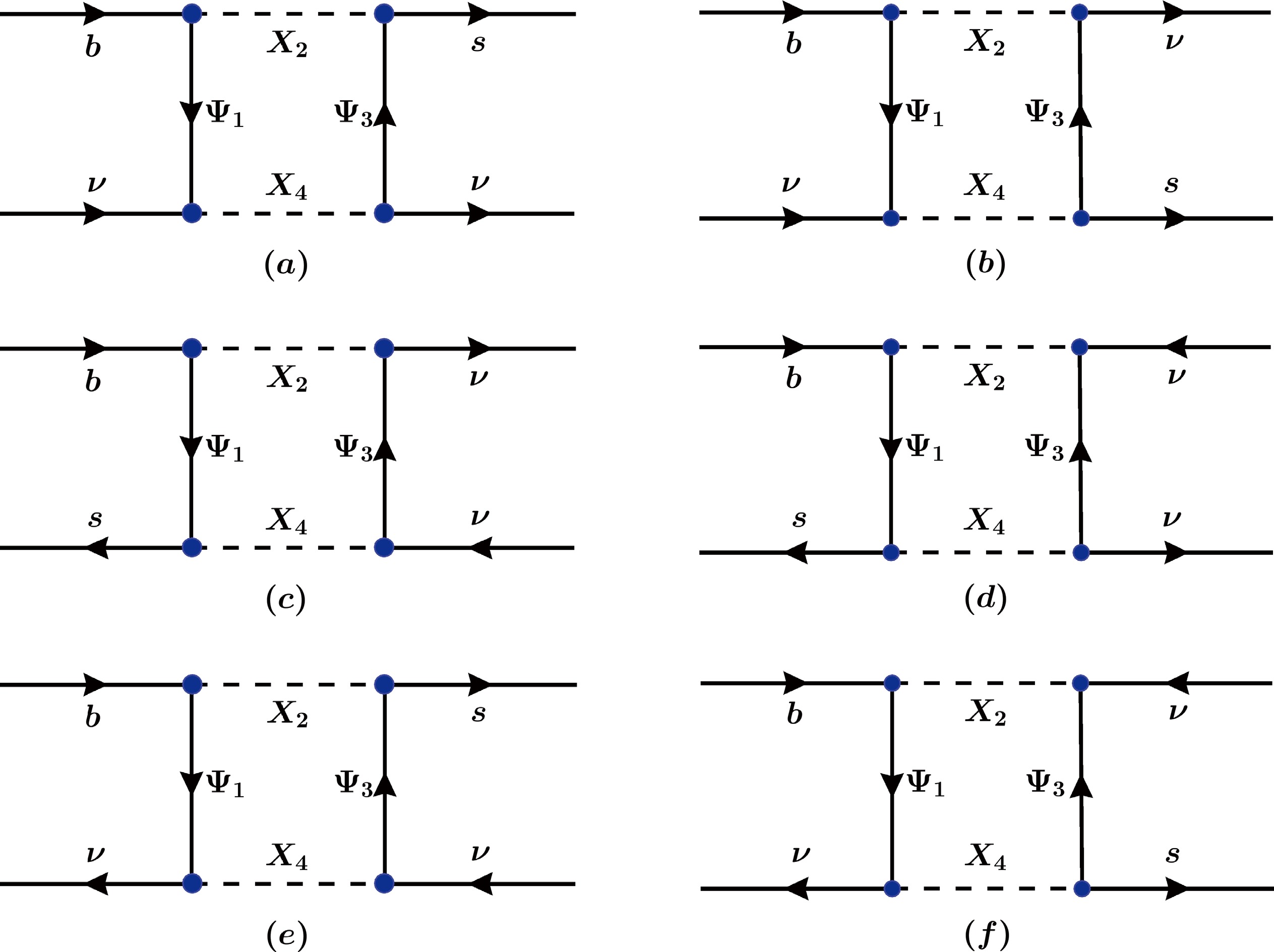

Figure 3.  The six distinct diagrams obtained from the T1-1 diagram by permuting the external fields $ (b, s, \nu, \nu) $. The internal fields are fixed as fermions $ (\Psi_1, \Psi_3) $ and scalars $ (X_2, X_4) $.

In principle, the T1-1 topology can accommodate SM particles (such as SM fermions and electroweak gauge bosons) as well as exotic vector mediators. Here, we restrict all internal propagators to beyond-the-SM states, leaving open the possibility that these mediators belong to a dark or hidden sector. We focus exclusively on new scalars and fermions, omitting new vector bosons, since their inclusion would typically require an extended gauge symmetry and an associated symmetry-breaking sector, introducing additional model-dependent constraints beyond our minimal setup. Finally, we take the new fermions to be vector-like under $ {\rm{SU}}(3)_c \times {\rm{SU}}(2)_L \times {\rm{U}}(1)_Y $, which automatically preserves gauge-anomaly cancellation in the SM.

We now promote the diagrams to model-diagrams by assigning SM quantum numbers to the internal fields, requiring conservation of SM gauge symmetry at each vertex. The quantum numbers of the external fields provide the necessary boundary conditions, fixed by the choice of target operator ($ {\cal{O}}_V^{R} $ or $ {\cal{O}}_V^{L} $). For operators involving SU(2)_L charges, we treat the external left-handed fermions as components of their respective doublets: the b and s quarks as part of the quark doublet Q, and the neutrino as part of the lepton doublet L. The nature of the constraints on the internal fields then depends on the gauge group. For U(1)_Y, the additive nature of hypercharge means that a choice for one internal field's hypercharge fixes all others. For SU(3)_c and SU(2)_L, however, the tensor product of representations decomposes into multiple irreducible representations, allowing greater flexibility. In this work, to ensure a tractable classification, we restrict our analysis to color singlets and triplets for SU(3)_c, and to SU(2)_L representations up to triplets.

As a representative example, Table 1 presents the complete set of allowed SM quantum-number assignments for the internal fields of diagram (c) that generate the operator $ {\cal{O}}^L_V $. The analogous results for the remaining five diagrams are compiled in Appendix C. The table is organized into three sections, listing the viable assignments for the SU(3)_c and SU(2)_L representations, and the corresponding U(1)_Y hypercharges. Each physical model is constructed by selecting one complete set of SU(3)_c representations (e.g., case A) and one set of SU(2)_L representations (e.g., case I). The hypercharges are not independent; as shown in the final section, they are all uniquely determined by the choice of a single free parameter, α, which we define as the hypercharge of the fermion $ \Psi_1 $ ($ \alpha \equiv Y_{\Psi_1} $).

A crucial aspect of this analysis is the matching procedure between the high-scale UV model and the low-energy effective operators. When integrating out the heavy internal fields, the UV model does not directly generate the LEFT operators $ {\cal{O}}^{L,R}_V $. Instead, at the new physics scale Λ, it must first be matched onto the appropriate set of dimension-six operators in the Standard Model Effective Field Theory (SMEFT). For the processes we consider, the relevant SMEFT Lagrangian is

where the operators are defined as

with $ \tau^I $ being the Pauli matrices and $ p, r, s, t $ the generation indices. In our calculation, we adopt two primary conventions. First, the new physics scale Λ is absorbed into the definition of the Wilson coefficients. Second, we work in the "down basis," in which the down-type quark and charged-lepton Yukawa matrices are diagonal. In this framework, the SMEFT operators must be evolved through renormalization group (RG) running from the high scale to the electroweak scale, where they can be matched onto the LEFT operator basis, which includes $ {\cal{O}}^L_V $ and $ {\cal{O}}^R_V $ [60].

To illustrate this procedure, we perform an explicit calculation for a representative case: model A-V, constructed from diagram (c) using the SU(3)_c and SU(2)_L assignments from cases A and V in Table 1, respectively. For simplicity, we assume that the scalars $ X_2 $ and $ X_4 $ are the same particle, since they share the same SM quantum numbers. The interaction Lagrangian for this model is given by

where in the second line we have made the SU(2)_L structure explicit. The Greek letters ($ \alpha, \beta, \cdots $) denote SU(2)_L indices in the fundamental representation, taking values 1 and 2, while the color indices are suppressed because of the trivial SU(3)_c structure of this model. The symbols $ g_{1,2} $ denote the coupling constants, and the SU(2)_L tensor ξ is defined as $ \xi^A=((1+\tau^3)/2, \tau^1/\sqrt{2},(1-\tau^3)/2) $ with $ A\in 1,2,3 $.

Integrating out the heavy fields $ \Psi_i $ and $ X_2 $ at one loop yields the following effective four-fermion operator:

where $ J_4 $ is the loop function defined in Appendix A. The final step is to evaluate the product of the SU(2)_L tensors in Eq. (5). This algebraic simplification maps the operator directly onto a specific linear combination of the SMEFT operators $ Q^{(1)}_{\ell q} $ and $ Q^{(3)}_{\ell q} $. The resulting effective Lagrangian at the scale Λ is therefore

The Wilson coefficients of the SMEFT operators are therefore determined by the couplings and masses of the UV model. For ease of future reference, we list the coefficients of $ Q^{(1)}_{\ell q} $ and $ Q^{(3)}_{\ell q} $ for all valid models in Table 2.

Two key features characterize this classification. First, certain gauge-invariant assignments are phenomenologically trivial. For instance, the $ SU(2)_L $ assignment $ (\Psi_1, X_2, \Psi_3, X_4) \to (1, 2, 1, 2) $ generates an $ SU(2)_L $ structure of the form

Following electroweak symmetry breaking, the tree-level matching of this specific operator combination onto the target $ {\cal{O}}^L_V $ vanishes. Consequently, we exclude solutions that yield this null result from our final analysis, as shown in Table 2 and Appendix C.

Second, in models with complex mediators (i.e., Dirac fermions and complex scalars), a correspondence emerges between diagram topology and operator chirality. In this scenario, diagrams (c) and (d) can generate both $ {\cal{O}}^L_V $ and $ {\cal{O}}^R_V $, whereas diagrams (a) and (b) are restricted to $ {\cal{O}}^R_V $, and (e) and (f) are limited to $ {\cal{O}}^L_V $. This chiral distinction is relaxed in the presence of real fields, such as Majorana fermions or real scalars, which introduce new interaction structures that allow previously restricted diagrams to generate both chiralities. These effects are explicitly demonstrated by our benchmark models in Sec. III.

In this work, we focus primarily on the radiative generation of the relevant effective operators. To systematically isolate and evaluate these loop-level effects, our phenomenological analysis proceeds under the working assumption that they constitute the dominant new-physics contribution. This condition can be naturally realized in various models through the imposition of a discrete or flavor symmetry, analogous to established models of radiative neutrino mass generation (see, e.g., Refs. [57−59]). Because the introduction of such symmetries is a standard technique in model building, we assume that a suitable symmetry can always be implemented to forbid the tree-level contributions. Consequently, we do not specify the exact symmetry structure in each case; instead, we focus on the general classification of all viable one-loop model structures.

Our classification scheme is based on a hierarchy of concepts [58], which we define as follows:

● Topology: We define a topology as the underlying graphical structure of a Feynman diagram, abstracted from the physical properties of the particles involved. It is determined solely by its vertices and their connectivity, without regard to the Lorentz nature or quantum numbers of the fields.

● Renormalizable Topology: A topology is deemed renormalizable if it can be constructed exclusively from vertices corresponding to interactions with mass dimension less than or equal to four. This ensures that the corresponding operator can be embedded in a renormalizable quantum field theory.

● Diagram: We refer to a topology as a diagram once a specific particle type (i.e., scalar, vector, or fermion) has been assigned to each line.

● Model-Diagram: A model-diagram is a fully specified diagram in which all internal fields are assigned a complete set of quantum numbers under the relevant symmetries (e.g., representations of the SM gauge group).

We begin our classification by systematically generating all one-loop topologies for a four-point interaction using only three- and four-point vertices. From this initial set, we discard all graphs corresponding to tadpoles or external-line self-energy corrections, since they lead to divergent loop integrals. This leaves six topologies, which we depict in Fig. 1.

Figure 1.  (color online) One-loop topologies with three- and four-point vertices and four external legs. Topologies T1 and T2, highlighted in the red-dashed box, are renormalizable.

We categorize these six topologies according to the definitions established previously. The first class, comprising T1 and T2, consists exclusively of three-point vertices and is therefore classified as renormalizable. In contrast, the remaining topologies—T3, T4, T5, and T6—each contain at least one four-point vertex. Since all external lines in our operators are fermionic, any such four-point vertex necessarily corresponds to an operator of mass dimension greater than four. Consequently, these four topologies are classified as non-renormalizable and will not be considered further in this work.

We now proceed to construct the diagrams for the renormalizable topologies T1 and T2. By assigning fermion and scalar identities to the internal lines while keeping the four external lines as fermions, we obtain the three distinct diagrams shown in Fig. 2. In our convention, solid lines denote fermions and dashed lines denote scalars. These diagrams are distinguished by their structure, which we categorize as either reducible or irreducible. Here, we define a one-loop diagram as reducible if it functions as a radiative correction to a renormalizable vertex. Accordingly, diagram T1-1 is an irreducible box diagram, whereas T2-1 and T2-2 are reducible, each containing a one-loop vertex correction highlighted in red.

Figure 2.  (color online) Possible one-loop diagrams for the topologies T1 and T2, where dashed lines denote scalars and solid lines denote fermions. All T2 diagrams contain a reducible three-point loop vertex, highlighted in red. The T2-2 diagram, enclosed in the green dashed box, has an ultraviolet-divergent loop integral.

This structural distinction has a critical physical implication. The presence of a reducible vertex correction, as seen in T2-1 and T2-2, generically implies the existence of a corresponding tree-level diagram that contributes to the same four-point operator. To ensure that the one-loop contribution is dominant without fine-tuning or the imposition of special symmetries to forbid the tree-level term, such diagrams must be set aside. Furthermore, the loop integral in diagram T2-2 (enclosed in the green-dashed box) is UV divergent. For these reasons, we will focus our subsequent analysis on the irreducible T1-1 diagram, which represents a genuine one-loop realization [57, 58]. We note, however, that diagram T2-1 remains a viable candidate in models where a symmetry is imposed to forbid its tree-level contribution (e.g., under a $ Z_2 $ symmetry where the SM fields and the NP mediator connecting the two external lines are $ Z_2 $-even, while the three NP fields running in the loop are $ Z_2 $-odd).

With the T1-1 diagram established as our template, the next step is to construct its concrete physical realizations. We assign specific particle content to the internal lines: two vector-like fermions ($ \Psi_1, \Psi_3 $) and two scalars ($ X_2, X_4 $). We then attach the external fields—a b quark, an s quark, and two neutrinos (ν)—in all non-equivalent configurations, leaving their chirality unspecified at this stage. This procedure yields the six unique diagrams depicted in Fig. 3. For notational simplicity, we drop the "T1-1" prefix and henceforth refer to these diagrams by their labels, (a) through (f).

Figure 3.  The six distinct diagrams obtained from the T1-1 diagram by permuting the external fields $ (b, s, \nu, \nu) $. The internal fields are fixed as fermions $ (\Psi_1, \Psi_3) $ and scalars $ (X_2, X_4) $.

In principle, the T1-1 topology can accommodate SM particles (such as SM fermions and electroweak gauge bosons) as well as exotic vector mediators. Here, we restrict all internal propagators to beyond-the-SM states, leaving open the possibility that these mediators belong to a dark or hidden sector. We focus exclusively on new scalars and fermions, omitting new vector bosons, since their inclusion would typically require an extended gauge symmetry and an associated symmetry-breaking sector, introducing additional model-dependent constraints beyond our minimal setup. Finally, we take the new fermions to be vector-like under $ {\rm{SU}}(3)_c \times {\rm{SU}}(2)_L \times {\rm{U}}(1)_Y $, which automatically preserves gauge-anomaly cancellation in the SM.

We now promote the diagrams to model-diagrams by assigning SM quantum numbers to the internal fields, requiring conservation of SM gauge symmetry at each vertex. The quantum numbers of the external fields provide the necessary boundary conditions, fixed by the choice of target operator ($ {\cal{O}}_V^{R} $ or $ {\cal{O}}_V^{L} $). For operators involving SU(2)_L charges, we treat the external left-handed fermions as components of their respective doublets: the b and s quarks as part of the quark doublet Q, and the neutrino as part of the lepton doublet L. The nature of the constraints on the internal fields then depends on the gauge group. For U(1)_Y, the additive nature of hypercharge means that a choice for one internal field's hypercharge fixes all others. For SU(3)_c and SU(2)_L, however, the tensor product of representations decomposes into multiple irreducible representations, allowing greater flexibility. In this work, to ensure a tractable classification, we restrict our analysis to color singlets and triplets for SU(3)_c, and to SU(2)_L representations up to triplets.

As a representative example, Table 1 presents the complete set of allowed SM quantum-number assignments for the internal fields of diagram (c) that generate the operator $ {\cal{O}}^L_V $. The analogous results for the remaining five diagrams are compiled in Appendix C. The table is organized into three sections, listing the viable assignments for the SU(3)_c and SU(2)_L representations, and the corresponding U(1)_Y hypercharges. Each physical model is constructed by selecting one complete set of SU(3)_c representations (e.g., case A) and one set of SU(2)_L representations (e.g., case I). The hypercharges are not independent; as shown in the final section, they are all uniquely determined by the choice of a single free parameter, α, which we define as the hypercharge of the fermion $ \Psi_1 $ ($ \alpha \equiv Y_{\Psi_1} $).

A crucial aspect of this analysis is the matching procedure between the high-scale UV model and the low-energy effective operators. When integrating out the heavy internal fields, the UV model does not directly generate the LEFT operators $ {\cal{O}}^{L,R}_V $. Instead, at the new physics scale Λ, it must first be matched onto the appropriate set of dimension-six operators in the Standard Model Effective Field Theory (SMEFT). For the processes we consider, the relevant SMEFT Lagrangian is

where the operators are defined as

with $ \tau^I $ being the Pauli matrices and $ p, r, s, t $ the generation indices. In our calculation, we adopt two primary conventions. First, the new physics scale Λ is absorbed into the definition of the Wilson coefficients. Second, we work in the "down basis," in which the down-type quark and charged-lepton Yukawa matrices are diagonal. In this framework, the SMEFT operators must be evolved through renormalization group (RG) running from the high scale to the electroweak scale, where they can be matched onto the LEFT operator basis, which includes $ {\cal{O}}^L_V $ and $ {\cal{O}}^R_V $ [60].

To illustrate this procedure, we perform an explicit calculation for a representative case: model A-V, constructed from diagram (c) using the SU(3)_c and SU(2)_L assignments from cases A and V in Table 1, respectively. For simplicity, we assume that the scalars $ X_2 $ and $ X_4 $ are the same particle, since they share the same SM quantum numbers. The interaction Lagrangian for this model is given by

where in the second line we have made the SU(2)_L structure explicit. The Greek letters ($ \alpha, \beta, \cdots $) denote SU(2)_L indices in the fundamental representation, taking values 1 and 2, while the color indices are suppressed because of the trivial SU(3)_c structure of this model. The symbols $ g_{1,2} $ denote the coupling constants, and the SU(2)_L tensor ξ is defined as $ \xi^A=((1+\tau^3)/2, \tau^1/\sqrt{2},(1-\tau^3)/2) $ with $ A\in 1,2,3 $.

Integrating out the heavy fields $ \Psi_i $ and $ X_2 $ at one loop yields the following effective four-fermion operator:

where $ J_4 $ is the loop function defined in Appendix A. The final step is to evaluate the product of the SU(2)_L tensors in Eq. (5). This algebraic simplification maps the operator directly onto a specific linear combination of the SMEFT operators $ Q^{(1)}_{\ell q} $ and $ Q^{(3)}_{\ell q} $. The resulting effective Lagrangian at the scale Λ is therefore

The Wilson coefficients of the SMEFT operators are therefore determined by the couplings and masses of the UV model. For ease of future reference, we list the coefficients of $ Q^{(1)}_{\ell q} $ and $ Q^{(3)}_{\ell q} $ for all valid models in Table 2.

Two key features characterize this classification. First, certain gauge-invariant assignments are phenomenologically trivial. For instance, the $ SU(2)_L $ assignment $ (\Psi_1, X_2, \Psi_3, X_4) \to (1, 2, 1, 2) $ generates an $ SU(2)_L $ structure of the form

Following electroweak symmetry breaking, the tree-level matching of this specific operator combination onto the target $ {\cal{O}}^L_V $ vanishes. Consequently, we exclude solutions that yield this null result from our final analysis, as shown in Table 2 and Appendix C.

Second, in models with complex mediators (i.e., Dirac fermions and complex scalars), a correspondence emerges between diagram topology and operator chirality. In this scenario, diagrams (c) and (d) can generate both $ {\cal{O}}^L_V $ and $ {\cal{O}}^R_V $, whereas diagrams (a) and (b) are restricted to $ {\cal{O}}^R_V $, and (e) and (f) are limited to $ {\cal{O}}^L_V $. This chiral distinction is relaxed in the presence of real fields, such as Majorana fermions or real scalars, which introduce new interaction structures that allow previously restricted diagrams to generate both chiralities. These effects are explicitly demonstrated by our benchmark models in Sec. III.

As established in Sec. I, a viable explanation for the observed ratio $ {\cal{B}}(B^0\to K^{*0}\nu\bar{\nu})/{\cal{B}}(B^+\to K^{+}\nu\bar{\nu}) $, which deviates from the SM prediction, requires the simultaneous generation of both $ {\cal{O}}^L_V $ and $ {\cal{O}}^R_V $. Our classification in Sec. II provides a clear route to achieving this. We showed that diagrams (c) and (d) can each independently generate both operator chiralities, whereas diagrams (a)/(b) and (e)/(f) form complementary pairs that generate $ {\cal{O}}^R_V $ and $ {\cal{O}}^L_V $, respectively. Although a simple combination of any two such viable models could suffice, this approach is often unattractive because it introduces a large number of new particles. We therefore impose an additional criterion of minimality and seek the most parsimonious models capable of accomplishing this task.

By systematically surveying all valid model combinations, we have identified two particularly economical scenarios. The most minimal model, containing only four new fields, arises from combining two distinct solutions derived from diagram (c). A second competitive scenario, containing five new fields, can be constructed by combining a model from diagram (a) with one from diagram (e). All other combinations result in models with six or more new degrees of freedom and are therefore not considered further in this work.

Based on this analysis, we select two benchmark models for detailed study; their particle content and SM gauge representations are given in Table 3. The first, which we term the "scalar-rich model", is notable for its predominantly scalar content. Interestingly, for the specific hypercharge assignment $ \alpha=0 $, the states $ S_1 $ and $ S_3 $ in this model correspond precisely to the two scalar leptoquarks introduced in Ref. [41] to address the anomalies via tree-level exchanges. The second, termed the "fermion-rich model", is instead dominated by new fermionic degrees of freedom.

We first consider the scalar-rich model. This benchmark is constructed by combining diagram (a), which generates $ {\cal{O}}^R_V $, with diagram (e), which generates $ {\cal{O}}^L_V $. To obtain a minimal realization, we identify the internal fermion in both diagrams as a single field, Ψ, while treating the four scalars as distinct fields, relabeled $ S_{1, \cdots, 4} $. The relevant interaction Lagrangian is

where i is a generation index, $ L^c_i $ denotes the charge-conjugated lepton doublet $ L_i $, and $ \alpha, \beta $ are $ S U(2)_L $ indices contracted either trivially (diagonally) or through the totally antisymmetric tensor $ \epsilon_{\alpha\beta} $.

This model exhibits a special feature when the hypercharge parameter $ \alpha=0 $, in which case Ψ can be a Majorana fermion. This possibility gives rise to new "crossed" diagrams. As shown in Fig. 4, crossing the internal fermion lines of diagram (a) produces a new diagram ($ a^\prime $), which is topologically identical to diagram (e). Similarly, the crossed version of diagram (e) is topologically equivalent to diagram (a). Consequently, the Majorana nature of Ψ provides an additional mechanism for generating the required operators from the same fundamental Lagrangian.

Figure 4.  (color online) Illustration of the new diagrammatic contribution that arises in the scalar-rich model when the mediating Ψ is a Majorana particle. The box diagram (a) is then accompanied by a "crossed" diagram, denoted ($ a^\prime $), in which the internal fermion lines are exchanged. Note that this crossed diagram is topologically equivalent to diagram (e).

Integrating out the new degrees of freedom yields the effective Lagrangian,

with the Wilson coefficients given by

Here, the factor $ \eta^M=1 $ parameterizes the additional contributions from a Majorana fermion Ψ; for $ \eta^M=0 $, these contributions are absent. The quantity $ I_4 $ denotes the corresponding new loop function, defined in Appendix A.

We now turn to the fermion-rich model, which is constructed by combining two distinct solutions from diagram (c) to generate both $ {\cal{O}}^L_V $ and $ {\cal{O}}^R_V $. To realize this minimal spectrum, we postulate that the internal scalar is a single field, S, shared by both solutions, and that one of the internal fermions is likewise common to both, which we denote by $ \Psi_2 $. The remaining two fermions are distinct fields, denoted by $ \Psi_1 $ and $ \Psi_3 $. This particular field content leads to the following interaction Lagrangian:

where i denotes the generation index and α is the $ S U(2)_L $ index.

As in the scalar-rich case, if the scalar S is a real field (i.e., $ \alpha=-1/3 $), "crossed-scalar" diagrams can also contribute. As illustrated in Fig. 5, box diagram (c) is accompanied by a crossed diagram ($ c^\prime $), in which the internal scalar lines are exchanged. This new diagram ($ c^\prime $) can be topologically rearranged to demonstrate its equivalence to diagram (d), via the intermediate form ($ c^{\prime\prime} $).

Figure 5.  (color online)Illustration of additional diagrammatic contributions in the fermion-rich model that arise when the scalar mediator S is a real field. The box diagram (c) is accompanied by a "crossed-scalar" diagram ($ c^\prime $). This crossed diagram can be topologically rearranged to demonstrate its equivalence to diagram ($ c^{\prime\prime} $), which is itself identical to the box diagram (d).

Integrating out the new particles in the fermion-rich model yields the same operator structure as in Eq. (9), but with Wilson coefficients that depend critically on whether the scalar S is real or complex. If S is real, a cancellation occurs between the standard and "crossed-scalar" diagrams. We parameterize this effect by a factor $ \eta^M $, set to 1 for a real scalar and 0 for a complex scalar, which leads to the coefficients

Evidently, both coefficients vanish for a real scalar mediator, consistent with the findings of Ref. [61].

As established in Sec. I, a viable explanation for the observed ratio $ {\cal{B}}(B^0\to K^{*0}\nu\bar{\nu})/{\cal{B}}(B^+\to K^{+}\nu\bar{\nu}) $, which deviates from the SM prediction, requires the simultaneous generation of both $ {\cal{O}}^L_V $ and $ {\cal{O}}^R_V $. Our classification in Sec. II provides a clear route to achieving this. We showed that diagrams (c) and (d) can each independently generate both operator chiralities, whereas diagrams (a)/(b) and (e)/(f) form complementary pairs that generate $ {\cal{O}}^R_V $ and $ {\cal{O}}^L_V $, respectively. Although a simple combination of any two such viable models could suffice, this approach is often unattractive because it introduces a large number of new particles. We therefore impose an additional criterion of minimality and seek the most parsimonious models capable of accomplishing this task.

By systematically surveying all valid model combinations, we have identified two particularly economical scenarios. The most minimal model, containing only four new fields, arises from combining two distinct solutions derived from diagram (c). A second competitive scenario, containing five new fields, can be constructed by combining a model from diagram (a) with one from diagram (e). All other combinations result in models with six or more new degrees of freedom and are therefore not considered further in this work.

Based on this analysis, we select two benchmark models for detailed study; their particle content and SM gauge representations are given in Table 3. The first, which we term the "scalar-rich model", is notable for its predominantly scalar content. Interestingly, for the specific hypercharge assignment $ \alpha=0 $, the states $ S_1 $ and $ S_3 $ in this model correspond precisely to the two scalar leptoquarks introduced in Ref. [41] to address the anomalies via tree-level exchanges. The second, termed the "fermion-rich model", is instead dominated by new fermionic degrees of freedom.

We first consider the scalar-rich model. This benchmark is constructed by combining diagram (a), which generates $ {\cal{O}}^R_V $, with diagram (e), which generates $ {\cal{O}}^L_V $. To obtain a minimal realization, we identify the internal fermion in both diagrams as a single field, Ψ, while treating the four scalars as distinct fields, relabeled $ S_{1, \cdots, 4} $. The relevant interaction Lagrangian is

where i is a generation index, $ L^c_i $ denotes the charge-conjugated lepton doublet $ L_i $, and $ \alpha, \beta $ are $ S U(2)_L $ indices contracted either trivially (diagonally) or through the totally antisymmetric tensor $ \epsilon_{\alpha\beta} $.

This model exhibits a special feature when the hypercharge parameter $ \alpha=0 $, in which case Ψ can be a Majorana fermion. This possibility gives rise to new "crossed" diagrams. As shown in Fig. 4, crossing the internal fermion lines of diagram (a) produces a new diagram ($ a^\prime $), which is topologically identical to diagram (e). Similarly, the crossed version of diagram (e) is topologically equivalent to diagram (a). Consequently, the Majorana nature of Ψ provides an additional mechanism for generating the required operators from the same fundamental Lagrangian.

Figure 4.  (color online) Illustration of the new diagrammatic contribution that arises in the scalar-rich model when the mediating Ψ is a Majorana particle. The box diagram (a) is then accompanied by a "crossed" diagram, denoted ($ a^\prime $), in which the internal fermion lines are exchanged. Note that this crossed diagram is topologically equivalent to diagram (e).

Integrating out the new degrees of freedom yields the effective Lagrangian,

with the Wilson coefficients given by

Here, the factor $ \eta^M=1 $ parameterizes the additional contributions from a Majorana fermion Ψ; for $ \eta^M=0 $, these contributions are absent. The quantity $ I_4 $ denotes the corresponding new loop function, defined in Appendix A.

We now turn to the fermion-rich model, which is constructed by combining two distinct solutions from diagram (c) to generate both $ {\cal{O}}^L_V $ and $ {\cal{O}}^R_V $. To realize this minimal spectrum, we postulate that the internal scalar is a single field, S, shared by both solutions, and that one of the internal fermions is likewise common to both, which we denote by $ \Psi_2 $. The remaining two fermions are distinct fields, denoted by $ \Psi_1 $ and $ \Psi_3 $. This particular field content leads to the following interaction Lagrangian:

where i denotes the generation index and α is the $ S U(2)_L $ index.

As in the scalar-rich case, if the scalar S is a real field (i.e., $ \alpha=-1/3 $), "crossed-scalar" diagrams can also contribute. As illustrated in Fig. 5, box diagram (c) is accompanied by a crossed diagram ($ c^\prime $), in which the internal scalar lines are exchanged. This new diagram ($ c^\prime $) can be topologically rearranged to demonstrate its equivalence to diagram (d), via the intermediate form ($ c^{\prime\prime} $).

Figure 5.  (color online)Illustration of additional diagrammatic contributions in the fermion-rich model that arise when the scalar mediator S is a real field. The box diagram (c) is accompanied by a "crossed-scalar" diagram ($ c^\prime $). This crossed diagram can be topologically rearranged to demonstrate its equivalence to diagram ($ c^{\prime\prime} $), which is itself identical to the box diagram (d).

Integrating out the new particles in the fermion-rich model yields the same operator structure as in Eq. (9), but with Wilson coefficients that depend critically on whether the scalar S is real or complex. If S is real, a cancellation occurs between the standard and "crossed-scalar" diagrams. We parameterize this effect by a factor $ \eta^M $, set to 1 for a real scalar and 0 for a complex scalar, which leads to the coefficients

Evidently, both coefficients vanish for a real scalar mediator, consistent with the findings of Ref. [61].

In the previous section, we introduced two benchmark setups corresponding to scalar-rich and fermion-rich scenarios. The viability of these models depends on their masses and couplings, which we analyze under the simplifying assumption that the new states couple exclusively to third-generation leptons. However, the interactions that generate the desired $ b \to s\nu\bar{\nu} $ operators inevitably also induce other flavor-changing neutral-current (FCNC) processes. These include contributions to $ B_s \to \tau^+ \tau^- $, $ B \to K \tau^+ \tau^- $, $ B_s-\bar{B}_s $ mixing, radiative B decays, and Z-boson decays, all of which are subject to stringent experimental constraints. ¹ Therefore, a complete phenomenological analysis is required to identify the viable parameter space. In this section, we first evaluate the Wilson coefficients for all relevant observables that impose constraints and then use the current experimental bounds to constrain the masses and couplings of the new particles.

In the previous section, we introduced two benchmark setups corresponding to scalar-rich and fermion-rich scenarios. The viability of these models depends on their masses and couplings, which we analyze under the simplifying assumption that the new states couple exclusively to third-generation leptons. However, the interactions that generate the desired $ b \to s\nu\bar{\nu} $ operators inevitably also induce other flavor-changing neutral-current (FCNC) processes. These include contributions to $ B_s \to \tau^+ \tau^- $, $ B \to K \tau^+ \tau^- $, $ B_s-\bar{B}_s $ mixing, radiative B decays, and Z-boson decays, all of which are subject to stringent experimental constraints. ¹ Therefore, a complete phenomenological analysis is required to identify the viable parameter space. In this section, we first evaluate the Wilson coefficients for all relevant observables that impose constraints and then use the current experimental bounds to constrain the masses and couplings of the new particles.

We begin by defining the LEFT operators for $ b\to s{\nu}_{\ell}{\bar{\nu}}_{\ell} $ transitions. Under the assumptions that right-handed neutrinos are absent, all neutrinos are Dirac fermions, and lepton flavor is conserved, the most general effective Lagrangian is

where $ G_F $ is the Fermi constant, α is the fine-structure constant, and $ V_{ij} $ denotes the CKM matrix elements. The operators $ {\cal{O}}_V^{L,R} $ are defined in Eq. (1). In the SM, the right-handed current is absent ($ C_{R,{\rm{SM}}}^{\nu_\ell}=0 $), whereas the left-handed Wilson coefficient is predicted to be $ C_{L,{\rm{SM}}}^{\nu_\ell} = -6.32(7) $ [41, 63, 64]. We parameterize NP contributions as shifts in these coefficients, denoted by $ \Delta C_{L,R}^{\nu_\ell} $.

To connect our high-scale model to this framework, we match the SMEFT Wilson coefficients onto the LEFT basis at the electroweak scale. Using the $\mathrm{DsixTools 2.0}$ package [65, 66] to evaluate the renormalization-group (RG) running effects, we find that these effects are approximately 3% and 0.3% for $ \Delta C_L^{\nu_\ell} $ and $ \Delta C_R^{\nu_\ell} $, respectively. Neglecting these small running corrections, we obtain

where the new-physics scale is set to $ \Lambda = 1\text{ TeV} $.

The branching ratios for the decays $ B \to K^{(*)}\nu\bar{\nu} $ can be expressed numerically in terms of these Wilson coefficients. Using the form factors adopted in Refs. [2, 63], the numerical expressions for the branching fractions are given in Ref. [44]

where the Wilson coefficients are decomposed into their SM and NP contributions, $ C_{L(R)}^{\nu_\ell}=C_{L(R),{\rm{SM}}}^{\nu_\ell}+\Delta C_{L(R)}^{\nu_\ell} $. The quoted uncertainties in the numerical coefficients arise from the propagation of the uncertainties in the hadronic form factors.

The above expressions allow the experimental measurements of $ B^0 \to K^{*0}\nu\bar{\nu} $ decays to be translated into constraints on the Wilson coefficients. In particular, the Belle II measurement of the charged mode yields [1]

while the Belle search for the neutral vector mode provides an upper limit [3]

These experimental results are subsequently used to constrain the permitted values of the Wilson coefficients $ C_{L(R)}^{\nu_\ell} $.

We begin by defining the LEFT operators for $ b\to s{\nu}_{\ell}{\bar{\nu}}_{\ell} $ transitions. Under the assumptions that right-handed neutrinos are absent, all neutrinos are Dirac fermions, and lepton flavor is conserved, the most general effective Lagrangian is

where $ G_F $ is the Fermi constant, α is the fine-structure constant, and $ V_{ij} $ denotes the CKM matrix elements. The operators $ {\cal{O}}_V^{L,R} $ are defined in Eq. (1). In the SM, the right-handed current is absent ($ C_{R,{\rm{SM}}}^{\nu_\ell}=0 $), whereas the left-handed Wilson coefficient is predicted to be $ C_{L,{\rm{SM}}}^{\nu_\ell} = -6.32(7) $ [41, 63, 64]. We parameterize NP contributions as shifts in these coefficients, denoted by $ \Delta C_{L,R}^{\nu_\ell} $.

To connect our high-scale model to this framework, we match the SMEFT Wilson coefficients onto the LEFT basis at the electroweak scale. Using the $\mathrm{DsixTools 2.0}$ package [65, 66] to evaluate the renormalization-group (RG) running effects, we find that these effects are approximately 3% and 0.3% for $ \Delta C_L^{\nu_\ell} $ and $ \Delta C_R^{\nu_\ell} $, respectively. Neglecting these small running corrections, we obtain

where the new-physics scale is set to $ \Lambda = 1\text{ TeV} $.

The branching ratios for the decays $ B \to K^{(*)}\nu\bar{\nu} $ can be expressed numerically in terms of these Wilson coefficients. Using the form factors adopted in Refs. [2, 63], the numerical expressions for the branching fractions are given in Ref. [44]

where the Wilson coefficients are decomposed into their SM and NP contributions, $ C_{L(R)}^{\nu_\ell}=C_{L(R),{\rm{SM}}}^{\nu_\ell}+\Delta C_{L(R)}^{\nu_\ell} $. The quoted uncertainties in the numerical coefficients arise from the propagation of the uncertainties in the hadronic form factors.

The above expressions allow the experimental measurements of $ B^0 \to K^{*0}\nu\bar{\nu} $ decays to be translated into constraints on the Wilson coefficients. In particular, the Belle II measurement of the charged mode yields [1]

while the Belle search for the neutral vector mode provides an upper limit [3]

These experimental results are subsequently used to constrain the permitted values of the Wilson coefficients $ C_{L(R)}^{\nu_\ell} $.

The next set of constraints arises from $ b \to s\tau^+\tau^- $ transitions, which are described by the low-energy effective Lagrangian

with the four-fermion operators defined as

In the SM, only the unprimed operators are generated, with Wilson coefficients evaluated at the scale $ \mu=4.2 $ GeV: $ C_{9,{\rm{SM}}} \approx 4.11 $ and $ C_{10,{\rm{SM}}} \approx -4.19 $ at next-to-next-to-leading logarithmic order [67].

In general, NP contributions to these operators can arise from box, Z-penguin, and photon-penguin diagrams. However, for the class of models considered here, the box contributions dominate. Because our models do not introduce new sources of SU(2) breaking, the Z-penguin diagrams are suppressed by factors of $ m_b^2/M_Z^2 $. Similarly, photon-penguin contributions to $ C_9 $ are strongly constrained by $ b \to s\gamma $ and $ B_s - \bar{B}_s $ mixing data, and they are subdominant in the parameter space of interest [61]. We therefore focus on the dominant box diagrams and match the generated SMEFT operators $ Q^{(1)}_{\ell q} $ and $ Q_{\ell d} $ onto the LEFT basis, yielding the relations:

The effective Lagrangian in Eq. (22) can mediate the rare decay $ B_s \to \tau^+\tau^- $, thereby providing a direct constraint on the Wilson coefficients $ C_{10}^{(\prime)} $. The branching ratio is given by

where $ C_{10}^{(\prime)}=C_{10,{\rm{SM}}}^{(\prime)}+\Delta C_{10}^{(\prime)} $. Note that the vector operators $ {\cal{O}}_9^{(\prime)} $ do not contribute to this purely leptonic final state because of parity conservation in the hadronic matrix element. The current experimental constraint is an upper limit set by the LHCb collaboration, $ {\cal{B}}(B_s \to \tau^+\tau^-)_{{\rm{exp}}} \lt 6.8 \times 10^{-3} $ at 95% C.L. [68]. Imposing this bound on the theoretical prediction yields the following constraint:

where the uncertainty arises from the propagation of the $ f_{B_s} $ error.

Although this constraint is currently weak, the sensitivity is expected to improve in the coming years. Future LHCb upgrades are projected to achieve a limit of approximately $ 5\times10^{-4} $ [69], and future colliders such as the Circular Electron Positron Collider (CEPC) could potentially reach sensitivities of order $ 10^{-5} $ [70].

Finally, we consider the semileptonic decay $ \bar{B} \to K \tau^+ \tau^- $. The differential decay rate with respect to the dilepton invariant mass squared, $ s \equiv q^2 $, is given by [71]:

where the kinematic range is $ 4m_\tau^2 \leq s \leq (M_B - M_K)^2 $. The normalization factor and the kinematic functions are defined as

The dynamical functions $ F_{P,A,V} $ incorporate contributions from both unprimed and primed operators:

Adopting the vector ($ f_+ $) and scalar ($ f_0 $) form factors from Refs. [2, 63] and applying the BaBar upper limit, $ {\cal{B}}(B^+ \to K^+ \tau^+\tau^-) \leq 2.25 \times 10^{-3} $ at 90% C.L. [72], we obtain the following numerical constraint on the NP contributions using the relations in Eqs. (24) and (25):

The next set of constraints arises from $ b \to s\tau^+\tau^- $ transitions, which are described by the low-energy effective Lagrangian

with the four-fermion operators defined as

In the SM, only the unprimed operators are generated, with Wilson coefficients evaluated at the scale $ \mu=4.2 $ GeV: $ C_{9,{\rm{SM}}} \approx 4.11 $ and $ C_{10,{\rm{SM}}} \approx -4.19 $ at next-to-next-to-leading logarithmic order [67].

In general, NP contributions to these operators can arise from box, Z-penguin, and photon-penguin diagrams. However, for the class of models considered here, the box contributions dominate. Because our models do not introduce new sources of SU(2) breaking, the Z-penguin diagrams are suppressed by factors of $ m_b^2/M_Z^2 $. Similarly, photon-penguin contributions to $ C_9 $ are strongly constrained by $ b \to s\gamma $ and $ B_s - \bar{B}_s $ mixing data, and they are subdominant in the parameter space of interest [61]. We therefore focus on the dominant box diagrams and match the generated SMEFT operators $ Q^{(1)}_{\ell q} $ and $ Q_{\ell d} $ onto the LEFT basis, yielding the relations:

The effective Lagrangian in Eq. (22) can mediate the rare decay $ B_s \to \tau^+\tau^- $, thereby providing a direct constraint on the Wilson coefficients $ C_{10}^{(\prime)} $. The branching ratio is given by

where $ C_{10}^{(\prime)}=C_{10,{\rm{SM}}}^{(\prime)}+\Delta C_{10}^{(\prime)} $. Note that the vector operators $ {\cal{O}}_9^{(\prime)} $ do not contribute to this purely leptonic final state because of parity conservation in the hadronic matrix element. The current experimental constraint is an upper limit set by the LHCb collaboration, $ {\cal{B}}(B_s \to \tau^+\tau^-)_{{\rm{exp}}} \lt 6.8 \times 10^{-3} $ at 95% C.L. [68]. Imposing this bound on the theoretical prediction yields the following constraint:

where the uncertainty arises from the propagation of the $ f_{B_s} $ error.

Although this constraint is currently weak, the sensitivity is expected to improve in the coming years. Future LHCb upgrades are projected to achieve a limit of approximately $ 5\times10^{-4} $ [69], and future colliders such as the Circular Electron Positron Collider (CEPC) could potentially reach sensitivities of order $ 10^{-5} $ [70].

Finally, we consider the semileptonic decay $ \bar{B} \to K \tau^+ \tau^- $. The differential decay rate with respect to the dilepton invariant mass squared, $ s \equiv q^2 $, is given by [71]:

where the kinematic range is $ 4m_\tau^2 \leq s \leq (M_B - M_K)^2 $. The normalization factor and the kinematic functions are defined as

The dynamical functions $ F_{P,A,V} $ incorporate contributions from both unprimed and primed operators:

Adopting the vector ($ f_+ $) and scalar ($ f_0 $) form factors from Refs. [2, 63] and applying the BaBar upper limit, $ {\cal{B}}(B^+ \to K^+ \tau^+\tau^-) \leq 2.25 \times 10^{-3} $ at 90% C.L. [72], we obtain the following numerical constraint on the NP contributions using the relations in Eqs. (24) and (25):

Another set of constraints on our models arises from their potential contributions to $ B_s-\bar{B}_s $ mixing. At low energies, this process is described by the effective Hamiltonian

Adopting the so-called BMU basis [73], the operators relevant to our analysis are listed as follows:

While the SM contribution to this process is dominated by $ {\cal{O}}_{{\rm{VLL}}} $, it is CKM-suppressed and can be safely neglected [74]. In the SMEFT framework, our benchmark models generate contributions to three of the primary $ \Delta B=2 $ operators, namely

where the subscript denotes the quark-field generation. Evaluating the SMEFT-to-LEFT matching and the RG evolution down to $ \mu = m_b $ with $\mathrm{DsixTools}$ [65, 66] yields

where an approximately 5% enhancement in $ C_{{\rm{LR}},1}(m_b) $ from RG running has been neglected.

The one-loop box diagrams that generate these SMEFT operators in our benchmark models are shown in Fig. 6. As in the previous sections, the contributions depend on whether the mediating particles are complex or real. For the scalar-rich model, in which the fermion Ψ can be a Majorana particle ($ \eta^M=1 $), we obtain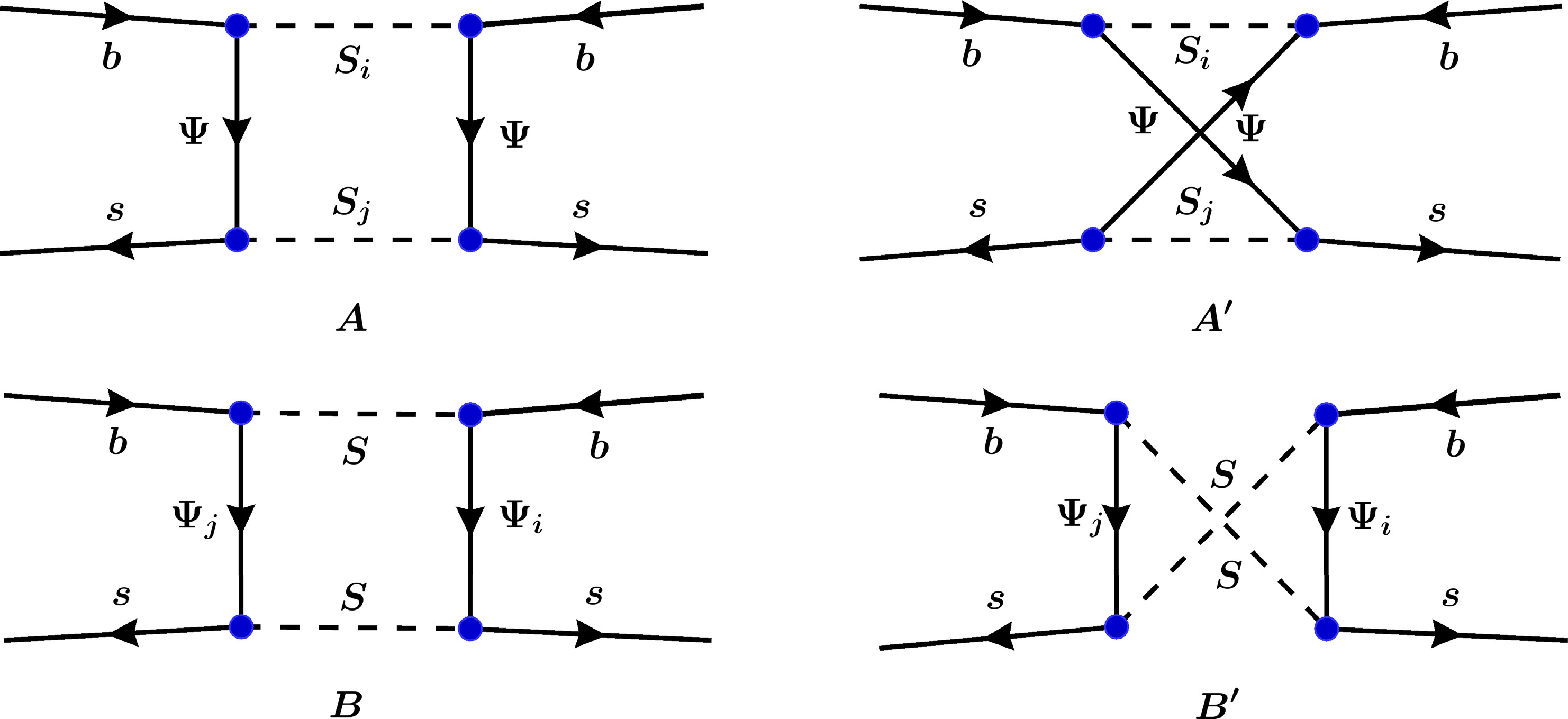

Figure 6.  (color online) One-loop diagrams contributing to $ B_s-\bar{B}_s $ mixing. The top panel shows the diagrams for the scalar-rich model, in which the standard box diagram (A) is accompanied by a "crossed-fermion" diagram (A^') if the mediator Ψ is a Majorana particle. The bottom panel shows the diagrams for the fermion-rich model, in which the standard box diagram (B) is accompanied by a "crossed-scalar" diagram (B^') if the mediator S is a real scalar. The indices $ i,j $ on the mediators denote the distinct particle species defined in each model.

In the fermion-rich model, where the scalar S can be real ($ \eta^M=1 $), we find a cancellation between the standard and crossed-box diagrams, leading to

In both sets of equations, $ \eta^M=0 $ for a complex particle (Dirac fermion or complex scalar) and $ \eta^M=1 $ otherwise.

The theoretical prediction for the $ B_s-\bar{B}_s $ mass difference, $ \Delta M_s $, is determined by the off-diagonal element of the mass matrix, with $ \Delta M_s = 2|M_{12}| $. This matrix element is calculated from the effective Hamiltonian in Eq. (32) via

where $ \langle {\cal{O}}_a\rangle(\mu) \equiv \langle B_s|{\cal{O}}_a|\bar{B}_s\rangle(\mu) $ denotes the hadronic matrix elements of the operators evaluated at the scale μ. Although both the Wilson coefficients $ C_a(\mu) $ and the matrix elements $ \langle {\cal{O}}_a\rangle(\mu) $ depend on the renormalization scale μ, the physical observable $ \Delta M_s $ is scale independent.

We compare these predictions with the precise measurement reported by the LHCb collaboration, $ \Delta M_s = (1.1693\pm 0.0004) \times 10^{-8} $ MeV [75]. For the theoretical inputs, we adopt the matrix elements calculated in the $ \overline{{\rm{MS}}} $-NDR scheme at $ \mu=4.16 $ GeV [74]:

Substituting these values into Eq. (44), we obtain the following constraint on the NP Wilson coefficients:

This inequality, together with the matching conditions in Eq. (37), directly constrains the parameter space of our benchmark models.

Another set of constraints on our models arises from their potential contributions to $ B_s-\bar{B}_s $ mixing. At low energies, this process is described by the effective Hamiltonian

Adopting the so-called BMU basis [73], the operators relevant to our analysis are listed as follows:

While the SM contribution to this process is dominated by $ {\cal{O}}_{{\rm{VLL}}} $, it is CKM-suppressed and can be safely neglected [74]. In the SMEFT framework, our benchmark models generate contributions to three of the primary $ \Delta B=2 $ operators, namely

where the subscript denotes the quark-field generation. Evaluating the SMEFT-to-LEFT matching and the RG evolution down to $ \mu = m_b $ with $\mathrm{DsixTools}$ [65, 66] yields

where an approximately 5% enhancement in $ C_{{\rm{LR}},1}(m_b) $ from RG running has been neglected.

The one-loop box diagrams that generate these SMEFT operators in our benchmark models are shown in Fig. 6. As in the previous sections, the contributions depend on whether the mediating particles are complex or real. For the scalar-rich model, in which the fermion Ψ can be a Majorana particle ($ \eta^M=1 $), we obtain

Figure 6.  (color online) One-loop diagrams contributing to $ B_s-\bar{B}_s $ mixing. The top panel shows the diagrams for the scalar-rich model, in which the standard box diagram (A) is accompanied by a "crossed-fermion" diagram (A^') if the mediator Ψ is a Majorana particle. The bottom panel shows the diagrams for the fermion-rich model, in which the standard box diagram (B) is accompanied by a "crossed-scalar" diagram (B^') if the mediator S is a real scalar. The indices $ i,j $ on the mediators denote the distinct particle species defined in each model.

In the fermion-rich model, where the scalar S can be real ($ \eta^M=1 $), we find a cancellation between the standard and crossed-box diagrams, leading to

In both sets of equations, $ \eta^M=0 $ for a complex particle (Dirac fermion or complex scalar) and $ \eta^M=1 $ otherwise.

The theoretical prediction for the $ B_s-\bar{B}_s $ mass difference, $ \Delta M_s $, is determined by the off-diagonal element of the mass matrix, with $ \Delta M_s = 2|M_{12}| $. This matrix element is calculated from the effective Hamiltonian in Eq. (32) via

where $ \langle {\cal{O}}_a\rangle(\mu) \equiv \langle B_s|{\cal{O}}_a|\bar{B}_s\rangle(\mu) $ denotes the hadronic matrix elements of the operators evaluated at the scale μ. Although both the Wilson coefficients $ C_a(\mu) $ and the matrix elements $ \langle {\cal{O}}_a\rangle(\mu) $ depend on the renormalization scale μ, the physical observable $ \Delta M_s $ is scale independent.

We compare these predictions with the precise measurement reported by the LHCb collaboration, $ \Delta M_s = (1.1693\pm 0.0004) \times 10^{-8} $ MeV [75]. For the theoretical inputs, we adopt the matrix elements calculated in the $ \overline{{\rm{MS}}} $-NDR scheme at $ \mu=4.16 $ GeV [74]:

Substituting these values into Eq. (44), we obtain the following constraint on the NP Wilson coefficients:

This inequality, together with the matching conditions in Eq. (37), directly constrains the parameter space of our benchmark models.

The radiative dipole transition $ b \to s\gamma $ also imposes stringent constraints on our models. This process is described by the effective Hamiltonian

which contains the electromagnetic and chromomagnetic dipole operators:

Here, $ F_{\mu\nu} $ and $ G_{\mu\nu}^a $ denote the electromagnetic and gluonic field-strength tensors, respectively. The process $ b \to s\gamma $ is directly governed by the Wilson coefficients $ C_7^{(\prime)} $, which also receive contributions from the QCD mixing of the coefficients $ C_8^{(\prime)} $.

In our benchmark models, these operators are generated at the one-loop level through the diagrams shown in Fig. 7. We now calculate the new-physics contributions to the Wilson coefficients, denoted by $ \Delta C_{7,8}^{(\prime)} $, for each of the two models in turn.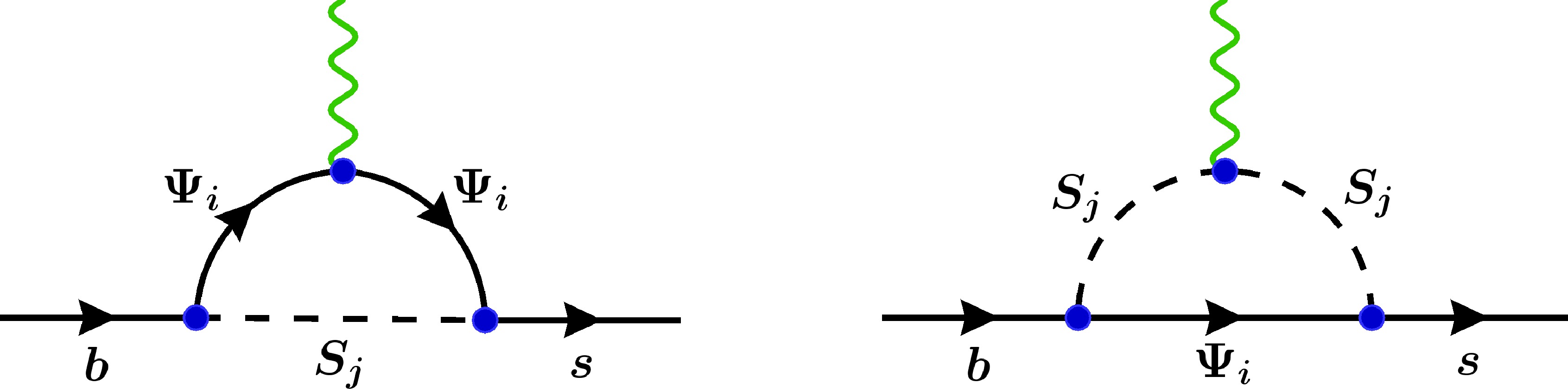

Figure 7.  (color online) One-loop contributions to $ b\rightarrow s \gamma $ in the benchmark models. Replacing the photon (wavy green line) with a gluon gives the corresponding diagrams for the chromomagnetic transition $ b\rightarrow s g $.

We first consider the scalar-rich model. In this scenario, the mediating fermion is always the color-singlet Ψ, whereas the internal scalars can be either $ S_1 $ or $ S_3 $, both of which are color anti-triplets. Integrating out these heavy particles yields the following new-physics contributions to the electromagnetic dipole coefficients:

where the mass ratios are defined as $ x_j = m_\Psi^2/m_{S_j}^2 $ for $ j=1,3 $, and the loop functions $ F_7 $ and $ \tilde{F}_7 $ are given in Appendix A. The contributions to the chromomagnetic coefficients, $ \Delta C_8^{(\prime)} $, are obtained by replacing the electric charges $ Q_X $ with the color factors $ \chi_X $. In this case, $ \chi_\Psi = 0 $ for the color-singlet Ψ, while $ \chi_{S_{1,3}} = 1 $ for the color anti-triplets $ S_{1,3} $.

Next, we analyze the fermion-rich model. Here, the mediating scalar S is a color singlet, while the internal fermions can be either $ \Psi_1 $ or $ \Psi_3 $, both of which are color triplets. The resulting NP contributions are

where the mass ratios are now defined as $ x_j = m_{\Psi_j}^2/m_{S}^2 $. The corresponding chromomagnetic coefficients $ \Delta C_8^{(\prime)} $ are again obtained by replacing the electric charges with color factors. Specifically, $ \chi_S=0 $ for the color scalar S, and $ \chi_{\Psi_{1,3}}=1 $ for the color triplets $ \Psi_{1,3} $.

The theoretical prediction for the branching ratio, including the photon-energy cut $ E_\gamma \gt E_0 = 1.6\,{\rm{GeV}} $, can be separated into the SM prediction and the NP correction:

The NP contribution, $ \delta\overline{{\cal{B}}}(b \to s\gamma) $, evaluated at the scale $ \mu = 160\;{\rm{GeV}} $, is given by [76, 77]

For our analysis, we have considered only the leading-order contributions to $ \Delta{\cal{C}}_{7,8}^{(\prime)} $. For the complete next-to-leading-order expression, we refer the reader to the original references.

The current world average of the experimental branching ratio is [62]:

Compared with the SM prediction at NNLO [78]:

The difference between the experimental value and the SM prediction provides a window into new physics. By requiring our calculated NP contribution, $ \delta\overline{{\cal{B}}}(b \to s\gamma) $, to be consistent with this window, we can place a direct constraint on the NP Wilson coefficients $ \Delta C_{7,8}^{(\prime)} $.

The radiative dipole transition $ b \to s\gamma $ also imposes stringent constraints on our models. This process is described by the effective Hamiltonian

which contains the electromagnetic and chromomagnetic dipole operators:

Here, $ F_{\mu\nu} $ and $ G_{\mu\nu}^a $ denote the electromagnetic and gluonic field-strength tensors, respectively. The process $ b \to s\gamma $ is directly governed by the Wilson coefficients $ C_7^{(\prime)} $, which also receive contributions from the QCD mixing of the coefficients $ C_8^{(\prime)} $.

In our benchmark models, these operators are generated at the one-loop level through the diagrams shown in Fig. 7. We now calculate the new-physics contributions to the Wilson coefficients, denoted by $ \Delta C_{7,8}^{(\prime)} $, for each of the two models in turn.

Figure 7.  (color online) One-loop contributions to $ b\rightarrow s \gamma $ in the benchmark models. Replacing the photon (wavy green line) with a gluon gives the corresponding diagrams for the chromomagnetic transition $ b\rightarrow s g $.

We first consider the scalar-rich model. In this scenario, the mediating fermion is always the color-singlet Ψ, whereas the internal scalars can be either $ S_1 $ or $ S_3 $, both of which are color anti-triplets. Integrating out these heavy particles yields the following new-physics contributions to the electromagnetic dipole coefficients:

where the mass ratios are defined as $ x_j = m_\Psi^2/m_{S_j}^2 $ for $ j=1,3 $, and the loop functions $ F_7 $ and $ \tilde{F}_7 $ are given in Appendix A. The contributions to the chromomagnetic coefficients, $ \Delta C_8^{(\prime)} $, are obtained by replacing the electric charges $ Q_X $ with the color factors $ \chi_X $. In this case, $ \chi_\Psi = 0 $ for the color-singlet Ψ, while $ \chi_{S_{1,3}} = 1 $ for the color anti-triplets $ S_{1,3} $.

Next, we analyze the fermion-rich model. Here, the mediating scalar S is a color singlet, while the internal fermions can be either $ \Psi_1 $ or $ \Psi_3 $, both of which are color triplets. The resulting NP contributions are

where the mass ratios are now defined as $ x_j = m_{\Psi_j}^2/m_{S}^2 $. The corresponding chromomagnetic coefficients $ \Delta C_8^{(\prime)} $ are again obtained by replacing the electric charges with color factors. Specifically, $ \chi_S=0 $ for the color scalar S, and $ \chi_{\Psi_{1,3}}=1 $ for the color triplets $ \Psi_{1,3} $.

The theoretical prediction for the branching ratio, including the photon-energy cut $ E_\gamma \gt E_0 = 1.6\,{\rm{GeV}} $, can be separated into the SM prediction and the NP correction:

The NP contribution, $ \delta\overline{{\cal{B}}}(b \to s\gamma) $, evaluated at the scale $ \mu = 160\;{\rm{GeV}} $, is given by [76, 77]

For our analysis, we have considered only the leading-order contributions to $ \Delta{\cal{C}}_{7,8}^{(\prime)} $. For the complete next-to-leading-order expression, we refer the reader to the original references.

The current world average of the experimental branching ratio is [62]:

Compared with the SM prediction at NNLO [78]:

The difference between the experimental value and the SM prediction provides a window into new physics. By requiring our calculated NP contribution, $ \delta\overline{{\cal{B}}}(b \to s\gamma) $, to be consistent with this window, we can place a direct constraint on the NP Wilson coefficients $ \Delta C_{7,8}^{(\prime)} $.

Additional constraints arise from radiative corrections to the effective Z-boson couplings to SM fermions. We consider contributions that affect both on-shell Z decay vertices and off-shell Z-exchange amplitudes. Using the detailed analytical expressions for the generic one-loop functions provided in Appendix B, we focus here on their application to the specific interaction structures of our two benchmark models.

For the scalar-rich model, the fermion sector contains a single SU(2)_L-singlet vector-like fermion Ψ. Using the notation of Eq. (B4), its couplings to the Z boson are given by:

Regarding the scalar fields, we organize them into multiplets $ \Phi_M $ to match the generic formalism. We explicitly label their components by their electric charges (denoted by superscripts) and group them as follows:

The components of $ \Phi_1 $ couple to down-type quarks $ d_i $, whereas those of $ \Phi_2 $ couple to left-handed neutrinos $ \nu_i $. In addition, $ \Phi_4 $ couples to charged leptons $ e_i $, while $ \Phi_3 $ interacts with the corresponding charge-conjugated fields $ e^{c}_{i} $. We omit the component $ S^{\alpha-2/3}_3 $, as it couples exclusively to up-type quarks. The corresponding Z-coupling matrices $ g^{\Phi_M} $ (cf. Eq. (B4)) are given by

where the relevant electric charges are $ Q_{\Phi_1}=\alpha+1/3 $, $ Q_{\Phi_2}=\alpha $, $ Q_{\Phi_3}=\alpha-1 $, and $ Q_{\Phi_4}=\alpha+1 $.

Turning to the fermion-rich model, the scalar sector consists of a single SU(2)_L singlet field S, whose coupling to the Z boson is determined solely by its charge:

The vector-like fermion sector contains multiple fields. Labeling the fermion components by their electric charges, we define the multiplets $ F_{1,2,3} $ as follows:

The component $ \Psi^{\alpha+1}_3 $ is not shown because it couples exclusively to up-type quarks. The corresponding Z couplings of the multiplets $ F_{1,2,3} $ (cf. Eq. (B4)) are given by

where the relevant electric charges are $ Q_{F_1}=\alpha $, $ Q_{F_2}= \alpha+1/3 $, and $ Q_{F_3}=\alpha-2/3 $.

With the couplings and field components established, we next calculate the one-loop corrections to the decay modes $ Z\to \bar{s}b $, $ \tau^+\tau^- $, and $ \nu_{\tau}\bar{\nu}_{\tau} $. In the scalar-rich model, the contributions to the effective couplings are given by:

for the quark modes. For the leptonic modes, we must account for the color charge of the internal NP fields, which yields an enhancement factor of $ \chi_Z = 3 $. The resulting expressions are:

Here, $ M_{S_i} $ ($ i=1,\cdots,4 $) and $ M_{\Psi} $ denote the masses of the scalar fields $ S_{i} $ and the fermion Ψ, respectively. We define the mass ratios as $ x_i \equiv M^2_{\Psi}/M^2_{S_i} $.

Similarly, within the fermion-rich model, we calculate the one-loop corrections to the $ Z \to \bar{s}b $, $ \tau^+\tau^- $, and $ \nu_\tau \bar{\nu}_\tau $ decay channels. The resulting contributions to the effective form factors are given by

for the quark sector, and

for the lepton sector. Here, $ M_{S} $ and $ M_{\Psi_k} $ (with $ k=1,2,3 $) denote the masses of the scalar field S and the vector-like fermions $ \Psi_k $, respectively. The mass ratios are defined by $ y_k = M^2_{\Psi_k}/M^2_{S} $.

To constrain the new-physics parameters, we use the precision measurements of Z-pole observables performed at LEP [79]. Following the analysis in Refs. [80, 81], we adopt the following model-independent bounds on the effective leptonic form factors ²:

Regarding the $ Z \to \bar{s}b $ decay, we apply the upper limit $ {\cal{B}}(Z\to q\bar{q}^\prime) \lt 2.9 \times 10^{-3} $ at 95% C.L., derived from the agreement between the measured hadronic Z width and the SM prediction [82, 83]. Since the SM contribution to this mode is negligible relative to the current experimental sensitivity [83], we assume that the decay is dominated by the NP contribution. This leads to the constraint:

where $ \Gamma_Z $ is the total decay width of the Z boson. These constraints are subsequently used to delineate the viable parameter space of the couplings in both benchmark models.

Additional constraints arise from radiative corrections to the effective Z-boson couplings to SM fermions. We consider contributions that affect both on-shell Z decay vertices and off-shell Z-exchange amplitudes. Using the detailed analytical expressions for the generic one-loop functions provided in Appendix B, we focus here on their application to the specific interaction structures of our two benchmark models.

For the scalar-rich model, the fermion sector contains a single SU(2)_L-singlet vector-like fermion Ψ. Using the notation of Eq. (B4), its couplings to the Z boson are given by:

Regarding the scalar fields, we organize them into multiplets $ \Phi_M $ to match the generic formalism. We explicitly label their components by their electric charges (denoted by superscripts) and group them as follows:

The components of $ \Phi_1 $ couple to down-type quarks $ d_i $, whereas those of $ \Phi_2 $ couple to left-handed neutrinos $ \nu_i $. In addition, $ \Phi_4 $ couples to charged leptons $ e_i $, while $ \Phi_3 $ interacts with the corresponding charge-conjugated fields $ e^{c}_{i} $. We omit the component $ S^{\alpha-2/3}_3 $, as it couples exclusively to up-type quarks. The corresponding Z-coupling matrices $ g^{\Phi_M} $ (cf. Eq. (B4)) are given by

where the relevant electric charges are $ Q_{\Phi_1}=\alpha+1/3 $, $ Q_{\Phi_2}=\alpha $, $ Q_{\Phi_3}=\alpha-1 $, and $ Q_{\Phi_4}=\alpha+1 $.

Turning to the fermion-rich model, the scalar sector consists of a single SU(2)_L singlet field S, whose coupling to the Z boson is determined solely by its charge:

The vector-like fermion sector contains multiple fields. Labeling the fermion components by their electric charges, we define the multiplets $ F_{1,2,3} $ as follows:

The component $ \Psi^{\alpha+1}_3 $ is not shown because it couples exclusively to up-type quarks. The corresponding Z couplings of the multiplets $ F_{1,2,3} $ (cf. Eq. (B4)) are given by

where the relevant electric charges are $ Q_{F_1}=\alpha $, $ Q_{F_2}= \alpha+1/3 $, and $ Q_{F_3}=\alpha-2/3 $.

With the couplings and field components established, we next calculate the one-loop corrections to the decay modes $ Z\to \bar{s}b $, $ \tau^+\tau^- $, and $ \nu_{\tau}\bar{\nu}_{\tau} $. In the scalar-rich model, the contributions to the effective couplings are given by:

for the quark modes. For the leptonic modes, we must account for the color charge of the internal NP fields, which yields an enhancement factor of $ \chi_Z = 3 $. The resulting expressions are:

Here, $ M_{S_i} $ ($ i=1,\cdots,4 $) and $ M_{\Psi} $ denote the masses of the scalar fields $ S_{i} $ and the fermion Ψ, respectively. We define the mass ratios as $ x_i \equiv M^2_{\Psi}/M^2_{S_i} $.

Similarly, within the fermion-rich model, we calculate the one-loop corrections to the $ Z \to \bar{s}b $, $ \tau^+\tau^- $, and $ \nu_\tau \bar{\nu}_\tau $ decay channels. The resulting contributions to the effective form factors are given by

for the quark sector, and

for the lepton sector. Here, $ M_{S} $ and $ M_{\Psi_k} $ (with $ k=1,2,3 $) denote the masses of the scalar field S and the vector-like fermions $ \Psi_k $, respectively. The mass ratios are defined by $ y_k = M^2_{\Psi_k}/M^2_{S} $.

To constrain the new-physics parameters, we use the precision measurements of Z-pole observables performed at LEP [79]. Following the analysis in Refs. [80, 81], we adopt the following model-independent bounds on the effective leptonic form factors ²:

Regarding the $ Z \to \bar{s}b $ decay, we apply the upper limit $ {\cal{B}}(Z\to q\bar{q}^\prime) \lt 2.9 \times 10^{-3} $ at 95% C.L., derived from the agreement between the measured hadronic Z width and the SM prediction [82, 83]. Since the SM contribution to this mode is negligible relative to the current experimental sensitivity [83], we assume that the decay is dominated by the NP contribution. This leads to the constraint:

where $ \Gamma_Z $ is the total decay width of the Z boson. These constraints are subsequently used to delineate the viable parameter space of the couplings in both benchmark models.

Having established the analytical bounds from individual decay channels, we now perform a combined analysis to delineate the viable parameter space. We begin by defining benchmark masses for the new particles that are consistent with direct LHC searches. We then map the allowed regions for the Yukawa couplings under specific degeneracy schemes. Finally, we evaluate the maximum attainable branching ratios for $ B \to K^{(*)} \nu \bar{\nu} $ permitted by the global data.

We first establish benchmark values for the masses of the new scalars and fermions. For the fermion-rich model, following the analysis in Ref. [81] and to ensure consistency with current bounds [84, 85], we set the masses of the colored fermions to $ M_{\Psi_1}=M_{\Psi_3}=3.15 $ TeV, while assigning a moderate mass of $ 450 $ GeV to the scalar S and the fermion $ \Psi_2 $ ($ M_{S}=M_{\Psi_2}=450 $ GeV). This mass spectrum places the model well beyond the reach of direct LHC searches [86].

For the scalar-rich model, we choose the mass spectrum of the color-singlet sector to match that of the previous case, setting $ M_{\Psi}=M_{S_2}=M_{S_4}=450 $ GeV. This choice is justified because these fields are colorless and have quantum numbers similar to those of their counterparts in the fermion-rich model (S and $ \Psi_2 $), implying comparable phenomenological constraints. The masses of the colored scalars $ S_{1,3} $ are then constrained by their decays into the fermion Ψ. Analyses of $ 36\; {\rm{fb}}^{-1} $ of data at $ \sqrt{s} = 13 $ TeV [87, 88] indicate that, for $ M_{\Psi}=450 $ GeV, the lower bound on the colored scalar mass is approximately $ 1.10 $ TeV.

Accordingly, we define the following two benchmark points (BPs):

● BP-I (Scalar-rich): $ M_{\Psi}=M_{S_2}=M_{S_4}=450 $ GeV, and $ M_{S_1}=M_{S_3}=1.10 $ TeV.

● BP-II (fermion-rich): $ M_{S}=M_{\Psi_2}=450 $ GeV, $ M_{\Psi_1}= M_{\Psi_3}=3.15 $ TeV.

With the mass spectra established, we proceed to constrain the coupling constants. We require all dimensionless couplings to satisfy the perturbative unitarity condition, $ |g| \le 1 $, and, for simplicity, assume them to be real. While the fermion-rich model is characterized by five couplings, $ \{g^3_1, g^2_1, g^3_{1'}, g^2_{1'}, g_2^3\} $, the scalar-rich model nominally introduces a sixth, $ \{g^3_1, g^2_1, g^3_{1'}, g^2_{1'}, g_2^3, g_{2'}^3\} $. To simplify the analysis, we reduce the parameter space of the scalar-rich model by assuming $ g_2^3 = g_{2'}^3 $, resulting in five independent constants in both models.

We note that the constraints derived from $ B_s-\bar{B}_s $ mixing, $ b \to s\gamma $, and $ Z \to b\bar{s} $ act exclusively on the quark-sector couplings ($ g^3_1, g^2_1, g^3_{1'}, g^2_{1'} $). Similarly, the leptonic Z-pole observables ($ Z\to \tau^+\tau^- $ and $ Z\to \nu_{\tau} \bar{\nu}_{\tau} $) depend solely on the lepton coupling $ g_2^3 $ (and $ g_{2'}^3 $). We therefore use these processes to constrain the quark and lepton couplings independently. Our numerical analysis shows that the quark-sector couplings are tightly constrained by $ B_s- \bar{B}_s $ mixing and $ b \to s\gamma $. By contrast, for the lepton coupling, the bounds from the leptonic Z-pole observables are weaker than the perturbative unitarity requirement.

In contrast, the semileptonic decays ($ B \to K^{(*)} \nu \bar{\nu} $ and $ b \to s \tau^+\tau^- $) depend on the full set of couplings, making a direct analytical inversion of the experimental limits infeasible. We therefore treat the bounds from these processes as additional conditions when determining the global maxima of the branching ratios $ {\cal{B}}(B^+ \to K^+ \nu \bar{\nu}) $ and $ {\cal{B}}(B^0 \to K^{*0} \nu \bar{\nu}) $ within the parameter space allowed by the quark- and lepton-sector constraints.

To further simplify the phenomenological analysis of the remaining five free parameters ($ g^3_1, g^2_1, g^3_{1'}, g^2_{1'}, g_2^3 $), we consider four distinct flavor structures for the quark couplings. In determining the allowed parameter space shown in Fig. 8, we conservatively incorporate theoretical uncertainties by adopting their upper error bounds, thereby imposing more stringent limits on the couplings. We have verified that varying these uncertainties within their standard ranges does not significantly affect the resulting exclusion boundaries or our qualitative conclusions. The four flavor structures are defined as follows: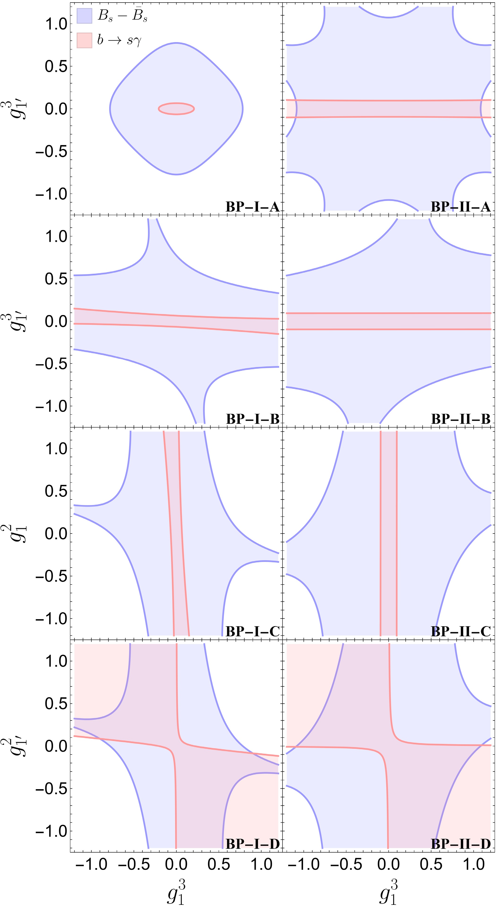

Figure 8.  (color online) Allowed regions of the quark couplings in the scalar-rich (BP-I) and fermion-rich (BP-II) models for flavor structures A–D. The blue and red shaded regions represent the parameter space consistent with the constraints from $ B_s-\bar{B}_s $ mixing and $ b \to s\gamma $, respectively. The boundaries are derived from experimental limits, with theoretical uncertainties conservatively incorporated by adopting the upper error bounds, thereby imposing more stringent constraints on the couplings. The corresponding benchmark model and flavor scheme are indicated in the bottom-right corner of each panel.

● Structure A: $ g^3_1=g^2_1, \, g^3_{1'}=g^2_{1'} $.

As illustrated in the BP-I-A panel of Fig. 8, the constraint from $ b \to s\gamma $ is generally more stringent than that from $ B_s-\bar{B}_s $ mixing. Under this structure, the scalar-rich model (BP-I) is subject to significantly stronger constraints than the fermion-rich model (BP-II). Specifically, the viable parameter space for BP-I-A is confined to a small, closed region, restricting $ g^3_{1} $ to the interval $ [-0.21, 0.21] $ and $ g^3_{1'} $ to $ [-0.07, 0.07] $. In contrast, in BP-II-A, the $ b \to s\gamma $ constraint appears as a horizontal band extending across the entire perturbative range of $ g^3_{1} $. Consequently, while $ g^3_{1} $ remains effectively unconstrained, $ g^3_{1'} $ is limited to a narrow interval, reaching its minimum width of $ [-0.10, 0.10] $ at $ g^3_{1}=0 $.

● Structure B: $ g^2_1=g^3_{1'}=g^2_{1'} $.

As shown in the panels labeled BP-I-B and BP-II-B in Fig. 8, $ g^3_1 $ remains largely unconstrained within the perturbative range $ [-1,1] $ in both models, whereas the common coupling is tightly constrained by $ b \to s\gamma $. Specifically, the common coupling is limited to approximately $ \pm 0.07 $ for BP-I and $ \pm 0.10 $ for BP-II.

● Structure C: $ g^3_1=g^3_{1'}=g^2_{1'} $.

The resulting allowed regions, shown in panels BP-I-C and BP-II-C of Fig. 8, are effectively the mirror images of those for structure B, with the axes interchanged. This reflects the symmetric role these couplings play in the loop functions. Accordingly, the stringent constraints now apply to the group of couplings fixed to $ g^3_1 $, while $ g^2_1 $ remains unconstrained over the range $ [-1,1] $ in both models.

● Structure D: $ g^3_1=g^2_1=g^3_{1'} $.

As shown in the BP-I-D and BP-II-D panels of Fig. 8, the viable parameter space is notably larger than in the previous schemes, indicating that decoupling $ g^2_{1'} $ from the other parameters provides substantial freedom to satisfy the flavor structures. We observe that the allowed regions generally favor scenarios in which $ g^3_1 $ and $ g^2_{1'} $ have opposite signs.

With the allowed parameter space established, we now determine the upper bounds on the branching ratios $ {\cal{B}}(B^+\to K^+\nu\bar{\nu}) $ and $ {\cal{B}}(B^0\to K^{*0}\nu\bar{\nu}) $, as well as the predicted ratio R. Independent numerical optimizations are performed for each benchmark model across structures A–D, with the objective of maximizing either the charged or the neutral decay channel. The resulting optimal values, together with the form-factor uncertainties, are compiled in Table 4. For each case, we report the global maximum $ {\cal{B}}_{{\rm{max}}} $, the parameter configuration $ [x, y, z] $ at which it occurs, the predicted branching fraction for the complementary channel, and the corresponding value of R.

In the case of BP-I-A, we find that NP contributions tend to suppress the neutral mode $ B^0 \to K^{*0}\nu\bar{\nu} $. Consequently, its maximum branching ratio coincides with the SM limit ³, represented by parameter configurations such as $ (x, 0, 0) $, where the vanishing quark couplings ($ y=z=0 $) render the lepton coupling x irrelevant. The opposite scenario is $ (0, y, z) $, where the lepton coupling vanishes and all effects arise solely from the quark couplings. Conversely, maximizing the $ B^+\to K^+\nu\bar{\nu} $ rate yields a modest 0.21% enhancement in the central value relative to the SM prediction; at this point, the predicted rate for the neutral mode falls slightly below its SM value. This anti-correlation indicates that a simultaneous maximization of both decay modes is not possible under flavor structure A. A similar anti-correlation is observed for BP-I-B and BP-I-C, although a small 0.60% enhancement in the central value can be achieved for the neutral mode.

Flavor structure D (BP-I-D), however, exhibits a distinct phenomenology: NP contributions can interfere constructively in both channels, allowing maximal central-value enhancements of 9.85% and 2.62% for the charged and neutral modes, respectively. Notably, at the parameter point where the neutral mode is maximized, the charged mode is also enhanced by 6.08% relative to the SM, leading to a 3.83% reduction in the central value of R. However, when the charged mode is further maximized up to $ 5.24\times10^{-6} $, the predicted rate for the neutral mode decreases to $ 9.71\times10^{-6} $, again indicating an anti-correlated behavior between the two decay channels.

Turning to the fermion-rich model (BP-II), structure A exhibits the opposite behavior to the scalar-rich model: NP contributions tend to suppress the charged mode $ B^+\to K^+\nu\bar{\nu} $, limiting its maximum to the SM value of $ 4.77\times 10^{-6} $ through configurations such as $ (x, 0, 0) $ or $ (0, y, z) $. When the neutral mode $ B^0 \to K^{*0}\nu\bar{\nu} $ is maximized to $ 1.01\times 10^{-5} $ (a 1.61% enhancement), the charged mode decreases to $ 4.64\times 10^{-6} $, thereby increasing the ratio R to 2.18. Structures B and C in BP-II follow the same anti-correlation observed in BP-I, where any enhancement in one mode forces the complementary mode below its SM expectation.

In contrast, structure D (BP-II-D) allows constructive interference in both channels simultaneously. Specifically, at the parameter point that maximizes the neutral mode ($ {\cal{B}}_{{\rm{max}}} = 1.02\times 10^{-5} $, a 2.62% enhancement), the charged mode simultaneously reaches $ 4.80\times 10^{-6} $ (a $ 0.63\% $ enhancement), which matches the maximum value obtained in the dedicated charged-mode scan. In the reverse optimization, the neutral-mode rate at the charged maximum reaches $ 1.01\times 10^{-5} $. Because the relative enhancement in the neutral channel exceeds that in the charged channel, the central value of R increases from 2.09 to 2.12.

As listed in Table 4, the absolute branching fractions across all flavor structures (A–D) and both benchmark models are subject to hadronic form-factor uncertainties. These uncertainties are nearly uniform across all entries, amounting to roughly $ \pm $ 4% for $ {\cal{B}}(B^+\to K^+\nu\bar{\nu}) $, $ \pm $ 20% for $ {\cal{B}}(B^0\to K^{*0}\nu\bar{\nu}) $, and $ \pm $ 25% for the ratio R, largely dominated by the hadronic matrix elements in the $ B\to K^* $ transition. Taking these theoretical uncertainties into account, the lowest attainable ratio across all investigated scenarios is $ R \approx 1.41 $, realized in $ \text{BP-I-D} $ under the $ B^+\to K^+\nu\bar{\nu} $ optimization.

We conclude this section by considering the simplest flavor structure, namely $ g^3_1 = g^2_1 = g^3_{1'} = g^2_{1'} $. As is evident from Eqs. (10) and (11), the scalar-rich model under the BP-I mass scheme yields $ [C_{\ell q}^{(1)}]_{\ell\ell23} = -[C_{\ell d}]_{\ell\ell23} $, or equivalently, $ \Delta C_L^{\nu_\ell} = -\Delta C_R^{\nu_\ell} $. Because the $ B^+\to K^+\nu\bar{\nu} $ amplitude depends on the combination $ (\Delta C_L^{\nu_\ell} + \Delta C_R^{\nu_\ell}) $, this exact cancellation implies that NP contributions to the charged mode vanish identically, leaving its branching fraction at the SM prediction. Conversely, for the fermion-rich model under the BP-II mass scheme, this same flavor structure results in $ \Delta C_L^{\nu_\ell} = \Delta C_R^{\nu_\ell} $. Nevertheless, because the relevant loop function $ J_4 $ is negative, the resulting NP loop effects interfere destructively, suppressing both decay modes below their SM expectations.

Having established the analytical bounds from individual decay channels, we now perform a combined analysis to delineate the viable parameter space. We begin by defining benchmark masses for the new particles that are consistent with direct LHC searches. We then map the allowed regions for the Yukawa couplings under specific degeneracy schemes. Finally, we evaluate the maximum attainable branching ratios for $ B \to K^{(*)} \nu \bar{\nu} $ permitted by the global data.

We first establish benchmark values for the masses of the new scalars and fermions. For the fermion-rich model, following the analysis in Ref. [81] and to ensure consistency with current bounds [84, 85], we set the masses of the colored fermions to $ M_{\Psi_1}=M_{\Psi_3}=3.15 $ TeV, while assigning a moderate mass of $ 450 $ GeV to the scalar S and the fermion $ \Psi_2 $ ($ M_{S}=M_{\Psi_2}=450 $ GeV). This mass spectrum places the model well beyond the reach of direct LHC searches [86].

For the scalar-rich model, we choose the mass spectrum of the color-singlet sector to match that of the previous case, setting $ M_{\Psi}=M_{S_2}=M_{S_4}=450 $ GeV. This choice is justified because these fields are colorless and have quantum numbers similar to those of their counterparts in the fermion-rich model (S and $ \Psi_2 $), implying comparable phenomenological constraints. The masses of the colored scalars $ S_{1,3} $ are then constrained by their decays into the fermion Ψ. Analyses of $ 36\; {\rm{fb}}^{-1} $ of data at $ \sqrt{s} = 13 $ TeV [87, 88] indicate that, for $ M_{\Psi}=450 $ GeV, the lower bound on the colored scalar mass is approximately $ 1.10 $ TeV.

Accordingly, we define the following two benchmark points (BPs):

● BP-I (Scalar-rich): $ M_{\Psi}=M_{S_2}=M_{S_4}=450 $ GeV, and $ M_{S_1}=M_{S_3}=1.10 $ TeV.

● BP-II (fermion-rich): $ M_{S}=M_{\Psi_2}=450 $ GeV, $ M_{\Psi_1}= M_{\Psi_3}=3.15 $ TeV.

With the mass spectra established, we proceed to constrain the coupling constants. We require all dimensionless couplings to satisfy the perturbative unitarity condition, $ |g| \le 1 $, and, for simplicity, assume them to be real. While the fermion-rich model is characterized by five couplings, $ \{g^3_1, g^2_1, g^3_{1'}, g^2_{1'}, g_2^3\} $, the scalar-rich model nominally introduces a sixth, $ \{g^3_1, g^2_1, g^3_{1'}, g^2_{1'}, g_2^3, g_{2'}^3\} $. To simplify the analysis, we reduce the parameter space of the scalar-rich model by assuming $ g_2^3 = g_{2'}^3 $, resulting in five independent constants in both models.

We note that the constraints derived from $ B_s-\bar{B}_s $ mixing, $ b \to s\gamma $, and $ Z \to b\bar{s} $ act exclusively on the quark-sector couplings ($ g^3_1, g^2_1, g^3_{1'}, g^2_{1'} $). Similarly, the leptonic Z-pole observables ($ Z\to \tau^+\tau^- $ and $ Z\to \nu_{\tau} \bar{\nu}_{\tau} $) depend solely on the lepton coupling $ g_2^3 $ (and $ g_{2'}^3 $). We therefore use these processes to constrain the quark and lepton couplings independently. Our numerical analysis shows that the quark-sector couplings are tightly constrained by $ B_s- \bar{B}_s $ mixing and $ b \to s\gamma $. By contrast, for the lepton coupling, the bounds from the leptonic Z-pole observables are weaker than the perturbative unitarity requirement.

In contrast, the semileptonic decays ($ B \to K^{(*)} \nu \bar{\nu} $ and $ b \to s \tau^+\tau^- $) depend on the full set of couplings, making a direct analytical inversion of the experimental limits infeasible. We therefore treat the bounds from these processes as additional conditions when determining the global maxima of the branching ratios $ {\cal{B}}(B^+ \to K^+ \nu \bar{\nu}) $ and $ {\cal{B}}(B^0 \to K^{*0} \nu \bar{\nu}) $ within the parameter space allowed by the quark- and lepton-sector constraints.

To further simplify the phenomenological analysis of the remaining five free parameters ($ g^3_1, g^2_1, g^3_{1'}, g^2_{1'}, g_2^3 $), we consider four distinct flavor structures for the quark couplings. In determining the allowed parameter space shown in Fig. 8, we conservatively incorporate theoretical uncertainties by adopting their upper error bounds, thereby imposing more stringent limits on the couplings. We have verified that varying these uncertainties within their standard ranges does not significantly affect the resulting exclusion boundaries or our qualitative conclusions. The four flavor structures are defined as follows:

Figure 8.  (color online) Allowed regions of the quark couplings in the scalar-rich (BP-I) and fermion-rich (BP-II) models for flavor structures A–D. The blue and red shaded regions represent the parameter space consistent with the constraints from $ B_s-\bar{B}_s $ mixing and $ b \to s\gamma $, respectively. The boundaries are derived from experimental limits, with theoretical uncertainties conservatively incorporated by adopting the upper error bounds, thereby imposing more stringent constraints on the couplings. The corresponding benchmark model and flavor scheme are indicated in the bottom-right corner of each panel.

● Structure A: $ g^3_1=g^2_1, \, g^3_{1'}=g^2_{1'} $.

As illustrated in the BP-I-A panel of Fig. 8, the constraint from $ b \to s\gamma $ is generally more stringent than that from $ B_s-\bar{B}_s $ mixing. Under this structure, the scalar-rich model (BP-I) is subject to significantly stronger constraints than the fermion-rich model (BP-II). Specifically, the viable parameter space for BP-I-A is confined to a small, closed region, restricting $ g^3_{1} $ to the interval $ [-0.21, 0.21] $ and $ g^3_{1'} $ to $ [-0.07, 0.07] $. In contrast, in BP-II-A, the $ b \to s\gamma $ constraint appears as a horizontal band extending across the entire perturbative range of $ g^3_{1} $. Consequently, while $ g^3_{1} $ remains effectively unconstrained, $ g^3_{1'} $ is limited to a narrow interval, reaching its minimum width of $ [-0.10, 0.10] $ at $ g^3_{1}=0 $.

● Structure B: $ g^2_1=g^3_{1'}=g^2_{1'} $.

As shown in the panels labeled BP-I-B and BP-II-B in Fig. 8, $ g^3_1 $ remains largely unconstrained within the perturbative range $ [-1,1] $ in both models, whereas the common coupling is tightly constrained by $ b \to s\gamma $. Specifically, the common coupling is limited to approximately $ \pm 0.07 $ for BP-I and $ \pm 0.10 $ for BP-II.

● Structure C: $ g^3_1=g^3_{1'}=g^2_{1'} $.

The resulting allowed regions, shown in panels BP-I-C and BP-II-C of Fig. 8, are effectively the mirror images of those for structure B, with the axes interchanged. This reflects the symmetric role these couplings play in the loop functions. Accordingly, the stringent constraints now apply to the group of couplings fixed to $ g^3_1 $, while $ g^2_1 $ remains unconstrained over the range $ [-1,1] $ in both models.

● Structure D: $ g^3_1=g^2_1=g^3_{1'} $.

As shown in the BP-I-D and BP-II-D panels of Fig. 8, the viable parameter space is notably larger than in the previous schemes, indicating that decoupling $ g^2_{1'} $ from the other parameters provides substantial freedom to satisfy the flavor structures. We observe that the allowed regions generally favor scenarios in which $ g^3_1 $ and $ g^2_{1'} $ have opposite signs.

With the allowed parameter space established, we now determine the upper bounds on the branching ratios $ {\cal{B}}(B^+\to K^+\nu\bar{\nu}) $ and $ {\cal{B}}(B^0\to K^{*0}\nu\bar{\nu}) $, as well as the predicted ratio R. Independent numerical optimizations are performed for each benchmark model across structures A–D, with the objective of maximizing either the charged or the neutral decay channel. The resulting optimal values, together with the form-factor uncertainties, are compiled in Table 4. For each case, we report the global maximum $ {\cal{B}}_{{\rm{max}}} $, the parameter configuration $ [x, y, z] $ at which it occurs, the predicted branching fraction for the complementary channel, and the corresponding value of R.

In the case of BP-I-A, we find that NP contributions tend to suppress the neutral mode $ B^0 \to K^{*0}\nu\bar{\nu} $. Consequently, its maximum branching ratio coincides with the SM limit ³, represented by parameter configurations such as $ (x, 0, 0) $, where the vanishing quark couplings ($ y=z=0 $) render the lepton coupling x irrelevant. The opposite scenario is $ (0, y, z) $, where the lepton coupling vanishes and all effects arise solely from the quark couplings. Conversely, maximizing the $ B^+\to K^+\nu\bar{\nu} $ rate yields a modest 0.21% enhancement in the central value relative to the SM prediction; at this point, the predicted rate for the neutral mode falls slightly below its SM value. This anti-correlation indicates that a simultaneous maximization of both decay modes is not possible under flavor structure A. A similar anti-correlation is observed for BP-I-B and BP-I-C, although a small 0.60% enhancement in the central value can be achieved for the neutral mode.

Flavor structure D (BP-I-D), however, exhibits a distinct phenomenology: NP contributions can interfere constructively in both channels, allowing maximal central-value enhancements of 9.85% and 2.62% for the charged and neutral modes, respectively. Notably, at the parameter point where the neutral mode is maximized, the charged mode is also enhanced by 6.08% relative to the SM, leading to a 3.83% reduction in the central value of R. However, when the charged mode is further maximized up to $ 5.24\times10^{-6} $, the predicted rate for the neutral mode decreases to $ 9.71\times10^{-6} $, again indicating an anti-correlated behavior between the two decay channels.

Turning to the fermion-rich model (BP-II), structure A exhibits the opposite behavior to the scalar-rich model: NP contributions tend to suppress the charged mode $ B^+\to K^+\nu\bar{\nu} $, limiting its maximum to the SM value of $ 4.77\times 10^{-6} $ through configurations such as $ (x, 0, 0) $ or $ (0, y, z) $. When the neutral mode $ B^0 \to K^{*0}\nu\bar{\nu} $ is maximized to $ 1.01\times 10^{-5} $ (a 1.61% enhancement), the charged mode decreases to $ 4.64\times 10^{-6} $, thereby increasing the ratio R to 2.18. Structures B and C in BP-II follow the same anti-correlation observed in BP-I, where any enhancement in one mode forces the complementary mode below its SM expectation.

In contrast, structure D (BP-II-D) allows constructive interference in both channels simultaneously. Specifically, at the parameter point that maximizes the neutral mode ($ {\cal{B}}_{{\rm{max}}} = 1.02\times 10^{-5} $, a 2.62% enhancement), the charged mode simultaneously reaches $ 4.80\times 10^{-6} $ (a $ 0.63\% $ enhancement), which matches the maximum value obtained in the dedicated charged-mode scan. In the reverse optimization, the neutral-mode rate at the charged maximum reaches $ 1.01\times 10^{-5} $. Because the relative enhancement in the neutral channel exceeds that in the charged channel, the central value of R increases from 2.09 to 2.12.

As listed in Table 4, the absolute branching fractions across all flavor structures (A–D) and both benchmark models are subject to hadronic form-factor uncertainties. These uncertainties are nearly uniform across all entries, amounting to roughly $ \pm $ 4% for $ {\cal{B}}(B^+\to K^+\nu\bar{\nu}) $, $ \pm $ 20% for $ {\cal{B}}(B^0\to K^{*0}\nu\bar{\nu}) $, and $ \pm $ 25% for the ratio R, largely dominated by the hadronic matrix elements in the $ B\to K^* $ transition. Taking these theoretical uncertainties into account, the lowest attainable ratio across all investigated scenarios is $ R \approx 1.41 $, realized in $ \text{BP-I-D} $ under the $ B^+\to K^+\nu\bar{\nu} $ optimization.

We conclude this section by considering the simplest flavor structure, namely $ g^3_1 = g^2_1 = g^3_{1'} = g^2_{1'} $. As is evident from Eqs. (10) and (11), the scalar-rich model under the BP-I mass scheme yields $ [C_{\ell q}^{(1)}]_{\ell\ell23} = -[C_{\ell d}]_{\ell\ell23} $, or equivalently, $ \Delta C_L^{\nu_\ell} = -\Delta C_R^{\nu_\ell} $. Because the $ B^+\to K^+\nu\bar{\nu} $ amplitude depends on the combination $ (\Delta C_L^{\nu_\ell} + \Delta C_R^{\nu_\ell}) $, this exact cancellation implies that NP contributions to the charged mode vanish identically, leaving its branching fraction at the SM prediction. Conversely, for the fermion-rich model under the BP-II mass scheme, this same flavor structure results in $ \Delta C_L^{\nu_\ell} = \Delta C_R^{\nu_\ell} $. Nevertheless, because the relevant loop function $ J_4 $ is negative, the resulting NP loop effects interfere destructively, suppressing both decay modes below their SM expectations.

The recent evidence for $ B^+ \to K^+ \nu \bar{\nu} $ reported by Belle II, combined with the existing constraints on $ B^0 \to K^{*0} \nu \bar{\nu} $, implies a deviation from the SM prediction that requires NP contributions generating both left-handed ($ {\cal{O}}_V^L $) and right-handed ($ {\cal{O}}_V^R $) effective operators. Adopting a systematic bottom-up approach, we classified the renormalizable one-loop topologies capable of generating these operators and identified the irreducible box diagram as the unique candidate for generating the relevant operators at the one-loop level without inducing tree-level contributions. Guided by gauge symmetry, we cataloged the allowed quantum numbers of the internal mediators and proposed two minimal benchmark models for detailed study: a scalar-rich model, constructed by combining diagrams that independently generate $ {\cal{O}}_V^R $ and $ {\cal{O}}_V^L $, and a fermion-rich model, in which a single diagram topology is sufficiently versatile to generate both operator chiralities.

We subjected these models to a comprehensive phenomenological analysis, constraining the parameter space using a complementary set of flavor observables and precision electroweak data. Under the assumption that NP couples exclusively to the third lepton generation, our numerical evaluation reveals that the parameter space of both benchmark models is severely constrained, primarily by $ B_s - \bar{B}_s $ mixing and $ b \to s \gamma $. Within this remaining parameter space, we find that the specific flavor structure directly determines the pattern of loop-induced deviations in the two decay modes. For the correlated structures (A, B, and C), the loop contributions to the charged and neutral channels are strongly anticorrelated. Structure D, however, provides sufficient flexibility to generate constructive loop interference, thereby simultaneously enhancing both decay modes. Because of the asymmetric enhancements, the ratio R decreases in the scalar-rich model, where the charged-mode enhancement dominates, and increases in the fermion-rich model, where the neutral mode is more strongly enhanced.

The recent evidence for $ B^+ \to K^+ \nu \bar{\nu} $ reported by Belle II, combined with the existing constraints on $ B^0 \to K^{*0} \nu \bar{\nu} $, implies a deviation from the SM prediction that requires NP contributions generating both left-handed ($ {\cal{O}}_V^L $) and right-handed ($ {\cal{O}}_V^R $) effective operators. Adopting a systematic bottom-up approach, we classified the renormalizable one-loop topologies capable of generating these operators and identified the irreducible box diagram as the unique candidate for generating the relevant operators at the one-loop level without inducing tree-level contributions. Guided by gauge symmetry, we cataloged the allowed quantum numbers of the internal mediators and proposed two minimal benchmark models for detailed study: a scalar-rich model, constructed by combining diagrams that independently generate $ {\cal{O}}_V^R $ and $ {\cal{O}}_V^L $, and a fermion-rich model, in which a single diagram topology is sufficiently versatile to generate both operator chiralities.

We subjected these models to a comprehensive phenomenological analysis, constraining the parameter space using a complementary set of flavor observables and precision electroweak data. Under the assumption that NP couples exclusively to the third lepton generation, our numerical evaluation reveals that the parameter space of both benchmark models is severely constrained, primarily by $ B_s - \bar{B}_s $ mixing and $ b \to s \gamma $. Within this remaining parameter space, we find that the specific flavor structure directly determines the pattern of loop-induced deviations in the two decay modes. For the correlated structures (A, B, and C), the loop contributions to the charged and neutral channels are strongly anticorrelated. Structure D, however, provides sufficient flexibility to generate constructive loop interference, thereby simultaneously enhancing both decay modes. Because of the asymmetric enhancements, the ratio R decreases in the scalar-rich model, where the charged-mode enhancement dominates, and increases in the fermion-rich model, where the neutral mode is more strongly enhanced.

This appendix provides the explicit analytical expressions for the loop-integral functions referenced in the main text.

The evaluation of the NP contributions in the benchmark models (Sec. III) employs the following four-point integrals:

Additionally, the analysis of the radiative decay $ b \to s\gamma $ in Sec. IV.D uses the auxiliary loop functions $ F_7(x) $ and $ \widetilde{F}_7(x) $, defined as follows:

This appendix provides the explicit analytical expressions for the loop-integral functions referenced in the main text.

The evaluation of the NP contributions in the benchmark models (Sec. III) employs the following four-point integrals:

Additionally, the analysis of the radiative decay $ b \to s\gamma $ in Sec. IV.D uses the auxiliary loop functions $ F_7(x) $ and $ \widetilde{F}_7(x) $, defined as follows:

In this section, we revisit the radiative corrections to the couplings between the Z boson and two SM fermions, $ f_i $ and $ f_j $, induced by the new-physics sector. We consider a general momentum transfer $ q^2 $ to accommodate both on-shell Z decays and off-shell exchange processes. The effective Lagrangian governing the $ Z \bar{f}_i f_j $ interaction is defined as

where q is the four-momentum of the Z boson, $ g_2 $ is the $ S U(2)_L $ gauge coupling, and $ c_W \equiv \cos \theta_W $, where $ \theta_W $ is the weak mixing angle. The form factors are decomposed into the tree-level SM contribution and the loop correction from new physics:

The tree-level SM couplings are given by

where $ T^3_{f} $ is the third component of weak isospin, and $ Q_{f} $ is the electric charge.

The relevant Feynman diagrams contributing to these corrections are shown in Fig. B1. The interactions of the Z boson with the new scalars and fermions below the electroweak scale are parameterized by the following Lagrangian:

Figure B1.  (color online) Feynman diagrams modifying the $ Z \bar{f}_i f_j $ vertex, with $ f_{i,j} \in \{s, b, \ell, \nu\} $.

where we use the notation $ a\overset{\leftrightarrow}{\partial^{\mu}}b \equiv a(\partial^{\mu}b)-(\partial^{\mu}a)b $. The indices $ A, B $ (for fermions Ψ) and $ M, N $ (for scalars Φ) implicitly run over all relevant internal degrees of freedom, including flavor, color, and $ SU(2) $ indices. The Yukawa interactions that couple a new scalar $ \Phi_M $ and a new fermion $ \Psi_A $ to an SM fermion $ f_i $ are given by

We calculate the loop contributions to the form factors $ \Delta g_{L,R}^{ij}(q^2) $ using the Lagrangians in Eqs. (B4) and (B5). The calculation is performed with the aid of Pᴀᴄᴋᴀɢᴇ-X 2.1.1 [89, 90], adopting the covariant derivative convention and Feynman rules of Ref. [91].

In our evaluation, we take the limit of vanishing external SM fermion masses ($ m_{i,j} \to 0 $) for both vertex and external-leg corrections. An exception arises for the contributions proportional to $ \delta_{AB}\delta_{MN} $ that contain the denominator $ (m_j^2 - m_i^2) $, for which setting the masses directly to zero would lead to a kinematic singularity. We therefore retain the mass dependence in these specific terms to regulate the expression. We find that, in the limit in which the tree-level couplings are flavor diagonal ($ g_{f_{iL}}^{{\rm{SM}}}=g_{f_{jL}}^{{\rm{SM}}} $), as in the SM, this singularity cancels exactly, yielding a finite result consistent with the massless approximation.

The resulting left-handed contribution $ \Delta g_{L}^{ij}(q^2) $ is given by:

and the right-handed contribution is obtained by exchanging the chirality parameters:

Here, $ B_{0,1} $, $ C_0 $, and $ C_{00} $ denote the Passarino–Veltman scalar integrals [89], and $ \chi_Z $ represents the relevant group-theory factor (e.g., a color factor).

For phenomenological applications in which the new-physics scale is significantly larger than the momentum transfer, it is useful to expand the results in powers of $ q^2 $. To first order in $ q^2 $, the form factors are

where we have defined the mass ratios $ x_{AM} \equiv M_{\Psi_A}^2/M_{\Phi_M}^2 $. The loop functions are defined as follows:

where the divergence parameter is defined as $ \overline{{\rm{div}}}_\varepsilon = \Delta_\varepsilon - \log \left( m^2/\mu^2 \right) $ in dimensional regularization. The auxiliary functions $ F_V $ and $ K_V $ are

We note that our analytical results differ slightly from those reported in Ref. [81]. Specifically, we find an overall sign difference in the terms proportional to $ g^{\Phi}_{MN} $, along with minor discrepancies in the finite parts of the loop functions $ F_Z $, $ H_Z $, and $ I_Z $. However, the physical behavior at $ q^2=0 $ remains consistent. Because the NP sector introduces no new sources of electroweak symmetry breaking, the contributions from the self-energies exactly cancel those from the vertex corrections at zero momentum transfer. We confirm that our expressions for $ \Delta g_{L,R}^{ij}(q^2) $ vanish at $ q^2=0 $, in agreement with the limiting behavior established in Ref. [81].

In this section, we revisit the radiative corrections to the couplings between the Z boson and two SM fermions, $ f_i $ and $ f_j $, induced by the new-physics sector. We consider a general momentum transfer $ q^2 $ to accommodate both on-shell Z decays and off-shell exchange processes. The effective Lagrangian governing the $ Z \bar{f}_i f_j $ interaction is defined as

where q is the four-momentum of the Z boson, $ g_2 $ is the $ S U(2)_L $ gauge coupling, and $ c_W \equiv \cos \theta_W $, where $ \theta_W $ is the weak mixing angle. The form factors are decomposed into the tree-level SM contribution and the loop correction from new physics:

The tree-level SM couplings are given by

where $ T^3_{f} $ is the third component of weak isospin, and $ Q_{f} $ is the electric charge.

The relevant Feynman diagrams contributing to these corrections are shown in Fig. B1. The interactions of the Z boson with the new scalars and fermions below the electroweak scale are parameterized by the following Lagrangian:

Figure B1.  (color online) Feynman diagrams modifying the $ Z \bar{f}_i f_j $ vertex, with $ f_{i,j} \in \{s, b, \ell, \nu\} $.

where we use the notation $ a\overset{\leftrightarrow}{\partial^{\mu}}b \equiv a(\partial^{\mu}b)-(\partial^{\mu}a)b $. The indices $ A, B $ (for fermions Ψ) and $ M, N $ (for scalars Φ) implicitly run over all relevant internal degrees of freedom, including flavor, color, and $ SU(2) $ indices. The Yukawa interactions that couple a new scalar $ \Phi_M $ and a new fermion $ \Psi_A $ to an SM fermion $ f_i $ are given by

We calculate the loop contributions to the form factors $ \Delta g_{L,R}^{ij}(q^2) $ using the Lagrangians in Eqs. (B4) and (B5). The calculation is performed with the aid of Pᴀᴄᴋᴀɢᴇ-X 2.1.1 [89, 90], adopting the covariant derivative convention and Feynman rules of Ref. [91].

In our evaluation, we take the limit of vanishing external SM fermion masses ($ m_{i,j} \to 0 $) for both vertex and external-leg corrections. An exception arises for the contributions proportional to $ \delta_{AB}\delta_{MN} $ that contain the denominator $ (m_j^2 - m_i^2) $, for which setting the masses directly to zero would lead to a kinematic singularity. We therefore retain the mass dependence in these specific terms to regulate the expression. We find that, in the limit in which the tree-level couplings are flavor diagonal ($ g_{f_{iL}}^{{\rm{SM}}}=g_{f_{jL}}^{{\rm{SM}}} $), as in the SM, this singularity cancels exactly, yielding a finite result consistent with the massless approximation.

The resulting left-handed contribution $ \Delta g_{L}^{ij}(q^2) $ is given by:

and the right-handed contribution is obtained by exchanging the chirality parameters:

Here, $ B_{0,1} $, $ C_0 $, and $ C_{00} $ denote the Passarino–Veltman scalar integrals [89], and $ \chi_Z $ represents the relevant group-theory factor (e.g., a color factor).

For phenomenological applications in which the new-physics scale is significantly larger than the momentum transfer, it is useful to expand the results in powers of $ q^2 $. To first order in $ q^2 $, the form factors are

where we have defined the mass ratios $ x_{AM} \equiv M_{\Psi_A}^2/M_{\Phi_M}^2 $. The loop functions are defined as follows:

where the divergence parameter is defined as $ \overline{{\rm{div}}}_\varepsilon = \Delta_\varepsilon - \log \left( m^2/\mu^2 \right) $ in dimensional regularization. The auxiliary functions $ F_V $ and $ K_V $ are

We note that our analytical results differ slightly from those reported in Ref. [81]. Specifically, we find an overall sign difference in the terms proportional to $ g^{\Phi}_{MN} $, along with minor discrepancies in the finite parts of the loop functions $ F_Z $, $ H_Z $, and $ I_Z $. However, the physical behavior at $ q^2=0 $ remains consistent. Because the NP sector introduces no new sources of electroweak symmetry breaking, the contributions from the self-energies exactly cancel those from the vertex corrections at zero momentum transfer. We confirm that our expressions for $ \Delta g_{L,R}^{ij}(q^2) $ vanish at $ q^2=0 $, in agreement with the limiting behavior established in Ref. [81].

In Sec. II, we derived the physical model diagrams from the underlying topologies by imposing SM gauge invariance. Although the allowed quantum numbers for diagram (c) (Fig. 3) were presented in Table 1 as a representative example, this appendix provides the complete classification for the remaining five topologies (Tables C1−C7).

Relating the high-scale UV models to the LEFT basis requires an intermediate matching onto the dimension-six SMEFT operators. Accordingly, we calculate the Wilson coefficients for the relevant SMEFT operators generated by each diagram for all valid SU(2)_L assignments. The relative strengths of these contributions are summarized in Tables C8−C14.

Our calculation involves two distinct SU(2)_L contraction structures: vertices involving two doublets and an anti-triplet, and vertices involving a doublet, a triplet, and an anti-doublet (together with their Hermitian conjugates). To facilitate the evaluation of these contractions, we use two SU(2)_L tensors, $ \xi^A $ and $ \chi^A $. The tensor $ \xi^A $, defined in the main text, mediates interactions between two doublets and a triplet. For the second case, we introduce the tensor $ \chi^A $, defined as:

where $ \tau^i $ are the Pauli matrices:

The tensors $ \chi^A $ and $ \chi^{A\dagger} $ govern interaction vertices involving one doublet, one triplet, and one anti-doublet. In all cases, the index A denotes the SU(2)_L index of the triplet or anti-triplet field.

To illustrate the application of the $ \chi^A $ tensor, we consider Model A-VII based on diagram (c) (see Table 1). Since the scalars $ X_2 $ and $ X_4 $ have identical SM quantum numbers in this model, we identify them as a single physical field ($ X_2 = X_4 $). The explicit interaction Lagrangian, including the full SU(2)_L structure, is then given by:

where the Greek indices $ \alpha, \beta, \rho, \sigma $ denote the SU(2)_L doublet components $ 1 $ and $ 2 $.

In Sec. II, we derived the physical model diagrams from the underlying topologies by imposing SM gauge invariance. Although the allowed quantum numbers for diagram (c) (Fig. 3) were presented in Table 1 as a representative example, this appendix provides the complete classification for the remaining five topologies (Tables C1−C7).

Relating the high-scale UV models to the LEFT basis requires an intermediate matching onto the dimension-six SMEFT operators. Accordingly, we calculate the Wilson coefficients for the relevant SMEFT operators generated by each diagram for all valid SU(2)_L assignments. The relative strengths of these contributions are summarized in Tables C8−C14.

Our calculation involves two distinct SU(2)_L contraction structures: vertices involving two doublets and an anti-triplet, and vertices involving a doublet, a triplet, and an anti-doublet (together with their Hermitian conjugates). To facilitate the evaluation of these contractions, we use two SU(2)_L tensors, $ \xi^A $ and $ \chi^A $. The tensor $ \xi^A $, defined in the main text, mediates interactions between two doublets and a triplet. For the second case, we introduce the tensor $ \chi^A $, defined as:

where $ \tau^i $ are the Pauli matrices:

The tensors $ \chi^A $ and $ \chi^{A\dagger} $ govern interaction vertices involving one doublet, one triplet, and one anti-doublet. In all cases, the index A denotes the SU(2)_L index of the triplet or anti-triplet field.

To illustrate the application of the $ \chi^A $ tensor, we consider Model A-VII based on diagram (c) (see Table 1). Since the scalars $ X_2 $ and $ X_4 $ have identical SM quantum numbers in this model, we identify them as a single physical field ($ X_2 = X_4 $). The explicit interaction Lagrangian, including the full SU(2)_L structure, is then given by:

where the Greek indices $ \alpha, \beta, \rho, \sigma $ denote the SU(2)_L doublet components $ 1 $ and $ 2 $.