Heavy neutral bosons and dark matter in the 3-3-1 model with axionlike particle

The hypothesis of lepton flavor violating (LFV) processes has been increasingly considered in explanations of new physics, such as the polarization of τ and the mixing of charged leptons in the two last generations in $ \tau \rightarrow 3\mu $ decay at Belle-II [1], polarization probes of τ and Hyperon in quasi-elastic scattering processes [2], and the influence of LFV interactions mediated by heavy scalars with lepton number 2 (bilepton scalars) on supernova dynamics [3], among others. The neutral lepton sector is well established by the confirmed masses and oscillations of neutrinos [4, 5], and the charged lepton sector is also constrained by the following branching-ratio limits [6−10]:

and the lepton-flavor-violating decays of the SM-like Higgs boson (LFVHD) also have experimental limits, as given in [11−13]

The LFV processes are of greater interest in models beyond the Standard Model (BSM), which contain abundant sources of lepton flavor violation. They may appear alongside neutrino mass-generation mechanisms, including two main types: effective operators [14−18] and seesaw mechanisms [19−27]. Both types have yielded good results regarding LFVHD, even showing that $ {\rm Br}(h\rightarrow \mu\tau) $ can reach $ {\cal{O}}(10 ^ {-4}) $ [28−31]. Theoretical studies have shown that LFVHD signals are much smaller than the experimental limit at the LHC [32], even with contributions from Majorana neutrinos [33]. One study also pointed out that the LFVHD signal at one-loop order in BSM models is always smaller than $ 10^{-4} $ because it is suppressed by a loop factor and by constraints from charged lepton flavor violation (cLFV) [34]. Furthermore, some studies have identified a parameter-space region that satisfies the experimental limits on both cLFV and LFVHD, which is well suited for investigating other phenomena, for example, predicting the signal $ (g-2)_\mu $ in the parameter-space region satisfying the experimental limits of LFVHD [35], and finding the signal of $ {\rm Br}(Z \rightarrow e_ae_b) $ and comparing it with $ {\rm Br}(h \rightarrow e_ae_b) $ [36]. Moreover, to explain neutral-meson oscillations and rare meson decays, tree-level quark FCNCs are often introduced through a new neutral gauge boson $ Z^\prime $ and a singlet scalar. To accomplish this, a $ U(1)_N $ symmetry is added to the SM gauge group. An interesting consequence of this model is that it naturally explains the discrepancy in the measurement of the W boson mass reported by CDF or CMS [37].

Recently, LHC experiments based on gluon-gluon fusion at a center-of-mass energy $ \sqrt{s}=13\; {\rm{TeV}} $ have yielded very noteworthy results. CMS searched for a heavy neutral Higgs boson in the mass range of $ 200 \to 900\; {\rm{GeV}} $ in the $ \mu \tau $ decay mode, using a data set with an integrated luminosity of $ 35.9 \; {\rm{fb}}^{-1} $. The search set upper limits on the production cross section multiplied by the branching ratio in the range from $ 51.9(57.4)\; {\rm{fb}} $ to $ 1.6(2.1)\; {\rm{fb}} $ at 95% CL [38]. Furthermore, searches for high-mass resonances in the range of $ 250 \to 6000\; {\rm{GeV}} $ have also been carried out by ATLAS ($ 139 \; {\rm{fb}}^{-1} $) and CMS ($ 140 \; {\rm{fb}}^{-1} $), and an important consequence is the relationship between the upper limit of the cross section times branching ratio at 95% CL and the resonant mass of the heavy neutral boson [7, 39]. Based on this relationship, one can obtain mass limits for heavy neutral bosons. This provides a promising theoretical approach for predicting the masses of heavy neutral bosons by investigating the product of the cross section and the branching ratio in a specific model.

The 3-3-1 models can provide axions that are not only naturally light but also avoid quantum-gravity effects by introducing a local $ Z_N $ ($ N=11,\; 13 $) symmetry [40−42]. The action of $ Z_N $, together with gauge invariance, particle content, renormalizability, and Lorentz invariance, automatically implements the Peccei-Quinn (PQ) symmetry in the classical Lagrangian. The light axion mass is resolved by adding a gauge singlet whose VEV is at the axion symmetry-breaking scale of about $ 10^{10} \; {\rm{GeV}} $ in a 3-3-1 model with the gauge group $ S U(3)_C\otimes S U(3)_L \otimes U(1)_X \otimes Z_{11} \otimes Z_2 $ [43]. A model established on the basis of the gauge group and particle content of Ref. [43], differing only in the action of $ Z_2 $ on the fields, has provided a fairly complete Higgs-sector phenomenology [44]; it is called 331ALP for short. The 331ALP possesses many interesting properties, such as the following: the physical states of the axion-like particle and other scalar particles were obtained, the scalar-sector masses were shown to lie in the range of $ 100 \; {\rm{GeV}} - 1\; {\rm{TeV}} $ based on numerical analysis, and rare top-quark decays, meson oscillations, and the lepton-flavor-conserving decay of the SM-like Higgs boson were also analyzed. However, LFV processes, the masses of heavy neutral bosons, and dark matter have yet to be considered in 331ALP. In this work, we address these issues.

The paper is organized as follows. In the next section, we review the model and give the mass spectrum of the gauge and Higgs bosons. We calculate the Feynman rules and analytic formulas for cLFV and LFVHDs in Sec. III. The $ Z^\prime $ boson and dark matter are discussed in Sec. IV and Sec. V. Conclusions are presented in Sec. VI. Finally, we provide Appendix A, B to calculate the amplitude and show numerical results for $ h_{1,2} \rightarrow \mu \tau $ decays.

The fermion sector of the model and its $ S U(3)_C\otimes S U(3)_L\otimes U(1)_X $ assignments are:

where $ n = 1,2 $ and $ a=\{n,3\} $ are family indices. The $ U_{3L,R} $ and $ D_{nL,R} $ are exotic quarks with charges of 2/3 and –1/3, respectively, the same as the usual u-type and d-type, whereas $ N_{aR} $ and $ \nu_{aR} $ are right-handed Majorana and Dirac neutrinos, respectively.

We need three $ S U(3)_L $ triplet scalars, $ \eta, \rho, \chi $ to generate mass for gauge bosons and fermions as usual in 3-3-1 models with right-handed neutrinos [15, 45]. However, in this case, we require an additional neutral $ S U(3)_L $ singlet scalar, ϕ, to generate mass for exotic neutrinos. Therefore, the multiplet scalars and their vacuum expectation values (VEVs) are given as follows [43, 44, 46]:

and

As shown in Eq. (4), η and χ have the same quantum numbers under the $ S U(3)_C\otimes S U(3)_L\otimes U(1)_X $ group. Therefore, in the scalar self-interaction terms, non-Hermitian terms of second order, such as $ \eta^\dagger \chi $, or third order, such as $ \eta^\dagger \chi \phi $, necessarily appear. These terms cause many difficulties in determining the physical Higgs states. Therefore, this difficulty can be eliminated by introducing $ Z_{11} $ into the gauge group [40]. There are several different ways to assign $ Z_{11} $ charges to eliminate non-Hermitian terms, but in this work we adopt the same choice as in Ref. [44]. Then, the fields transform under $ Z_{11} $ as follows:

where $ \omega_m \equiv {\rm e}^{ \frac{{\rm i} 2\pi m}{11}}, m=0,\pm 1\cdots \pm 5 $ are the charges of the $ Z_{11} $ group.

To generate masses for most SM fermions at tree level, we use Yukawa interactions involving the scalar triplets $ \eta,\; \rho $ and their VEVs, as given in Eqs. (4), (5). A convenient approach is adopted in which ρ generates masses for charged leptons and down-type quarks, while η generates masses for up-type quarks. In addition, exotic fermions such as $ U_{3L,R},\; D_{nL,R} $ can also acquire masses at tree level through the VEV of χ, and the gauge singlets $ N_{aR} $ may acquire masses through the VEV of the ϕ field. The remaining fermions are the active neutrinos of the SM, which can acquire masses through a type-I seesaw mechanism based on couplings with $ N_{aR} $. To accomplish this, $ Z_{2} $ is added to the gauge group to eliminate unwanted Yukawa interactions. On the other hand, $ Z_{2} $ also contributes naturally to PQ symmetry to create a stable axion state [40]. The $ Z_{2} $ symmetry distinguishes the particles in the model into two classes, even and odd, corresponding to charges of $ 1 $ and $ -1 $. The odd fields of the $ Z_{2} $ group are given as [44]

By introducing the discrete groups discussed above, the full gauge symmetry group of the model is $ S U(3)_C\otimes S U(3)_L\otimes U(1)_X \otimes Z_{11}\otimes Z_2 $. Under the transformations of this group, the particle assignments are summarized in Table 1.

From Table 1, one can derive the Yukawa interactions of the model, which consist of two parts corresponding to quarks and leptons, where terms that do not preserve the charge of the gauge symmetry group are excluded. The Yukawa couplings invariant under the $ S U(3)_C\otimes S U(3)_L\otimes U(1)_X\otimes Z_{11}\otimes Z_2 $ symmetry are given by [44]:

We can readily see that the Lagrangian in Eqs. (8), (9) is invariant under all elements of the gauge group, including the usual $ Z_2 $ group. We emphasize that the transformation under $ Z_2 $, as given in Eq. (7), differs from that in Ref. [43], where $ \chi,\; D_{nR},\; U_{3R} $ are odd. Of course, choosing the action of $ Z_2 $ as in Ref. [43] or as in Eq. (7) does not change the Yukawa interactions in Eq. (8), (9). Accordingly, χ couples only to exotic quarks and is responsible for generating masses for particles outside the standard model, except for $ N_{aR} $. The masses of $ N_{aR} $ are generated through $ v_\phi $ of the gauge singlet ϕ. Active neutrinos acquire masses via a type-I seesaw mechanism based on the 2nd and 3rd terms of Eq. (8). The mass matrix in the basis ($ \nu_{aR},\; N_{aR} $) is

where $ M_\nu^D=\dfrac{y^D_\nu v_\eta}{\sqrt{2}} $ and $ M_N=\sqrt{2}y_N v_\phi $ are $ 3\times3 $ matrices. The masses of the active neutrinos are then given by the type-I seesaw mechanism as [47]

Next, we consider the role of the scalar VEVs in generating particle masses in the model. First, the VEV $ v_{\phi} $ breaks the $ Z_{11} $ symmetry, which gives rise to the axion-like particle and inflation. Second, the VEV of χ breaks the flavor symmetry $ S U(3)_L $ to the subgroup $ S U(2)_L $ and generates masses for the exotic fermions. Third, the two remaining $ S U(3)_L $ triplet scalars, η and ρ, generate masses for the SM particles, as in the usual 3-3-1 models. To illustrate this more clearly, we present the following symmetry-breaking scheme:

Clearly, $ Z_2 $ is a residual symmetry after the stages of spontaneous symmetry breaking, and it plays a crucial role in identifying stable particles in the model, including potential dark matter candidates.

The fermion sector of the model and its $ S U(3)_C\otimes S U(3)_L\otimes U(1)_X $ assignments are:

where $ n = 1,2 $ and $ a=\{n,3\} $ are family indices. The $ U_{3L,R} $ and $ D_{nL,R} $ are exotic quarks with charges of 2/3 and –1/3, respectively, the same as the usual u-type and d-type, whereas $ N_{aR} $ and $ \nu_{aR} $ are right-handed Majorana and Dirac neutrinos, respectively.

We need three $ S U(3)_L $ triplet scalars, $ \eta, \rho, \chi $ to generate mass for gauge bosons and fermions as usual in 3-3-1 models with right-handed neutrinos [15, 45]. However, in this case, we require an additional neutral $ S U(3)_L $ singlet scalar, ϕ, to generate mass for exotic neutrinos. Therefore, the multiplet scalars and their vacuum expectation values (VEVs) are given as follows [43, 44, 46]:

and

As shown in Eq. (4), η and χ have the same quantum numbers under the $ S U(3)_C\otimes S U(3)_L\otimes U(1)_X $ group. Therefore, in the scalar self-interaction terms, non-Hermitian terms of second order, such as $ \eta^\dagger \chi $, or third order, such as $ \eta^\dagger \chi \phi $, necessarily appear. These terms cause many difficulties in determining the physical Higgs states. Therefore, this difficulty can be eliminated by introducing $ Z_{11} $ into the gauge group [40]. There are several different ways to assign $ Z_{11} $ charges to eliminate non-Hermitian terms, but in this work we adopt the same choice as in Ref. [44]. Then, the fields transform under $ Z_{11} $ as follows:

where $ \omega_m \equiv {\rm e}^{ \frac{{\rm i} 2\pi m}{11}}, m=0,\pm 1\cdots \pm 5 $ are the charges of the $ Z_{11} $ group.

To generate masses for most SM fermions at tree level, we use Yukawa interactions involving the scalar triplets $ \eta,\; \rho $ and their VEVs, as given in Eqs. (4), (5). A convenient approach is adopted in which ρ generates masses for charged leptons and down-type quarks, while η generates masses for up-type quarks. In addition, exotic fermions such as $ U_{3L,R},\; D_{nL,R} $ can also acquire masses at tree level through the VEV of χ, and the gauge singlets $ N_{aR} $ may acquire masses through the VEV of the ϕ field. The remaining fermions are the active neutrinos of the SM, which can acquire masses through a type-I seesaw mechanism based on couplings with $ N_{aR} $. To accomplish this, $ Z_{2} $ is added to the gauge group to eliminate unwanted Yukawa interactions. On the other hand, $ Z_{2} $ also contributes naturally to PQ symmetry to create a stable axion state [40]. The $ Z_{2} $ symmetry distinguishes the particles in the model into two classes, even and odd, corresponding to charges of $ 1 $ and $ -1 $. The odd fields of the $ Z_{2} $ group are given as [44]

By introducing the discrete groups discussed above, the full gauge symmetry group of the model is $ S U(3)_C\otimes S U(3)_L\otimes U(1)_X \otimes Z_{11}\otimes Z_2 $. Under the transformations of this group, the particle assignments are summarized in Table 1.

From Table 1, one can derive the Yukawa interactions of the model, which consist of two parts corresponding to quarks and leptons, where terms that do not preserve the charge of the gauge symmetry group are excluded. The Yukawa couplings invariant under the $ S U(3)_C\otimes S U(3)_L\otimes U(1)_X\otimes Z_{11}\otimes Z_2 $ symmetry are given by [44]:

We can readily see that the Lagrangian in Eqs. (8), (9) is invariant under all elements of the gauge group, including the usual $ Z_2 $ group. We emphasize that the transformation under $ Z_2 $, as given in Eq. (7), differs from that in Ref. [43], where $ \chi,\; D_{nR},\; U_{3R} $ are odd. Of course, choosing the action of $ Z_2 $ as in Ref. [43] or as in Eq. (7) does not change the Yukawa interactions in Eq. (8), (9). Accordingly, χ couples only to exotic quarks and is responsible for generating masses for particles outside the standard model, except for $ N_{aR} $. The masses of $ N_{aR} $ are generated through $ v_\phi $ of the gauge singlet ϕ. Active neutrinos acquire masses via a type-I seesaw mechanism based on the 2nd and 3rd terms of Eq. (8). The mass matrix in the basis ($ \nu_{aR},\; N_{aR} $) is

where $ M_\nu^D=\dfrac{y^D_\nu v_\eta}{\sqrt{2}} $ and $ M_N=\sqrt{2}y_N v_\phi $ are $ 3\times3 $ matrices. The masses of the active neutrinos are then given by the type-I seesaw mechanism as [47]

Next, we consider the role of the scalar VEVs in generating particle masses in the model. First, the VEV $ v_{\phi} $ breaks the $ Z_{11} $ symmetry, which gives rise to the axion-like particle and inflation. Second, the VEV of χ breaks the flavor symmetry $ S U(3)_L $ to the subgroup $ S U(2)_L $ and generates masses for the exotic fermions. Third, the two remaining $ S U(3)_L $ triplet scalars, η and ρ, generate masses for the SM particles, as in the usual 3-3-1 models. To illustrate this more clearly, we present the following symmetry-breaking scheme:

Clearly, $ Z_2 $ is a residual symmetry after the stages of spontaneous symmetry breaking, and it plays a crucial role in identifying stable particles in the model, including potential dark matter candidates.

We consider the structure of the gauge bosons arising from the nine gauge fields of the electroweak group $ S U(3)_L\otimes U(1)_X $, as well as the masses of these bosons derived from the scalar VEVs. They all originate from the scalar kinetic terms, which take the familiar form

where $ D_{\mu} $ is the covariant derivative, defined as follows:

where $ T^9=\dfrac{I_{3\times 3}}{\sqrt{6}} $, with $ I_{3\times 3} $ denoting the $ 3\times 3 $ identity matrix; $ W^a_{\mu} $ ($ a=\overline{1,8} $) are the gauge fields of $ S U(3)_L $, $ B_{\mu} $ is the gauge field of $ U(1)_X $, and g and $ g_X $ are the gauge couplings of the two groups $ S U(3)_L $ and $ U(1)_X $, respectively. Furthermore, the matrix $ W^aT^a $, where $ T^a = \dfrac{ \lambda_a}{2} $ corresponds to the triplet representation, can be written as follows:

in which we denote $ t = \dfrac{g_X}{g} $ and define the mass eigenstates of the charged gauge bosons as follows:

After spontaneous symmetry breaking (SSB), the mass spectrum of the gauge bosons arises from the following kinetic terms:

The W boson is identical to that in the SM, and its mass is given by

while the two $ bilepton $ gauge bosons $ (X,Y) $ acquire masses as follows [48]:

and their mass splitting from the W boson is [48]

From Eq. (18), it follows that

In the basis $ (W^3_\mu, W^8_\mu, B_\mu) $, the squared mass mixing matrix of neutral gauge bosons is

The matrix $ {\cal{M}}^2_{NG} $ has three eigenvalues which belong to photon A and Z, $ Z^\prime $ bosons, respectively:

The physical states of these neutral gauge boson are defined as below:

where, we denote $ c_\varphi = \cos \varphi $, $ s_\varphi = \sin \varphi $, $ t_\varphi = \tan \varphi $ and the mixing angles are given by:

with $ s_w\equiv \sin\theta_W $, $ \theta_W $ is Weinberg angle as known, and

In the limits $ v_\chi \gg v_\eta, v_\rho $, the mixing angle $ \beta_2 $ is very tiny, approximates zero, while the mixing angle $ \beta_1 $ is redefined as:

We consider the structure of the gauge bosons arising from the nine gauge fields of the electroweak group $ S U(3)_L\otimes U(1)_X $, as well as the masses of these bosons derived from the scalar VEVs. They all originate from the scalar kinetic terms, which take the familiar form

where $ D_{\mu} $ is the covariant derivative, defined as follows:

where $ T^9=\dfrac{I_{3\times 3}}{\sqrt{6}} $, with $ I_{3\times 3} $ denoting the $ 3\times 3 $ identity matrix; $ W^a_{\mu} $ ($ a=\overline{1,8} $) are the gauge fields of $ S U(3)_L $, $ B_{\mu} $ is the gauge field of $ U(1)_X $, and g and $ g_X $ are the gauge couplings of the two groups $ S U(3)_L $ and $ U(1)_X $, respectively. Furthermore, the matrix $ W^aT^a $, where $ T^a = \dfrac{ \lambda_a}{2} $ corresponds to the triplet representation, can be written as follows:

in which we denote $ t = \dfrac{g_X}{g} $ and define the mass eigenstates of the charged gauge bosons as follows:

After spontaneous symmetry breaking (SSB), the mass spectrum of the gauge bosons arises from the following kinetic terms:

The W boson is identical to that in the SM, and its mass is given by

while the two $ bilepton $ gauge bosons $ (X,Y) $ acquire masses as follows [48]:

and their mass splitting from the W boson is [48]

From Eq. (18), it follows that

In the basis $ (W^3_\mu, W^8_\mu, B_\mu) $, the squared mass mixing matrix of neutral gauge bosons is

The matrix $ {\cal{M}}^2_{NG} $ has three eigenvalues which belong to photon A and Z, $ Z^\prime $ bosons, respectively:

The physical states of these neutral gauge boson are defined as below:

where, we denote $ c_\varphi = \cos \varphi $, $ s_\varphi = \sin \varphi $, $ t_\varphi = \tan \varphi $ and the mixing angles are given by:

with $ s_w\equiv \sin\theta_W $, $ \theta_W $ is Weinberg angle as known, and

In the limits $ v_\chi \gg v_\eta, v_\rho $, the mixing angle $ \beta_2 $ is very tiny, approximates zero, while the mixing angle $ \beta_1 $ is redefined as:

We recall that the scalar self-couplings can include non-Hermitian terms such as $ \eta^\dagger\chi $, $ \chi^\dagger\eta\phi^* $, and $ (\chi^\dagger\eta)^2 $, because η and χ have the same quantum numbers, as given in Eq. (4). However, following the assignments introduced in Refs. [40, 44], we eliminate these non-Hermitian terms by extending the gauge group with $ Z_{11} $. Next, we only need to add the $ Z_2 $ group to automatically implement the PQ symmetry, thereby ensuring that the axion is naturally stable and light. The action of the $ Z_{11} $ and $ Z_2 $ symmetries in this work is the same as in 331ALP, as mentioned in Ref. [44]. The Higgs potential then contains only Hermitian terms, as follows [44]:

These scalar fields should be expanded around their VEVs as follows:

Substituting (28) into (27) yields the following conditions for the minimum of the potential:

where $ {\cal{A}} \equiv \lambda_\phi v_\phi v_\chi v_\eta v_\rho $.

The Higgs potential in Eq. (27) yields the mass mixing matrix of the charged scalar fields. Diagonalizing it gives the physical states and masses of the charged Higgs bosons. The result is similar to that in Ref. [44]

with the conditions $ \lambda_9 \gt \lambda_\phi \dfrac{v_\phi v_\chi}{v_\rho v_\eta} $, $ \lambda_8 \gt \lambda_\phi \dfrac{v_\phi v_\eta}{v_\chi v_\rho} $, and

where the mixing angles are defined by $ t_ \alpha= \dfrac{v_\eta}{v_\rho} $ and $ t_{\theta_1}= \dfrac{v_\rho}{v_\chi} $, while $ G_W^{\pm} $ and $ G_Y^{\pm} $ are the Goldstone bosons associated with the longitudinal components of $ W^{\pm} $ and $ Y^{\pm} $, respectively.

Next, we consider the mass matrix of the CP-odd scalars. According to Eq. (4), there are six initial pseudoscalars ($ I^3_\eta,\; I^1_\chi,\; I_\phi,\; I^3_\chi,\; I^2_\rho,\; I^1_\eta $). However, they can be separated into two uncoupled bases [40], depending on the scalar VEVs in (28) and the Higgs potential in (27). The first basis is ($ I^3_\eta,\; I^1_\chi $), corresponding to a $ 2\times2 $ mass matrix, and the second basis is ($ I_\phi,\; I^3_\chi,\; I^2_\rho,\; I^1_\eta $), corresponding to a $ 4\times4 $ mass matrix. The mass matrix in the first basis is easily diagonalized, yielding two physical states, but these are neglected because they are not significantly relevant. In this work, we focus on the $ 4\times4 $ mass matrix in the ($ I_\phi,\; I^3_\chi,\; I^2_\rho,\; I^1_\eta $) basis, whose form is [44]

We can use the Euler method to exactly diagonalize the mass matrix in Eq. (32), as shown in Ref. [44]. The results include two massless states, namely $ G_Z $ and $ G_{Z^\prime} $, which are absorbed by the Z and $ Z^\prime $ bosons, respectively, as well as a massive pseudoscalar and an axion. In a context similar to that discussed in Refs. [40, 49], the model under consideration also possesses an automatic PQ symmetry in the classical Lagrangian, under which we can eliminate the trilinear terms in the Higgs potential. Fortunately, this can be achieved by adding $ Z_2 $ to the gauge group, as mentioned above. To obtain a stable axion, we add $ Z_{11} $ to the gauge group to prevent the PQ symmetry from being broken by gravitational effects. Interestingly, both $ Z_{11} $ and the PQ symmetry are automatically implemented, resulting in a naturally light axion in the model [49]. However, unlike in Refs. [40, 43], the axion state obtained in this work is a combination of ($ I_\phi,\; I^3_\chi,\; I^2_\rho,\; I^1_\eta $). The relationships between the CP-odd scalars in the physical states and the interaction states are given below:

with α given above, the two remaining angles in this sector are:

Because of the hierarchy of the VEVs, $ v_\rho, v_\eta \ll v_\chi \ll v_\phi $, assumed from the outset, the mixing matrix derived in Eq. (36) involves only three angles, α, $ \theta_3 $, and $ \theta_\phi $, together with one parameter, $ \left( \dfrac 1{v^2_\phi} + \dfrac 1{v^2_{\chi}} + \dfrac 1{v^2_\rho} + \dfrac 1{v^2_\eta} \right) $, which appears in the expression for the $ A_5 $ mass in Eq. (38). Furthermore, the mass of the new massive CP-odd scalar field $ {A_5} $ is given by:

Equation (38) shows that the values of $ \lambda_\phi $ should be negative. It is emphasized that both the squared mass mixing matrix in Eq. (32) and the mass of the $ A_5 $ field arise from the last term in Eq. (27), which appears only because of the specific discrete symmetry $ Z_{11} \otimes Z_2 $ imposed on this model from the beginning [40]. Here, the axionlike particle a is massless and is given by the combination of four CP-odd neutral scalar fields, $ I_\phi $, $ I_{\chi}^3 $, $ I_\rho^2 $, and $ I_\eta^1 $, as in Eq. (33). Due to $ v_{\chi} \ll v_\phi $, the values of $ t_{\theta_\phi} $ as well as $ s_{\theta_\phi} $ go to zero, while $ c_{\theta_\phi} \backsimeq 1 $, which implies approximately that $ a \backsimeq I_\phi $.

Similarly to the pseudoscalar sector, we also have six original CP-even scalars divided into two uncoupled bases. These two bases are ($ R^3_\eta,\; R_{\chi}^1 $) and ($ R_\phi,\; R_{\chi}^3,\; R_\rho^2,\; R_\eta^1 $). The mass matrix in the ($ R^3_\eta,\; R_{\chi}^1 $) basis is easily diagonalized to yield the particle masses because it is a $ 2\times 2 $ matrix. The mass matrix in the remaining basis is $ 4\times 4 $ and is difficult to diagonalize because it has nontrivial eigenvalues. We can use the Hartree-Fock method to diagonalize it, as shown in Ref. [44]. In this way, the original $ 4\times4 $ matrix is diagonalized successively through three unitary matrices. The three rotation angles characterizing those matrices will be used as dependent parameters in the numerical investigation below. We return to the mass matrix in the $ (R^1_\eta, R_\rho^2, R_\chi^3, R_\phi) $ basis, whose form is given in [44]

The three rotation angles used to diagonalize the matrix $ M^2_R $ in Eq. (39) using the Hartree-Fock method are

After diagonalization of the $ M^2_R $ matrix, four physical CP-even Higgs states are obtained. Two particles have masses at the electroweak scale ($ h_1, h_2 $), with the lighter one ($ h_1 $) identified as the SM-like Higgs boson. The remaining two particles are expected to be heavier, one with mass proportional to $ v_\chi $ and the other at the $ v_\phi $ scale. These physical states are

In the limit $ v_\phi \gg v_\chi \gg v_\rho, v_\eta $, these physical fields have approximate forms and corresponding masses as follows:

In comparison with the $ 4 \times 4 $ mass-mixing matrix of the CP-odd sector, which contains only four parameters and has three massless solutions, the matrix in Eq. (39) has ten parameters and cannot be diagonalized exactly. To address this problem, we use the Hartree-Fock method under the conditions $ v_\phi \gg v_\chi \gg v_\rho, v_\eta $, $ \lambda_\phi \ll 1 $, and $ s_{ \alpha_3} \approx 0 $.

With this VEV hierarchy, the derived matrix contains three angles, $ \alpha_2 $, $ \alpha_3 $, and $ \alpha_\phi $, and three parameters associated with the masses of the new fields Φ, $ H_\chi $, and $ h_2 $. The field $ H_\chi $ is a heavy scalar boson whose mass should be at the TeV scale. The field Φ, with a heavy mass of order $ v_\phi $, might be used to explain inflation in the early Universe [44, 46]. We can estimate $ v_\phi $ by preserving the PQ symmetry against the effects of quantum gravity through the addition of the $ Z_{11} $ group. Indeed, $ Z_{11} $ can eliminate effective operators of the form $ \dfrac{\phi^{N-1}}{M_{Pl}^{N-5}} $ for $ Z_N, \; N=11 $, and make the PQ symmetry an automatic symmetry of the classical Lagrangian. We require that the Peccei-Quinn solution to the strong CP problem be maintained, which means that $ \theta \sim \dfrac{v_\phi^N}{M_{Pl}^{N-4}\Lambda^4_{\rm QCD}} \simeq 10^{-11} $. We recall that the instanton-induced axion mass is given by $ m_a \sim \dfrac{\Lambda^2_{\rm QCD}}{v_\phi} $ and that $ M_{Pl} $ is assumed to be $ 10^{19}\; {\rm{GeV}} $ [41, 42, 49]; therefore, $ v_\phi \sim 10^{11}\; {\rm{GeV}} $ when $ N=11 $. Unfortunately, the fields Φ and $ H_\chi $ are almost devoid of lepton-flavor-violating interactions, based on Eqs. (9), (40), (47). Only two lighter Higgs bosons, denoted by $ h_1 $ and $ h_2 $, are involved in lepton-flavor-violating processes, which we consider below. Both particles have masses at the electroweak scale, and the lighter one, $ h_1 $, is identified with the SM-like Higgs boson.

We recall that the scalar self-couplings can include non-Hermitian terms such as $ \eta^\dagger\chi $, $ \chi^\dagger\eta\phi^* $, and $ (\chi^\dagger\eta)^2 $, because η and χ have the same quantum numbers, as given in Eq. (4). However, following the assignments introduced in Refs. [40, 44], we eliminate these non-Hermitian terms by extending the gauge group with $ Z_{11} $. Next, we only need to add the $ Z_2 $ group to automatically implement the PQ symmetry, thereby ensuring that the axion is naturally stable and light. The action of the $ Z_{11} $ and $ Z_2 $ symmetries in this work is the same as in 331ALP, as mentioned in Ref. [44]. The Higgs potential then contains only Hermitian terms, as follows [44]:

These scalar fields should be expanded around their VEVs as follows:

Substituting (28) into (27) yields the following conditions for the minimum of the potential:

where $ {\cal{A}} \equiv \lambda_\phi v_\phi v_\chi v_\eta v_\rho $.

The Higgs potential in Eq. (27) yields the mass mixing matrix of the charged scalar fields. Diagonalizing it gives the physical states and masses of the charged Higgs bosons. The result is similar to that in Ref. [44]

with the conditions $ \lambda_9 \gt \lambda_\phi \dfrac{v_\phi v_\chi}{v_\rho v_\eta} $, $ \lambda_8 \gt \lambda_\phi \dfrac{v_\phi v_\eta}{v_\chi v_\rho} $, and

where the mixing angles are defined by $ t_ \alpha= \dfrac{v_\eta}{v_\rho} $ and $ t_{\theta_1}= \dfrac{v_\rho}{v_\chi} $, while $ G_W^{\pm} $ and $ G_Y^{\pm} $ are the Goldstone bosons associated with the longitudinal components of $ W^{\pm} $ and $ Y^{\pm} $, respectively.

Next, we consider the mass matrix of the CP-odd scalars. According to Eq. (4), there are six initial pseudoscalars ($ I^3_\eta,\; I^1_\chi,\; I_\phi,\; I^3_\chi,\; I^2_\rho,\; I^1_\eta $). However, they can be separated into two uncoupled bases [40], depending on the scalar VEVs in (28) and the Higgs potential in (27). The first basis is ($ I^3_\eta,\; I^1_\chi $), corresponding to a $ 2\times2 $ mass matrix, and the second basis is ($ I_\phi,\; I^3_\chi,\; I^2_\rho,\; I^1_\eta $), corresponding to a $ 4\times4 $ mass matrix. The mass matrix in the first basis is easily diagonalized, yielding two physical states, but these are neglected because they are not significantly relevant. In this work, we focus on the $ 4\times4 $ mass matrix in the ($ I_\phi,\; I^3_\chi,\; I^2_\rho,\; I^1_\eta $) basis, whose form is [44]

We can use the Euler method to exactly diagonalize the mass matrix in Eq. (32), as shown in Ref. [44]. The results include two massless states, namely $ G_Z $ and $ G_{Z^\prime} $, which are absorbed by the Z and $ Z^\prime $ bosons, respectively, as well as a massive pseudoscalar and an axion. In a context similar to that discussed in Refs. [40, 49], the model under consideration also possesses an automatic PQ symmetry in the classical Lagrangian, under which we can eliminate the trilinear terms in the Higgs potential. Fortunately, this can be achieved by adding $ Z_2 $ to the gauge group, as mentioned above. To obtain a stable axion, we add $ Z_{11} $ to the gauge group to prevent the PQ symmetry from being broken by gravitational effects. Interestingly, both $ Z_{11} $ and the PQ symmetry are automatically implemented, resulting in a naturally light axion in the model [49]. However, unlike in Refs. [40, 43], the axion state obtained in this work is a combination of ($ I_\phi,\; I^3_\chi,\; I^2_\rho,\; I^1_\eta $). The relationships between the CP-odd scalars in the physical states and the interaction states are given below:

with α given above, the two remaining angles in this sector are:

Because of the hierarchy of the VEVs, $ v_\rho, v_\eta \ll v_\chi \ll v_\phi $, assumed from the outset, the mixing matrix derived in Eq. (36) involves only three angles, α, $ \theta_3 $, and $ \theta_\phi $, together with one parameter, $ \left( \dfrac 1{v^2_\phi} + \dfrac 1{v^2_{\chi}} + \dfrac 1{v^2_\rho} + \dfrac 1{v^2_\eta} \right) $, which appears in the expression for the $ A_5 $ mass in Eq. (38). Furthermore, the mass of the new massive CP-odd scalar field $ {A_5} $ is given by:

Equation (38) shows that the values of $ \lambda_\phi $ should be negative. It is emphasized that both the squared mass mixing matrix in Eq. (32) and the mass of the $ A_5 $ field arise from the last term in Eq. (27), which appears only because of the specific discrete symmetry $ Z_{11} \otimes Z_2 $ imposed on this model from the beginning [40]. Here, the axionlike particle a is massless and is given by the combination of four CP-odd neutral scalar fields, $ I_\phi $, $ I_{\chi}^3 $, $ I_\rho^2 $, and $ I_\eta^1 $, as in Eq. (33). Due to $ v_{\chi} \ll v_\phi $, the values of $ t_{\theta_\phi} $ as well as $ s_{\theta_\phi} $ go to zero, while $ c_{\theta_\phi} \backsimeq 1 $, which implies approximately that $ a \backsimeq I_\phi $.

Similarly to the pseudoscalar sector, we also have six original CP-even scalars divided into two uncoupled bases. These two bases are ($ R^3_\eta,\; R_{\chi}^1 $) and ($ R_\phi,\; R_{\chi}^3,\; R_\rho^2,\; R_\eta^1 $). The mass matrix in the ($ R^3_\eta,\; R_{\chi}^1 $) basis is easily diagonalized to yield the particle masses because it is a $ 2\times 2 $ matrix. The mass matrix in the remaining basis is $ 4\times 4 $ and is difficult to diagonalize because it has nontrivial eigenvalues. We can use the Hartree-Fock method to diagonalize it, as shown in Ref. [44]. In this way, the original $ 4\times4 $ matrix is diagonalized successively through three unitary matrices. The three rotation angles characterizing those matrices will be used as dependent parameters in the numerical investigation below. We return to the mass matrix in the $ (R^1_\eta, R_\rho^2, R_\chi^3, R_\phi) $ basis, whose form is given in [44]

The three rotation angles used to diagonalize the matrix $ M^2_R $ in Eq. (39) using the Hartree-Fock method are

After diagonalization of the $ M^2_R $ matrix, four physical CP-even Higgs states are obtained. Two particles have masses at the electroweak scale ($ h_1, h_2 $), with the lighter one ($ h_1 $) identified as the SM-like Higgs boson. The remaining two particles are expected to be heavier, one with mass proportional to $ v_\chi $ and the other at the $ v_\phi $ scale. These physical states are

In the limit $ v_\phi \gg v_\chi \gg v_\rho, v_\eta $, these physical fields have approximate forms and corresponding masses as follows:

In comparison with the $ 4 \times 4 $ mass-mixing matrix of the CP-odd sector, which contains only four parameters and has three massless solutions, the matrix in Eq. (39) has ten parameters and cannot be diagonalized exactly. To address this problem, we use the Hartree-Fock method under the conditions $ v_\phi \gg v_\chi \gg v_\rho, v_\eta $, $ \lambda_\phi \ll 1 $, and $ s_{ \alpha_3} \approx 0 $.

With this VEV hierarchy, the derived matrix contains three angles, $ \alpha_2 $, $ \alpha_3 $, and $ \alpha_\phi $, and three parameters associated with the masses of the new fields Φ, $ H_\chi $, and $ h_2 $. The field $ H_\chi $ is a heavy scalar boson whose mass should be at the TeV scale. The field Φ, with a heavy mass of order $ v_\phi $, might be used to explain inflation in the early Universe [44, 46]. We can estimate $ v_\phi $ by preserving the PQ symmetry against the effects of quantum gravity through the addition of the $ Z_{11} $ group. Indeed, $ Z_{11} $ can eliminate effective operators of the form $ \dfrac{\phi^{N-1}}{M_{Pl}^{N-5}} $ for $ Z_N, \; N=11 $, and make the PQ symmetry an automatic symmetry of the classical Lagrangian. We require that the Peccei-Quinn solution to the strong CP problem be maintained, which means that $ \theta \sim \dfrac{v_\phi^N}{M_{Pl}^{N-4}\Lambda^4_{\rm QCD}} \simeq 10^{-11} $. We recall that the instanton-induced axion mass is given by $ m_a \sim \dfrac{\Lambda^2_{\rm QCD}}{v_\phi} $ and that $ M_{Pl} $ is assumed to be $ 10^{19}\; {\rm{GeV}} $ [41, 42, 49]; therefore, $ v_\phi \sim 10^{11}\; {\rm{GeV}} $ when $ N=11 $. Unfortunately, the fields Φ and $ H_\chi $ are almost devoid of lepton-flavor-violating interactions, based on Eqs. (9), (40), (47). Only two lighter Higgs bosons, denoted by $ h_1 $ and $ h_2 $, are involved in lepton-flavor-violating processes, which we consider below. Both particles have masses at the electroweak scale, and the lighter one, $ h_1 $, is identified with the SM-like Higgs boson.

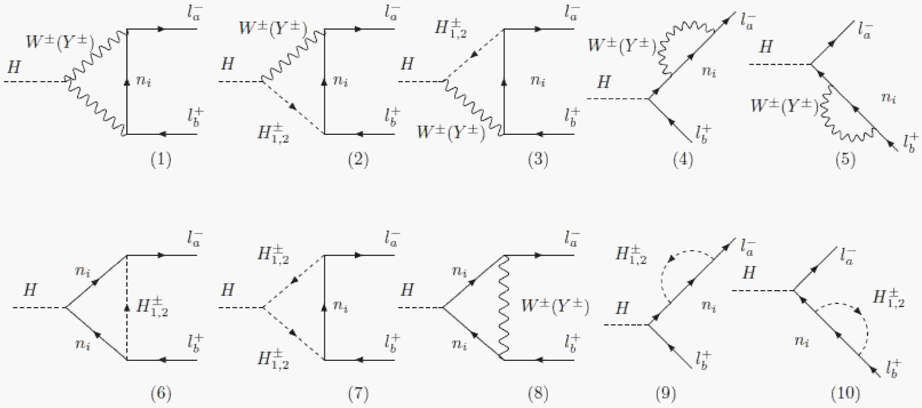
In this section, we focus on the lepton-flavor-violating decays $ (l_a \rightarrow l_b\gamma) $ and $ (H \rightarrow l_al_b),\, H\equiv h_1,\,h_2 $. These channels are closely related because they share a common source of lepton-flavor violation. Based on existing experimental constraints, we identify suitable regions of the model parameter space in which interesting phenomenology and signatures of new physics may arise.

In this section, we focus on the lepton-flavor-violating decays $ (l_a \rightarrow l_b\gamma) $ and $ (H \rightarrow l_al_b),\, H\equiv h_1,\,h_2 $. These channels are closely related because they share a common source of lepton-flavor violation. Based on existing experimental constraints, we identify suitable regions of the model parameter space in which interesting phenomenology and signatures of new physics may arise.

All lepton-flavor-violating interactions can be derived from the Lagrangian given in Eq. (9). We rewrite them in a convenient form as follows:

The lepton mass-mixing matrices are given by

with the corresponding assignment:

and

Substituting these expressions into Eq. (48), we obtain the corresponding results for the first and second terms on the right-hand side:

In Eq. (52), we used the supset ($ \supset $) notation to indicate the omission of irrelevant interactions that arise when transforming from the interaction basis to the physical basis. The remaining terms are couplings relevant to LFV processes.

In agreement with current experimental observations, charged leptons are assumed not to oscillate, and active neutrinos acquire masses through a type-I seesaw mechanism. We define the transformations between the flavor basis $ \{l'_{aL,R}\} $, $ \left\lbrace n'_i\right\rbrace =\{\nu'_{aL},\; (N'_{aR})^C\}) $ and the mass basis $ \{l_{aL,R}\} $, $ \left\lbrace n_i\right\rbrace =\{\nu_{aL},\; (N_{aR})^C\} $:

where $ M^D_\nu $ and $ M_N $ have the same form as in Eq. (50).

From the above expansions, we present the lepton-flavor-violating couplings of this model in Table 2,

where

In the framework of 331ALP, there are no trilinear couplings of the form $ l_a\overline{l}_b\gamma $ ($ a\neq b $). This can be verified directly from the kinetic term, $ {\cal{L}}^{kin}_{Lepton}=-{\rm i}\bar{\psi}_{aL}D /_\mu \psi_{aL} $. Therefore, the decays $ (l_a \rightarrow l_b\gamma) $ arise only at the loop level. Based on Table 2, we determine that the particles contributing to the loops in these decays can be the following: $ (\nu_a,W^\pm) $, $ (\nu_a,V^\pm) $, $ (\nu_a,H^\pm_{1,2}) $, and $ (N_a,H_1^\pm) $. The left- and right-handed components of the amplitude for $ (l_a \rightarrow l_b\gamma) $ are expressed in terms of the PV functions given in Appendix B.

The total branching ratios of the cLFV processes can be written based on Refs. [22, 29, 50, 51] in the form:

where $ G_F=g^2/(4\sqrt{2}m_W^2) $. For decays of different charged leptons, we use the experimental data $ {\rm{Br}}(\mu\rightarrow e\overline{\nu_e}\nu_\mu)=$100%, $ {\rm{Br}}(\tau\rightarrow e\overline{\nu_e}\nu_\tau)= $17.82%, $ {\rm{Br}}(\tau\rightarrow \mu\overline{\nu_\mu}\nu_\tau)= $17.39% given in Refs.[4, 5, 8].

The couplings in Table 2 are determined by the characteristics of the model under consideration. Therefore, we obtain the following interesting results: i) $ \bar{N}_{a} l_bH_2^{+}=0 $ implies that diagram 6) receives contributions only from $ H_1^\pm $, ii) $ N_a $ does not interact with charged gauge bosons, so diagram 8) gives no contribution in either the $ h_1 $ or $ h_2 $ case. Therefore, all one-loop Feynman diagrams for the decays $ H\rightarrow l_al_b,\,\,(H\equiv h_1,\,h_2) $ are shown in Fig. 1, and the corresponding amplitudes are presented in appendix B.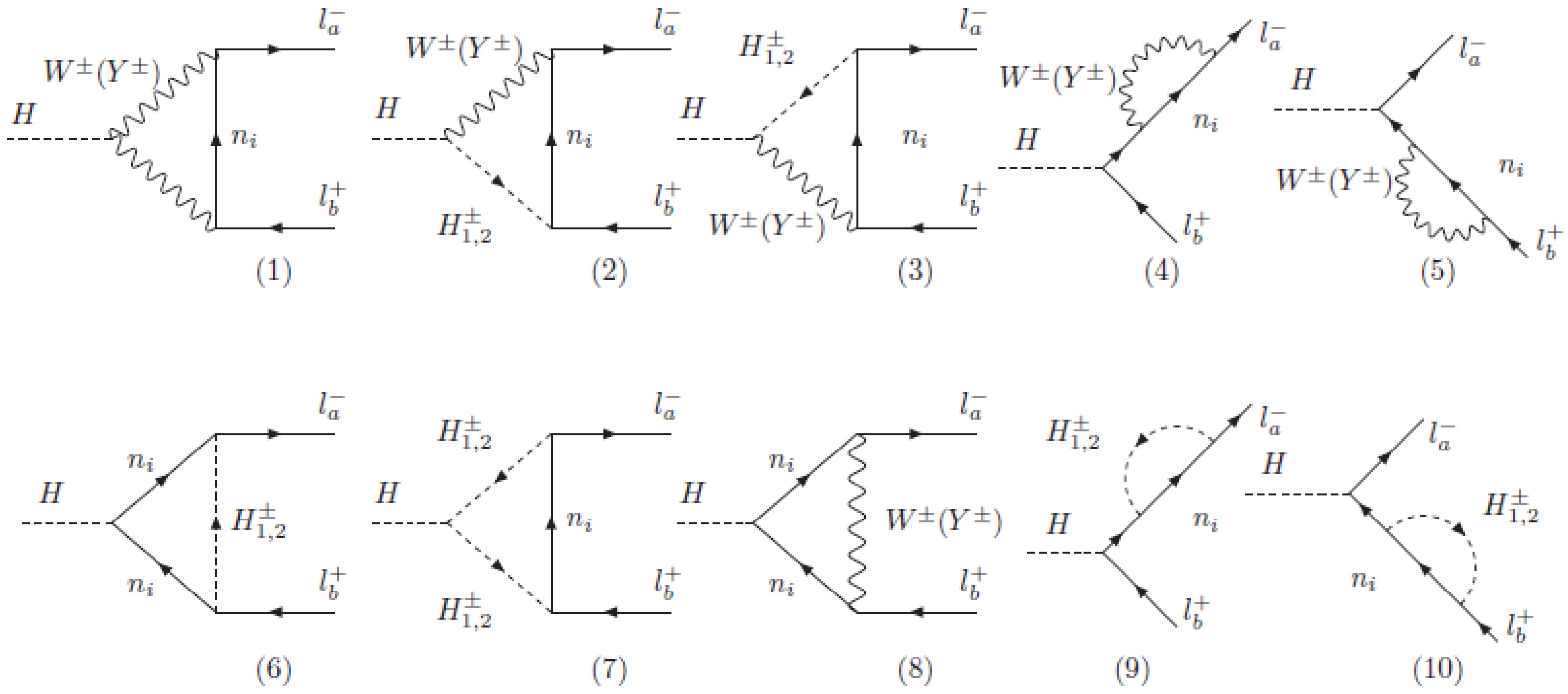

Figure 1.  Feynman diagrams at one-loop order for the decays $ H \rightarrow l_a l_b $ in the unitary gauge, where $ H \equiv \{h_1, h_2\}. $

The partial width of $ {\rm{H}}\rightarrow l_a^{\pm}l_b^{\mp} $ is

We impose the following conditions on the external momenta: $ p^2_{a,b}=m^2_{a,b} $, $ (p_a+p_b)^2=m^2_{{\rm{H}}} $, and $ m^2_{{\rm{H}}}\gg m^2_{a,b} $. Under these conditions, the branching ratio for the decay $ {\rm{H}}\rightarrow l_a^{\pm}l_b^{\mp} $ is given by

We need to determine $ \Gamma^{\rm{total}}_{{\rm{H}}} $, which can be constrained using current experimental data on the SM Higgs boson [52]. Its main contributions are

We focus on the SM Higgs boson with a mass of $ 125.09\; \; {\rm{GeV}} $. The branching ratios for the channels in Eq. (59) are given in Table 3 [53], and the total decay width ($ \Gamma^{\rm{SM}}_h $) is approximately $ 4.1\times 10^{-3}\; {\rm{GeV}} $ [54, 55].

For the CP-even Higgs bosons of the BSM, we can estimate $ \Gamma^{\rm{total}}_{{\rm{H}}} $ using a method similar to that presented in Ref.[56]. Accordingly, the partial decay width for each channel in Eq. (59) is determined from the branching ratios in Table 3, combined with a comparison to the corresponding quantity in the SM. Applying this procedure to the case $ H\equiv h_1,\; h_2 $ in this model, we present the couplings of H to quarks relevant to Eq. (59), based on Eq. (9), in Table 4.

Then, the partial decay widths of the first five channels in Eq. (59) are obtained from a combination of the branching ratios in Table 3 and the couplings in Tables 2 and 4. The last two channels in Eq. (59) are assumed to have the same branching ratios as in the SM. The total decay width is

where $ G\equiv W^\pm,\; Z $, $ H\equiv h_1,\; h_2 $, and $ f\equiv \tau, b, c $.

The last three terms in Eq. (60) are loop-induced decays in the SM. However, since $ h_{1,2} $ do not interact with exotic quarks, $ \Gamma ({\rm{H}}\rightarrow gg)\simeq \Gamma ({\rm{H}}\rightarrow \overline{u_3}u_3),\; u_3 \equiv t $ quark. The remaining two terms are given as

By substituting Eq. (61) into Eq. (60) and combining the result with Table 3 and Table 4, we can determine the total decay widths of $ h_1 $ and $ h_2 $. Note that in Eq. (60), $ \Gamma^{\rm{SM}}_{h}\simeq 4.1\times 10^{-3}\; {\rm{GeV}} $ corresponds to $ m_{h}=125.09\;{\rm{GeV}} $ [54−56], and the current experimental upper bound on $ {\rm{Br}}({\rm{h}} \rightarrow \mu \tau) $ is $ 10^{-3} $, as shown in Refs. [4, 5, 8].

All lepton-flavor-violating interactions can be derived from the Lagrangian given in Eq. (9). We rewrite them in a convenient form as follows:

The lepton mass-mixing matrices are given by

with the corresponding assignment:

and

Substituting these expressions into Eq. (48), we obtain the corresponding results for the first and second terms on the right-hand side:

In Eq. (52), we used the supset ($ \supset $) notation to indicate the omission of irrelevant interactions that arise when transforming from the interaction basis to the physical basis. The remaining terms are couplings relevant to LFV processes.

In agreement with current experimental observations, charged leptons are assumed not to oscillate, and active neutrinos acquire masses through a type-I seesaw mechanism. We define the transformations between the flavor basis $ \{l'_{aL,R}\} $, $ \left\lbrace n'_i\right\rbrace =\{\nu'_{aL},\; (N'_{aR})^C\}) $ and the mass basis $ \{l_{aL,R}\} $, $ \left\lbrace n_i\right\rbrace =\{\nu_{aL},\; (N_{aR})^C\} $:

where $ M^D_\nu $ and $ M_N $ have the same form as in Eq. (50).

From the above expansions, we present the lepton-flavor-violating couplings of this model in Table 2,

where

In the framework of 331ALP, there are no trilinear couplings of the form $ l_a\overline{l}_b\gamma $ ($ a\neq b $). This can be verified directly from the kinetic term, $ {\cal{L}}^{kin}_{Lepton}=-{\rm i}\bar{\psi}_{aL}D /_\mu \psi_{aL} $. Therefore, the decays $ (l_a \rightarrow l_b\gamma) $ arise only at the loop level. Based on Table 2, we determine that the particles contributing to the loops in these decays can be the following: $ (\nu_a,W^\pm) $, $ (\nu_a,V^\pm) $, $ (\nu_a,H^\pm_{1,2}) $, and $ (N_a,H_1^\pm) $. The left- and right-handed components of the amplitude for $ (l_a \rightarrow l_b\gamma) $ are expressed in terms of the PV functions given in Appendix B.

The total branching ratios of the cLFV processes can be written based on Refs. [22, 29, 50, 51] in the form:

where $ G_F=g^2/(4\sqrt{2}m_W^2) $. For decays of different charged leptons, we use the experimental data $ {\rm{Br}}(\mu\rightarrow e\overline{\nu_e}\nu_\mu)=$100%, $ {\rm{Br}}(\tau\rightarrow e\overline{\nu_e}\nu_\tau)= $17.82%, $ {\rm{Br}}(\tau\rightarrow \mu\overline{\nu_\mu}\nu_\tau)= $17.39% given in Refs.[4, 5, 8].

The couplings in Table 2 are determined by the characteristics of the model under consideration. Therefore, we obtain the following interesting results: i) $ \bar{N}_{a} l_bH_2^{+}=0 $ implies that diagram 6) receives contributions only from $ H_1^\pm $, ii) $ N_a $ does not interact with charged gauge bosons, so diagram 8) gives no contribution in either the $ h_1 $ or $ h_2 $ case. Therefore, all one-loop Feynman diagrams for the decays $ H\rightarrow l_al_b,\,\,(H\equiv h_1,\,h_2) $ are shown in Fig. 1, and the corresponding amplitudes are presented in appendix B.

Figure 1.  Feynman diagrams at one-loop order for the decays $ H \rightarrow l_a l_b $ in the unitary gauge, where $ H \equiv \{h_1, h_2\}. $

The partial width of $ {\rm{H}}\rightarrow l_a^{\pm}l_b^{\mp} $ is

We impose the following conditions on the external momenta: $ p^2_{a,b}=m^2_{a,b} $, $ (p_a+p_b)^2=m^2_{{\rm{H}}} $, and $ m^2_{{\rm{H}}}\gg m^2_{a,b} $. Under these conditions, the branching ratio for the decay $ {\rm{H}}\rightarrow l_a^{\pm}l_b^{\mp} $ is given by

We need to determine $ \Gamma^{\rm{total}}_{{\rm{H}}} $, which can be constrained using current experimental data on the SM Higgs boson [52]. Its main contributions are

We focus on the SM Higgs boson with a mass of $ 125.09\; \; {\rm{GeV}} $. The branching ratios for the channels in Eq. (59) are given in Table 3 [53], and the total decay width ($ \Gamma^{\rm{SM}}_h $) is approximately $ 4.1\times 10^{-3}\; {\rm{GeV}} $ [54, 55].

For the CP-even Higgs bosons of the BSM, we can estimate $ \Gamma^{\rm{total}}_{{\rm{H}}} $ using a method similar to that presented in Ref.[56]. Accordingly, the partial decay width for each channel in Eq. (59) is determined from the branching ratios in Table 3, combined with a comparison to the corresponding quantity in the SM. Applying this procedure to the case $ H\equiv h_1,\; h_2 $ in this model, we present the couplings of H to quarks relevant to Eq. (59), based on Eq. (9), in Table 4.

Then, the partial decay widths of the first five channels in Eq. (59) are obtained from a combination of the branching ratios in Table 3 and the couplings in Tables 2 and 4. The last two channels in Eq. (59) are assumed to have the same branching ratios as in the SM. The total decay width is

where $ G\equiv W^\pm,\; Z $, $ H\equiv h_1,\; h_2 $, and $ f\equiv \tau, b, c $.

The last three terms in Eq. (60) are loop-induced decays in the SM. However, since $ h_{1,2} $ do not interact with exotic quarks, $ \Gamma ({\rm{H}}\rightarrow gg)\simeq \Gamma ({\rm{H}}\rightarrow \overline{u_3}u_3),\; u_3 \equiv t $ quark. The remaining two terms are given as

By substituting Eq. (61) into Eq. (60) and combining the result with Table 3 and Table 4, we can determine the total decay widths of $ h_1 $ and $ h_2 $. Note that in Eq. (60), $ \Gamma^{\rm{SM}}_{h}\simeq 4.1\times 10^{-3}\; {\rm{GeV}} $ corresponds to $ m_{h}=125.09\;{\rm{GeV}} $ [54−56], and the current experimental upper bound on $ {\rm{Br}}({\rm{h}} \rightarrow \mu \tau) $ is $ 10^{-3} $, as shown in Refs. [4, 5, 8].

We use the well-established experimental parameters [4, 8]: the charged-lepton masses $ m_e=5\times 10^{-4}\,{\rm{GeV}} $, $ m_\mu= 0.105\,{\rm{GeV}} $, and $ m_\tau=1.776\,{\rm{GeV}} $; the SM-like Higgs mass $ m_{h}=125.1\,{\rm{GeV}} $; the W-boson mass $ m_W=80.385\,{\rm{GeV}} $; the $ S U(2)_L $ gauge coupling $ g \simeq 0.651 $; and $ v=246\,{\rm{GeV}} $. The mixing angles are treated as both free and dependent parameters, as specified below, to investigate the numerical behavior of the LFV process. However, this analysis is challenging because of the large number of parameters. This issue can be addressed by choosing $ t_\alpha $ and $ m_{H^\pm_2} $ as free parameters. In particular, $ t_{\alpha_2} $ can be expressed as a dependent parameter in terms of $ t_{\alpha_3} $, $ t_{\alpha_\phi} $, and the $ {\rm{VeVs}} $ using the relations in Eq. (40).

where the VEVs are expressed in terms of other parameters, such as the mass of the new charged gauge boson ($ m_Y^\pm $) and the mixing angle α ($ t_\alpha=\dfrac{v_\eta}{v_\rho} $). In particular, $ v_{\chi }=\sqrt{\dfrac{4m_Y^2}{g^2}-v_\rho^2},\, v_{\eta }=\dfrac{v t_a}{\sqrt{t_a^2+1}},\, v_{\rho }=\dfrac{v}{\sqrt{t_a^2+1}} $. The $ \sin{\phi_i} $ and $ \cos{\phi_i} $ functions of arbitrary angles $ \phi_i $ can be related to $ \tan{\phi_i} $ through the formulas $s_{\phi_i}= \dfrac{t_{\phi_i}}{\sqrt{t_{\phi_i}^2+1}}$, $ c_{\phi_i}=\dfrac{1}{\sqrt{t_{\phi_i}^2+1}} $. Furthermore, the Yukawa couplings and scalar self-coupling constants are chosen to be smaller than $ \sqrt{4\pi} $ and $ 4\pi $, respectively, in order to satisfy the perturbativity limits (Ref. [52]).

Moreover, based on Eqs. (30), (40), the interaction constants are chosen as dependent parameters, whereas the remaining ones are treated as free parameters and must lie within ranges that satisfy the perturbativity limits ($ \lambda_i \leq 4\pi $). These dependent parameters are listed in Eq. (63).

To numerically investigate $ l_a \rightarrow l_b\gamma $ and the LFVHDs, we next consider the parametrization of the neutrino mixing matrix $ U^\nu $, starting from the original relation in the seesaw mechanism. It reads:

Using the neutrino oscillation data reported in Refs. [4−6, 8, 57], namely $ s^2_{12}=0.307,\; s^2_{23}=0.558, \; s^2_{13}=0.0219, \Delta m^2_{21}= 7.53\times 10^{-5}\;{\rm{ eV^2}}, \; \Delta m^2_{32}= 2.455\times 10^{-3}\; {\rm{eV^2}} $, and choosing the Dirac and Majorana phases of $ U_{\rm PMNS} $ in their simplest form (Refs. [16, 51, 58]), we can determine the right-hand side of Eq. (65) in a known form. Furthermore, $ M_\nu^D $ must be antisymmetric; therefore, it contains only six unknowns. Together with $ M_N $ in diagonal form, this gives three additional unknowns. Hence, there are nine unknowns in total on the right-hand side, so Eq. (65) can be solved. This means that we have successfully parametrized $ U^\nu $.

We investigate the numerical results for $ l_a \rightarrow l_b\gamma $ in the parameter space $ 10^{-3}\leq t_\alpha \leq 10^3 $ and $ 300\leq m^\pm_{H_2} \leq 5 \times 10^3\, {\rm{GeV}} $. We find that $ \tau \rightarrow e\gamma $ is always below the experimental limit ($ 4.4 \times 10^{-8} $). The region of parameter space exceeding the upper limit for $ \tau \rightarrow \mu\gamma $ is indicated in green, with pink dashed lines corresponding to $ {\rm{Br}}(\tau \rightarrow \mu\gamma)=3.3\times 10^{-8} $ and $ 15\times 10^{-8} $. Meanwhile, the yellow and blue markers represent the parameter space in which $ {\rm{Br}}(\mu \rightarrow e\gamma) $ takes values above the upper bound. The curves corresponding to $ {\rm{Br}}(\mu \rightarrow e\gamma)= 4.2\times 10^{-13} $ and $ 10\times 10^{-13} $ can also be found there. Therefore, the region allowed by the experimental constraints on $ l_a \rightarrow l_b\gamma $ decays is the uncolored part in Fig. 2.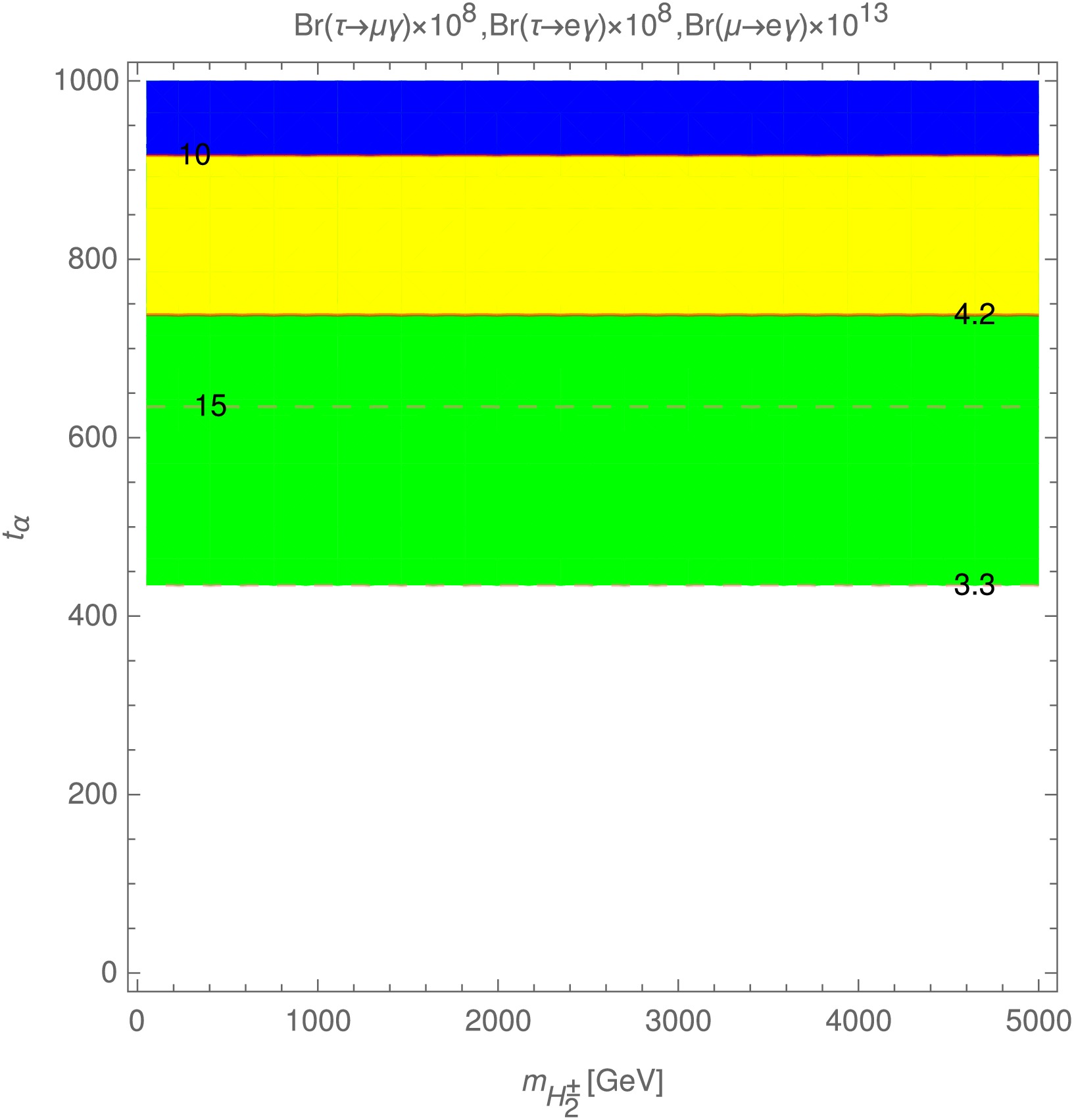

Figure 2.  (color online) Contour plots of $ l_a \rightarrow l_b\gamma $ decays in the plane of ($ t_\alpha, m_{H^\pm_2} $).

Based on the analytical expressions for the amplitudes given in appendix B, we investigate the values of $ {\rm{Br}}(h_1 \rightarrow \mu \tau) $ and $ {\rm{Br}}(h_2 \rightarrow \mu \tau) $, which are shown in Fig. 3. We observe that most of the values of $ {\rm{Br}}(h_1 \rightarrow \mu \tau) $ in the left panel and $ {\rm{Br}}(h_2 \rightarrow \mu \tau) $ in the right panel lie within the current experimental limits ($ \leq 10^{-3} $).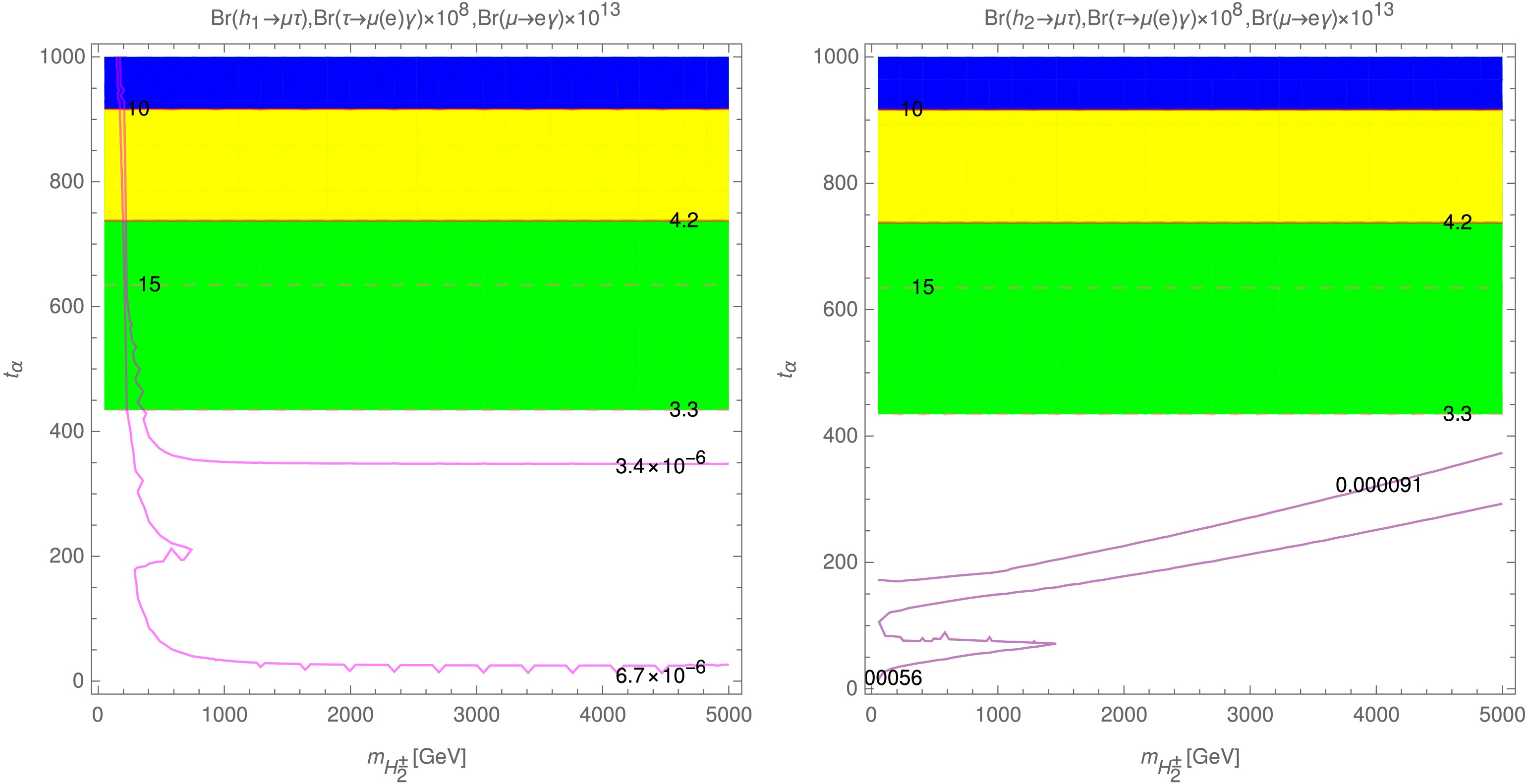

Figure 3.  (color online) Plots of $ {\rm{Br}}(h_1 \rightarrow \mu \tau) $ (left panel) and $ {\rm{Br}}(h_2 \rightarrow \mu \tau) $ (right panel) in the ($ t_\alpha, m_{H^\pm_2} $) plane.

To illustrate this, we present the signals of $ {\rm{Br}}(h_1 \rightarrow \mu \tau) $ and $ {\rm{Br}}(h_2 \rightarrow \mu \tau) $ in the allowed parameter-space region in Fig. 3. In the left panel of Fig. 3, $ {\rm{Br}}(h_1 \rightarrow \mu \tau) $ can reach values of $ 3.4 \times 10^{-6} $ and $ 6.7 \times 10^{-6} $, while in the right panel, $ {\rm{Br}}(h_2 \rightarrow \mu \tau) $ can reach values of $ 9.1 \times 10^{-5} $ and $ 5.6 \times 10^{-5} $. All of these values satisfy the current experimental limits.

Next, we predict the mass of the new CP-even Higgs boson based on gluon-gluon fusion at the LHC and the CMS data analysis. The Higgs-boson production signal in proton-proton collisions is modeled under the assumption of a narrow Higgs-boson width [59]. In this case, the partons can be gluons or quarks [60, 61]. Therefore, the hadronic cross section depends on the parton luminosity and the partonic cross section as follows [60, 61]

where g and q denote gluons and quarks, respectively.

As shown in Eq. (66), Higgs boson production in proton-proton collisions at the LHC involves partons, namely gluons and quarks. However, because of their relatively large masses, the densities of quarks inside the proton are significantly lower than that of gluons. Consequently, the gluon parton distribution plays the dominant role in Higgs production, with the gluons eventually coupling through a quark loop. Therefore, we approximate the hadronic cross section by considering only gluon-initiated partons, which takes the form [62, 63]

The parton luminosity is related to the parton distribution function as

where $ F_{g}\left(x, m_H^2 \right) $ is the gluon parton distribution function, $ \sqrt{s} $ is the center-of-mass energy of the collider, and $ \hat{\sigma} $ is the partonic cross section, expanded in terms of the strong coupling constant ($ \alpha_s $), as follows Refs. [60, 61]:

Loop corrections involving intermediate quarks are the primary source of Higgs boson production via gluon-gluon fusion. However, the t-quark provides the dominant contribution to this process, because the Higgs boson couples about 35 times more strongly to the t-quark than to the next-heaviest fermion, the b-quark. Consequently, the other contributions can be neglected, and only the t-quark contribution needs to be considered. Thus, the leading-order approximation in Eq.(69) is expressed as follows [60, 64]:

where $ G_{\rm F} $ is the Fermi constant, $ \zeta=\dfrac{4m^2_t}{m^2_H} $, $ m_t $ is t-quark mass and

For dilepton decays, if the decay width is assumed to be very narrow, the cross section of these processes can be approximated as

By analyzing data at a center-of-mass energy of 13 $ {\rm{TeV}} $ and an integrated luminosity of $ 35.9\; {\rm{fb}}^{-1} $, CMS has shown that $ \sigma \left(gg \rightarrow H \right) \times {\rm{Br}} \left(H \rightarrow \mu\tau \right) $ can range from $ 51.9\; (57.4)\; {\rm{fb}} $ to $ 1.6 \; (2.1)\; {\rm{fb}} $ at the 95% confidence level [38]. To optimize the analysis of the experimental data, CMS divided the mass range into two regions: a low-mass region of 200–450 $ {\rm{GeV}} $ and a high-mass region of 450–900 $ {\rm{GeV}} $.

As results, we present the combined processes $ \sigma \left(gg \rightarrow H \right) \times {\rm{Br}} \left(H \rightarrow \mu\tau_h \right) $ and $ \sigma \left(gg \rightarrow H \right) \times {\rm{Br}} \left(H \rightarrow \mu\tau_e \right) $ at 95% CL as the green and cyan lines, respectively, in Fig. 4. The dotted black line represents the boundary between the two mass scales.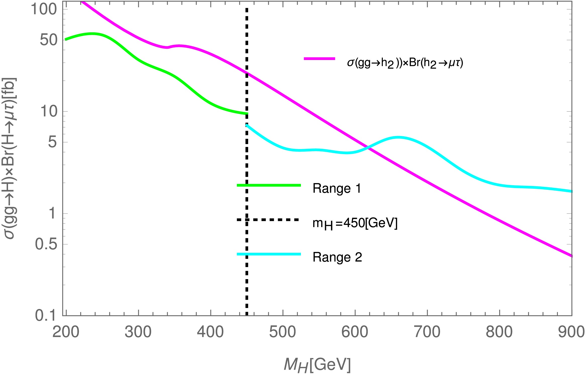

Figure 4.  (color online) Plots of $ \sigma \left(gg \rightarrow h_2 \right) \times {\rm{Br}} \left(h_2 \rightarrow \mu\tau \right) $ (magenta line) as functions of $ M_H $ are shown, while the green and cyan lines represent the CMS observations for the combined decay modes of $ H \rightarrow \mu\tau $ (based on Ref. [38]) in the low- and high-mass ranges, respectively.

To predict the masses of the new CP-even Higgs bosons, $ h_2 $, the parton distribution functions are chosen in a non-relativistic form (Breit-Wigner distribution functions), and the partonic cross section is approximated at leading order. For simplicity, $ \hat{\sigma}\left(gg \rightarrow H \right)\sim \dfrac{G_Fm^2_H \zeta^2}{\sqrt{2}\pi} \left| 1+(1-\zeta)f(\zeta)\right| ^2 $. Therefore, we investigate the signal $ \sigma \left(gg \rightarrow h^0_2 \right) \times {\rm{Br}} \left(h^0_2 \rightarrow \mu\tau \right) $, shown as the magenta line in Fig. 4, and the mass of $ h_2 $ is predicted to be greater than $ 630 \; {\rm{GeV}} $.

We use the well-established experimental parameters [4, 8]: the charged-lepton masses $ m_e=5\times 10^{-4}\,{\rm{GeV}} $, $ m_\mu= 0.105\,{\rm{GeV}} $, and $ m_\tau=1.776\,{\rm{GeV}} $; the SM-like Higgs mass $ m_{h}=125.1\,{\rm{GeV}} $; the W-boson mass $ m_W=80.385\,{\rm{GeV}} $; the $ S U(2)_L $ gauge coupling $ g \simeq 0.651 $; and $ v=246\,{\rm{GeV}} $. The mixing angles are treated as both free and dependent parameters, as specified below, to investigate the numerical behavior of the LFV process. However, this analysis is challenging because of the large number of parameters. This issue can be addressed by choosing $ t_\alpha $ and $ m_{H^\pm_2} $ as free parameters. In particular, $ t_{\alpha_2} $ can be expressed as a dependent parameter in terms of $ t_{\alpha_3} $, $ t_{\alpha_\phi} $, and the $ {\rm{VeVs}} $ using the relations in Eq. (40).

where the VEVs are expressed in terms of other parameters, such as the mass of the new charged gauge boson ($ m_Y^\pm $) and the mixing angle α ($ t_\alpha=\dfrac{v_\eta}{v_\rho} $). In particular, $ v_{\chi }=\sqrt{\dfrac{4m_Y^2}{g^2}-v_\rho^2},\, v_{\eta }=\dfrac{v t_a}{\sqrt{t_a^2+1}},\, v_{\rho }=\dfrac{v}{\sqrt{t_a^2+1}} $. The $ \sin{\phi_i} $ and $ \cos{\phi_i} $ functions of arbitrary angles $ \phi_i $ can be related to $ \tan{\phi_i} $ through the formulas $s_{\phi_i}= \dfrac{t_{\phi_i}}{\sqrt{t_{\phi_i}^2+1}}$, $ c_{\phi_i}=\dfrac{1}{\sqrt{t_{\phi_i}^2+1}} $. Furthermore, the Yukawa couplings and scalar self-coupling constants are chosen to be smaller than $ \sqrt{4\pi} $ and $ 4\pi $, respectively, in order to satisfy the perturbativity limits (Ref. [52]).

Moreover, based on Eqs. (30), (40), the interaction constants are chosen as dependent parameters, whereas the remaining ones are treated as free parameters and must lie within ranges that satisfy the perturbativity limits ($ \lambda_i \leq 4\pi $). These dependent parameters are listed in Eq. (63).

To numerically investigate $ l_a \rightarrow l_b\gamma $ and the LFVHDs, we next consider the parametrization of the neutrino mixing matrix $ U^\nu $, starting from the original relation in the seesaw mechanism. It reads:

Using the neutrino oscillation data reported in Refs. [4−6, 8, 57], namely $ s^2_{12}=0.307,\; s^2_{23}=0.558, \; s^2_{13}=0.0219, \Delta m^2_{21}= 7.53\times 10^{-5}\;{\rm{ eV^2}}, \; \Delta m^2_{32}= 2.455\times 10^{-3}\; {\rm{eV^2}} $, and choosing the Dirac and Majorana phases of $ U_{\rm PMNS} $ in their simplest form (Refs. [16, 51, 58]), we can determine the right-hand side of Eq. (65) in a known form. Furthermore, $ M_\nu^D $ must be antisymmetric; therefore, it contains only six unknowns. Together with $ M_N $ in diagonal form, this gives three additional unknowns. Hence, there are nine unknowns in total on the right-hand side, so Eq. (65) can be solved. This means that we have successfully parametrized $ U^\nu $.

We investigate the numerical results for $ l_a \rightarrow l_b\gamma $ in the parameter space $ 10^{-3}\leq t_\alpha \leq 10^3 $ and $ 300\leq m^\pm_{H_2} \leq 5 \times 10^3\, {\rm{GeV}} $. We find that $ \tau \rightarrow e\gamma $ is always below the experimental limit ($ 4.4 \times 10^{-8} $). The region of parameter space exceeding the upper limit for $ \tau \rightarrow \mu\gamma $ is indicated in green, with pink dashed lines corresponding to $ {\rm{Br}}(\tau \rightarrow \mu\gamma)=3.3\times 10^{-8} $ and $ 15\times 10^{-8} $. Meanwhile, the yellow and blue markers represent the parameter space in which $ {\rm{Br}}(\mu \rightarrow e\gamma) $ takes values above the upper bound. The curves corresponding to $ {\rm{Br}}(\mu \rightarrow e\gamma)= 4.2\times 10^{-13} $ and $ 10\times 10^{-13} $ can also be found there. Therefore, the region allowed by the experimental constraints on $ l_a \rightarrow l_b\gamma $ decays is the uncolored part in Fig. 2.

Figure 2.  (color online) Contour plots of $ l_a \rightarrow l_b\gamma $ decays in the plane of ($ t_\alpha, m_{H^\pm_2} $).

Based on the analytical expressions for the amplitudes given in appendix B, we investigate the values of $ {\rm{Br}}(h_1 \rightarrow \mu \tau) $ and $ {\rm{Br}}(h_2 \rightarrow \mu \tau) $, which are shown in Fig. 3. We observe that most of the values of $ {\rm{Br}}(h_1 \rightarrow \mu \tau) $ in the left panel and $ {\rm{Br}}(h_2 \rightarrow \mu \tau) $ in the right panel lie within the current experimental limits ($ \leq 10^{-3} $).

Figure 3.  (color online) Plots of $ {\rm{Br}}(h_1 \rightarrow \mu \tau) $ (left panel) and $ {\rm{Br}}(h_2 \rightarrow \mu \tau) $ (right panel) in the ($ t_\alpha, m_{H^\pm_2} $) plane.

To illustrate this, we present the signals of $ {\rm{Br}}(h_1 \rightarrow \mu \tau) $ and $ {\rm{Br}}(h_2 \rightarrow \mu \tau) $ in the allowed parameter-space region in Fig. 3. In the left panel of Fig. 3, $ {\rm{Br}}(h_1 \rightarrow \mu \tau) $ can reach values of $ 3.4 \times 10^{-6} $ and $ 6.7 \times 10^{-6} $, while in the right panel, $ {\rm{Br}}(h_2 \rightarrow \mu \tau) $ can reach values of $ 9.1 \times 10^{-5} $ and $ 5.6 \times 10^{-5} $. All of these values satisfy the current experimental limits.

Next, we predict the mass of the new CP-even Higgs boson based on gluon-gluon fusion at the LHC and the CMS data analysis. The Higgs-boson production signal in proton-proton collisions is modeled under the assumption of a narrow Higgs-boson width [59]. In this case, the partons can be gluons or quarks [60, 61]. Therefore, the hadronic cross section depends on the parton luminosity and the partonic cross section as follows [60, 61]

where g and q denote gluons and quarks, respectively.

As shown in Eq. (66), Higgs boson production in proton-proton collisions at the LHC involves partons, namely gluons and quarks. However, because of their relatively large masses, the densities of quarks inside the proton are significantly lower than that of gluons. Consequently, the gluon parton distribution plays the dominant role in Higgs production, with the gluons eventually coupling through a quark loop. Therefore, we approximate the hadronic cross section by considering only gluon-initiated partons, which takes the form [62, 63]

The parton luminosity is related to the parton distribution function as

where $ F_{g}\left(x, m_H^2 \right) $ is the gluon parton distribution function, $ \sqrt{s} $ is the center-of-mass energy of the collider, and $ \hat{\sigma} $ is the partonic cross section, expanded in terms of the strong coupling constant ($ \alpha_s $), as follows Refs. [60, 61]:

Loop corrections involving intermediate quarks are the primary source of Higgs boson production via gluon-gluon fusion. However, the t-quark provides the dominant contribution to this process, because the Higgs boson couples about 35 times more strongly to the t-quark than to the next-heaviest fermion, the b-quark. Consequently, the other contributions can be neglected, and only the t-quark contribution needs to be considered. Thus, the leading-order approximation in Eq.(69) is expressed as follows [60, 64]:

where $ G_{\rm F} $ is the Fermi constant, $ \zeta=\dfrac{4m^2_t}{m^2_H} $, $ m_t $ is t-quark mass and

For dilepton decays, if the decay width is assumed to be very narrow, the cross section of these processes can be approximated as

By analyzing data at a center-of-mass energy of 13 $ {\rm{TeV}} $ and an integrated luminosity of $ 35.9\; {\rm{fb}}^{-1} $, CMS has shown that $ \sigma \left(gg \rightarrow H \right) \times {\rm{Br}} \left(H \rightarrow \mu\tau \right) $ can range from $ 51.9\; (57.4)\; {\rm{fb}} $ to $ 1.6 \; (2.1)\; {\rm{fb}} $ at the 95% confidence level [38]. To optimize the analysis of the experimental data, CMS divided the mass range into two regions: a low-mass region of 200–450 $ {\rm{GeV}} $ and a high-mass region of 450–900 $ {\rm{GeV}} $.

As results, we present the combined processes $ \sigma \left(gg \rightarrow H \right) \times {\rm{Br}} \left(H \rightarrow \mu\tau_h \right) $ and $ \sigma \left(gg \rightarrow H \right) \times {\rm{Br}} \left(H \rightarrow \mu\tau_e \right) $ at 95% CL as the green and cyan lines, respectively, in Fig. 4. The dotted black line represents the boundary between the two mass scales.

Figure 4.  (color online) Plots of $ \sigma \left(gg \rightarrow h_2 \right) \times {\rm{Br}} \left(h_2 \rightarrow \mu\tau \right) $ (magenta line) as functions of $ M_H $ are shown, while the green and cyan lines represent the CMS observations for the combined decay modes of $ H \rightarrow \mu\tau $ (based on Ref. [38]) in the low- and high-mass ranges, respectively.

To predict the masses of the new CP-even Higgs bosons, $ h_2 $, the parton distribution functions are chosen in a non-relativistic form (Breit-Wigner distribution functions), and the partonic cross section is approximated at leading order. For simplicity, $ \hat{\sigma}\left(gg \rightarrow H \right)\sim \dfrac{G_Fm^2_H \zeta^2}{\sqrt{2}\pi} \left| 1+(1-\zeta)f(\zeta)\right| ^2 $. Therefore, we investigate the signal $ \sigma \left(gg \rightarrow h^0_2 \right) \times {\rm{Br}} \left(h^0_2 \rightarrow \mu\tau \right) $, shown as the magenta line in Fig. 4, and the mass of $ h_2 $ is predicted to be greater than $ 630 \; {\rm{GeV}} $.

In 331ALP, the heavier neutral gauge boson, $ Z' $, has the mass and physical state given by Eq.(22) in section II. The interaction of $ Z' $ with fermions originates from the kinetic term of the spinor fields and has the following form:

where $ g_V^{Z^\prime} $ and $ g_A^{Z^\prime} $ are given in Table 5.

We also use the kinetic terms of the scalar fields, such as Eq. (13), to derive the non-zero couplings of $ Z^\prime $ to gauge and Higgs bosons, as shown in Table 6.

The LHC dilepton measurements at $ \sqrt{s}=13\; {\rm{TeV}} $ indicate that the cross section for the $ Z^{\prime} $-mediated process is given by the product of the hadronic cross section and the branching ratio [39]

where $ \xi_q $ and $ \overline{\xi}_q $ denote the parton distribution functions of quarks and antiquarks, respectively. The partonic cross section and branching ratio are given by:

where the final-state particles in the decay channel are dileptons. The corresponding decay width is given by Eq. (76), while the total decay width must also include the gauge and Higgs boson contributions, denoted by G and H, respectively, as listed in Eq. (77).

Because Z and $ Z^\prime $ do not mix, as shown in Eq. (22), $ \Gamma (Z^\prime \rightarrow W^+W^-) $ vanishes, according to Ref. [66]. Furthermore, since $ m_X \gt m_{Z^\prime}/2 $, $ \Gamma (Z^\prime \rightarrow X^*X,\; X \equiv V^\pm, X^{0*}, X^0 $ also does not contribute to the total width of $ Z^\prime $. The remaining components are given as follows [45, 65, 66]:

where $ E=\dfrac{m^2_{Z^\prime}+m^2_G-m^2_H}{2m_{Z^\prime}} $ denotes the energy of the final-state gauge boson, and the corresponding factors are taken from Tables 5 and 6.

Based on the analytical expressions in Eqs. (74), (75) and the known data given in Sec. IV, we show the dependence of $ \sigma \left(pp \rightarrow Z^\prime \rightarrow \overline{l}l \right) $ on $ m_{Z^\prime} $ as the blue line in Fig. 5. The red line depicts the upper limits on the dilepton production cross section reported by ATLAS at an integrated luminosity of $ 139\; {\rm{ fb^{-1}}} $ [7], while the black line is based on the 95% CL upper bound given by CMS at $ \sqrt{s}=13\; {\rm{TeV}} $ [39]. Therefore, to satisfy these constraints, we obtain $ m_{Z^\prime}\geqslant 5.1\; {\rm{TeV}} $; of course, for masses below this value, $ Z^\prime $ is excluded. The lower bound on the $ Z^\prime $ mass obtained in this work is highly consistent with non-supersymmetric models, such as $ Z^{\prime}_{\psi} $ in grand unified theories based on the $ E_6 $ gauge group or $ Z^{\prime}_{SSM} $ in the generalized sequential model [7, 39]. However, a major difference arises in supersymmetric models, where the lower bound on $ m_{Z^{\prime}} $, as mentioned above, is significantly smaller [67, 68].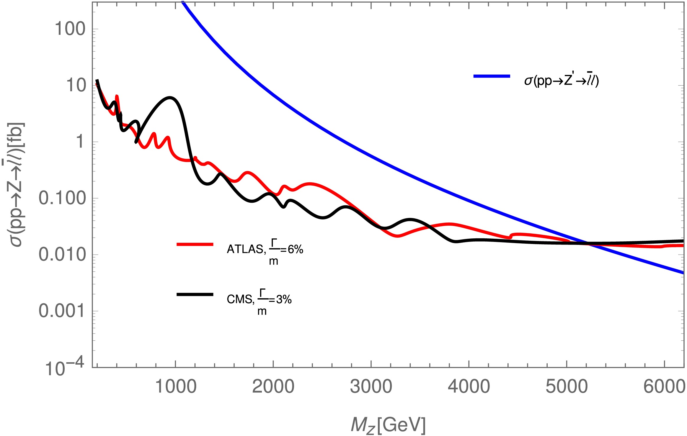

Figure 5.  (color online) The dependence of $ \sigma \left(pp \rightarrow Z^\prime \rightarrow \overline{l}l \right) $ on $ M_Z $ is shown by the blue line. The red line represents the ATLAS upper limits on the cross section for $ {\Gamma}/{m}= $6% [7]. The black line represents the CMS upper limits on the cross section for $ {\Gamma}/{m}= $3% at 95% CL [39].

In 331ALP, the heavier neutral gauge boson, $ Z' $, has the mass and physical state given by Eq.(22) in section II. The interaction of $ Z' $ with fermions originates from the kinetic term of the spinor fields and has the following form:

where $ g_V^{Z^\prime} $ and $ g_A^{Z^\prime} $ are given in Table 5.

We also use the kinetic terms of the scalar fields, such as Eq. (13), to derive the non-zero couplings of $ Z^\prime $ to gauge and Higgs bosons, as shown in Table 6.

The LHC dilepton measurements at $ \sqrt{s}=13\; {\rm{TeV}} $ indicate that the cross section for the $ Z^{\prime} $-mediated process is given by the product of the hadronic cross section and the branching ratio [39]

where $ \xi_q $ and $ \overline{\xi}_q $ denote the parton distribution functions of quarks and antiquarks, respectively. The partonic cross section and branching ratio are given by:

where the final-state particles in the decay channel are dileptons. The corresponding decay width is given by Eq. (76), while the total decay width must also include the gauge and Higgs boson contributions, denoted by G and H, respectively, as listed in Eq. (77).

Because Z and $ Z^\prime $ do not mix, as shown in Eq. (22), $ \Gamma (Z^\prime \rightarrow W^+W^-) $ vanishes, according to Ref. [66]. Furthermore, since $ m_X \gt m_{Z^\prime}/2 $, $ \Gamma (Z^\prime \rightarrow X^*X,\; X \equiv V^\pm, X^{0*}, X^0 $ also does not contribute to the total width of $ Z^\prime $. The remaining components are given as follows [45, 65, 66]:

where $ E=\dfrac{m^2_{Z^\prime}+m^2_G-m^2_H}{2m_{Z^\prime}} $ denotes the energy of the final-state gauge boson, and the corresponding factors are taken from Tables 5 and 6.

Based on the analytical expressions in Eqs. (74), (75) and the known data given in Sec. IV, we show the dependence of $ \sigma \left(pp \rightarrow Z^\prime \rightarrow \overline{l}l \right) $ on $ m_{Z^\prime} $ as the blue line in Fig. 5. The red line depicts the upper limits on the dilepton production cross section reported by ATLAS at an integrated luminosity of $ 139\; {\rm{ fb^{-1}}} $ [7], while the black line is based on the 95% CL upper bound given by CMS at $ \sqrt{s}=13\; {\rm{TeV}} $ [39]. Therefore, to satisfy these constraints, we obtain $ m_{Z^\prime}\geqslant 5.1\; {\rm{TeV}} $; of course, for masses below this value, $ Z^\prime $ is excluded. The lower bound on the $ Z^\prime $ mass obtained in this work is highly consistent with non-supersymmetric models, such as $ Z^{\prime}_{\psi} $ in grand unified theories based on the $ E_6 $ gauge group or $ Z^{\prime}_{SSM} $ in the generalized sequential model [7, 39]. However, a major difference arises in supersymmetric models, where the lower bound on $ m_{Z^{\prime}} $, as mentioned above, is significantly smaller [67, 68].

Figure 5.  (color online) The dependence of $ \sigma \left(pp \rightarrow Z^\prime \rightarrow \overline{l}l \right) $ on $ M_Z $ is shown by the blue line. The red line represents the ATLAS upper limits on the cross section for $ {\Gamma}/{m}= $6% [7]. The black line represents the CMS upper limits on the cross section for $ {\Gamma}/{m}= $3% at 95% CL [39].

From the symmetry-breaking scheme in (12), we see that $ Z_2 $ is the residual symmetry of the model; therefore, odd-$ Z_2 $ particles can be considered dark matter candidates. These include $ \eta,\,\rho,\,u_{aR},\,d_{nR},\,l_{aR},\,N_{aR} $, according to (7). However, η and ρ directly break the electroweak scale, and $ u_{aR},\,d_{nR},\,l_{aR} $ are components of ordinary matter; thus, only $ N_{aR} $ remains the most suitable dark matter candidate in the model.

Among $ N_{aR} $, we assume that $ N_{1R} $ is the lightest. Therefore, $ N_{1R} $ is identified as dark matter, and pairs of $ N_{1R} $ annihilate into SM particles in the early universe. Because $ N_{1R} $ interacts directly only with Φ according to Eq. (9), and Φ can couple to SM particles as in Eq. (27), the dominant contribution to dark matter annihilation mainly arises from s-channel exchange diagrams mediated by Φ. The corresponding diagram is shown in Fig. 6. Although Φ mixes with $ R_\chi $ and $ R_\phi $, and can therefore interact with fermions according to Eq. (46), the mixing angles are very small, as shown in Eq. (40). Therefore, the SM products of the dark matter pair annihilation channel do not include fermions, but only gauge bosons. This implies that $ N_{1R}^CN_{1R} \rightarrow h_1h_1,\; ZZ $. Hence, the product of the annihilation cross section of the dark matter pair and the relative velocity is approximately [39, 69]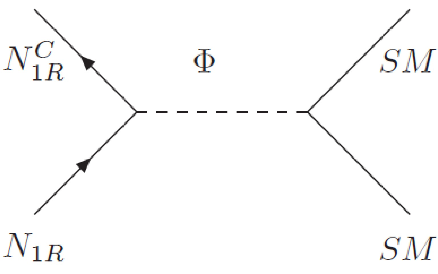

Figure 6.  Dominant contributions to dark matter annihilation.

where $ x_f\simeq 20.25 $ [70] and $ g_{\Phi N_{1R}^CN_{1R}}=\left(y_N \right)_{11} $, whereas $ g_{\Phi ZZ}=0 $ and $ g_{\Phi h_1h_1}=\dfrac{v_\phi}{2\sqrt{2}}\left(\lambda_{12} s_{ \alpha_2}^2+\lambda_{13} c_{ \alpha_2}^2 \right) $ are determined from Eq. (13) and Eq. (27), respectively.

We employed the dark matter relic abundance given in Ref. [71]:

We represent the dark matter relic density, $ 0.1\leq\Omega_{\rm DM} h^2 \leq 0.3 $ [72], in the ($ v_\Phi,\; m_{N_{1R}} $) plane, as shown in Fig. 7. We recall that, for the PQ symmetry not to be broken by quantum gravity effects and to ensure the emergence of a naturally light, stable axion, $ v_\phi\simeq 10^{11}\; \; {\rm{GeV}} $ (as mentioned in Sec. II). Therefore, $ v_\phi $ is taken to be the axion-breaking scale in the model. As a result, in Fig. 7, the colorless region corresponds to the parameter space consistent with current observations, in which there is a relationship between the dark matter mass and the axion-breaking scale.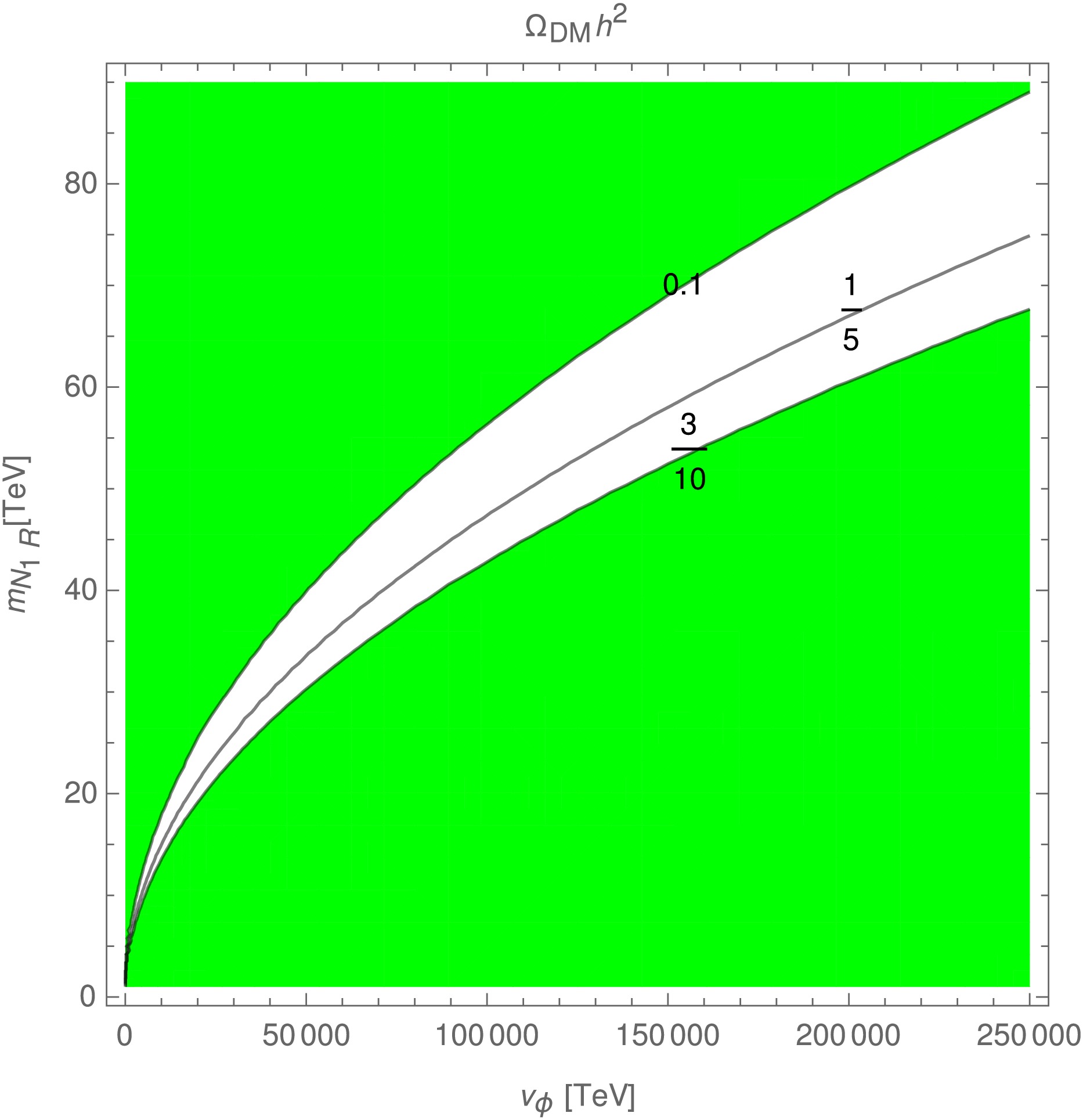

Figure 7.  (color online) Contours of the dark matter relic density in the ($ v_\Phi,\; m_{N_{1R}} $) plane.

From the symmetry-breaking scheme in (12), we see that $ Z_2 $ is the residual symmetry of the model; therefore, odd-$ Z_2 $ particles can be considered dark matter candidates. These include $ \eta,\,\rho,\,u_{aR},\,d_{nR},\,l_{aR},\,N_{aR} $, according to (7). However, η and ρ directly break the electroweak scale, and $ u_{aR},\,d_{nR},\,l_{aR} $ are components of ordinary matter; thus, only $ N_{aR} $ remains the most suitable dark matter candidate in the model.

Among $ N_{aR} $, we assume that $ N_{1R} $ is the lightest. Therefore, $ N_{1R} $ is identified as dark matter, and pairs of $ N_{1R} $ annihilate into SM particles in the early universe. Because $ N_{1R} $ interacts directly only with Φ according to Eq. (9), and Φ can couple to SM particles as in Eq. (27), the dominant contribution to dark matter annihilation mainly arises from s-channel exchange diagrams mediated by Φ. The corresponding diagram is shown in Fig. 6. Although Φ mixes with $ R_\chi $ and $ R_\phi $, and can therefore interact with fermions according to Eq. (46), the mixing angles are very small, as shown in Eq. (40). Therefore, the SM products of the dark matter pair annihilation channel do not include fermions, but only gauge bosons. This implies that $ N_{1R}^CN_{1R} \rightarrow h_1h_1,\; ZZ $. Hence, the product of the annihilation cross section of the dark matter pair and the relative velocity is approximately [39, 69]

Figure 6.  Dominant contributions to dark matter annihilation.

where $ x_f\simeq 20.25 $ [70] and $ g_{\Phi N_{1R}^CN_{1R}}=\left(y_N \right)_{11} $, whereas $ g_{\Phi ZZ}=0 $ and $ g_{\Phi h_1h_1}=\dfrac{v_\phi}{2\sqrt{2}}\left(\lambda_{12} s_{ \alpha_2}^2+\lambda_{13} c_{ \alpha_2}^2 \right) $ are determined from Eq. (13) and Eq. (27), respectively.

We employed the dark matter relic abundance given in Ref. [71]:

We represent the dark matter relic density, $ 0.1\leq\Omega_{\rm DM} h^2 \leq 0.3 $ [72], in the ($ v_\Phi,\; m_{N_{1R}} $) plane, as shown in Fig. 7. We recall that, for the PQ symmetry not to be broken by quantum gravity effects and to ensure the emergence of a naturally light, stable axion, $ v_\phi\simeq 10^{11}\; \; {\rm{GeV}} $ (as mentioned in Sec. II). Therefore, $ v_\phi $ is taken to be the axion-breaking scale in the model. As a result, in Fig. 7, the colorless region corresponds to the parameter space consistent with current observations, in which there is a relationship between the dark matter mass and the axion-breaking scale.

Figure 7.  (color online) Contours of the dark matter relic density in the ($ v_\Phi,\; m_{N_{1R}} $) plane.

In the 3-3-1 model with axionlike particles, we identify the region of parameter space in which both cLFV and LFVHD constraints satisfy the experimental limits. In these allowed regions, $ {\rm{Br}}(h_1 \rightarrow \mu\tau) $ is of the order of $ 10^{-6} $, while $ {\rm{Br}}(h_2 \rightarrow \mu\tau) $ reaches approximately $ 10^{-5} $. Based on gluon-gluon fusion at the LHC, we investigate the signal cross sections in the allowed parameter space and provide predictions for $ m_{h_2}\geq 630 \; {\rm{GeV}} $. Based on searches for high-mass dilepton resonances at ATLAS and CMS, we use the numerical result for $ \sigma \left(pp \rightarrow Z^\prime \rightarrow \overline{l}l \right) $ and show that the $ Z^\prime $-boson mass satisfies $ m_{Z^\prime}\geq 5.1 \; {\rm{TeV}} $. The hypothesis of the existence of a residual $ Z_2 $ symmetry after the stages of spontaneous symmetry breaking implies that only $ N_{aR} $ can be dark matter candidates among the odd-$ Z_2 $ particles. By investigating the dark matter relic density within experimentally allowed limits, we also establish a relationship between the dark matter mass and the axion breaking scale.

In the 3-3-1 model with axionlike particles, we identify the region of parameter space in which both cLFV and LFVHD constraints satisfy the experimental limits. In these allowed regions, $ {\rm{Br}}(h_1 \rightarrow \mu\tau) $ is of the order of $ 10^{-6} $, while $ {\rm{Br}}(h_2 \rightarrow \mu\tau) $ reaches approximately $ 10^{-5} $. Based on gluon-gluon fusion at the LHC, we investigate the signal cross sections in the allowed parameter space and provide predictions for $ m_{h_2}\geq 630 \; {\rm{GeV}} $. Based on searches for high-mass dilepton resonances at ATLAS and CMS, we use the numerical result for $ \sigma \left(pp \rightarrow Z^\prime \rightarrow \overline{l}l \right) $ and show that the $ Z^\prime $-boson mass satisfies $ m_{Z^\prime}\geq 5.1 \; {\rm{TeV}} $. The hypothesis of the existence of a residual $ Z_2 $ symmetry after the stages of spontaneous symmetry breaking implies that only $ N_{aR} $ can be dark matter candidates among the odd-$ Z_2 $ particles. By investigating the dark matter relic density within experimentally allowed limits, we also establish a relationship between the dark matter mass and the axion breaking scale.

H.T. Hung would like to thank A.V. Bednyakov for his helpful comments on improving this article.

H.T. Hung would like to thank A.V. Bednyakov for his helpful comments on improving this article.

In this section, we use the Passarino–Veltman (PV) functions introduced in Ref. [73] to derive the one-loop contributions of the Feynman diagrams in Fig. 1. Introducing the denominators $ D_0=k^2-M_0^2+{\rm i}\delta $, $ D_1=(k-p_1)^2- M_{1}^2+{\rm i}\delta $, and $ D_2=(k+p_2)^2-M_2^2+{\rm i}\delta $, where δ is an infinitesimally small positive real quantity, we obtain:

where $ n=1,2 $, $ D=4-2\epsilon \leq 4 $ is the dimension of the integral, while $ M_0,\; M_1,\; M_2 $ denote the masses of the virtual particles in the loops. We also assume that $ p^2_1=m^2_{1} $ and $ p^2_2=m^2_{2} $ for the external particles. The tensor integrals are

where $ A_0 $, $ B^{(n)}_{0,1} $, $ B^{(12)}_{n} $, and $ C_{0,n}, C_{mn} $ are PV functions. It should be noted that only $ A_0 $, $ B^{(n)}_{0,1} $, and $ B^{(12)}_{n} $ contain divergences, which are denoted by

with $ \gamma_{\rm E} $ being the Euler–Mascheroni constant.

Using the technique described in Ref. [74], the divergent parts are given by

Therefore, the above PV functions can be written in the form

where $ a_0(M) $, $ b^{(n)}_{0,1} $, and $ b^{(12)}_{0,1,2} $ are finite parts and have specific forms, as defined in Refs. [17, 29, 75] for LFVHDs.

In this section, we use the Passarino–Veltman (PV) functions introduced in Ref. [73] to derive the one-loop contributions of the Feynman diagrams in Fig. 1. Introducing the denominators $ D_0=k^2-M_0^2+{\rm i}\delta $, $ D_1=(k-p_1)^2- M_{1}^2+{\rm i}\delta $, and $ D_2=(k+p_2)^2-M_2^2+{\rm i}\delta $, where δ is an infinitesimally small positive real quantity, we obtain:

where $ n=1,2 $, $ D=4-2\epsilon \leq 4 $ is the dimension of the integral, while $ M_0,\; M_1,\; M_2 $ denote the masses of the virtual particles in the loops. We also assume that $ p^2_1=m^2_{1} $ and $ p^2_2=m^2_{2} $ for the external particles. The tensor integrals are

where $ A_0 $, $ B^{(n)}_{0,1} $, $ B^{(12)}_{n} $, and $ C_{0,n}, C_{mn} $ are PV functions. It should be noted that only $ A_0 $, $ B^{(n)}_{0,1} $, and $ B^{(12)}_{n} $ contain divergences, which are denoted by

with $ \gamma_{\rm E} $ being the Euler–Mascheroni constant.

Using the technique described in Ref. [74], the divergent parts are given by

Therefore, the above PV functions can be written in the form

where $ a_0(M) $, $ b^{(n)}_{0,1} $, and $ b^{(12)}_{0,1,2} $ are finite parts and have specific forms, as defined in Refs. [17, 29, 75] for LFVHDs.

In this section, we present the one-loop analytical expressions for the decays $ l_a \rightarrow l_b\gamma $ and $ {\rm{H}} \rightarrow l_il_j $. Based on the couplings listed in Table 2, the decay $ (l_a \rightarrow l_b\gamma) $ occurs only at the loop level. These contributions include $ {\cal{D}}^{CH}_{L,R}(\nu_a,W^\pm) $, $ {\cal{D}}^{CH}_{L,R}(\nu_a,V^\pm) $, $ {\cal{D}}^{CH}_{L,R}(\nu_a,H^\pm_{1,2}) $, and $ {\cal{D}}^{CH}_{L,R}(N_a,H_1^\pm) $. They are given by [17, 22]:

where, we use symbols

The one-loop factors of the diagrams in Fig. 1 are given below. We use the same calculation techniques as those presented in [29], and the symmetry coefficients of the diagrams are taken from Refs. [76, 77]. We define $ m_{l_i} \equiv m_1 $ and $ m_{l_j} \equiv m_2 $.

In the seventh diagram of Fig. 1, we find that $ {\cal{M}}^{(7)}_{L,R}(a_1,a_2,v_1,v_2,m_F,m_H) $ is always finite because $ C_k $ ($ k=0,1,2 $) does not contain divergent functions.

In this section, we present the one-loop analytical expressions for the decays $ l_a \rightarrow l_b\gamma $ and $ {\rm{H}} \rightarrow l_il_j $. Based on the couplings listed in Table 2, the decay $ (l_a \rightarrow l_b\gamma) $ occurs only at the loop level. These contributions include $ {\cal{D}}^{CH}_{L,R}(\nu_a,W^\pm) $, $ {\cal{D}}^{CH}_{L,R}(\nu_a,V^\pm) $, $ {\cal{D}}^{CH}_{L,R}(\nu_a,H^\pm_{1,2}) $, and $ {\cal{D}}^{CH}_{L,R}(N_a,H_1^\pm) $. They are given by [17, 22]:

where, we use symbols

The one-loop factors of the diagrams in Fig. 1 are given below. We use the same calculation techniques as those presented in [29], and the symmetry coefficients of the diagrams are taken from Refs. [76, 77]. We define $ m_{l_i} \equiv m_1 $ and $ m_{l_j} \equiv m_2 $.

In the seventh diagram of Fig. 1, we find that $ {\cal{M}}^{(7)}_{L,R}(a_1,a_2,v_1,v_2,m_F,m_H) $ is always finite because $ C_k $ ($ k=0,1,2 $) does not contain divergent functions.