Crossover or first-order? Regularization effects in a contact interaction treatment

The Standard Model of particle physics is the most successful theoretical framework in modern high-energy physics, having undergone and passed a wide range of experimental tests over the past several decades. It provides a unified description of three of the four known fundamental interactions in nature: electromagnetic, weak, and strong interactions. Among these, the strong interaction, described by quantum chromodynamics (QCD), is of particular importance. QCD is a non-Abelian gauge theory based on the $ SU(3)_c $ color group, in which quarks interact through the exchange of gluons. Although perturbation theory is extremely powerful at high energies, where the coupling constant becomes weak owing to asymptotic freedom, the situation changes dramatically at low energies. In the infrared regime, the QCD coupling grows large [1–5], rendering perturbative methods ineffective and necessitating alternative nonperturbative approaches.

The thermodynamics of strongly interacting matter, encapsulated in the equation of state (EoS) of QCD, plays a fundamental role in both cosmology and astrophysics. In cosmology, the QCD EoS governs the dynamics of the early universe during the quark-hadron transition, potentially influencing the evolution of primordial fluctuations and leaving observable imprints in the cosmic microwave background or relic abundances [6–8]. In astrophysics, it determines the internal structure and stability of compact stellar objects, such as neutron stars and hybrid stars. Accurate knowledge of the EoS at high baryon density, or chemical potential (μ), is essential for determining properties such as maximum stellar masses, radii, and tidal deformabilities, which can now be constrained by multimessenger observations, including gravitational-wave detections from binary neutron star mergers [9, 10]. Thus, a quantitative and reliable determination of the QCD phase structure and its corresponding EoS is a central challenge in modern theoretical physics.

Despite extensive progress achieved through lattice QCD simulations, serious limitations remain. At vanishing chemical potential, lattice QCD has provided quantitatively reliable results for the EoS, the pseudo-critical temperature of the crossover transition, and fluctuations of conserved charges. However, at nonzero μ, lattice methods are plagued by the sign problem arising from the complex phase of the fermion determinant [11]. This makes straightforward Monte Carlo sampling impractical and severely restricts applicability in the low-temperature T, high-μ domain, precisely the regime relevant to neutron star interiors and heavy-ion collisions at lower beam energies. Although methods such as reweighting, Taylor expansions, and analytic continuation from imaginary chemical potential have been explored, none provides a fully controlled and systematically improvable approach at large μ [12, 13].

In light of these obstacles, a variety of effective models have been proposed to capture essential features of QCD in regimes inaccessible to lattice simulations. Among them, the Nambu-Jona-Lasinio (NJL) model and its Polyakov-loop extended version (PNJL) have been widely employed to investigate chiral symmetry breaking, its restoration at nonzero T and μ, and qualitative aspects of the phase diagram. The NJL model successfully incorporates spontaneous chiral symmetry breaking and dynamical mass generation, which are hallmarks of low-energy QCD [14–29]. Nevertheless, it also has well-known shortcomings: the absence of confinement, dependence on ultraviolet cutoff schemes that violate Poincaré covariance, and strong sensitivity of predictions to parameter choices and regularization prescriptions [30, 31]. As a result, although the NJL framework provides valuable intuition, its quantitative reliability remains questionable.

On the other hand, a popular continuum, nonperturbative, first-principles approach that preserves fundamental symmetries is the Dyson-Schwinger equations (DSEs), which provide a system of coupled integral equations for Green's functions valid across all energy scales [32–35]. In particular, DSEs respect Poincaré covariance and allow for the simultaneous study of confinement, dynamical chiral symmetry breaking, and their interrelation at zero T and μ. Although truncations of the infinite tower of equations are unavoidable, systematic schemes such as the rainbow-ladder approximation and its extensions have been proven capable of producing results consistent with both lattice QCD and experimental observations in many contexts; for example, Refs. [36–46].

In this work, we employ a rainbow-truncated quark DSE with a momentum-independent contact kernel to investigate qualitative features of the QCD phase structure at nonzero $ (T,\mu) $. Although such a minimal setup is often regarded as mean-field equivalent to NJL-type models [40], we find that this equivalence is only approximate and conditional upon parameter matching. In particular, the SCI and NJL formulations possess different underlying color structures, leading to distinct coupling coefficients and large-$ N_c $ behaviors. Because the contact interaction is nonrenormalizable, the regulator must be regarded as part of the model in this framework.

Our aim is to systematically disentangle and analyze the role of different regularization prescriptions within a symmetry-preserving framework. The contact interaction adopted here yields a minimal formulation that permits analytic control. Within this setup, we demonstrate that distinct regularization schemes can lead to qualitatively different predictions for strongly interacting matter under extreme conditions, including the nature of the low-T phase transition.

A practical continuum approach to the strong interaction—providing a viable alternative to numerical simulations of lattice-regularized QCD—is offered by continuum Schwinger function methods (CSMs). These methods have been successfully applied to studies of QCD at finite temperature and chemical potential, offering direct access to the infrared behavior of correlation functions and the associated dynamical phenomena; see, e.g., Refs. [33, 34, 47, 48]. The present analysis is formulated within this framework. To prepare for the results that follow, we therefore begin by outlining the Dyson-Schwinger equations (DSEs) that form the basis of our calculation.

A practical continuum approach to the strong interaction—providing a viable alternative to numerical simulations of lattice-regularized QCD—is offered by continuum Schwinger function methods (CSMs). These methods have been successfully applied to studies of QCD at finite temperature and chemical potential, offering direct access to the infrared behavior of correlation functions and the associated dynamical phenomena; see, e.g., Refs. [33, 34, 47, 48]. The present analysis is formulated within this framework. To prepare for the results that follow, we therefore begin by outlining the Dyson-Schwinger equations (DSEs) that form the basis of our calculation.

At nonzero temperature and chemical potential $ (T, \mu) $, the quark gap equation, or DSE for the dressed-quark propagator, can be written in Euclidean space as [32–35]

with self energy given by

where $\widetilde{\omega}_n=\omega_n+{\rm i}\mu$, $ \omega_n=(2n+1)\pi T $ with $ n\in\mathbb{Z} $ denoting the fermion Matsubara frequencies, m is the current quark mass, $\displaystyle\int_{\ l,q}:=T\displaystyle\sum\nolimits_{l=-\infty}^{\infty}\int_{-\infty}^\infty \dfrac{{\rm d}^3q}{(2\pi)^3}$, $ \Omega_{nl}=\widetilde{\omega}_n-\widetilde{\omega}_l=2(n-l)\pi T $, and the dressed-quark propagator has the general form

The scalar functions $ F=A,B,C $ are complex-valued and satisfy

For the gluon propagator, a particularly simple and useful model is provided by the symmetry-preserving treatment of a contact (momentum-independent) vector $ \otimes $ vector quark-quark interaction (SCI) [49]

where $ \alpha_{ir} $ is the zero-momentum value of the running coupling constant [2–5, 50], and $ m_G $ is a gluon mass scale that is dynamically generated in QCD [1, 51, 52].

We can see that, akin to the Nambu-Jona-Lasinio model [14, 53], this interaction is momentum independent, so the related equations are largely algebraic, and the derivations and formulae become highly transparent. This makes the results easy to interpret and even enables meaningful comparisons with results from more sophisticated interactions. The physical relevance of SCI results can also be appreciated with careful interpretation. Therefore, it has been widely used in many topics; for example, Refs. [54–62].

Within these treatments, and adopting the implicitly associated "Rainbow approximation", $ \Gamma_\nu^a(\vec{p},\widetilde{\omega}_n,\vec{q},\widetilde{\omega}_l;T,\mu)= \dfrac{\lambda^a}{2}\gamma_\nu $, for the dressed quark-gluon vertex, the scalar functions satisfy

Since the integrand here is independent of $ \vec{p} $, while the sum is independent of $ \widetilde{\omega}_n $, a solution for one value of $ \vec{p} $ and $ \widetilde{\omega}_n $ is a solution for all values; namely, any nonzero solution must be of the form

and Eq. (4) implies that $ R_B $ and $ R_C $ are real numbers. Then,

where $ \mu'=\mu-R_C $, $ \widetilde{\omega}_l'=\omega_l+{\rm i}\mu' $, $ s=\vec{q}^2 $, and $\displaystyle\int_{\ l,s}:= T\displaystyle\sum_{l=-\infty}^{\infty}\displaystyle\int_0^\infty {\rm d}s$. Mathematically, $ R_C $ is always coupled to μ and acts to reduce it. $ \mu' $ is sometimes also referred to as the renormalized chemical potential [18]. Eq. (8) can also be written in an alternative form. Defining $ E_{s,R_B}=\sqrt{s+R_B^2} $, one obtains

where

To highlight the similarities and differences between our formulation and that of the NJL model, we present the two sets of equations side by side for comparison.

Following the formulation of the NJL model in Ref. [18], the corresponding equations prior to regularization are

where M is the constituent mass, $ N_c=3 $ is the number of quark colors, $ N_f=2 $ is the number of quark flavors, and $g_{\rm NJL}$ is the coupling constant of the four-fermion interaction

is a renormalized coupling constant introduced in Ref. [18]. One may now obtain the following identity:

Comparing Eq. (9) with Eq. (11), one sees that these expressions are formally very similar. However, they exhibit different $ N_c $ scaling. Indeed, by defining the integral prefactors in Eq. (9) as $g_{\rm SCI}$ and $G_{\rm SCI}$, respectively, one has

which should be contrasted with Eq. (13). This comparison reveals a qualitative difference between the standard NJL model treatment and the SCI approach with regard to the couplings appearing in the μ and M equations. The SCI and NJL couplings evidently carry different color factors. This difference originates from the fact that, in the NJL framework, the effective four-fermion coupling is assumed to be a color singlet from the outset, so that octet channels are not explicitly retained when performing the Fierz rearrangement, whereas in the SCI formulation the underlying color-octet interaction is preserved and treated dynamically. At the physical value $ N_c=3 $, however, the couplings and cutoffs can be tuned so that, within the mean-field approximation for homogeneous matter, the two approaches are practically equivalent.

Additional significant differences emerge when one moves beyond the quark gap equation and examines, for instance, the Bethe-Salpeter equation for pseudoscalar mesons together with the associated elastic form factors. These quantities reveal further discrepancies between the SCI and NJL formulations; see, e.g., Ref. [49] and the citations therein.

At nonzero temperature and chemical potential $ (T, \mu) $, the quark gap equation, or DSE for the dressed-quark propagator, can be written in Euclidean space as [32–35]

with self energy given by

where $\widetilde{\omega}_n=\omega_n+{\rm i}\mu$, $ \omega_n=(2n+1)\pi T $ with $ n\in\mathbb{Z} $ denoting the fermion Matsubara frequencies, m is the current quark mass, $\displaystyle\int_{\ l,q}:=T\displaystyle\sum\nolimits_{l=-\infty}^{\infty}\int_{-\infty}^\infty \dfrac{{\rm d}^3q}{(2\pi)^3}$, $ \Omega_{nl}=\widetilde{\omega}_n-\widetilde{\omega}_l=2(n-l)\pi T $, and the dressed-quark propagator has the general form

The scalar functions $ F=A,B,C $ are complex-valued and satisfy

For the gluon propagator, a particularly simple and useful model is provided by the symmetry-preserving treatment of a contact (momentum-independent) vector $ \otimes $ vector quark-quark interaction (SCI) [49]

where $ \alpha_{ir} $ is the zero-momentum value of the running coupling constant [2–5, 50], and $ m_G $ is a gluon mass scale that is dynamically generated in QCD [1, 51, 52].

We can see that, akin to the Nambu-Jona-Lasinio model [14, 53], this interaction is momentum independent, so the related equations are largely algebraic, and the derivations and formulae become highly transparent. This makes the results easy to interpret and even enables meaningful comparisons with results from more sophisticated interactions. The physical relevance of SCI results can also be appreciated with careful interpretation. Therefore, it has been widely used in many topics; for example, Refs. [54–62].

Within these treatments, and adopting the implicitly associated "Rainbow approximation", $ \Gamma_\nu^a(\vec{p},\widetilde{\omega}_n,\vec{q},\widetilde{\omega}_l;T,\mu)= \dfrac{\lambda^a}{2}\gamma_\nu $, for the dressed quark-gluon vertex, the scalar functions satisfy

Since the integrand here is independent of $ \vec{p} $, while the sum is independent of $ \widetilde{\omega}_n $, a solution for one value of $ \vec{p} $ and $ \widetilde{\omega}_n $ is a solution for all values; namely, any nonzero solution must be of the form

and Eq. (4) implies that $ R_B $ and $ R_C $ are real numbers. Then,

where $ \mu'=\mu-R_C $, $ \widetilde{\omega}_l'=\omega_l+{\rm i}\mu' $, $ s=\vec{q}^2 $, and $\displaystyle\int_{\ l,s}:= T\displaystyle\sum_{l=-\infty}^{\infty}\displaystyle\int_0^\infty {\rm d}s$. Mathematically, $ R_C $ is always coupled to μ and acts to reduce it. $ \mu' $ is sometimes also referred to as the renormalized chemical potential [18]. Eq. (8) can also be written in an alternative form. Defining $ E_{s,R_B}=\sqrt{s+R_B^2} $, one obtains

where

To highlight the similarities and differences between our formulation and that of the NJL model, we present the two sets of equations side by side for comparison.

Following the formulation of the NJL model in Ref. [18], the corresponding equations prior to regularization are

where M is the constituent mass, $ N_c=3 $ is the number of quark colors, $ N_f=2 $ is the number of quark flavors, and $g_{\rm NJL}$ is the coupling constant of the four-fermion interaction

is a renormalized coupling constant introduced in Ref. [18]. One may now obtain the following identity:

Comparing Eq. (9) with Eq. (11), one sees that these expressions are formally very similar. However, they exhibit different $ N_c $ scaling. Indeed, by defining the integral prefactors in Eq. (9) as $g_{\rm SCI}$ and $G_{\rm SCI}$, respectively, one has

which should be contrasted with Eq. (13). This comparison reveals a qualitative difference between the standard NJL model treatment and the SCI approach with regard to the couplings appearing in the μ and M equations. The SCI and NJL couplings evidently carry different color factors. This difference originates from the fact that, in the NJL framework, the effective four-fermion coupling is assumed to be a color singlet from the outset, so that octet channels are not explicitly retained when performing the Fierz rearrangement, whereas in the SCI formulation the underlying color-octet interaction is preserved and treated dynamically. At the physical value $ N_c=3 $, however, the couplings and cutoffs can be tuned so that, within the mean-field approximation for homogeneous matter, the two approaches are practically equivalent.

Additional significant differences emerge when one moves beyond the quark gap equation and examines, for instance, the Bethe-Salpeter equation for pseudoscalar mesons together with the associated elastic form factors. These quantities reveal further discrepancies between the SCI and NJL formulations; see, e.g., Ref. [49] and the citations therein.

Analogously to the NJL model, the SCI is also nonrenormalizable; therefore, a regularization scheme is unavoidable when seeking results with meaningful interpretation. Ideally, this regularization should preserve the model properties and symmetries to the greatest extent possible [14, 49, 63]. Several regularization schemes are currently available, each of which can affect the model predictions in a different way. For example, two of the most widely used regularization schemes are the noncovariant but physically intuitive three-momentum (3M) cutoff regularization [14, 16, 18, 24, 26, 30, 31] and the covariant proper-time (PT) regularization [14, 17, 19, 20, 28, 29, 36, 40, 49, 54–62]. Hereafter, we compare them in detail.

Analogously to the NJL model, the SCI is also nonrenormalizable; therefore, a regularization scheme is unavoidable when seeking results with meaningful interpretation. Ideally, this regularization should preserve the model properties and symmetries to the greatest extent possible [14, 49, 63]. Several regularization schemes are currently available, each of which can affect the model predictions in a different way. For example, two of the most widely used regularization schemes are the noncovariant but physically intuitive three-momentum (3M) cutoff regularization [14, 16, 18, 24, 26, 30, 31] and the covariant proper-time (PT) regularization [14, 17, 19, 20, 28, 29, 36, 40, 49, 54–62]. Hereafter, we compare them in detail.

This regularization does not account for contributions from momenta larger than the cutoff $ \Lambda_{3M} $; that is, it integrates only over the region $ s<\Lambda_{3M}^2 $. Accordingly, the gap equation in Eq. (8) becomes

This regularization does not account for contributions from momenta larger than the cutoff $ \Lambda_{3M} $; that is, it integrates only over the region $ s<\Lambda_{3M}^2 $. Accordingly, the gap equation in Eq. (8) becomes

The key treatment of this regularization is

where ${\rm e}^{-x\mathcal{T}}\big|^{\tau_{uv}^2}_{x=\tau_{ir}^2}={\rm e}^{-\tau_{uv}^2\mathcal{T}}-{\rm e}^{-\tau_{ir}^2\mathcal{T}}$ and $ \tau_{uv}=\dfrac{1}{\Lambda_{uv}},\tau_{ir}=\dfrac{1}{\Lambda_{ir}} $. Here, the ultraviolet cutoff $ \Lambda_{uv} $ plays a role similar to that of $ \Lambda_{3M} $, but is much softer, whereas the infrared cutoff $ \Lambda_{ir} $ is introduced to mimic confinement [49].

For the case of nonzero μ, the argument of the PT kernel becomes complex, $\mathcal{T}=s+\widetilde{\omega}_n'^2+ R_B^2=s+\omega_n^2+ R_B^2-\mu'^2+ 2{\rm i}\omega_n\mu'$. The direct holomorphic continuation of the positive-real-axis kernel

is well defined, with a removable singularity at $ \mathcal T=0 $. However, it grows exponentially when $ \mathcal T $ extends sufficiently far into the left half-plane. By the identity theorem, any holomorphic extension that agrees with the vacuum kernel on the positive real axis must coincide with this direct continuation. Therefore, no extension can simultaneously preserve the original kernel on the positive real axis, remain holomorphic over the entire complex plane, and provide global exponential damping.

More generally, for any auxiliary quantity $ \mathcal T' $ satisfying $ \Re \mathcal T'>0 $, the unregularized identity may be written as

Different mappings $ \mathcal T' $ therefore define inequivalent regularized kernels at finite chemical potential. In the present calculation, we define $ \mathcal T' = \text{Sign}(\Re_\mathcal{T})\mathcal{T} $, where $ \Re_\mathcal{T} $ denotes the real part of $ \mathcal{T} $. This yields

This prescription is nonholomorphic and should not be interpreted as an analytic continuation in the strict mathematical sense. Rather, it constitutes part of the definition of the regularized interaction at finite chemical potential. Consequently, no invariance under an arbitrary choice of $ \mathcal T' $ is assumed. Representative prescriptions that reproduce the same positive-real-axis PT kernel are compared in Appendix A.

The key treatment of this regularization is

where ${\rm e}^{-x\mathcal{T}}\big|^{\tau_{uv}^2}_{x=\tau_{ir}^2}={\rm e}^{-\tau_{uv}^2\mathcal{T}}-{\rm e}^{-\tau_{ir}^2\mathcal{T}}$ and $ \tau_{uv}=\dfrac{1}{\Lambda_{uv}},\tau_{ir}=\dfrac{1}{\Lambda_{ir}} $. Here, the ultraviolet cutoff $ \Lambda_{uv} $ plays a role similar to that of $ \Lambda_{3M} $, but is much softer, whereas the infrared cutoff $ \Lambda_{ir} $ is introduced to mimic confinement [49].

For the case of nonzero μ, the argument of the PT kernel becomes complex, $\mathcal{T}=s+\widetilde{\omega}_n'^2+ R_B^2=s+\omega_n^2+ R_B^2-\mu'^2+ 2{\rm i}\omega_n\mu'$. The direct holomorphic continuation of the positive-real-axis kernel

is well defined, with a removable singularity at $ \mathcal T=0 $. However, it grows exponentially when $ \mathcal T $ extends sufficiently far into the left half-plane. By the identity theorem, any holomorphic extension that agrees with the vacuum kernel on the positive real axis must coincide with this direct continuation. Therefore, no extension can simultaneously preserve the original kernel on the positive real axis, remain holomorphic over the entire complex plane, and provide global exponential damping.

More generally, for any auxiliary quantity $ \mathcal T' $ satisfying $ \Re \mathcal T'>0 $, the unregularized identity may be written as

Different mappings $ \mathcal T' $ therefore define inequivalent regularized kernels at finite chemical potential. In the present calculation, we define $ \mathcal T' = \text{Sign}(\Re_\mathcal{T})\mathcal{T} $, where $ \Re_\mathcal{T} $ denotes the real part of $ \mathcal{T} $. This yields

This prescription is nonholomorphic and should not be interpreted as an analytic continuation in the strict mathematical sense. Rather, it constitutes part of the definition of the regularized interaction at finite chemical potential. Consequently, no invariance under an arbitrary choice of $ \mathcal T' $ is assumed. Representative prescriptions that reproduce the same positive-real-axis PT kernel are compared in Appendix A.

To provide a quantitative means of distinguishing different phases, order parameters are commonly defined in studies of phase transitions. The quark condensate (scalar density) is an order parameter for the chiral symmetry restoration transition and is defined through the dressed-quark propagator [24, 64, 65]

On the other hand, the quark number density per flavor (vector density) is another widely used order parameter [14, 63, 66], particularly at nonzero chemical potential

From Eq. (20) and Eq. (21), the physical meanings of $ R_B $ and $ R_C $ are clear. $ R_B $ is usually referred to as the effective quark mass, whereas $ R_C $ is closely related to the quark number; therefore, it is not surprising that $ R_C $ has an effect opposite to that of μ.

To provide a quantitative means of distinguishing different phases, order parameters are commonly defined in studies of phase transitions. The quark condensate (scalar density) is an order parameter for the chiral symmetry restoration transition and is defined through the dressed-quark propagator [24, 64, 65]

On the other hand, the quark number density per flavor (vector density) is another widely used order parameter [14, 63, 66], particularly at nonzero chemical potential

From Eq. (20) and Eq. (21), the physical meanings of $ R_B $ and $ R_C $ are clear. $ R_B $ is usually referred to as the effective quark mass, whereas $ R_C $ is closely related to the quark number; therefore, it is not surprising that $ R_C $ has an effect opposite to that of μ.

Although the behavior of the order parameters can indicate the occurrence of chiral or density transitions, determining the phase structure requires evaluating the thermodynamic potential. The thermodynamically stable phase is selected by the solution that minimizes this potential. The thermodynamic potential can be systematically derived from the Cornwall–Jackiw–Tomboulis (CJT) effective action, which is a functional of the dressed-quark propagator [67, 68]. By introducing an auxiliary field (AF) corresponding to the quark self-energy, the CJT effective action can be written as

When $ \mu=0 $, the above equation becomes

Since the thermodynamic potential is defined only up to an arbitrary additive constant [24], we choose the configuration with $ \Omega_{AF}(T=0,\mu=0)=0 $ as the reference point; that is, $ \Omega(T,\mu)=\Omega_{AF}(T,\mu)-\Omega_{AF}(T=0,\mu=0) $.

It is worth noting that the first logarithmic term in the thermodynamic potential contains an ultraviolet-divergent contribution. Therefore, a proper regularization procedure is required to obtain finite thermodynamic quantities. Here, we adopt the same treatment of the thermodynamic potential as in the 3M regularization scheme described in Eq. (15). In the PT scheme, we regularize the logarithmic term using the same ultraviolet and infrared proper-time cutoffs introduced in Eq. (16). The ultraviolet divergence contained in the logarithmic term is handled using the Schwinger proper-time representation. Specifically, we employ the following replacement for the logarithmic function [69]

Although the behavior of the order parameters can indicate the occurrence of chiral or density transitions, determining the phase structure requires evaluating the thermodynamic potential. The thermodynamically stable phase is selected by the solution that minimizes this potential. The thermodynamic potential can be systematically derived from the Cornwall–Jackiw–Tomboulis (CJT) effective action, which is a functional of the dressed-quark propagator [67, 68]. By introducing an auxiliary field (AF) corresponding to the quark self-energy, the CJT effective action can be written as

When $ \mu=0 $, the above equation becomes

Since the thermodynamic potential is defined only up to an arbitrary additive constant [24], we choose the configuration with $ \Omega_{AF}(T=0,\mu=0)=0 $ as the reference point; that is, $ \Omega(T,\mu)=\Omega_{AF}(T,\mu)-\Omega_{AF}(T=0,\mu=0) $.

It is worth noting that the first logarithmic term in the thermodynamic potential contains an ultraviolet-divergent contribution. Therefore, a proper regularization procedure is required to obtain finite thermodynamic quantities. Here, we adopt the same treatment of the thermodynamic potential as in the 3M regularization scheme described in Eq. (15). In the PT scheme, we regularize the logarithmic term using the same ultraviolet and infrared proper-time cutoffs introduced in Eq. (16). The ultraviolet divergence contained in the logarithmic term is handled using the Schwinger proper-time representation. Specifically, we employ the following replacement for the logarithmic function [69]

Once the thermodynamic potential has been determined, other thermodynamic quantities can be derived in the standard way. In particular, the pressure is related to the thermodynamic potential by

For nonzero chemical potential, the pressure can be obtained from the quark number density via the thermodynamic relation

Therefore, the pressure at finite chemical potential can be calculated by integrating the quark number density

The energy density and the trace anomaly are given by

and

The trace anomaly quantifies the deviation of the system from conformal behavior [70]. For a system of non-interacting massless particles, the equation of state satisfies $ \epsilon=3P $; consequently, the trace anomaly vanishes

This corresponds to the asymptotic conformal limits: the Stefan-Boltzmann (SB) limit at high temperature T and the Fermi-Dirac (FD) limit at high chemical potential μ.

A nonzero trace anomaly indicates the presence of intrinsic scales and the breaking of scale invariance due to interactions, dynamical chiral symmetry breaking, and finite quark masses. It can also be interpreted thermodynamically as

where we define the effective degrees of freedom as $\nu_T:=\dfrac{P}{T^4}\Big|_{\mu=0}$ and $\nu_\mu:=\dfrac{P}{\mu^4}\Big|_{T=0}$. These quantities characterize how the thermal degrees of freedom grow with increasing T or μ.

Beyond the pressure and energy density, the speed of sound serves as an important probe of the EoS [71]. In particular, neutron-star observations provide empirical constraints on the EoS through the sound velocity

characterizes the system's response to changes in energy density and thus reflects the stiffness of dense matter.

Once the thermodynamic potential has been determined, other thermodynamic quantities can be derived in the standard way. In particular, the pressure is related to the thermodynamic potential by

For nonzero chemical potential, the pressure can be obtained from the quark number density via the thermodynamic relation

Therefore, the pressure at finite chemical potential can be calculated by integrating the quark number density

The energy density and the trace anomaly are given by

and

The trace anomaly quantifies the deviation of the system from conformal behavior [70]. For a system of non-interacting massless particles, the equation of state satisfies $ \epsilon=3P $; consequently, the trace anomaly vanishes

This corresponds to the asymptotic conformal limits: the Stefan-Boltzmann (SB) limit at high temperature T and the Fermi-Dirac (FD) limit at high chemical potential μ.

A nonzero trace anomaly indicates the presence of intrinsic scales and the breaking of scale invariance due to interactions, dynamical chiral symmetry breaking, and finite quark masses. It can also be interpreted thermodynamically as

where we define the effective degrees of freedom as $\nu_T:=\dfrac{P}{T^4}\Big|_{\mu=0}$ and $\nu_\mu:=\dfrac{P}{\mu^4}\Big|_{T=0}$. These quantities characterize how the thermal degrees of freedom grow with increasing T or μ.

Beyond the pressure and energy density, the speed of sound serves as an important probe of the EoS [71]. In particular, neutron-star observations provide empirical constraints on the EoS through the sound velocity

characterizes the system's response to changes in energy density and thus reflects the stiffness of dense matter.

We begin by considering the case of zero μ and nonzero T, which helps us understand the evolution of the early universe. In this case, many equations can be simplified; for example, $ \widetilde{\omega}_n=\omega_n $ and $ n_+=n_- $, and hence $ R_C=0 $.

Turning to $ R_B $, using the 3M regularization Eq. (15), Eq. (9) becomes

while using the PT regularization in Eq. (19), Eq. (8) becomes [17, 36]

where $\theta_2(q)=2q^\frac{1}{4}\displaystyle\sum\nolimits_{n=0}^{+\infty}q^{n(n+1)}$ is the Jacobi theta function.

Following the analysis in Section II.C, the pressures obtained using the two regularization schemes are given by

where

The vacuum subtraction terms are denoted by $ R_B^0 $, which represents the vacuum solution of the gap equation at $ T=0 $ and $ \mu=0 $.

Moreover, the logarithmic contribution can be decomposed into a vacuum part and a thermal part. The ultraviolet divergence is contained only in the vacuum contribution, which is independent of T and μ, whereas the thermal contribution is ultraviolet finite [72]. Therefore, the thermodynamic behavior can be investigated while leaving the thermal contribution uncut

We begin by considering the case of zero μ and nonzero T, which helps us understand the evolution of the early universe. In this case, many equations can be simplified; for example, $ \widetilde{\omega}_n=\omega_n $ and $ n_+=n_- $, and hence $ R_C=0 $.

Turning to $ R_B $, using the 3M regularization Eq. (15), Eq. (9) becomes

while using the PT regularization in Eq. (19), Eq. (8) becomes [17, 36]

where $\theta_2(q)=2q^\frac{1}{4}\displaystyle\sum\nolimits_{n=0}^{+\infty}q^{n(n+1)}$ is the Jacobi theta function.

Following the analysis in Section II.C, the pressures obtained using the two regularization schemes are given by

where

The vacuum subtraction terms are denoted by $ R_B^0 $, which represents the vacuum solution of the gap equation at $ T=0 $ and $ \mu=0 $.

Moreover, the logarithmic contribution can be decomposed into a vacuum part and a thermal part. The ultraviolet divergence is contained only in the vacuum contribution, which is independent of T and μ, whereas the thermal contribution is ultraviolet finite [72]. Therefore, the thermodynamic behavior can be investigated while leaving the thermal contribution uncut

Compact stars, with their small temperature-to-chemical-potential ratio, $ T/\mu \approx 0 $, are well approximated by the limit $ T \to 0 $ and nonzero μ. In this case, the Matsubara frequencies become continuous, i.e., $ \omega_n \rightarrow p_0 $, and the sum becomes an integral over the real axis

so

which yields the quark number density for each flavor as

consistent with Ref. [73].

Turning to $ R_B $, and using Eq. (10) together with the 3M regularization in Eq. (15), Eq. (9) becomes

while using the PT regularization in Eq. (19), Eq. (8) becomes

where $ \mathcal{T}=s+p_0'^2+R_B^2 $ and $p_0'=p_0+{\rm i}\mu'$; hence, $ \Re_\mathcal{T}=s+ R_B^2+p_0^2-\mu'^2 $.

Compact stars, with their small temperature-to-chemical-potential ratio, $ T/\mu \approx 0 $, are well approximated by the limit $ T \to 0 $ and nonzero μ. In this case, the Matsubara frequencies become continuous, i.e., $ \omega_n \rightarrow p_0 $, and the sum becomes an integral over the real axis

so

which yields the quark number density for each flavor as

consistent with Ref. [73].

Turning to $ R_B $, and using Eq. (10) together with the 3M regularization in Eq. (15), Eq. (9) becomes

while using the PT regularization in Eq. (19), Eq. (8) becomes

where $ \mathcal{T}=s+p_0'^2+R_B^2 $ and $p_0'=p_0+{\rm i}\mu'$; hence, $ \Re_\mathcal{T}=s+ R_B^2+p_0^2-\mu'^2 $.

We solve the gap equations using the parameters listed in Table 1. In the SCI framework [2, 60], the commonly used values are $ m_G=0.8\ \mathrm{GeV} $ and $ \alpha_{ir}=0.93\pi $. Confinement is implemented by introducing an infrared regularization scale, $ \Lambda_{ir} $. A standard choice is $ \Lambda_{ir}= 0.24\ \mathrm{GeV}=1/[0.82\ \mathrm{fm}] $, which corresponds to a confinement length scale comparable to the proton radius. The only free parameter is the cutoff $ \Lambda_{3M} $, which is fixed by matching the chiral-limit vacuum dynamical mass, i.e., $ R_{B;3M}^0(m=0)=R_{B;PT}^0(m=0)=0.36 $ GeV.

We solve the gap equations using the parameters listed in Table 1. In the SCI framework [2, 60], the commonly used values are $ m_G=0.8\ \mathrm{GeV} $ and $ \alpha_{ir}=0.93\pi $. Confinement is implemented by introducing an infrared regularization scale, $ \Lambda_{ir} $. A standard choice is $ \Lambda_{ir}= 0.24\ \mathrm{GeV}=1/[0.82\ \mathrm{fm}] $, which corresponds to a confinement length scale comparable to the proton radius. The only free parameter is the cutoff $ \Lambda_{3M} $, which is fixed by matching the chiral-limit vacuum dynamical mass, i.e., $ R_{B;3M}^0(m=0)=R_{B;PT}^0(m=0)=0.36 $ GeV.

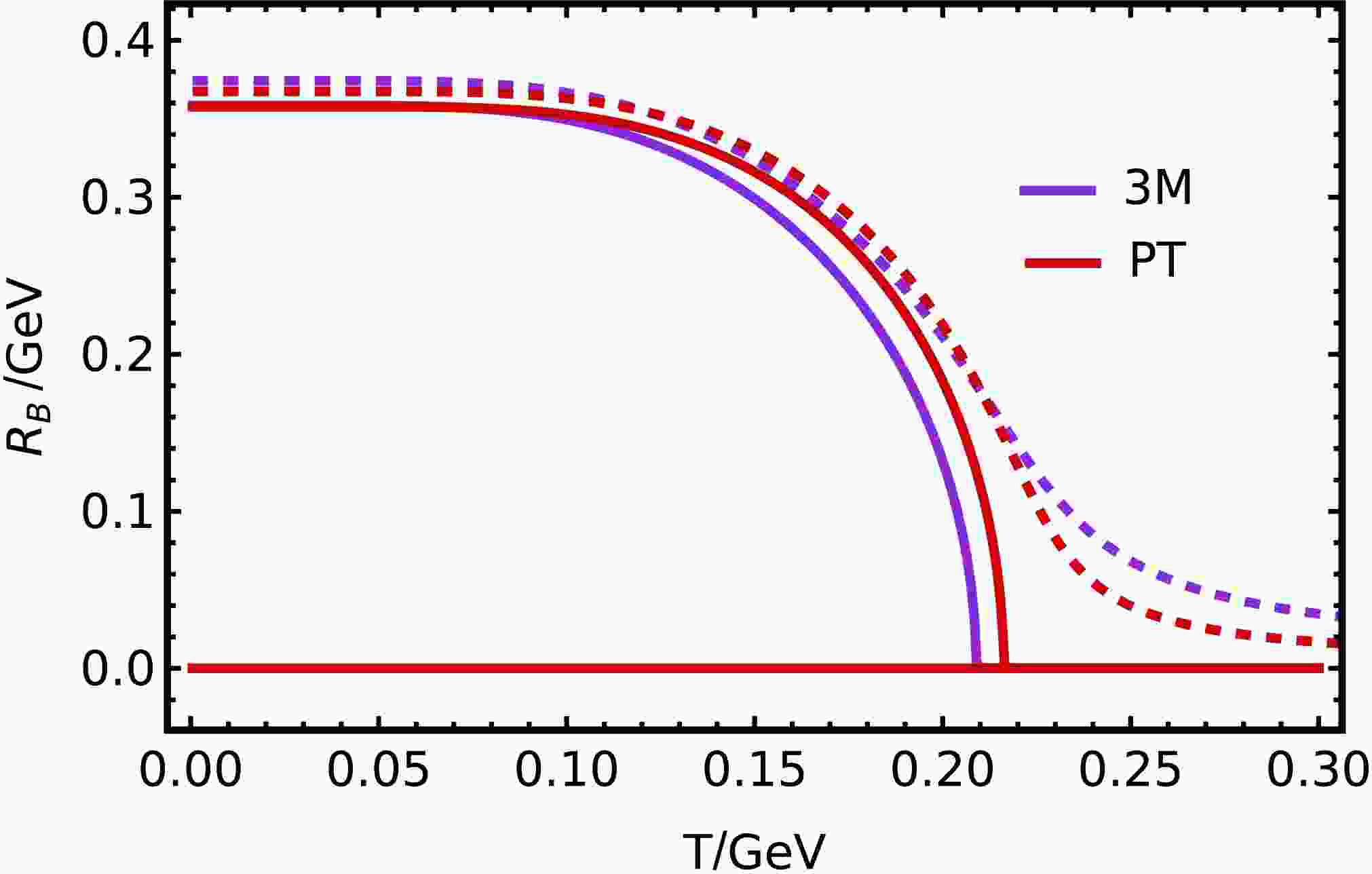
We can see clearly from Fig. 1 that, in the chiral limit ($ m=0 $), the gap equation always has a solution with restored chiral symmetry, i.e. $ R_B=0 $, which is usually referred to as the Wigner solution; see, e.g., [20, 24, 74]. Another solution is the chiral-symmetry-broken Nambu solution, i.e. $ R_B\neq 0 $. In the domains where the Nambu and Wigner solutions coexist, the thermodynamically stable branch is the one that minimizes the thermodynamic potential. At low temperature, this is the Nambu solution. As the temperature increases, the system undergoes a second-order phase transition to the Wigner phase. [24, 34, 36] However, beyond the chiral limit, only the Nambu solution exists, and the transition becomes a crossover, as has been widely discussed in the literature [36, 75–78]. Moreover, it is interesting to note that the 3M and PT regularization schemes yield very similar results, both qualitatively and quantitatively.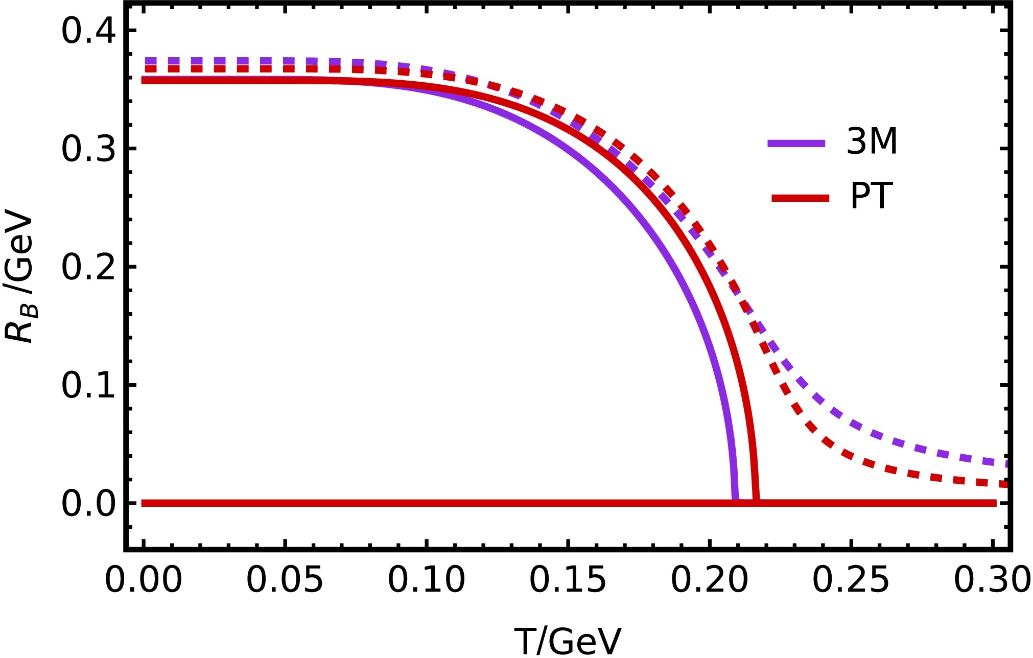

Figure 1.  (color online) Gap-equation solutions at $ \mu=0 $ obtained with the PT and 3M regularization schemes. Here, CL (solid) corresponds to the chiral limit ($ m=0 $), and BC (dashed) corresponds to $ m=0.007 $ GeV.

The normalized pressure $ P/P_{\rm SB} $ as a function of T is presented in Fig. 2 for different regularization schemes, where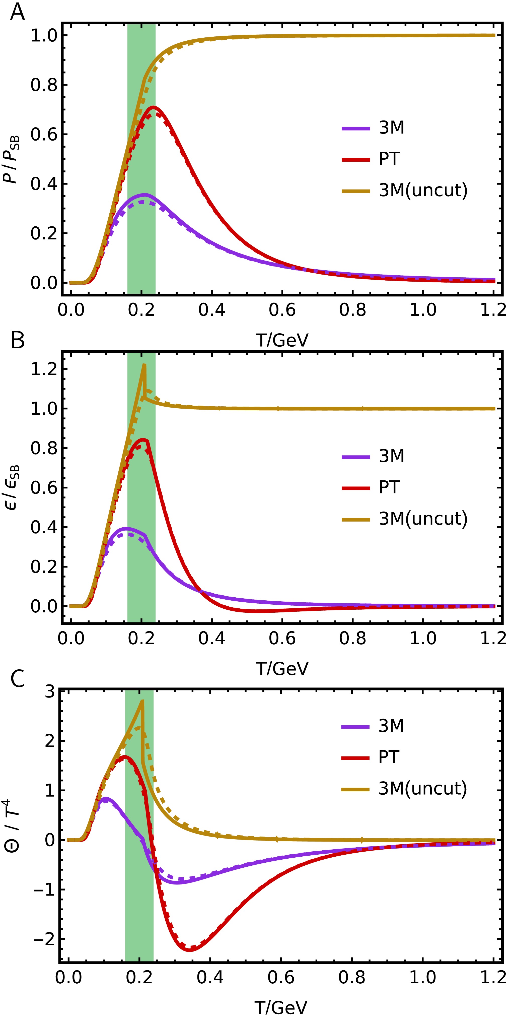

Figure 2.  (color online) The temperature dependence of the normalized pressure $P/P_{\rm SB}$, energy density $\epsilon/\epsilon_{\rm SB}$, and trace anomaly $ \Theta/T^4 $ is shown for the 3M cutoff, PT regularization, and uncut cases. The solid and dashed lines correspond to the CL and BC cases, respectively. The green shaded region, $ T\in[0.16,0.24] $ GeV, denotes the transition region of interest.

denotes the Stefan–Boltzmann (SB) pressure of an ideal massless fermion gas [72].

It can be seen from Fig. 2A that the uncut scheme gradually approaches the correct SB limit with increasing temperature. This indicates that the high-T behavior can be smoothly connected to the perturbative QCD (pQCD) limit. In contrast, the full 3M scheme suppresses not only the vacuum contribution but also thermal modes with momenta above the cutoff. Consequently, $P/P_{\rm SB}$ reaches a maximum value of approximately $ 0.355 $ at $ T=210.5 $ MeV and then decreases toward zero at high T, indicating that this scheme fails to recover the SB limit.

Compared with the 3M cutoff scheme, PT regularization exhibits a qualitatively different behavior. Although the PT scheme also does not recover the SB limit because of the suppression of ultraviolet modes, it preserves the dominant thermal contribution in the temperature region around the chiral transition, $ T\approx 215 $ MeV, which is the main focus of this work. Therefore, the PT-regularized result maintains a closer connection to the high-T pQCD behavior in the physically relevant crossover region.

Similarly, as shown by the energy density and trace anomaly in Fig. 2B and Fig. 2C, respectively, the results obtained with the uncut scheme approach the SB limit

at high T. Compared with the 3M regularization scheme, PT regularization also retains a larger fraction of the thermal contributions in the transition region of interest and consequently exhibits better agreement with the expected pQCD behavior in the crossover region.

Nevertheless, the PT-regularized energy density becomes slightly negative for $ T>0.4 $ GeV. This occurs because, in the high-T limit, the pressure in the PT scheme approaches a small positive constant rather than vanishing. Such behavior is not a physically reasonable prediction of QCD and should instead be regarded as an unphysical artifact introduced by applying PT regularization to the thermal contributions.

The above observations can be seen more directly from the trace anomaly shown in Fig. 2C. At relatively low T, $ \nu_T $ increases rapidly with T, signaling the activation of quark thermal degrees of freedom and a pronounced departure of the system from conformal behavior. The positive peak obtained with PT regularization is substantially higher than that produced by the 3M scheme and lies closer to the result obtained without regularizing the thermal contribution. This confirms that PT regularization preserves a larger fraction of the dominant thermal effects around the chiral transition, whereas the fixed three-momentum cutoff significantly suppresses the liberation of thermal degrees of freedom.

Beyond the peak, the trace anomaly decreases rapidly. The result without a thermal cutoff remains positive over the entire temperature range, indicating that $ \nu_T $ increases monotonically and approaches the SB limit from below. By contrast, the 3M and PT results cross zero, with each zero crossing corresponding to a maximum of $ \nu_T $. At higher temperatures, $ \Theta/T^4 $ becomes negative, implying that $ \nu_T $ decreases. This behavior shows that these regularization schemes fail to retain the complete thermal phase space required at increasing T, so that regularization effects progressively dominate the thermodynamic behavior.

The negative minimum in the 3M result is relatively shallow but appears at a lower T, indicating earlier suppression of thermal modes by the fixed momentum cutoff. In contrast, PT develops a deeper and broader negative minimum at higher T. Therefore, PT provides a better description of the crossover region, although its regularization artifacts become more pronounced in the high-T regime.

We can see clearly from Fig. 1 that, in the chiral limit ($ m=0 $), the gap equation always has a solution with restored chiral symmetry, i.e. $ R_B=0 $, which is usually referred to as the Wigner solution; see, e.g., [20, 24, 74]. Another solution is the chiral-symmetry-broken Nambu solution, i.e. $ R_B\neq 0 $. In the domains where the Nambu and Wigner solutions coexist, the thermodynamically stable branch is the one that minimizes the thermodynamic potential. At low temperature, this is the Nambu solution. As the temperature increases, the system undergoes a second-order phase transition to the Wigner phase. [24, 34, 36] However, beyond the chiral limit, only the Nambu solution exists, and the transition becomes a crossover, as has been widely discussed in the literature [36, 75–78]. Moreover, it is interesting to note that the 3M and PT regularization schemes yield very similar results, both qualitatively and quantitatively.

Figure 1.  (color online) Gap-equation solutions at $ \mu=0 $ obtained with the PT and 3M regularization schemes. Here, CL (solid) corresponds to the chiral limit ($ m=0 $), and BC (dashed) corresponds to $ m=0.007 $ GeV.

The normalized pressure $ P/P_{\rm SB} $ as a function of T is presented in Fig. 2 for different regularization schemes, where

Figure 2.  (color online) The temperature dependence of the normalized pressure $P/P_{\rm SB}$, energy density $\epsilon/\epsilon_{\rm SB}$, and trace anomaly $ \Theta/T^4 $ is shown for the 3M cutoff, PT regularization, and uncut cases. The solid and dashed lines correspond to the CL and BC cases, respectively. The green shaded region, $ T\in[0.16,0.24] $ GeV, denotes the transition region of interest.

denotes the Stefan–Boltzmann (SB) pressure of an ideal massless fermion gas [72].

It can be seen from Fig. 2A that the uncut scheme gradually approaches the correct SB limit with increasing temperature. This indicates that the high-T behavior can be smoothly connected to the perturbative QCD (pQCD) limit. In contrast, the full 3M scheme suppresses not only the vacuum contribution but also thermal modes with momenta above the cutoff. Consequently, $P/P_{\rm SB}$ reaches a maximum value of approximately $ 0.355 $ at $ T=210.5 $ MeV and then decreases toward zero at high T, indicating that this scheme fails to recover the SB limit.

Compared with the 3M cutoff scheme, PT regularization exhibits a qualitatively different behavior. Although the PT scheme also does not recover the SB limit because of the suppression of ultraviolet modes, it preserves the dominant thermal contribution in the temperature region around the chiral transition, $ T\approx 215 $ MeV, which is the main focus of this work. Therefore, the PT-regularized result maintains a closer connection to the high-T pQCD behavior in the physically relevant crossover region.

Similarly, as shown by the energy density and trace anomaly in Fig. 2B and Fig. 2C, respectively, the results obtained with the uncut scheme approach the SB limit

at high T. Compared with the 3M regularization scheme, PT regularization also retains a larger fraction of the thermal contributions in the transition region of interest and consequently exhibits better agreement with the expected pQCD behavior in the crossover region.

Nevertheless, the PT-regularized energy density becomes slightly negative for $ T>0.4 $ GeV. This occurs because, in the high-T limit, the pressure in the PT scheme approaches a small positive constant rather than vanishing. Such behavior is not a physically reasonable prediction of QCD and should instead be regarded as an unphysical artifact introduced by applying PT regularization to the thermal contributions.

The above observations can be seen more directly from the trace anomaly shown in Fig. 2C. At relatively low T, $ \nu_T $ increases rapidly with T, signaling the activation of quark thermal degrees of freedom and a pronounced departure of the system from conformal behavior. The positive peak obtained with PT regularization is substantially higher than that produced by the 3M scheme and lies closer to the result obtained without regularizing the thermal contribution. This confirms that PT regularization preserves a larger fraction of the dominant thermal effects around the chiral transition, whereas the fixed three-momentum cutoff significantly suppresses the liberation of thermal degrees of freedom.

Beyond the peak, the trace anomaly decreases rapidly. The result without a thermal cutoff remains positive over the entire temperature range, indicating that $ \nu_T $ increases monotonically and approaches the SB limit from below. By contrast, the 3M and PT results cross zero, with each zero crossing corresponding to a maximum of $ \nu_T $. At higher temperatures, $ \Theta/T^4 $ becomes negative, implying that $ \nu_T $ decreases. This behavior shows that these regularization schemes fail to retain the complete thermal phase space required at increasing T, so that regularization effects progressively dominate the thermodynamic behavior.

The negative minimum in the 3M result is relatively shallow but appears at a lower T, indicating earlier suppression of thermal modes by the fixed momentum cutoff. In contrast, PT develops a deeper and broader negative minimum at higher T. Therefore, PT provides a better description of the crossover region, although its regularization artifacts become more pronounced in the high-T regime.

We consider the $ T\to 0 $ case, as shown in Fig. 3. In the 3M regularization, as shown in Fig. 3A, we clearly observe a first-order phase transition. Beyond the chiral limit, the Nambu and Wigner solutions coexist in the region $ \mu\approx 398.5 $–$ 400 $ MeV. For the PT regularization scheme, the picture changes significantly. As shown in Fig. 3B, the pattern is almost the same as that in Fig. 1, except that $ R_C $ becomes nonzero and increases gradually with μ. Namely, in this scheme, the effect of μ is very similar to that of T. From Fig. 3, we also note that $ R_C=0 $ is a good approximation at low μ, whereas at large μ, the effect of $ R_C $ becomes non-negligible.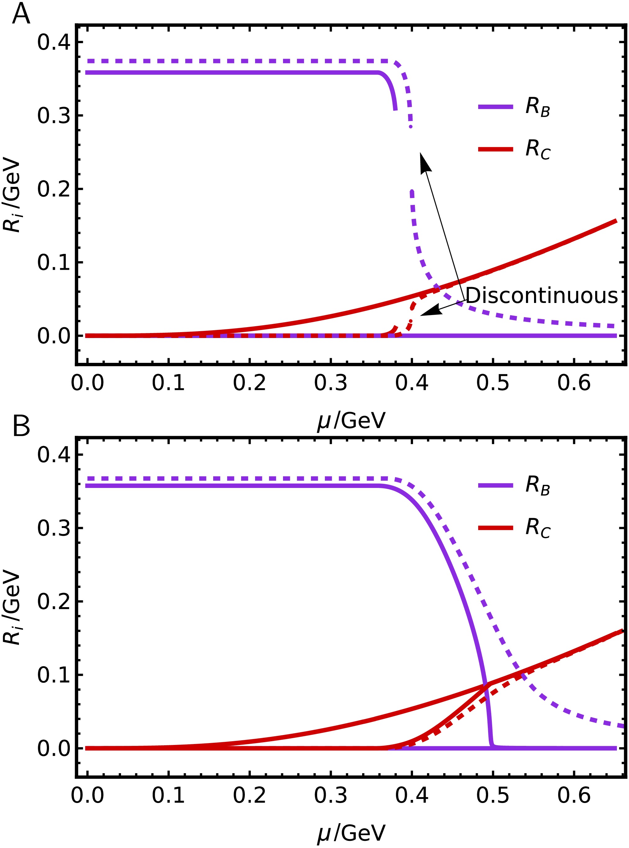

Figure 3.  (color online) Solutions of the gap equation with different regularization schemes in the limit $ T \to 0 $. Panel A: 3M regularization; Panel B: PT regularization. The solid and dashed lines correspond to the CL and BC cases, respectively.

Comparing Fig. 1 and Fig. 3, we find that, within the present SCI and for the parameter sets considered, the qualitative effect of increasing T at zero μ is similar in both schemes, whereas with increasing μ at low T, the two regularization prescriptions yield different transition patterns.

The normalized pressure $P/P_{\rm FD}$, energy density $\epsilon/\epsilon_{\rm FD}$, sound velocity $ c_s^2 $, and trace anomaly $ \Theta/\mu^4 $ as functions of μ are shown in Fig. 4, where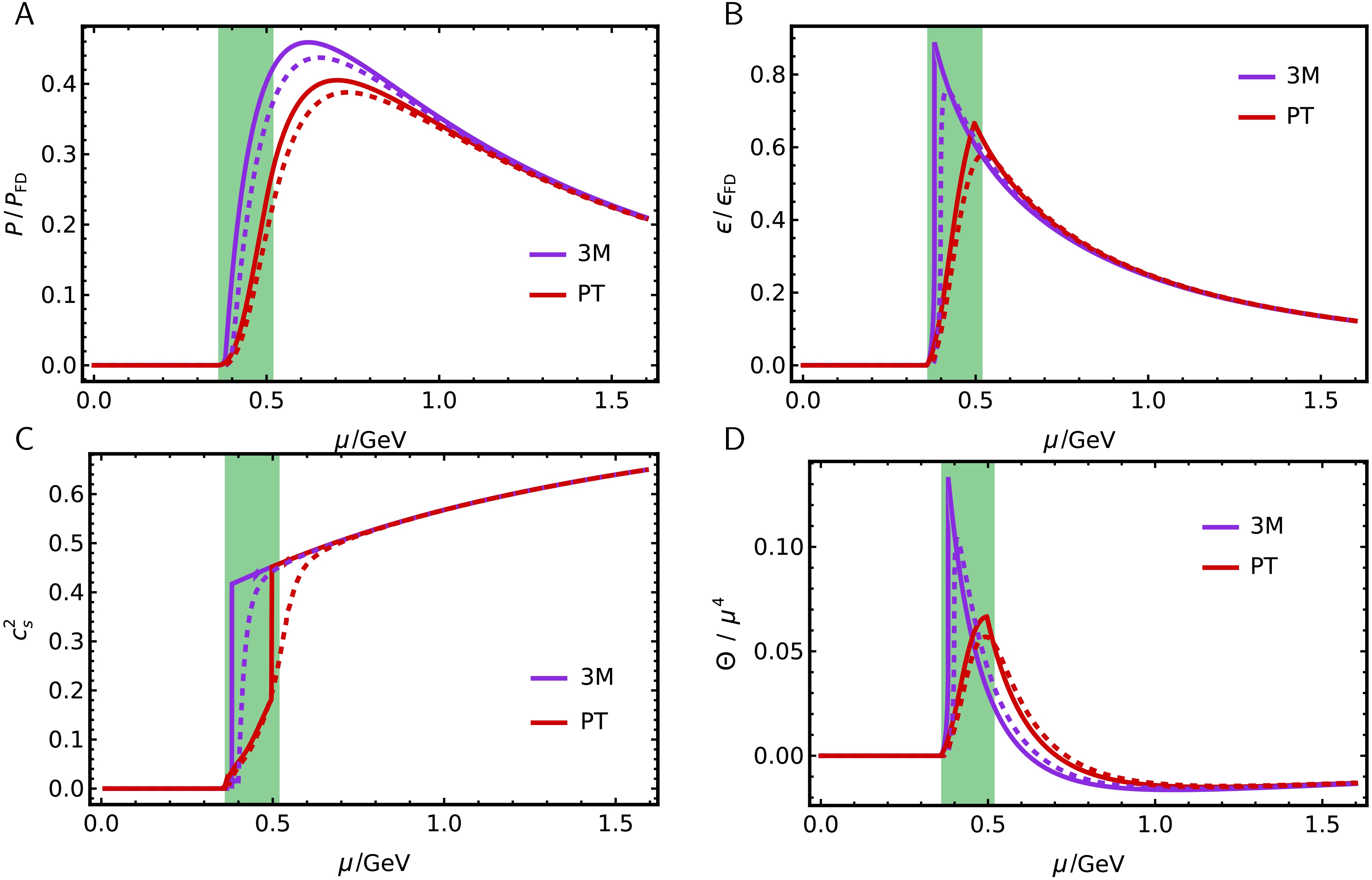

Figure 4.  (color online) The μ dependence of the normalized pressure $P/P_{\rm FD}$, energy density $\epsilon/\epsilon_{\rm FD}$, sound velocity $ c_s^2 $, and trace anomaly $ \Theta/\mu^4 $ in the 3M cutoff and PT regularization schemes. The solid and dashed lines correspond to the CL and BC cases, respectively. The green shaded region, $ \mu\in[0.36, 0.52] $ GeV, denotes the transition region of interest.

As can be seen from the four figures, neither the 3M nor the PT scheme approaches the FD limit in the high-μ regime. This is because no regularization is applied to $ R_C $ in Eq. (42). Consequently, at large chemical potential, the system's behavior is dominated by the vector repulsive interaction.

In contrast, because $ R_B $ approaches zero at high μ, the dependence on the regularization scheme becomes negligible, leading to nearly identical results for the 3M and PT schemes when $ \mu>0.7 $ GeV. Therefore, the high-μ behavior is governed primarily by the vector repulsive interaction, which yields an excessively stiff equation of state and prevents the recovery of the free-quark-gas or perturbative-QCD limits. This behavior reflects a limitation of the contact interaction rather than a property of asymptotically dense QCD matter. Introducing μ-dependent couplings or employing more sophisticated momentum-dependent interaction kernels may improve the high-μ behavior.

Meanwhile, in the transition region of interest, $ \mu\in[0.36,0.52] $ GeV, the first-order transition obtained with the 3M scheme induces abrupt changes in $ R_B $ and $ R_C $ around the phase boundary. As a result, the normalized pressure in the 3M scheme exhibits a steeper slope and a larger peak than that in the PT scheme, although this peak remains below the FD limit. Similar behavior is observed for the energy density. Hence, the regularization dependence manifests itself mainly through the different phase-transition structures, whereas the thermodynamic behavior away from the transition region is almost insensitive to the choice of regularization scheme.

For the squared speed of sound shown in Fig. 4C, we find that, for finite current quark mass, the results obtained with the 3M and PT schemes exceed the conformal value $ c_s^2=1/3 $ at $ \mu\simeq0.428 $ GeV and $ \mu\simeq0.537 $ GeV, respectively. Subsequently, the two results gradually merge and approach the causal limit $ c_s^2=1 $. This behavior is also inconsistent with the expected asymptotic behavior of pQCD, in which the equation of state should approach the conformal limit with $ c_s^2\rightarrow 1/3 $. Instead, it indicates an excessively stiff equation of state induced by the persistent vector repulsive interaction at high density.

For the trace anomaly shown in Fig. 4D, the 3M scheme exhibits a larger peak than the PT scheme in the transition region, indicating stronger breaking of conformal symmetry and a more rapid change in the thermodynamic degrees of freedom across the phase transition. Similar to the T-dependent case, the trace anomaly subsequently decreases, crosses zero, becomes negative, and finally approaches zero at large chemical potential.

We consider the $ T\to 0 $ case, as shown in Fig. 3. In the 3M regularization, as shown in Fig. 3A, we clearly observe a first-order phase transition. Beyond the chiral limit, the Nambu and Wigner solutions coexist in the region $ \mu\approx 398.5 $–$ 400 $ MeV. For the PT regularization scheme, the picture changes significantly. As shown in Fig. 3B, the pattern is almost the same as that in Fig. 1, except that $ R_C $ becomes nonzero and increases gradually with μ. Namely, in this scheme, the effect of μ is very similar to that of T. From Fig. 3, we also note that $ R_C=0 $ is a good approximation at low μ, whereas at large μ, the effect of $ R_C $ becomes non-negligible.

Figure 3.  (color online) Solutions of the gap equation with different regularization schemes in the limit $ T \to 0 $. Panel A: 3M regularization; Panel B: PT regularization. The solid and dashed lines correspond to the CL and BC cases, respectively.

Comparing Fig. 1 and Fig. 3, we find that, within the present SCI and for the parameter sets considered, the qualitative effect of increasing T at zero μ is similar in both schemes, whereas with increasing μ at low T, the two regularization prescriptions yield different transition patterns.

The normalized pressure $P/P_{\rm FD}$, energy density $\epsilon/\epsilon_{\rm FD}$, sound velocity $ c_s^2 $, and trace anomaly $ \Theta/\mu^4 $ as functions of μ are shown in Fig. 4, where

Figure 4.  (color online) The μ dependence of the normalized pressure $P/P_{\rm FD}$, energy density $\epsilon/\epsilon_{\rm FD}$, sound velocity $ c_s^2 $, and trace anomaly $ \Theta/\mu^4 $ in the 3M cutoff and PT regularization schemes. The solid and dashed lines correspond to the CL and BC cases, respectively. The green shaded region, $ \mu\in[0.36, 0.52] $ GeV, denotes the transition region of interest.

As can be seen from the four figures, neither the 3M nor the PT scheme approaches the FD limit in the high-μ regime. This is because no regularization is applied to $ R_C $ in Eq. (42). Consequently, at large chemical potential, the system's behavior is dominated by the vector repulsive interaction.

In contrast, because $ R_B $ approaches zero at high μ, the dependence on the regularization scheme becomes negligible, leading to nearly identical results for the 3M and PT schemes when $ \mu>0.7 $ GeV. Therefore, the high-μ behavior is governed primarily by the vector repulsive interaction, which yields an excessively stiff equation of state and prevents the recovery of the free-quark-gas or perturbative-QCD limits. This behavior reflects a limitation of the contact interaction rather than a property of asymptotically dense QCD matter. Introducing μ-dependent couplings or employing more sophisticated momentum-dependent interaction kernels may improve the high-μ behavior.

Meanwhile, in the transition region of interest, $ \mu\in[0.36,0.52] $ GeV, the first-order transition obtained with the 3M scheme induces abrupt changes in $ R_B $ and $ R_C $ around the phase boundary. As a result, the normalized pressure in the 3M scheme exhibits a steeper slope and a larger peak than that in the PT scheme, although this peak remains below the FD limit. Similar behavior is observed for the energy density. Hence, the regularization dependence manifests itself mainly through the different phase-transition structures, whereas the thermodynamic behavior away from the transition region is almost insensitive to the choice of regularization scheme.

For the squared speed of sound shown in Fig. 4C, we find that, for finite current quark mass, the results obtained with the 3M and PT schemes exceed the conformal value $ c_s^2=1/3 $ at $ \mu\simeq0.428 $ GeV and $ \mu\simeq0.537 $ GeV, respectively. Subsequently, the two results gradually merge and approach the causal limit $ c_s^2=1 $. This behavior is also inconsistent with the expected asymptotic behavior of pQCD, in which the equation of state should approach the conformal limit with $ c_s^2\rightarrow 1/3 $. Instead, it indicates an excessively stiff equation of state induced by the persistent vector repulsive interaction at high density.

For the trace anomaly shown in Fig. 4D, the 3M scheme exhibits a larger peak than the PT scheme in the transition region, indicating stronger breaking of conformal symmetry and a more rapid change in the thermodynamic degrees of freedom across the phase transition. Similar to the T-dependent case, the trace anomaly subsequently decreases, crosses zero, becomes negative, and finally approaches zero at large chemical potential.

To clearly demonstrate the influence of the vector mean field $ R_C $, we employ 3M regularization and set $ \Lambda_{3M}=0.58 $ GeV. As shown in Fig. 5, this changes the first-order phase transition previously observed in Fig. 3A into a crossover. If we set $ R_C=0 $, the curve shifts to lower μ and becomes first-order again. Evidently, this indicates that $ R_C $ has a significant effect on the order of the phase transition and weakens the first-order phase transition.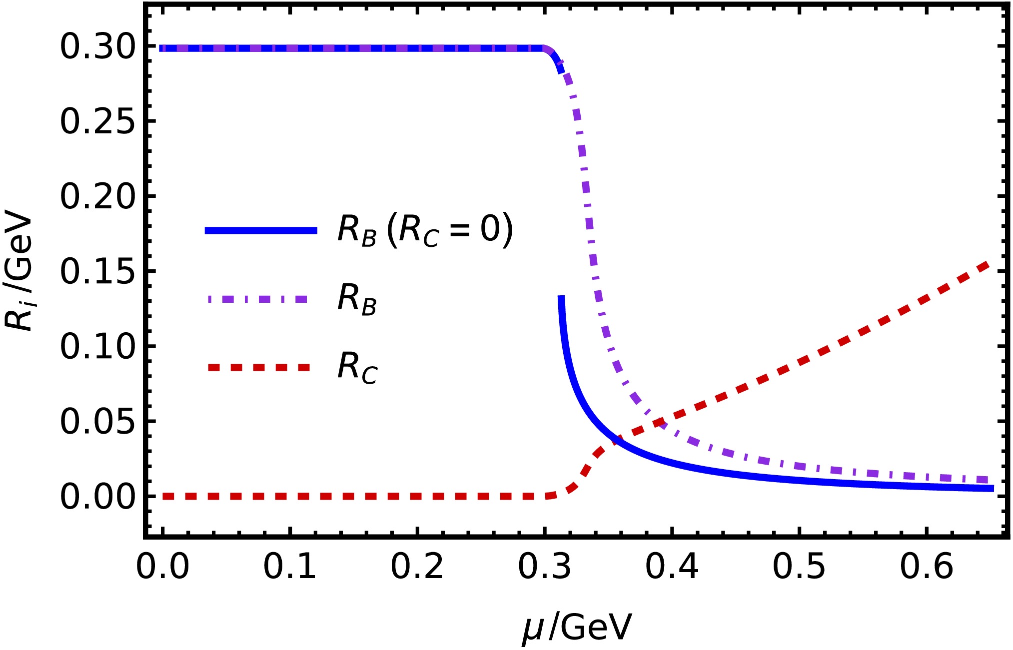

Figure 5.  (color online) $ R_C $ effect on the phase transition in the 3M regularization scheme. All other parameters are taken from Table 1, except that $ \Lambda_{3M}=0.58 $ GeV. The solid blue curve shows $ R_B $ obtained with $ R_C=0 $; the dot-dashed purple and dashed red curves show the self-consistent $ R_B $ and $ R_C $, respectively.

The key point originates from the minus sign in the effective chemical potential, $ \mu'=\mu-R_C $, which reflects the repulsive nature of the vector interaction among quarks [14, 79, 80]. Since $ R_C\propto \langle \psi^\dagger \psi\rangle $ increases with the quark number density, the repulsion becomes stronger as the system becomes denser. Consequently, achieving a further increase in density requires a larger external chemical potential to compensate for this enhanced internal repulsion. In other words, $ R_C $ systematically suppresses the effect of the chemical potential on the thermodynamic potential. This mechanism naturally leads to a weakening of the first-order chiral phase transition at high density.

Next, we analyze how the regularization schemes alter the order of the phase transition. As mentioned above, because the SCI framework is nonrenormalizable, one must introduce a special treatment to cure the ultraviolet divergence and render the quantities finite. Comparing Eq. (44) and Eq. (45), we find that the 3M regularization scheme imposes a hard cutoff, $ \Lambda_{3M}^2 $, which eliminates contributions from higher momenta. By contrast, in the PT regularization, the momentum integration extends to $ +\infty $, with a soft cutoff provided by the exponential damping factor $ {\rm e}^{-\tau_{uv}^2\mathcal{T}} $.

To interpolate between the hard cutoff and the soft exponential damping factor, we introduce the following equation

The exponential factor associated with $ \tau_{ir} $ is approximately zero; we neglect it in the present discussion. Using the PT parametrization from Table 1, we vary $ \Lambda_{uv} $ as shown in Table 2. To keep the vacuum mass constant for all $ \Lambda_{uv} $ values, we adjust $ \Lambda_{H} $ accordingly. More specifically, because $ \Lambda_H $ is the only newly introduced parameter in Eq. (51), it is uniquely fixed by requiring $ R_B(T=0, \mu=0)=0.37 $ GeV beyond the chiral limit. In this way, we interpolate from a PT-type solution (A) to a 3M-type solution (F). Fig. 6A shows that, at $ T=0 $, the PT crossover in $ R_B(\mu) $ gradually changes into a first-order phase transition.

Figure 6.  (color online) Comparison of solutions for different parameter sets. Panel A: using six different parameters listed in the upper panel of Table 2. Panel B: using four different parameters listed in the lower panel of Table 2.

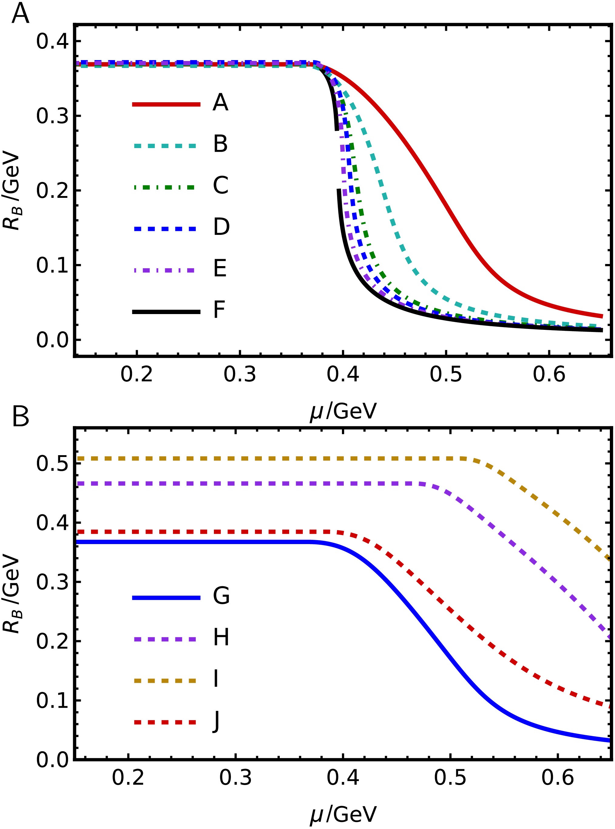
In the present model and parameter interpolation, we find that the 3M cutoff treatment introduces a hard, sharp cutoff in momentum space, which tends to produce more abrupt changes in the behavior of physical quantities. Using the effective mass as an example, we observe a similar pattern in related quantities, manifested as a first-order phase transition. By contrast, the PT regularization smoothly suppresses the interaction through an exponential damping factor. Because this suppression is gradual, most related quantities and processes also tend to change continuously, manifested as a crossover.

Finally, we discuss the influence of the remaining parameters on the phase transition. To assess the parameter sensitivity of the PT result, we performed a numerical scan over $ \Lambda_{\rm uv}\in[0.8,1.1] $ GeV, $ \alpha_{ir}\in[0.8\pi,1.2\pi] $, and $ m\in[0.0001,0.07] $ GeV, while keeping the remaining parameters fixed at their baseline values. Within the sampled parameter grid and numerical resolution, we found no discontinuity or thermodynamic coexistence indicative of a first-order transition under the baseline PT prescription. Thus, all parameter sets explicitly examined here exhibit crossover behavior as $ T\to 0 $. Representative results for several selected parameter sets are shown in Fig. 6B. For the 3M regularization, the transition order is found to be strongly correlated with the dimensionless quantity

This makes it a useful numerical classifier. Figure 7 shows that smaller values of $ \chi\lesssim1.64 $ lead to a crossover at $ m=0.007 $ GeV, whereas $ \chi\gtrsim1.64 $ yields a first-order transition. Although one may set $ R_C=0 $, doing so merely shifts the critical value of χ downward without altering this qualitative behavior.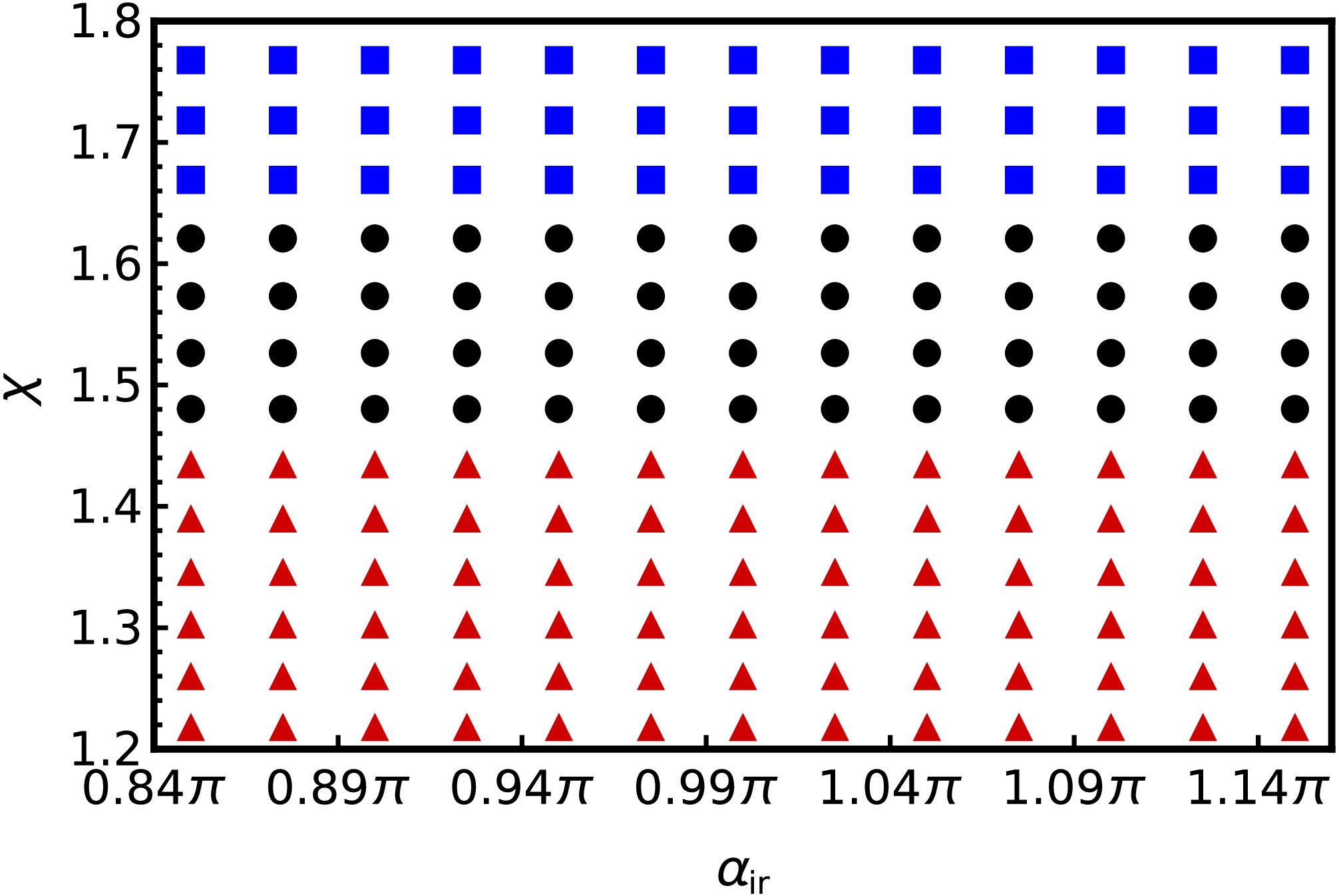

Figure 7.  (color online) Within the parameter sets examined at $ m=0.007 $ GeV, χ is strongly correlated with the order of the transition and serves as an effective numerical classifier. Legend: blue squares—first order for both $ R_C=0 $ and $ R_C\neq0 $; black circles—first order only at $ R_C=0 $ and crossover at $ R_C\neq0 $; red triangles—crossover in both cases.

To clearly demonstrate the influence of the vector mean field $ R_C $, we employ 3M regularization and set $ \Lambda_{3M}=0.58 $ GeV. As shown in Fig. 5, this changes the first-order phase transition previously observed in Fig. 3A into a crossover. If we set $ R_C=0 $, the curve shifts to lower μ and becomes first-order again. Evidently, this indicates that $ R_C $ has a significant effect on the order of the phase transition and weakens the first-order phase transition.

Figure 5.  (color online) $ R_C $ effect on the phase transition in the 3M regularization scheme. All other parameters are taken from Table 1, except that $ \Lambda_{3M}=0.58 $ GeV. The solid blue curve shows $ R_B $ obtained with $ R_C=0 $; the dot-dashed purple and dashed red curves show the self-consistent $ R_B $ and $ R_C $, respectively.

The key point originates from the minus sign in the effective chemical potential, $ \mu'=\mu-R_C $, which reflects the repulsive nature of the vector interaction among quarks [14, 79, 80]. Since $ R_C\propto \langle \psi^\dagger \psi\rangle $ increases with the quark number density, the repulsion becomes stronger as the system becomes denser. Consequently, achieving a further increase in density requires a larger external chemical potential to compensate for this enhanced internal repulsion. In other words, $ R_C $ systematically suppresses the effect of the chemical potential on the thermodynamic potential. This mechanism naturally leads to a weakening of the first-order chiral phase transition at high density.

Next, we analyze how the regularization schemes alter the order of the phase transition. As mentioned above, because the SCI framework is nonrenormalizable, one must introduce a special treatment to cure the ultraviolet divergence and render the quantities finite. Comparing Eq. (44) and Eq. (45), we find that the 3M regularization scheme imposes a hard cutoff, $ \Lambda_{3M}^2 $, which eliminates contributions from higher momenta. By contrast, in the PT regularization, the momentum integration extends to $ +\infty $, with a soft cutoff provided by the exponential damping factor $ {\rm e}^{-\tau_{uv}^2\mathcal{T}} $.

To interpolate between the hard cutoff and the soft exponential damping factor, we introduce the following equation

The exponential factor associated with $ \tau_{ir} $ is approximately zero; we neglect it in the present discussion. Using the PT parametrization from Table 1, we vary $ \Lambda_{uv} $ as shown in Table 2. To keep the vacuum mass constant for all $ \Lambda_{uv} $ values, we adjust $ \Lambda_{H} $ accordingly. More specifically, because $ \Lambda_H $ is the only newly introduced parameter in Eq. (51), it is uniquely fixed by requiring $ R_B(T=0, \mu=0)=0.37 $ GeV beyond the chiral limit. In this way, we interpolate from a PT-type solution (A) to a 3M-type solution (F). Fig. 6A shows that, at $ T=0 $, the PT crossover in $ R_B(\mu) $ gradually changes into a first-order phase transition.

Figure 6.  (color online) Comparison of solutions for different parameter sets. Panel A: using six different parameters listed in the upper panel of Table 2. Panel B: using four different parameters listed in the lower panel of Table 2.

In the present model and parameter interpolation, we find that the 3M cutoff treatment introduces a hard, sharp cutoff in momentum space, which tends to produce more abrupt changes in the behavior of physical quantities. Using the effective mass as an example, we observe a similar pattern in related quantities, manifested as a first-order phase transition. By contrast, the PT regularization smoothly suppresses the interaction through an exponential damping factor. Because this suppression is gradual, most related quantities and processes also tend to change continuously, manifested as a crossover.

Finally, we discuss the influence of the remaining parameters on the phase transition. To assess the parameter sensitivity of the PT result, we performed a numerical scan over $ \Lambda_{\rm uv}\in[0.8,1.1] $ GeV, $ \alpha_{ir}\in[0.8\pi,1.2\pi] $, and $ m\in[0.0001,0.07] $ GeV, while keeping the remaining parameters fixed at their baseline values. Within the sampled parameter grid and numerical resolution, we found no discontinuity or thermodynamic coexistence indicative of a first-order transition under the baseline PT prescription. Thus, all parameter sets explicitly examined here exhibit crossover behavior as $ T\to 0 $. Representative results for several selected parameter sets are shown in Fig. 6B. For the 3M regularization, the transition order is found to be strongly correlated with the dimensionless quantity

This makes it a useful numerical classifier. Figure 7 shows that smaller values of $ \chi\lesssim1.64 $ lead to a crossover at $ m=0.007 $ GeV, whereas $ \chi\gtrsim1.64 $ yields a first-order transition. Although one may set $ R_C=0 $, doing so merely shifts the critical value of χ downward without altering this qualitative behavior.

Figure 7.  (color online) Within the parameter sets examined at $ m=0.007 $ GeV, χ is strongly correlated with the order of the transition and serves as an effective numerical classifier. Legend: blue squares—first order for both $ R_C=0 $ and $ R_C\neq0 $; black circles—first order only at $ R_C=0 $ and crossover at $ R_C\neq0 $; red triangles—crossover in both cases.

We used a contact interaction to compare the effects of different regularization schemes, namely the three-momentum cutoff and proper-time treatments, at nonzero temperature T or chemical potential μ. At $ \mu=0 $ and nonzero T, both regularization schemes yield a second-order phase transition in the chiral limit and a smooth crossover for a finite current quark mass. In the low-T, nonzero-μ region, however, different regularization schemes and parametrizations may produce qualitatively distinct behavior, namely either a crossover or a first-order transition. Within the nonrenormalizable SCI model and the parameter ranges explored in this work, we find no evidence of a first-order transition for the tested proper-time prescriptions, although their quantitative predictions differ. In contrast, the three-momentum cutoff scheme can produce either crossover-like or first-order behavior, depending on the chosen parameters.

This sensitivity is problematic. In a renormalizable quantum field theory, the phase structure is expected to be independent of the regularization procedure, provided that it is implemented consistently. In this study, we matched the vacuum dynamical mass and the corresponding condensate while keeping the underlying interaction parameters fixed. In conclusion, for the nonrenormalizable contact model, the regulator is effectively part of the model definition, and predictions concerning the phase structure in medium are intrinsically scheme dependent.

The thermodynamic analysis shows that the prescription retaining the full thermal contribution recovers the Stefan–Boltzmann limit at asymptotically high temperature, consistent with the expected high-temperature behavior of QCD. Around the thermal crossover at $ \mu=0 $, proper-time regularization retains more relevant thermal contributions than the three-momentum cutoff. At zero T and nonzero μ, the first-order transition produced by the three-momentum cutoff generates sharper structures in the pressure, energy density, and trace anomaly than the smooth proper-time result. In the high-μ region, the two schemes exhibit a common high-density behavior, which is dominated by the persistent vector self-energy $ R_C $, producing an excessively stiff equation of state and preventing recovery of the free-gas or pQCD limit. These results distinguish regularization effects near the transition from the intrinsic high-energy limitations of the SCI model.

We further compared the NJL mean-field equations with the DS equations for a contact interaction and found an approximate equivalence at fixed $ N_c $ after parameter matching. This equivalence is functional rather than structural, as the coefficients exhibit different large-$ N_c $ limits.

At the same time, the bare-vertex approximation violates the Ward identity at nonzero chemical potential, indicating that adopting a symmetry-consistent vertex, such as the Ball–Chiu vertex, is a natural step for future refinement.

We used a contact interaction to compare the effects of different regularization schemes, namely the three-momentum cutoff and proper-time treatments, at nonzero temperature T or chemical potential μ. At $ \mu=0 $ and nonzero T, both regularization schemes yield a second-order phase transition in the chiral limit and a smooth crossover for a finite current quark mass. In the low-T, nonzero-μ region, however, different regularization schemes and parametrizations may produce qualitatively distinct behavior, namely either a crossover or a first-order transition. Within the nonrenormalizable SCI model and the parameter ranges explored in this work, we find no evidence of a first-order transition for the tested proper-time prescriptions, although their quantitative predictions differ. In contrast, the three-momentum cutoff scheme can produce either crossover-like or first-order behavior, depending on the chosen parameters.

This sensitivity is problematic. In a renormalizable quantum field theory, the phase structure is expected to be independent of the regularization procedure, provided that it is implemented consistently. In this study, we matched the vacuum dynamical mass and the corresponding condensate while keeping the underlying interaction parameters fixed. In conclusion, for the nonrenormalizable contact model, the regulator is effectively part of the model definition, and predictions concerning the phase structure in medium are intrinsically scheme dependent.

The thermodynamic analysis shows that the prescription retaining the full thermal contribution recovers the Stefan–Boltzmann limit at asymptotically high temperature, consistent with the expected high-temperature behavior of QCD. Around the thermal crossover at $ \mu=0 $, proper-time regularization retains more relevant thermal contributions than the three-momentum cutoff. At zero T and nonzero μ, the first-order transition produced by the three-momentum cutoff generates sharper structures in the pressure, energy density, and trace anomaly than the smooth proper-time result. In the high-μ region, the two schemes exhibit a common high-density behavior, which is dominated by the persistent vector self-energy $ R_C $, producing an excessively stiff equation of state and preventing recovery of the free-gas or pQCD limit. These results distinguish regularization effects near the transition from the intrinsic high-energy limitations of the SCI model.

We further compared the NJL mean-field equations with the DS equations for a contact interaction and found an approximate equivalence at fixed $ N_c $ after parameter matching. This equivalence is functional rather than structural, as the coefficients exhibit different large-$ N_c $ limits.

At the same time, the bare-vertex approximation violates the Ward identity at nonzero chemical potential, indicating that adopting a symmetry-consistent vertex, such as the Ball–Chiu vertex, is a natural step for future refinement.

We thank C. D. Roberts for valuable suggestions.

We thank C. D. Roberts for valuable suggestions.

As discussed in Eq. (18), restricting the PT integration to a finite interval causes the regularized kernel to depend explicitly on the auxiliary mapping $ \mathcal T' $.

To determine whether the crossover obtained with our baseline prescription arises specifically from the choice $ \mathcal T'=\text{Sign}(\Re_{\mathcal T})\mathcal T $, we compare the following three representative mappings

These mappings provide exponential damping in the PT kernel. More importantly, all three satisfy $ \mathcal T'_j(\mathcal T)=\mathcal T $ for $ \mathcal T>0 $ and therefore reproduce the same vacuum properties. They differ only once $ \mathcal T $ becomes complex at nonzero chemical potential.

The same vacuum parameters and coupled gap equations are used in all three calculations. The results at $ T=0 $ are shown in Fig. A1. From the figure, we note that none of these representative prescriptions provides evidence of a first-order transition in the solutions examined.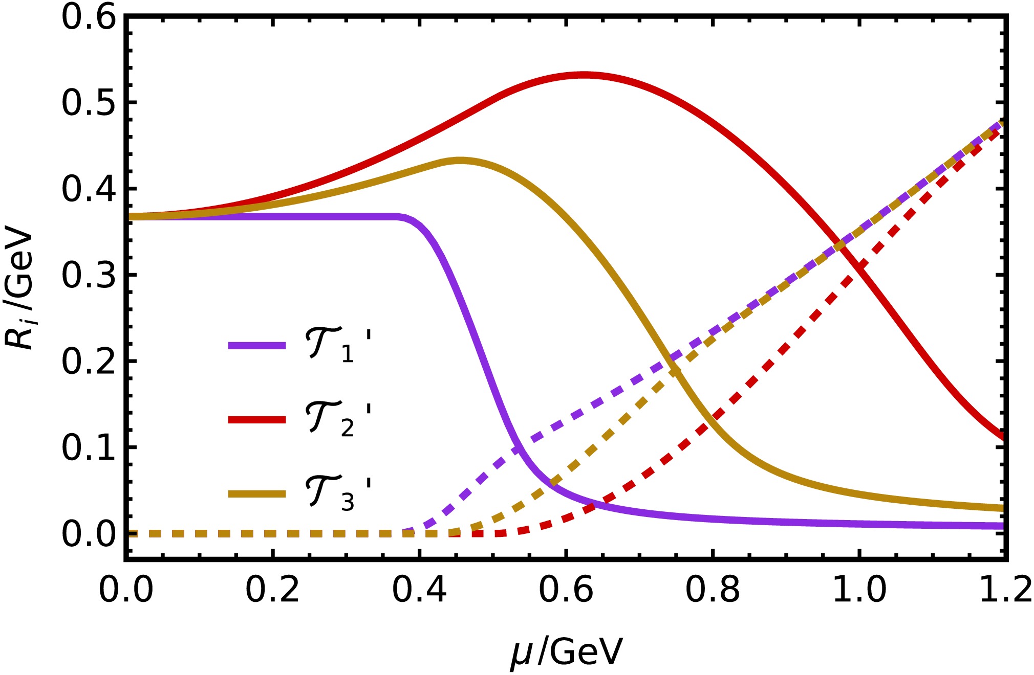

Figure A1.  (color online) Solutions obtained with PT regularization for three representative mappings $ \mathcal T'_j $ beyond the chiral limit in the $ T=0 $ region. The solid and dashed lines correspond to $ R_B $ and $ R_C $, respectively.

The increase in $ R_B $ produced by $ \mathcal T'_2 $ and $ \mathcal T'_3 $ at low chemical potential requires particular caution. Although both mappings reproduce the vacuum kernel exactly at $ \mu=0 $, their nonholomorphic dependence on the complex quantity $ \mathcal T $ introduces an artificial chemical-potential dependence below the critical μ values. We therefore do not regard these curves as quantitatively reliable physical predictions. Their role is solely to test whether substantial deformations of the finite-chemical-potential PT kernel generate a first-order transition.

As discussed in Eq. (18), restricting the PT integration to a finite interval causes the regularized kernel to depend explicitly on the auxiliary mapping $ \mathcal T' $.

To determine whether the crossover obtained with our baseline prescription arises specifically from the choice $ \mathcal T'=\text{Sign}(\Re_{\mathcal T})\mathcal T $, we compare the following three representative mappings

These mappings provide exponential damping in the PT kernel. More importantly, all three satisfy $ \mathcal T'_j(\mathcal T)=\mathcal T $ for $ \mathcal T>0 $ and therefore reproduce the same vacuum properties. They differ only once $ \mathcal T $ becomes complex at nonzero chemical potential.

The same vacuum parameters and coupled gap equations are used in all three calculations. The results at $ T=0 $ are shown in Fig. A1. From the figure, we note that none of these representative prescriptions provides evidence of a first-order transition in the solutions examined.

Figure A1.  (color online) Solutions obtained with PT regularization for three representative mappings $ \mathcal T'_j $ beyond the chiral limit in the $ T=0 $ region. The solid and dashed lines correspond to $ R_B $ and $ R_C $, respectively.

The increase in $ R_B $ produced by $ \mathcal T'_2 $ and $ \mathcal T'_3 $ at low chemical potential requires particular caution. Although both mappings reproduce the vacuum kernel exactly at $ \mu=0 $, their nonholomorphic dependence on the complex quantity $ \mathcal T $ introduces an artificial chemical-potential dependence below the critical μ values. We therefore do not regard these curves as quantitatively reliable physical predictions. Their role is solely to test whether substantial deformations of the finite-chemical-potential PT kernel generate a first-order transition.