Flavor tomography of long-lived neutrino-mass mediators: probing the neutrino mass ordering at the HL-LHC

The neutrino mass ordering—Normal Hierarchy (NH: $ m_3 \gg m_1, m_2 $) or Inverted Hierarchy (IH: $ m_1 \approx m_2 \gg m_3 $)—remains one of the central open questions in particle physics [1–4]. The joint T2K and NOνA analysis [5] finds no strong preference for either mass ordering, and a definitive resolution remains elusive because of persistent $ \delta_{\rm CP} $–hierarchy degeneracies. The oscillation probability $ P(\nu_\mu \to \nu_e) $ in matter is entangled with the unknown CP phase $ \delta_{\rm CP} $, forcing each long-baseline experiment to measure both quantities simultaneously and thereby significantly reducing sensitivity. JUNO [6, 7] has recently begun taking data and aims to determine the ordering via reactor antineutrino vacuum oscillations, independently of $ \delta_{\rm CP} $, within $ {\sim}6.5 $ years; definitive confirmation from long-baseline experiments will require DUNE [8] and Hyper-K [9] on a decadal timescale.

The HL-LHC precision timing detectors—the MIP Timing Detector (MTD) at CMS [10] and the High-Granularity Timing Detector (HGTD) at ATLAS [11]—provide a structurally different probe. With $ {\sim}30\; {\rm{ps}} $ time resolution, they isolate long-lived particle (LLP) decay products through a time-delay requirement $ \Delta t \gt 200\; {\rm{ps}} $, suppressing prompt Standard Model backgrounds to levels that can be estimated with data-driven timing sidebands [12]. In this Letter, we show that when the LLP is the mediator responsible for Majorana neutrino masses, the flavor ratio $ N_e/ N_\mu $ of time-delayed leptons is a $ \delta_{\rm CP} $-independent hierarchy discriminant fixed entirely by Pontecorvo–Maki–Nakagawa–Sakata (PMNS) mixing angles and neutrino mass eigenvalues—a connection not identified in prior work [13–15]. We refer to this measurement strategy as flavor tomography: the flavor composition of the LLP decay products directly images the underlying neutrino mass spectrum, so counting displaced electrons and muons reconstructs information about the mass ordering.

Using collider lepton-flavor counting to probe the neutrino mass hierarchy has a long history. Earlier work showed that the branching ratios of doubly-charged Higgs bosons in the Type-II seesaw [16, 17], triplet-fermion decays in the Type-III seesaw [18], four-lepton signatures at future colliders [19], and heavy neutral lepton (HNL) decays at Z factories [20] all carry an imprint of the mass ordering. These approaches share three limitations. First, they depend on specific model architectures—Type-II or Type-III seesaw, or two-HNL Type-I—and their discriminating power is not portable to other neutrino mass models. Second, none exploits precision timing: they rely on prompt or mildly displaced signatures and require conventional detector simulation to relate observed event rates to theoretical predictions. Third, and most importantly, the Dirac CP phase $ \delta_{\rm CP} $ contaminates the hierarchy prediction, broadening the predicted NH and IH flavor regions until they overlap; a quantitative comparison with the two-HNL analysis of Ref. [20] is given in Sec. II.D, after our central result has been derived.

The present work addresses all three limitations for the class of models defined in Sec. II, in which the LLP decay coupling is tied to the neutrino mass matrix by the Casas–Ibarra identity [3, 4, 21–23]: within this class, every beyond-the-Standard-Model (BSM) free parameter drops out of $ N_e/ N_\mu $, and the resulting prediction is a $ \delta_{\rm CP} $-independent hierarchy discriminant that requires no model-specific detector simulation. The remainder of this Letter is organized as follows. Section II defines the shared-coupling class, derives the universal flavor-ratio prediction, explains its analytic origin, and contrasts it with previous flavor-counting proposals. Section III verifies the prediction explicitly in four representative BSM models. Section IV establishes its robustness against the CP phase, oscillation-parameter uncertainties, the absolute neutrino mass scale, the BSM spectrum, and detector efficiencies. Section V presents the experimental decision criterion and the statistical reach at the HL-LHC, and Sec. VI summarizes. Three appendices collect the dependence on the lightest neutrino mass (Appendix A), numerical validation scans (Appendix B), and the binomial statistical test (Appendix C).

We consider a BSM model containing a charged LLP $ X^\pm $ that decays as $ X^\pm \to \ell^\pm_\alpha + \text{invisible} $ via a Yukawa coupling matrix $ \lambda_{a\alpha} $, where a labels the members of the heavy mediator multiplet $ \{X_a\} $ and $ \alpha = e, \mu, \tau $ denotes the lepton flavor. The central hypothesis of this Letter is as follows.

Definition (shared-coupling class). A BSM model belongs to the shared-coupling class if it satisfies the following three conditions:

(i) Shared-coupling condition: the Yukawa matrix $ \lambda_{a\alpha} $ governing LLP decay is the same matrix that generates the Majorana neutrino mass matrix through a seesaw or radiative mechanism.

(ii) Quasi-degenerate mediators: the heavy mediator masses satisfy $ M_a \approx M $, such that loop functions and mass factors cancel in the ratio of branching ratios.

(iii) Approximately real R: the Casas–Ibarra matrix R is close to a real orthogonal matrix ($ R^T R = {\bf{1}} $).

Throughout this Letter, the term shared-coupling condition refers to condition (i) alone, whereas the shared-coupling class denotes the set of models satisfying all three conditions (i)–(iii). These three conditions play distinct roles: condition (i) projects the LLP decay coupling onto the PMNS matrix via the Casas–Ibarra parametrization, while conditions (ii) and (iii) ensure that the remaining BSM parameters— mediator masses and R-matrix angles—cancel in the flavor ratio. All three are required for the universal prediction derived below. Conditions (ii) and (iii) are approximate rather than exact in realistic models. The corrections they induce are quantified in Sec. IV and Appendix B and are bounded by charged-lepton-flavor-violation (cLFV) data at the $ {\cal{O}}$(10%–30%) level, far below the hierarchy separation established below.

We consider a BSM model containing a charged LLP $ X^\pm $ that decays as $ X^\pm \to \ell^\pm_\alpha + \text{invisible} $ via a Yukawa coupling matrix $ \lambda_{a\alpha} $, where a labels the members of the heavy mediator multiplet $ \{X_a\} $ and $ \alpha = e, \mu, \tau $ denotes the lepton flavor. The central hypothesis of this Letter is as follows.

Definition (shared-coupling class). A BSM model belongs to the shared-coupling class if it satisfies the following three conditions:

(i) Shared-coupling condition: the Yukawa matrix $ \lambda_{a\alpha} $ governing LLP decay is the same matrix that generates the Majorana neutrino mass matrix through a seesaw or radiative mechanism.

(ii) Quasi-degenerate mediators: the heavy mediator masses satisfy $ M_a \approx M $, such that loop functions and mass factors cancel in the ratio of branching ratios.

(iii) Approximately real R: the Casas–Ibarra matrix R is close to a real orthogonal matrix ($ R^T R = {\bf{1}} $).

Throughout this Letter, the term shared-coupling condition refers to condition (i) alone, whereas the shared-coupling class denotes the set of models satisfying all three conditions (i)–(iii). These three conditions play distinct roles: condition (i) projects the LLP decay coupling onto the PMNS matrix via the Casas–Ibarra parametrization, while conditions (ii) and (iii) ensure that the remaining BSM parameters— mediator masses and R-matrix angles—cancel in the flavor ratio. All three are required for the universal prediction derived below. Conditions (ii) and (iii) are approximate rather than exact in realistic models. The corrections they induce are quantified in Sec. IV and Appendix B and are bounded by charged-lepton-flavor-violation (cLFV) data at the $ {\cal{O}}$(10%–30%) level, far below the hierarchy separation established below.

Proposition. For any model in the shared-coupling class, the inclusive flavor ratio for LLP decays into electrons and muons is

a function only of the PMNS matrix elements $ U_{\alpha i} $ and the neutrino mass eigenvalues $ m_i $, with no dependence on any BSM mass or coupling parameter.

The proof is brief. If the matrix $ \lambda_{a\alpha} $ generates Majorana neutrino masses, the Casas–Ibarra parametrization [21, 22] gives $ \lambda_{a\alpha} \sim \sum_i R_{ai}\sqrt{m_i}\,U^*_{\alpha i}/v $. Summing inclusively over the quasi-degenerate mediator multiplet $ \{X_a\} $, the partial width into flavor α obeys

where the second proportionality follows from the real orthogonality condition, $ R^T R = {\bf{1}} $, in condition (iii) and from the equal mediator masses in condition (ii), while all flavor-independent factors cancel in the ratio below. Taking the ratio of the e and μ channels then yields Eq. (1). The Proposition is exact when conditions (ii) and (iii) hold exactly. When they hold only approximately, Eq. (1) receives calculable corrections, as quantified in Sec. IV and Appendix B.

Evaluating Eq. (1) at the NUFIT 6.1 best-fit oscillation parameters [2] with $ m_{{\rm{lightest}}} = 0 $ gives

It is convenient to define the hierarchy discrimination ratio.

At this benchmark point, $ {\cal{R}} $ quantifies the separation between the two hierarchy predictions and is used throughout the remainder of this Letter. Table 1 lists the full set of input parameters and the resulting flavor-weighted mass sums, thereby ensuring that Eqs. (1)–(4) are transparently reproducible. Equations (1)–(4) constitute the central result of this Letter.

Proposition. For any model in the shared-coupling class, the inclusive flavor ratio for LLP decays into electrons and muons is

a function only of the PMNS matrix elements $ U_{\alpha i} $ and the neutrino mass eigenvalues $ m_i $, with no dependence on any BSM mass or coupling parameter.

The proof is brief. If the matrix $ \lambda_{a\alpha} $ generates Majorana neutrino masses, the Casas–Ibarra parametrization [21, 22] gives $ \lambda_{a\alpha} \sim \sum_i R_{ai}\sqrt{m_i}\,U^*_{\alpha i}/v $. Summing inclusively over the quasi-degenerate mediator multiplet $ \{X_a\} $, the partial width into flavor α obeys

where the second proportionality follows from the real orthogonality condition, $ R^T R = {\bf{1}} $, in condition (iii) and from the equal mediator masses in condition (ii), while all flavor-independent factors cancel in the ratio below. Taking the ratio of the e and μ channels then yields Eq. (1). The Proposition is exact when conditions (ii) and (iii) hold exactly. When they hold only approximately, Eq. (1) receives calculable corrections, as quantified in Sec. IV and Appendix B.

Evaluating Eq. (1) at the NUFIT 6.1 best-fit oscillation parameters [2] with $ m_{{\rm{lightest}}} = 0 $ gives

It is convenient to define the hierarchy discrimination ratio.

At this benchmark point, $ {\cal{R}} $ quantifies the separation between the two hierarchy predictions and is used throughout the remainder of this Letter. Table 1 lists the full set of input parameters and the resulting flavor-weighted mass sums, thereby ensuring that Eqs. (1)–(4) are transparently reproducible. Equations (1)–(4) constitute the central result of this Letter.

The benchmark values in Eq. (3) admit simple analytic approximations that clarify which oscillation parameters control the separation. The two expressions derived in this subsection are leading-order approximations to the exact result in Eq. (1); they are not independent predictions, but instead serve to relate the value of $ {\cal{R}} $ to two well-measured PMNS angles.

For NH, with $ m_1 \approx 0 $ and $ m_3/m_2 \approx 5.8 $, the heaviest eigenstate $ \nu_3 $ dominates Eq. (1). Because $ |U_{e3}|^2 = \sin^2\theta_{13} $, whereas $ |U_{\mu 3}|^2 \approx \cos^2\theta_{13}/2 $ at maximal $ \theta_{23} $, the ratio is suppressed by the small reactor mixing angle:

The leading-$ \nu_3 $ approximation gives 0.046, whereas the exact NUFIT 6.1 value, 0.140, includes the sub-leading $ \nu_2 $ contribution ($ m_2 \approx 8.6\; {\rm{meV}} $), confirming Eq. (5) as an analytic lower bound.

For IH, with $ m_3 \approx 0 $, the muon-rich $ \nu_3 $ is decoupled, leaving the quasi-degenerate pair $ \nu_1 $ and $ \nu_2 $. Their summed entries satisfy $ |U_{e1}|^2 + |U_{e2}|^2 = 1 - \sin^2\theta_{13} $ and $ |U_{\mu 1}|^2 + |U_{\mu 2}|^2 \approx \cos^2\theta_{13}/2 $ (exact at $ \theta_{23} = 45^\circ $), yielding

Evaluating instead at the NUFIT 6.1 IH best-fit $ \sin^2\theta_{23}^{{\rm{IH}}} = 0.553 $ ($ \theta_{23}^{{\rm{IH}}} = 48.2^\circ $), which enhances the electron-flavor content of the surviving $ \nu_{1,2} $ pair, increases the degenerate-pair estimate to 2.13; the full calculation, which retains the small $ m_1 \neq m_2 $ splitting and $ \delta_{\rm CP} $, yields the exact value 2.11. The discrimination ratio $ {\cal{R}} = 15.1 $ is therefore determined by the same two angles—$ \theta_{13} $ and $ \theta_{23} $—that reactor and atmospheric experiments have measured most precisely.

The benchmark values in Eq. (3) admit simple analytic approximations that clarify which oscillation parameters control the separation. The two expressions derived in this subsection are leading-order approximations to the exact result in Eq. (1); they are not independent predictions, but instead serve to relate the value of $ {\cal{R}} $ to two well-measured PMNS angles.

For NH, with $ m_1 \approx 0 $ and $ m_3/m_2 \approx 5.8 $, the heaviest eigenstate $ \nu_3 $ dominates Eq. (1). Because $ |U_{e3}|^2 = \sin^2\theta_{13} $, whereas $ |U_{\mu 3}|^2 \approx \cos^2\theta_{13}/2 $ at maximal $ \theta_{23} $, the ratio is suppressed by the small reactor mixing angle:

The leading-$ \nu_3 $ approximation gives 0.046, whereas the exact NUFIT 6.1 value, 0.140, includes the sub-leading $ \nu_2 $ contribution ($ m_2 \approx 8.6\; {\rm{meV}} $), confirming Eq. (5) as an analytic lower bound.

For IH, with $ m_3 \approx 0 $, the muon-rich $ \nu_3 $ is decoupled, leaving the quasi-degenerate pair $ \nu_1 $ and $ \nu_2 $. Their summed entries satisfy $ |U_{e1}|^2 + |U_{e2}|^2 = 1 - \sin^2\theta_{13} $ and $ |U_{\mu 1}|^2 + |U_{\mu 2}|^2 \approx \cos^2\theta_{13}/2 $ (exact at $ \theta_{23} = 45^\circ $), yielding

Evaluating instead at the NUFIT 6.1 IH best-fit $ \sin^2\theta_{23}^{{\rm{IH}}} = 0.553 $ ($ \theta_{23}^{{\rm{IH}}} = 48.2^\circ $), which enhances the electron-flavor content of the surviving $ \nu_{1,2} $ pair, increases the degenerate-pair estimate to 2.13; the full calculation, which retains the small $ m_1 \neq m_2 $ splitting and $ \delta_{\rm CP} $, yields the exact value 2.11. The discrimination ratio $ {\cal{R}} = 15.1 $ is therefore determined by the same two angles—$ \theta_{13} $ and $ \theta_{23} $—that reactor and atmospheric experiments have measured most precisely.

With the central result in hand, the comparison with earlier flavor-counting proposals can be made quantitative, with the two-HNL analysis at Z factories [20] serving as the most developed representative. As shown explicitly in Ref. [20], the NH prediction for $ U^2_{eN}/U^2_{{\rm{tot}}} $ spans the wide range $ (3.1\times10^{-3},\,0.14) $ when the oscillation parameters are scanned over their $ 3\sigma $ ranges, and contracts only once $ \delta_{\rm CP} $ is externally constrained by dedicated oscillation experiments. Because the predicted NH and IH regions intrinsically overlap under this scan—with the breadth of the NH region driven in large part by the unconstrained $ \delta_{\rm CP} $—the discrimination power (the correct-classification probability, denoted K in Ref. [20]) is bounded by a hard ceiling of $ {\lesssim} $90% even in the limit of infinite statistics, independent of collider luminosity. By contrast, the flavor-tomography ratio $ N_e/ N_\mu $ of Eq. (1) varies by less than 3% across all values of $ \delta_{\rm CP} $ for real Casas–Ibarra R matrices (Sec. IV), so the NH and IH predictions of Eq. (3) are well separated for every value of $ \delta_{\rm CP} $, with no overlap within the $ 3\sigma $ oscillation band.

This sharpness has a structural origin that distinguishes the present observable from the two-HNL analysis at a deeper level than statistics alone. In the minimal seesaw with two heavy states, the flavor ratios $ U^2_{\alpha N}/U^2_{{\rm{tot}}} $ retain an explicit dependence on the complex Casas–Ibarra angle through $ x_\omega \equiv e^{\,{\rm{Im}}\,\omega} $ [Ref. [20], Eq. (1)]. This dependence does not cancel in the ratio for only two heavy states and broadens the allowed flavor region beyond the irreducible spread from oscillation parameters. The shared-coupling observable removes this dependence at its root: summing inclusively over a quasi-degenerate mediator multiplet of three or more states with real orthogonal R reduces $ \sum_a |\lambda_{a\alpha}|^2 $ to $ \sum_i |U_{\alpha i}|^2 m_i $ [Eq. (2)], so $ N_e/ N_\mu $ becomes a function of PMNS data alone, with complex-R corrections bounded by cLFV data to $ {\cal{O}}$(10–30%) (Sec. IV and Appendix B). The present prediction is therefore sharp precisely where the two-HNL flavor ratio is intrinsically broad.

With the central result in hand, the comparison with earlier flavor-counting proposals can be made quantitative, with the two-HNL analysis at Z factories [20] serving as the most developed representative. As shown explicitly in Ref. [20], the NH prediction for $ U^2_{eN}/U^2_{{\rm{tot}}} $ spans the wide range $ (3.1\times10^{-3},\,0.14) $ when the oscillation parameters are scanned over their $ 3\sigma $ ranges, and contracts only once $ \delta_{\rm CP} $ is externally constrained by dedicated oscillation experiments. Because the predicted NH and IH regions intrinsically overlap under this scan—with the breadth of the NH region driven in large part by the unconstrained $ \delta_{\rm CP} $—the discrimination power (the correct-classification probability, denoted K in Ref. [20]) is bounded by a hard ceiling of $ {\lesssim} $90% even in the limit of infinite statistics, independent of collider luminosity. By contrast, the flavor-tomography ratio $ N_e/ N_\mu $ of Eq. (1) varies by less than 3% across all values of $ \delta_{\rm CP} $ for real Casas–Ibarra R matrices (Sec. IV), so the NH and IH predictions of Eq. (3) are well separated for every value of $ \delta_{\rm CP} $, with no overlap within the $ 3\sigma $ oscillation band.

This sharpness has a structural origin that distinguishes the present observable from the two-HNL analysis at a deeper level than statistics alone. In the minimal seesaw with two heavy states, the flavor ratios $ U^2_{\alpha N}/U^2_{{\rm{tot}}} $ retain an explicit dependence on the complex Casas–Ibarra angle through $ x_\omega \equiv e^{\,{\rm{Im}}\,\omega} $ [Ref. [20], Eq. (1)]. This dependence does not cancel in the ratio for only two heavy states and broadens the allowed flavor region beyond the irreducible spread from oscillation parameters. The shared-coupling observable removes this dependence at its root: summing inclusively over a quasi-degenerate mediator multiplet of three or more states with real orthogonal R reduces $ \sum_a |\lambda_{a\alpha}|^2 $ to $ \sum_i |U_{\alpha i}|^2 m_i $ [Eq. (2)], so $ N_e/ N_\mu $ becomes a function of PMNS data alone, with complex-R corrections bounded by cLFV data to $ {\cal{O}}$(10–30%) (Sec. IV and Appendix B). The present prediction is therefore sharp precisely where the two-HNL flavor ratio is intrinsically broad.

Table 2 lists four representative BSM models belonging to the shared-coupling class. In each case, the Yukawa structure reduces to Eq. (2) through the Casas–Ibarra identity, so the prediction of Eq. (1) holds in all four cases without any model-specific input. We first examine the Scotogenic model in detail and then verify the remaining three.

Scotogenic model. The Scotogenic model [24] extends the SM by introducing a $ \mathbb{Z}_2 $-odd inert scalar doublet $ \Phi = (\tilde{\eta}^{\pm}, \tilde{\eta}^0) $ and three right-handed neutrinos $ N_i $. Neutrino masses are generated at one loop via the same dark Yukawa coupling $ y_{i\alpha} $ that also governs the two-body decays $ \tilde{\eta}^{\pm} \to \ell^\pm_\alpha + N_i $ (one channel for each $ N_i $):

where $ {\cal{F}} $ is the one-loop integral function [24]. The decay coupling and the mass-generating coupling are represented by the same matrix; therefore, the shared-coupling condition (i) is satisfied by construction. With the Casas–Ibarra parametrization and degenerate $ M_{N_i} \equiv M_N $ [condition (ii)], $ {\cal{F}} $ is identical for all channels, and the total partial width into flavor α, summed inclusively over all $ N_i $ final states, reduces to $ \Gamma(\tilde{\eta}^{\pm} \to \ell^\pm_\alpha + \text{any } N_i) \propto \sum_i |y_{i\alpha}|^2 \propto \sum_i |U_{\alpha i}|^2 m_i $, thereby recovering Eq. (2) exactly. The signal sample therefore consists of all $ \tilde{\eta}^{\pm} $ decays to a charged lepton plus any invisible $ N_i $, detected inclusively via the timing cut; there is no requirement to resolve the individual $ N_i $. Inserting the NUFIT 6.1 best-fit mass eigenvalues from Table 1 and retaining the e and μ channels (normalized within the $ e/\mu $ subset, with the τ channel treated as signal loss) yields

The τ channel (≈48% for NH and ≈28% for IH of the total width) contributes less than 1% to $ N_e/ N_\mu $ after the $ \Delta t \gt 200\; {\rm{ps}} $ selection because of leptonic sub-branching and the timing suppression of secondary vertices (Appendix B).

The other three models in Table 2 satisfy the shared-coupling condition through related but structurally distinct mechanisms. We now verify each explicitly.

Type-III seesaw. The triplet fermion $ \Sigma^\pm $ has mass matrix $ {\cal{M}}_\nu = -v^2 Y^T M_\Sigma^{-1} Y / 2 $, identical in structure to that of the Type-I seesaw, so the Casas–Ibarra parametrization gives $ |Y_{i\alpha}|^2 \propto |U_{\alpha i}|^2 m_i / M_{\Sigma_i} $. The charged decays $ \Sigma^\pm \to \ell^\pm_\alpha + Z/h $ proceed via lepton–triplet mixing of order $ \lambda v/M $ [27]. Both channels are proportional to $ \sum_i |Y_{i\alpha}|^2 M $ and have no additional flavor-dependent prefactor. For degenerate $ M_{\Sigma_i} \equiv M_\Sigma $ [condition (ii)], Eq. (2) is recovered exactly for the combined $ Z/h $ mode throughout the HL-LHC-accessible range $ M_\Sigma \gtrsim 150\; {\rm{GeV}} $ [31].

Inverse and linear seesaw. Both variants give $ {\cal{M}}_\nu \propto Y_D \mu Y_D^T $, and the Casas–Ibarra parametrization yields $ \sum_i |(Y_D)_{i\alpha}|^2 \propto \sum_i |U_{\alpha i}|^2 m_i $ for real R [28, 29]. The HNL decay $ N \to \ell^\pm_\alpha + W^\mp $ proceeds via active–sterile mixing $ |\Theta_{\alpha i}|^2 \propto |U_{\alpha i}|^2 m_i / M_{N_i}^2 $. The $ M_{N_i}^2 $ factor cancels in the ratio of branching ratios for degenerate $ M_{N_i} \equiv M_N $, exactly recovering Eq. (2). The degeneracy required by condition (ii) is naturally realized in the HL-LHC parameter space ($ M_N \sim 100 $–$ 500\; {\rm{GeV}} $, $ \mu \ll M_N $), where the pseudo-Dirac splitting $ \Delta M \sim \mu \ll M_N $ keeps both eigenstates nearly degenerate, and the deviation from Eq. (1) is of order $ \Delta M/M_N \ll 1 $.

Lepton-portal dark matter. The charged mediator $ \phi^\pm $ couples to SM leptons and a DM fermion χ via $ {\cal{L}} \supset \lambda_{i\alpha}\,\bar{\ell}_\alpha\,\phi^-\,\chi_i + \mathrm{h.c.} $. Neutrino masses arise radiatively at one loop through the same $ \lambda_{i\alpha} $, with the same mass-matrix structure as in the Scotogenic model [24, 30]. The shared-coupling condition therefore holds for lepton-portal DM by the same argument as in the Scotogenic case, and Eq. (2) follows directly.

Table 2 lists four representative BSM models belonging to the shared-coupling class. In each case, the Yukawa structure reduces to Eq. (2) through the Casas–Ibarra identity, so the prediction of Eq. (1) holds in all four cases without any model-specific input. We first examine the Scotogenic model in detail and then verify the remaining three.

Scotogenic model. The Scotogenic model [24] extends the SM by introducing a $ \mathbb{Z}_2 $-odd inert scalar doublet $ \Phi = (\tilde{\eta}^{\pm}, \tilde{\eta}^0) $ and three right-handed neutrinos $ N_i $. Neutrino masses are generated at one loop via the same dark Yukawa coupling $ y_{i\alpha} $ that also governs the two-body decays $ \tilde{\eta}^{\pm} \to \ell^\pm_\alpha + N_i $ (one channel for each $ N_i $):

where $ {\cal{F}} $ is the one-loop integral function [24]. The decay coupling and the mass-generating coupling are represented by the same matrix; therefore, the shared-coupling condition (i) is satisfied by construction. With the Casas–Ibarra parametrization and degenerate $ M_{N_i} \equiv M_N $ [condition (ii)], $ {\cal{F}} $ is identical for all channels, and the total partial width into flavor α, summed inclusively over all $ N_i $ final states, reduces to $ \Gamma(\tilde{\eta}^{\pm} \to \ell^\pm_\alpha + \text{any } N_i) \propto \sum_i |y_{i\alpha}|^2 \propto \sum_i |U_{\alpha i}|^2 m_i $, thereby recovering Eq. (2) exactly. The signal sample therefore consists of all $ \tilde{\eta}^{\pm} $ decays to a charged lepton plus any invisible $ N_i $, detected inclusively via the timing cut; there is no requirement to resolve the individual $ N_i $. Inserting the NUFIT 6.1 best-fit mass eigenvalues from Table 1 and retaining the e and μ channels (normalized within the $ e/\mu $ subset, with the τ channel treated as signal loss) yields

The τ channel (≈48% for NH and ≈28% for IH of the total width) contributes less than 1% to $ N_e/ N_\mu $ after the $ \Delta t \gt 200\; {\rm{ps}} $ selection because of leptonic sub-branching and the timing suppression of secondary vertices (Appendix B).

The other three models in Table 2 satisfy the shared-coupling condition through related but structurally distinct mechanisms. We now verify each explicitly.

Type-III seesaw. The triplet fermion $ \Sigma^\pm $ has mass matrix $ {\cal{M}}_\nu = -v^2 Y^T M_\Sigma^{-1} Y / 2 $, identical in structure to that of the Type-I seesaw, so the Casas–Ibarra parametrization gives $ |Y_{i\alpha}|^2 \propto |U_{\alpha i}|^2 m_i / M_{\Sigma_i} $. The charged decays $ \Sigma^\pm \to \ell^\pm_\alpha + Z/h $ proceed via lepton–triplet mixing of order $ \lambda v/M $ [27]. Both channels are proportional to $ \sum_i |Y_{i\alpha}|^2 M $ and have no additional flavor-dependent prefactor. For degenerate $ M_{\Sigma_i} \equiv M_\Sigma $ [condition (ii)], Eq. (2) is recovered exactly for the combined $ Z/h $ mode throughout the HL-LHC-accessible range $ M_\Sigma \gtrsim 150\; {\rm{GeV}} $ [31].

Inverse and linear seesaw. Both variants give $ {\cal{M}}_\nu \propto Y_D \mu Y_D^T $, and the Casas–Ibarra parametrization yields $ \sum_i |(Y_D)_{i\alpha}|^2 \propto \sum_i |U_{\alpha i}|^2 m_i $ for real R [28, 29]. The HNL decay $ N \to \ell^\pm_\alpha + W^\mp $ proceeds via active–sterile mixing $ |\Theta_{\alpha i}|^2 \propto |U_{\alpha i}|^2 m_i / M_{N_i}^2 $. The $ M_{N_i}^2 $ factor cancels in the ratio of branching ratios for degenerate $ M_{N_i} \equiv M_N $, exactly recovering Eq. (2). The degeneracy required by condition (ii) is naturally realized in the HL-LHC parameter space ($ M_N \sim 100 $–$ 500\; {\rm{GeV}} $, $ \mu \ll M_N $), where the pseudo-Dirac splitting $ \Delta M \sim \mu \ll M_N $ keeps both eigenstates nearly degenerate, and the deviation from Eq. (1) is of order $ \Delta M/M_N \ll 1 $.

Lepton-portal dark matter. The charged mediator $ \phi^\pm $ couples to SM leptons and a DM fermion χ via $ {\cal{L}} \supset \lambda_{i\alpha}\,\bar{\ell}_\alpha\,\phi^-\,\chi_i + \mathrm{h.c.} $. Neutrino masses arise radiatively at one loop through the same $ \lambda_{i\alpha} $, with the same mass-matrix structure as in the Scotogenic model [24, 30]. The shared-coupling condition therefore holds for lepton-portal DM by the same argument as in the Scotogenic case, and Eq. (2) follows directly.

Six potential sources of uncertainty—the CP phase, the measured oscillation parameters, the absolute neutrino mass scale, the BSM mediator spectrum, the R-matrix freedom, and detector efficiencies— do not affect the hierarchy discrimination. We address each in turn.

(i) The Dirac CP phase. For real Casas–Ibarra R [condition (iii)], $ \delta_{\rm CP} $ cancels exactly in $ N_e/ N_\mu $: the observable depends on $ |U_{\alpha i}|^2 = U_{\alpha i}U_{\alpha i}^* $, which is manifestly phase-independent for fixed mixing angles and masses. The small variation seen in a numerical scan (<3% for NH, <0.5% for IH) arises because NuFit's best-fit parameters $ (\theta_{ij}, \delta_{\rm CP}) $ are jointly determined from global data. Thus, scanning $ \delta_{\rm CP} $ at the corresponding best-fit $ \theta_{ij} $ values introduces an indirect correlation, rather than a genuine phase dependence. For fixed mixing angles, the independence is exact. This is in sharp contrast to the matter-modified probability $ P(\nu_\mu \to \nu_e) $ on which long-baseline experiments rely, where the $ \delta_{\rm CP} $–hierarchy degeneracy produces $ {\cal{O}}(1) $ shifts [1]; the present observable is therefore robust against an unknown CP phase within the shared-coupling class.

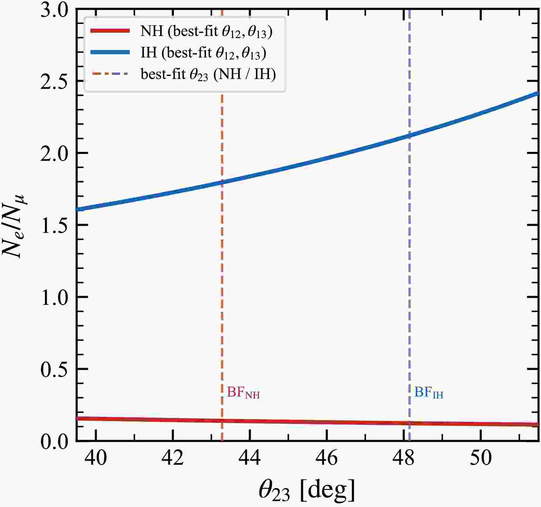
(ii) Oscillation-parameter uncertainties. Scanning $ 5 \times 10^4 $ points uniformly over the NUFIT 6.1 $ 3\sigma $ ranges ($ \theta_{12} \in [32.54^\circ, 35.03^\circ] $, $ \theta_{13} \in [8.27^\circ, 8.95^\circ] $, $ \theta_{23} \in [41.11^\circ, 50.02^\circ] $) [2] at $ m_{{\rm{lightest}}} = 0 $ yields NH: $ N_e/ N_\mu \in [0.099, 0.181] $ and IH: $ [1.602, 2.490] $. Even for the most unfavorable parameter combination—the IH minimum (1.602) and the NH maximum (0.181)—the discrimination ratio remains as large as $ {\cal{R}} = 8.85 $ (smaller than earlier estimates that used a single $ \theta_{23} $ value for both hierarchies, because here each hierarchy is evaluated at its own NuFit 6.1 best-fit $ \theta_{23} $). As oscillation experiments further constrain $ \theta_{23} $, this gap widens rather than narrows (Fig. 1).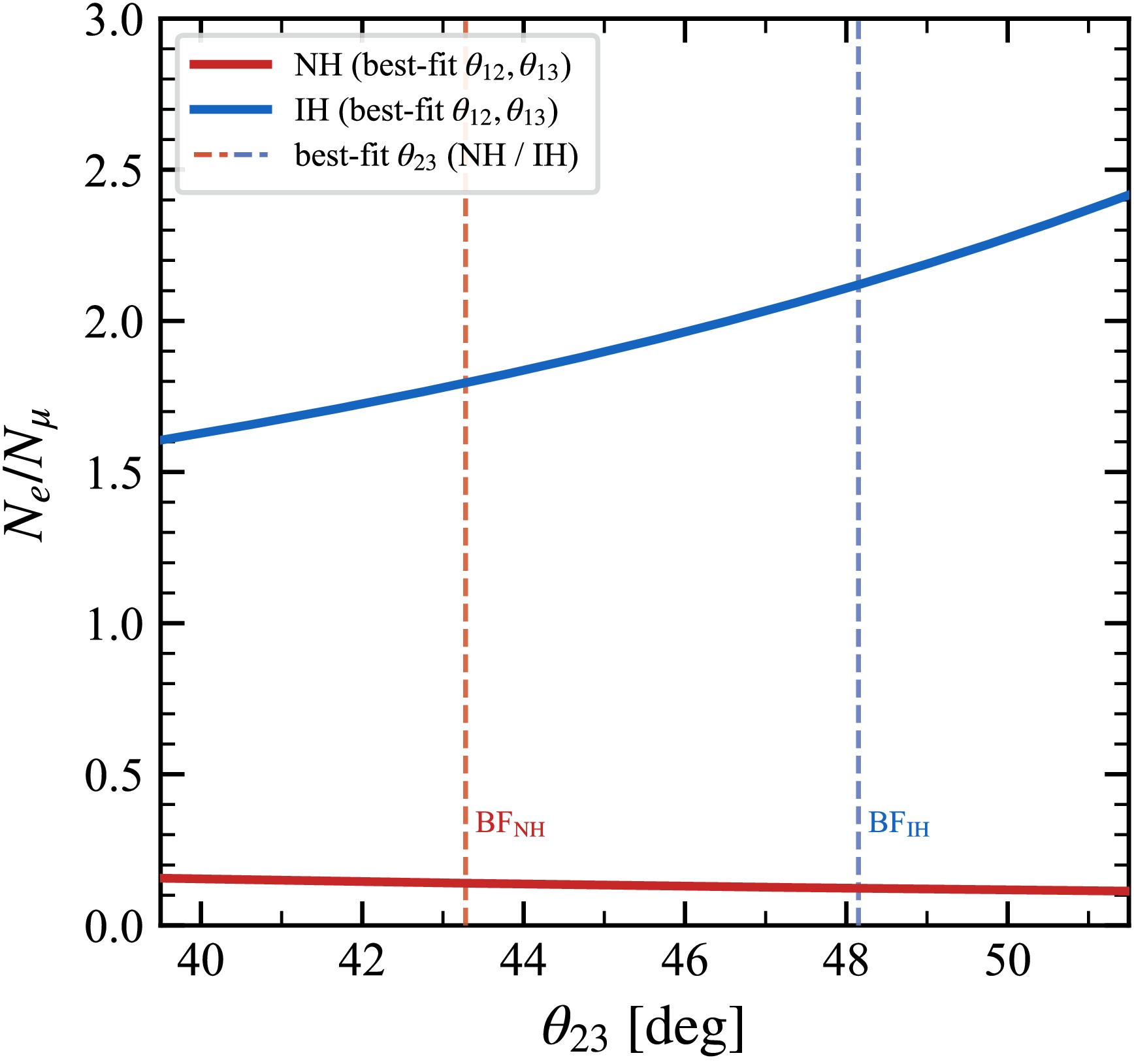

Figure 1.  (color online) Predicted $ N_e/ N_\mu $ for NH (red) and IH (blue) as a function of $ \theta_{23} $, evaluated at the NUFIT 6.1 best-fit values of $ \theta_{12} $ and $ \theta_{13} $ [2]. Vertical dashed lines indicate the NUFIT 6.1 best-fit values of $ \theta_{23} $ for NH ($ 43.3^\circ $) and IH ($ 48.2^\circ $). Across the full $ 3\sigma $ range of $ \theta_{23} $, the two curves remain separated by more than the global worst-case value $ {\cal{R}} = 8.85 $. This value is attained only in the full three-angle $ 3\sigma $ scan described in the text; improved oscillation measurements will further sharpen the discrimination.

(iii) Lightest neutrino mass. The full dependence of $ N_e/ N_\mu $ on $ m_{{\rm{lightest}}} $ is presented in Appendix A. Within the conservative Planck 2018 bound [32] ($ \sum_i m_i \lt 120\; {\rm{meV}} $; the DESI BAO constraint [33] is tighter but depends on the cosmological combination, so we adopt Planck 2018 as the conservative baseline), the IH prediction does not fall below $ {\approx}1.58 $ (reached at its Planck-allowed maximum $ m_{{\rm{lightest}}} \approx 15\; {\rm{meV}} $), whereas the NH prediction rises to at most 0.71 (at $ m_{{\rm{lightest}}} \approx 30\; {\rm{meV}} $); the discrimination ratio therefore satisfies $ {\cal{R}} \geq 2.2 $ ($ \approx 1.58/0.71 $) throughout the Planck-allowed range. In practice, current cosmological fits and the direct upper limit $ m_\nu \lt 0.45\; {\rm{eV}} $ from KATRIN [34] are consistent with $ m_{{\rm{lightest}}} \lesssim 15\; {\rm{meV}} $, for which the discrimination ratio satisfies $ {\cal{R}} \gt 2.9 $.

(iv) Non-degenerate mediator masses. A scan over non-degenerate right-handed-neutrino spectra in the Scotogenic model, with mass splittings up to 50%, shows that the discrimination ratio satisfies $ {\cal{R}} \gt 9 $ in all cases (Appendix B).

(v) R-matrix freedom. For real orthogonal R, $ \sum_i |y_{i\alpha}|^2 $ is independent of R, and Eq. (1) holds exactly. In the parameter space compatible with the MEG II bound [35] ($ {\rm{BR}}(\mu\to e\gamma) \lt 1.5\times10^{-13} $), a scan over $ 10^5 $ complex-R matrices shows deviations of at most $ {\cal{O}}$(10–30%) in $ N_e/ N_\mu $—far below the factor $ {\cal{R}} = 15.1 $ separating the NH and IH predictions (see Appendix B for scan details).

(vi) Detector efficiency. At the detector level, the measured ratio differs from the theoretical prediction by the relative efficiency $ r_\varepsilon \equiv \langle\varepsilon_e\rangle/\langle\varepsilon_\mu\rangle $:

Because $ r_\varepsilon $ appears as a common multiplicative factor, it cancels exactly in the NH–IH separation: $ (N_e/N_\mu)^{{\rm{IH}}}_{{\rm{det}}} / (N_e/N_\mu)^{{\rm{NH}}}_{{\rm{det}}} = {\cal{R}} = 15.1 $ for any $ r_\varepsilon \gt 0 $. Figure 2 illustrates this behavior: on a log–log scale, the NH and IH lines are parallel with unit slope and are separated by $ \log {\cal{R}} $, with the hierarchy-decision threshold $ r_\varepsilon \times 0.543 $, derived in Sec. V, lying between them for all $ r_\varepsilon \gt 0 $. The value of $ r_\varepsilon $ can be measured using a displaced-lepton control sample; suitable candidates include displaced $ J/\psi \to \ell^+\ell^- $ decays reconstructed in the timing layer, which share the same lepton-identification and timing-selection chain as the signal without requiring any BSM model input [10]. The same control sample also constrains the flavor asymmetry of any residual background, as discussed in Sec. V. Applying Eq. (9) therefore does not require a model-specific full-detector reinterpretation of the BSM signal.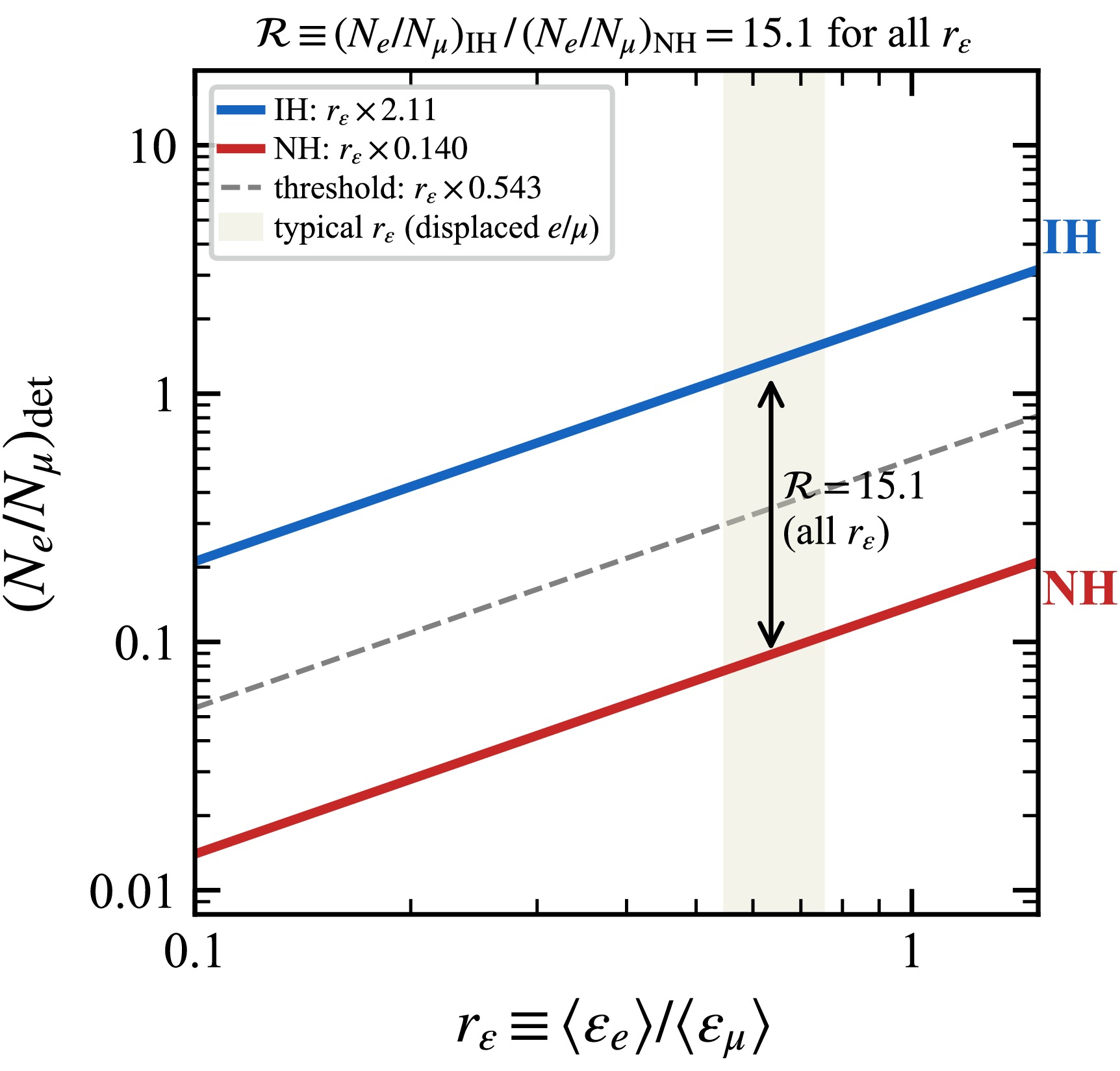

Figure 2.  (color online) Detector-level ratio $ (N_e/N_\mu)_{{\rm{det}}} $ vs. $ r_\varepsilon \equiv \langle\varepsilon_e\rangle/\langle\varepsilon_\mu\rangle $ for NH (red; theory value 0.140) and IH (blue; theory value 2.11). Both lines have unit slope on the log–log scale, reflecting the exact cancellation of $ r_\varepsilon $ in Eq. (9), with a constant separation of $ {\cal{R}} = 15.1 $ for any $ r_\varepsilon \gt 0 $. The dashed gray line shows the hierarchy-decision threshold, $ r_\varepsilon \times 0.543 $, derived in Sec. V; it lies between the two lines for all $ r_\varepsilon \gt 0 $. Olive band: typical displaced-track regime, $ r_\varepsilon \approx 0.55 $–0.75, at ATLAS and CMS. Theory inputs: NUFIT 6.1 best fit [2], $ m_{{\rm{lightest}}} = 0 $, with each hierarchy evaluated at its own best-fit parameters (Table 1).

Six potential sources of uncertainty—the CP phase, the measured oscillation parameters, the absolute neutrino mass scale, the BSM mediator spectrum, the R-matrix freedom, and detector efficiencies— do not affect the hierarchy discrimination. We address each in turn.

(i) The Dirac CP phase. For real Casas–Ibarra R [condition (iii)], $ \delta_{\rm CP} $ cancels exactly in $ N_e/ N_\mu $: the observable depends on $ |U_{\alpha i}|^2 = U_{\alpha i}U_{\alpha i}^* $, which is manifestly phase-independent for fixed mixing angles and masses. The small variation seen in a numerical scan (<3% for NH, <0.5% for IH) arises because NuFit's best-fit parameters $ (\theta_{ij}, \delta_{\rm CP}) $ are jointly determined from global data. Thus, scanning $ \delta_{\rm CP} $ at the corresponding best-fit $ \theta_{ij} $ values introduces an indirect correlation, rather than a genuine phase dependence. For fixed mixing angles, the independence is exact. This is in sharp contrast to the matter-modified probability $ P(\nu_\mu \to \nu_e) $ on which long-baseline experiments rely, where the $ \delta_{\rm CP} $–hierarchy degeneracy produces $ {\cal{O}}(1) $ shifts [1]; the present observable is therefore robust against an unknown CP phase within the shared-coupling class.

(ii) Oscillation-parameter uncertainties. Scanning $ 5 \times 10^4 $ points uniformly over the NUFIT 6.1 $ 3\sigma $ ranges ($ \theta_{12} \in [32.54^\circ, 35.03^\circ] $, $ \theta_{13} \in [8.27^\circ, 8.95^\circ] $, $ \theta_{23} \in [41.11^\circ, 50.02^\circ] $) [2] at $ m_{{\rm{lightest}}} = 0 $ yields NH: $ N_e/ N_\mu \in [0.099, 0.181] $ and IH: $ [1.602, 2.490] $. Even for the most unfavorable parameter combination—the IH minimum (1.602) and the NH maximum (0.181)—the discrimination ratio remains as large as $ {\cal{R}} = 8.85 $ (smaller than earlier estimates that used a single $ \theta_{23} $ value for both hierarchies, because here each hierarchy is evaluated at its own NuFit 6.1 best-fit $ \theta_{23} $). As oscillation experiments further constrain $ \theta_{23} $, this gap widens rather than narrows (Fig. 1).

Figure 1.  (color online) Predicted $ N_e/ N_\mu $ for NH (red) and IH (blue) as a function of $ \theta_{23} $, evaluated at the NUFIT 6.1 best-fit values of $ \theta_{12} $ and $ \theta_{13} $ [2]. Vertical dashed lines indicate the NUFIT 6.1 best-fit values of $ \theta_{23} $ for NH ($ 43.3^\circ $) and IH ($ 48.2^\circ $). Across the full $ 3\sigma $ range of $ \theta_{23} $, the two curves remain separated by more than the global worst-case value $ {\cal{R}} = 8.85 $. This value is attained only in the full three-angle $ 3\sigma $ scan described in the text; improved oscillation measurements will further sharpen the discrimination.

(iii) Lightest neutrino mass. The full dependence of $ N_e/ N_\mu $ on $ m_{{\rm{lightest}}} $ is presented in Appendix A. Within the conservative Planck 2018 bound [32] ($ \sum_i m_i \lt 120\; {\rm{meV}} $; the DESI BAO constraint [33] is tighter but depends on the cosmological combination, so we adopt Planck 2018 as the conservative baseline), the IH prediction does not fall below $ {\approx}1.58 $ (reached at its Planck-allowed maximum $ m_{{\rm{lightest}}} \approx 15\; {\rm{meV}} $), whereas the NH prediction rises to at most 0.71 (at $ m_{{\rm{lightest}}} \approx 30\; {\rm{meV}} $); the discrimination ratio therefore satisfies $ {\cal{R}} \geq 2.2 $ ($ \approx 1.58/0.71 $) throughout the Planck-allowed range. In practice, current cosmological fits and the direct upper limit $ m_\nu \lt 0.45\; {\rm{eV}} $ from KATRIN [34] are consistent with $ m_{{\rm{lightest}}} \lesssim 15\; {\rm{meV}} $, for which the discrimination ratio satisfies $ {\cal{R}} \gt 2.9 $.

(iv) Non-degenerate mediator masses. A scan over non-degenerate right-handed-neutrino spectra in the Scotogenic model, with mass splittings up to 50%, shows that the discrimination ratio satisfies $ {\cal{R}} \gt 9 $ in all cases (Appendix B).

(v) R-matrix freedom. For real orthogonal R, $ \sum_i |y_{i\alpha}|^2 $ is independent of R, and Eq. (1) holds exactly. In the parameter space compatible with the MEG II bound [35] ($ {\rm{BR}}(\mu\to e\gamma) \lt 1.5\times10^{-13} $), a scan over $ 10^5 $ complex-R matrices shows deviations of at most $ {\cal{O}}$(10–30%) in $ N_e/ N_\mu $—far below the factor $ {\cal{R}} = 15.1 $ separating the NH and IH predictions (see Appendix B for scan details).

(vi) Detector efficiency. At the detector level, the measured ratio differs from the theoretical prediction by the relative efficiency $ r_\varepsilon \equiv \langle\varepsilon_e\rangle/\langle\varepsilon_\mu\rangle $:

Because $ r_\varepsilon $ appears as a common multiplicative factor, it cancels exactly in the NH–IH separation: $ (N_e/N_\mu)^{{\rm{IH}}}_{{\rm{det}}} / (N_e/N_\mu)^{{\rm{NH}}}_{{\rm{det}}} = {\cal{R}} = 15.1 $ for any $ r_\varepsilon \gt 0 $. Figure 2 illustrates this behavior: on a log–log scale, the NH and IH lines are parallel with unit slope and are separated by $ \log {\cal{R}} $, with the hierarchy-decision threshold $ r_\varepsilon \times 0.543 $, derived in Sec. V, lying between them for all $ r_\varepsilon \gt 0 $. The value of $ r_\varepsilon $ can be measured using a displaced-lepton control sample; suitable candidates include displaced $ J/\psi \to \ell^+\ell^- $ decays reconstructed in the timing layer, which share the same lepton-identification and timing-selection chain as the signal without requiring any BSM model input [10]. The same control sample also constrains the flavor asymmetry of any residual background, as discussed in Sec. V. Applying Eq. (9) therefore does not require a model-specific full-detector reinterpretation of the BSM signal.

Figure 2.  (color online) Detector-level ratio $ (N_e/N_\mu)_{{\rm{det}}} $ vs. $ r_\varepsilon \equiv \langle\varepsilon_e\rangle/\langle\varepsilon_\mu\rangle $ for NH (red; theory value 0.140) and IH (blue; theory value 2.11). Both lines have unit slope on the log–log scale, reflecting the exact cancellation of $ r_\varepsilon $ in Eq. (9), with a constant separation of $ {\cal{R}} = 15.1 $ for any $ r_\varepsilon \gt 0 $. The dashed gray line shows the hierarchy-decision threshold, $ r_\varepsilon \times 0.543 $, derived in Sec. V; it lies between the two lines for all $ r_\varepsilon \gt 0 $. Olive band: typical displaced-track regime, $ r_\varepsilon \approx 0.55 $–0.75, at ATLAS and CMS. Theory inputs: NUFIT 6.1 best fit [2], $ m_{{\rm{lightest}}} = 0 $, with each hierarchy evaluated at its own best-fit parameters (Table 1).

The $ 3\sigma $ oscillation scan in Sec. IV establishes a clear separation between the NH upper bound ($ N_e/ N_\mu \leq 0.181 $) and the IH lower bound ($ N_e/ N_\mu \geq 1.602 $). Correcting the observed ratio for efficiency using Eq. (9) yields the hierarchy decision criterion within the shared-coupling class:

where the threshold 0.543 is the geometric midpoint, $ \sqrt{(N_e/N_\mu)^{{\rm{NH}}} \cdot (N_e/N_\mu)^{{\rm{IH}}}} = \sqrt{0.140\times2.11} = 0.543 $, evaluated at $ m_{{\rm{lightest}}} = 0 $; this is a benchmark value appropriate for the cosmologically preferred regime. The criterion is valid for $ m_{{\rm{lightest}}} \lesssim 15\; {\rm{meV}} $, consistent with current cosmological constraints [32, 33]. For larger masses, the $ m_{{\rm{lightest}}} $-dependent threshold of Appendix A should be substituted, although $ m_{{\rm{lightest}}} \gtrsim 15\; {\rm{meV}} $ is disfavored, and the discrimination ratio remains $ {\cal{R}} \geq 2.2 $ throughout the Planck-allowed range.

The flavor-tomography observable is also inextricably tied to the Majorana nature of neutrino masses. If neutrinos are Dirac particles, the Casas–Ibarra relation no longer constrains the coupling to the PMNS matrix, and $ N_e/ N_\mu $ becomes a free parameter unconstrained by oscillation data. Agreement of the observed ratio with Eq. (1) would provide evidence that the LLP coupling satisfies the shared-coupling condition, consistent with Majorana mass generation. We note that this probes the coupling structure rather than the Majorana mass term directly; a definitive determination of Majorana nature additionally requires a lepton-number-violating observable such as same-sign dilepton production.

The $ 3\sigma $ oscillation scan in Sec. IV establishes a clear separation between the NH upper bound ($ N_e/ N_\mu \leq 0.181 $) and the IH lower bound ($ N_e/ N_\mu \geq 1.602 $). Correcting the observed ratio for efficiency using Eq. (9) yields the hierarchy decision criterion within the shared-coupling class:

where the threshold 0.543 is the geometric midpoint, $ \sqrt{(N_e/N_\mu)^{{\rm{NH}}} \cdot (N_e/N_\mu)^{{\rm{IH}}}} = \sqrt{0.140\times2.11} = 0.543 $, evaluated at $ m_{{\rm{lightest}}} = 0 $; this is a benchmark value appropriate for the cosmologically preferred regime. The criterion is valid for $ m_{{\rm{lightest}}} \lesssim 15\; {\rm{meV}} $, consistent with current cosmological constraints [32, 33]. For larger masses, the $ m_{{\rm{lightest}}} $-dependent threshold of Appendix A should be substituted, although $ m_{{\rm{lightest}}} \gtrsim 15\; {\rm{meV}} $ is disfavored, and the discrimination ratio remains $ {\cal{R}} \geq 2.2 $ throughout the Planck-allowed range.

The flavor-tomography observable is also inextricably tied to the Majorana nature of neutrino masses. If neutrinos are Dirac particles, the Casas–Ibarra relation no longer constrains the coupling to the PMNS matrix, and $ N_e/ N_\mu $ becomes a free parameter unconstrained by oscillation data. Agreement of the observed ratio with Eq. (1) would provide evidence that the LLP coupling satisfies the shared-coupling condition, consistent with Majorana mass generation. We note that this probes the coupling structure rather than the Majorana mass term directly; a definitive determination of Majorana nature additionally requires a lepton-number-violating observable such as same-sign dilepton production.

We estimate the signal yield for three benchmark points spanning the LLP mass range in Table 2, using the Scotogenic model as a concrete example. The $ pp \to \tilde{\eta}^{+}\tilde{\eta}^{-} $ production cross section at $ \sqrt{s} = 14\; {\rm{TeV}} $ is computed at LO with MADGRAPH5_AMC@NLO 3.5.13 [36] using the $\mathrm{InertDoublet}\_\mathrm{UFO}$ model [37, 38] and $\mathrm{NNPDF2.3LO}$ PDFs [39], yielding $ \sigma_{{\rm{LO}}} = 3.66\; {\rm{fb}} $ ($ M_{{\rm{LLP}}} = 300\; {\rm{GeV}} $), $ 1.09\; {\rm{fb}} $ ($ 400\; {\rm{GeV}} $), and $ 0.165\; {\rm{fb}} $ ($ 600\; {\rm{GeV}} $). Applying an NLO K-factor of $ K \approx 1.3 $, consistent with NLO QCD calculations for color-singlet scalar pair production via Drell–Yan in this mass range [40, 41], gives $ \sigma_{{\rm{NLO}}} = 4.76 $, 1.41, and $ 0.214\; {\rm{fb}} $, respectively. With $ {\cal{L}} = 3000\; {\rm{fb}}^{-1} $ and a representative combined efficiency $ \epsilon_{{\rm{sel}}} $ ≈ 5–10%, estimated from the geometric acceptance of the timing layer [10, 11], the $ \Delta t \gt 200\; {\rm{ps}} $ signal fraction for $ M_{{\rm{LLP}}} \sim 300{-} 600\; {\rm{GeV}} $ [42, 43], and the displaced-lepton reconstruction efficiency reported in the MTD and HGTD TDRs [10, 11], the expected number of timing-tagged $ e/\mu $ displaced leptons—with the τ channel, which carries no prompt $ e/\mu $ tag, absorbed into $ \epsilon_{{\rm{sel}}} $ as signal loss—is $ N_{{\rm{disp}}} = 2\,\sigma_{{\rm{NLO}}}\,{\cal{L}}\,\epsilon_{{\rm{sel}}} $, where the factor of 2 accounts for the decay of both $ \tilde\eta^+ $ and $ \tilde\eta^- $ in each pair-production event: $ N_{{\rm{disp}}} \approx 1430\text{–}2856 $, $ 424\text{–}846 $, and $ 64\text{–}128 $ for the three mass points, respectively.

We estimate the signal yield for three benchmark points spanning the LLP mass range in Table 2, using the Scotogenic model as a concrete example. The $ pp \to \tilde{\eta}^{+}\tilde{\eta}^{-} $ production cross section at $ \sqrt{s} = 14\; {\rm{TeV}} $ is computed at LO with MADGRAPH5_AMC@NLO 3.5.13 [36] using the $\mathrm{InertDoublet}\_\mathrm{UFO}$ model [37, 38] and $\mathrm{NNPDF2.3LO}$ PDFs [39], yielding $ \sigma_{{\rm{LO}}} = 3.66\; {\rm{fb}} $ ($ M_{{\rm{LLP}}} = 300\; {\rm{GeV}} $), $ 1.09\; {\rm{fb}} $ ($ 400\; {\rm{GeV}} $), and $ 0.165\; {\rm{fb}} $ ($ 600\; {\rm{GeV}} $). Applying an NLO K-factor of $ K \approx 1.3 $, consistent with NLO QCD calculations for color-singlet scalar pair production via Drell–Yan in this mass range [40, 41], gives $ \sigma_{{\rm{NLO}}} = 4.76 $, 1.41, and $ 0.214\; {\rm{fb}} $, respectively. With $ {\cal{L}} = 3000\; {\rm{fb}}^{-1} $ and a representative combined efficiency $ \epsilon_{{\rm{sel}}} $ ≈ 5–10%, estimated from the geometric acceptance of the timing layer [10, 11], the $ \Delta t \gt 200\; {\rm{ps}} $ signal fraction for $ M_{{\rm{LLP}}} \sim 300{-} 600\; {\rm{GeV}} $ [42, 43], and the displaced-lepton reconstruction efficiency reported in the MTD and HGTD TDRs [10, 11], the expected number of timing-tagged $ e/\mu $ displaced leptons—with the τ channel, which carries no prompt $ e/\mu $ tag, absorbed into $ \epsilon_{{\rm{sel}}} $ as signal loss—is $ N_{{\rm{disp}}} = 2\,\sigma_{{\rm{NLO}}}\,{\cal{L}}\,\epsilon_{{\rm{sel}}} $, where the factor of 2 accounts for the decay of both $ \tilde\eta^+ $ and $ \tilde\eta^- $ in each pair-production event: $ N_{{\rm{disp}}} \approx 1430\text{–}2856 $, $ 424\text{–}846 $, and $ 64\text{–}128 $ for the three mass points, respectively.

To distinguish NH from IH at $ 3\sigma $ confidence, we use an exact one-sided Poisson test based on the observed electron count $ N_e $. At $ N_{{\rm{disp}}} = 25 $, NH predicts $ (N_e, N_\mu) = (3.1, 21.9) $, while IH predicts $ (17.0, 8.0) $. The exact Poisson probability of observing $ N_e \leq 3 $ given the IH expectation of 17.0 is $ p = 8.6 \times 10^{-5} $ ($ 3.8\sigma $), and the reverse misclassification probability is $ p = 2.1 \times 10^{-7} $ ($ 5.1\sigma $). Hence, $ {\cal{O}}(25) $ events provide $ 3\sigma $ discrimination in an ideal Poisson counting experiment. A few-percent systematic uncertainty on $ r_\varepsilon $, which can be measured from the displaced $ J/\psi \to \ell^+\ell^- $ control sample of Sec. IV, shifts $ (N_e/N_\mu)^{{\rm{obs}}} $ by far less than the factor $ {\cal{R}} = 15.1 $ separating the predictions and therefore does not materially increase this threshold. A complementary binomial test, conditioning on the total $ e+\mu $ count and profiling over the $ r_\varepsilon $ uncertainty, is presented in Appendix C. Both statistical frameworks give $ \geq 3\sigma $ at $ {\cal{O}}(10) $ events, confirming that the result is robust to the choice of test. Even the most challenging $ 600\; {\rm{GeV}} $ benchmark accumulates $ N_{{\rm{disp}}} \approx $ 64–128 and yields a Poisson p-value below 0.003 for the wrong hierarchy, confirming that the criterion of Eq. (10) is satisfied across the full LLP mass range at HL-LHC luminosity.

To distinguish NH from IH at $ 3\sigma $ confidence, we use an exact one-sided Poisson test based on the observed electron count $ N_e $. At $ N_{{\rm{disp}}} = 25 $, NH predicts $ (N_e, N_\mu) = (3.1, 21.9) $, while IH predicts $ (17.0, 8.0) $. The exact Poisson probability of observing $ N_e \leq 3 $ given the IH expectation of 17.0 is $ p = 8.6 \times 10^{-5} $ ($ 3.8\sigma $), and the reverse misclassification probability is $ p = 2.1 \times 10^{-7} $ ($ 5.1\sigma $). Hence, $ {\cal{O}}(25) $ events provide $ 3\sigma $ discrimination in an ideal Poisson counting experiment. A few-percent systematic uncertainty on $ r_\varepsilon $, which can be measured from the displaced $ J/\psi \to \ell^+\ell^- $ control sample of Sec. IV, shifts $ (N_e/N_\mu)^{{\rm{obs}}} $ by far less than the factor $ {\cal{R}} = 15.1 $ separating the predictions and therefore does not materially increase this threshold. A complementary binomial test, conditioning on the total $ e+\mu $ count and profiling over the $ r_\varepsilon $ uncertainty, is presented in Appendix C. Both statistical frameworks give $ \geq 3\sigma $ at $ {\cal{O}}(10) $ events, confirming that the result is robust to the choice of test. Even the most challenging $ 600\; {\rm{GeV}} $ benchmark accumulates $ N_{{\rm{disp}}} \approx $ 64–128 and yields a Poisson p-value below 0.003 for the wrong hierarchy, confirming that the criterion of Eq. (10) is satisfied across the full LLP mass range at HL-LHC luminosity.

A crucial feature of the flavor-ratio observable is its resilience to any prompt background that survives the timing cut: because the hierarchy is encoded in $ N_e/N_\mu $ rather than in an absolute rate, a flavor-symmetric residual—contributing equally to the e and μ counts—can only drive the measured ratio toward unity and dilute the discrimination; it can never reverse the direction of the NH–IH separation. Only a flavor-asymmetric residual can bias the assignment, and it must therefore be controlled at the few-percent level using the same displaced $ J/\psi \to \ell^+\ell^- $ control sample that determines $ r_\varepsilon $ (Sec. IV). Under the conservative working assumption that the data-driven timing sidebands suppress the prompt background to $ \lesssim $10% of the signal, with $ e/\mu $ asymmetry below the few-percent level, the separation degrades by less than $ {\cal{O}}(1) $, and the decision criterion of Eq. (10) is preserved; a quantitative background estimate based on a full detector simulation is left to a dedicated experimental study.

A crucial feature of the flavor-ratio observable is its resilience to any prompt background that survives the timing cut: because the hierarchy is encoded in $ N_e/N_\mu $ rather than in an absolute rate, a flavor-symmetric residual—contributing equally to the e and μ counts—can only drive the measured ratio toward unity and dilute the discrimination; it can never reverse the direction of the NH–IH separation. Only a flavor-asymmetric residual can bias the assignment, and it must therefore be controlled at the few-percent level using the same displaced $ J/\psi \to \ell^+\ell^- $ control sample that determines $ r_\varepsilon $ (Sec. IV). Under the conservative working assumption that the data-driven timing sidebands suppress the prompt background to $ \lesssim $10% of the signal, with $ e/\mu $ asymmetry below the few-percent level, the separation degrades by less than $ {\cal{O}}(1) $, and the decision criterion of Eq. (10) is preserved; a quantitative background estimate based on a full detector simulation is left to a dedicated experimental study.

The key structural observation of this Letter is that the $ \delta_{\rm CP} $–hierarchy degeneracy that affects all long-baseline oscillation programs is absent in the flavor-tomography observable: $ N_e/ N_\mu $ depends on $ |U_{\alpha i}|^2 $, not on $ U_{\alpha i} $, so no value of $ \delta_{\rm CP} $ can shift the NH prediction (0.140) toward the IH prediction (2.11) within the shared-coupling class. Instead, the hierarchy is encoded in a ratio of lepton counts determined entirely by already measured oscillation parameters, robust against $ {\cal{O}}(1) $ variations in detector efficiency, and insensitive to BSM mass parameters. This method is complementary to JUNO [6, 7]: both approaches are $ \delta_{\rm CP} $-independent and can operate in the same era, but flavor tomography directly probes the Majorana coupling structure of the LLP mediator, a dimension not addressed by oscillation or reactor measurements. We have verified the prediction across four representative BSM model classes. Analytically, it is traceable to $ 2\tan^2\theta_{13} $ (NH) and $ {\approx}1.9 $ at maximal mixing (IH; exact value 2.11), with a discrimination ratio no smaller than $ {\cal{R}} = 8.85 $ across the full $ 3\sigma $ oscillation band and $ {\cal{R}} \geq 2.2 $ within the cosmologically allowed mass ranges [32, 33]. The prediction will become only sharper as oscillation measurements improve.

The key structural observation of this Letter is that the $ \delta_{\rm CP} $–hierarchy degeneracy that affects all long-baseline oscillation programs is absent in the flavor-tomography observable: $ N_e/ N_\mu $ depends on $ |U_{\alpha i}|^2 $, not on $ U_{\alpha i} $, so no value of $ \delta_{\rm CP} $ can shift the NH prediction (0.140) toward the IH prediction (2.11) within the shared-coupling class. Instead, the hierarchy is encoded in a ratio of lepton counts determined entirely by already measured oscillation parameters, robust against $ {\cal{O}}(1) $ variations in detector efficiency, and insensitive to BSM mass parameters. This method is complementary to JUNO [6, 7]: both approaches are $ \delta_{\rm CP} $-independent and can operate in the same era, but flavor tomography directly probes the Majorana coupling structure of the LLP mediator, a dimension not addressed by oscillation or reactor measurements. We have verified the prediction across four representative BSM model classes. Analytically, it is traceable to $ 2\tan^2\theta_{13} $ (NH) and $ {\approx}1.9 $ at maximal mixing (IH; exact value 2.11), with a discrimination ratio no smaller than $ {\cal{R}} = 8.85 $ across the full $ 3\sigma $ oscillation band and $ {\cal{R}} \geq 2.2 $ within the cosmologically allowed mass ranges [32, 33]. The prediction will become only sharper as oscillation measurements improve.

Figure A1 shows $ N_e/ N_\mu $ as a function of $ m_{{\rm{lightest}}} $. Both hierarchies converge to the common asymptotic value $ N_e/ N_\mu \to 1 $ as the spectrum becomes quasi-degenerate ($ m_{{\rm{lightest}}} \gg 50\; {\rm{meV}} $), because equal-mass eigenstates weight each flavor by the unitary row sum $ \sum_i |U_{\alpha i}|^2 = 1 $, causing the flavor-weighted mass sums $ {\cal{A}}_e $ and $ {\cal{A}}_\mu $ to become equal. We adopt the conservative Planck 2018 bound [32] $ \sum m_i \lt 120\; {\rm{meV}} $; the DESI BAO constraint [33] is tighter but depends on the cosmological data combination. Within this window, the IH prediction remains at or above $ {\approx}1.58 $ (reached at its Planck-allowed maximum $ m_{{\rm{lightest}}} \approx 15\; {\rm{meV}} $), whereas the NH prediction rises to at most 0.71 (at $ m_{{\rm{lightest}}} \approx 30\; {\rm{meV}} $). Thus, the discrimination ratio satisfies $ {\cal{R}} \geq 2.2 $ throughout the Planck-allowed range. For $ m_{{\rm{lightest}}} \gtrsim 15\; {\rm{meV}} $, the $ m_{{\rm{lightest}}} $-dependent geometric-midpoint threshold, $ \sqrt{(N_e/N_\mu)^{{\rm{NH}}} (N_e/N_\mu)^{{\rm{IH}}}} $ evaluated at the relevant $ m_{{\rm{lightest}}} $, replaces the benchmark value 0.543 in Eq. (10). Defining $ m_*(f) $ as the lightest mass at which the IH-to-NH ratio, evaluated at a common $ m_{{\rm{lightest}}} $, equals f, one finds $ m_*(f{=}2) \approx 27\; {\rm{meV}} $ (just beyond the IH Planck-allowed range) and $ m_*(f{=}10) \approx 2.4\; {\rm{meV}} $ (comfortably above current NH oscillation fits [2] and the KATRIN direct limit [34]).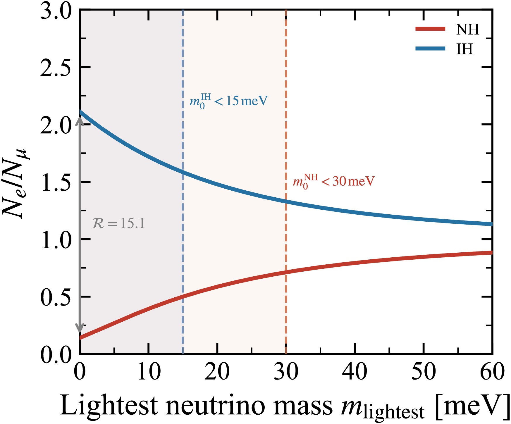

Figure A1.  (color online) Predicted $ N_e/ N_\mu $ as a function of $ m_{{\rm{lightest}}} $ for NH (red) and IH (blue), assuming the NUFIT 6.1 best-fit mixing angles [2]. The vertical dashed lines indicate the Planck 2018 [32] upper bounds ($ {<}30\; {\rm{meV}} $ for NH and $ {<}15\; {\rm{meV}} $ for IH). At the Planck boundaries, the IH prediction is 1.58 (at $ 15\; {\rm{meV}} $), and the NH prediction is 0.71 (at $ 30\; {\rm{meV}} $); therefore, the discrimination ratio satisfies $ {\cal{R}} \geq 2.2 $ throughout the allowed region. The critical mass $ m_*(f{=}2) \approx 27\; {\rm{meV}} $ lies within the Planck-allowed NH range. Both hierarchies approach the common value 1 only far beyond the Planck-allowed region. Within this region, the IH curve decreases from 2.11 at $ m_{{\rm{lightest}}}=0 $ to $ {\approx}1.58 $ at its Planck boundary, while the NH curve rises from 0.140 to 0.71.

Figure A1 shows $ N_e/ N_\mu $ as a function of $ m_{{\rm{lightest}}} $. Both hierarchies converge to the common asymptotic value $ N_e/ N_\mu \to 1 $ as the spectrum becomes quasi-degenerate ($ m_{{\rm{lightest}}} \gg 50\; {\rm{meV}} $), because equal-mass eigenstates weight each flavor by the unitary row sum $ \sum_i |U_{\alpha i}|^2 = 1 $, causing the flavor-weighted mass sums $ {\cal{A}}_e $ and $ {\cal{A}}_\mu $ to become equal. We adopt the conservative Planck 2018 bound [32] $ \sum m_i \lt 120\; {\rm{meV}} $; the DESI BAO constraint [33] is tighter but depends on the cosmological data combination. Within this window, the IH prediction remains at or above $ {\approx}1.58 $ (reached at its Planck-allowed maximum $ m_{{\rm{lightest}}} \approx 15\; {\rm{meV}} $), whereas the NH prediction rises to at most 0.71 (at $ m_{{\rm{lightest}}} \approx 30\; {\rm{meV}} $). Thus, the discrimination ratio satisfies $ {\cal{R}} \geq 2.2 $ throughout the Planck-allowed range. For $ m_{{\rm{lightest}}} \gtrsim 15\; {\rm{meV}} $, the $ m_{{\rm{lightest}}} $-dependent geometric-midpoint threshold, $ \sqrt{(N_e/N_\mu)^{{\rm{NH}}} (N_e/N_\mu)^{{\rm{IH}}}} $ evaluated at the relevant $ m_{{\rm{lightest}}} $, replaces the benchmark value 0.543 in Eq. (10). Defining $ m_*(f) $ as the lightest mass at which the IH-to-NH ratio, evaluated at a common $ m_{{\rm{lightest}}} $, equals f, one finds $ m_*(f{=}2) \approx 27\; {\rm{meV}} $ (just beyond the IH Planck-allowed range) and $ m_*(f{=}10) \approx 2.4\; {\rm{meV}} $ (comfortably above current NH oscillation fits [2] and the KATRIN direct limit [34]).

Figure A1.  (color online) Predicted $ N_e/ N_\mu $ as a function of $ m_{{\rm{lightest}}} $ for NH (red) and IH (blue), assuming the NUFIT 6.1 best-fit mixing angles [2]. The vertical dashed lines indicate the Planck 2018 [32] upper bounds ($ {<}30\; {\rm{meV}} $ for NH and $ {<}15\; {\rm{meV}} $ for IH). At the Planck boundaries, the IH prediction is 1.58 (at $ 15\; {\rm{meV}} $), and the NH prediction is 0.71 (at $ 30\; {\rm{meV}} $); therefore, the discrimination ratio satisfies $ {\cal{R}} \geq 2.2 $ throughout the allowed region. The critical mass $ m_*(f{=}2) \approx 27\; {\rm{meV}} $ lies within the Planck-allowed NH range. Both hierarchies approach the common value 1 only far beyond the Planck-allowed region. Within this region, the IH curve decreases from 2.11 at $ m_{{\rm{lightest}}}=0 $ to $ {\approx}1.58 $ at its Planck boundary, while the NH curve rises from 0.140 to 0.71.

Non-degenerate right-handed-neutrino masses. In the Scotogenic model, non-degenerate right-handed-neutrino masses introduce a loop-function weight $ {\cal{F}}(M_{N_i}/m_\eta) $ [24], thereby violating condition (ii). A scan over spectra with splittings of up to 50% confirms that the discrimination ratio satisfies $ {\cal{R}} \gt 9 $ in all cases.

Complex R-matrix. For complex $ R = e^{i\omega} $, which violates condition (iii), $ \sum_i|y_{i\alpha}|^2 $ receives corrections $ \propto \sinh^2({\rm{Im}}\,\omega_{ij}) $. The MEG II bound [35] $ {\rm{BR}}(\mu\to e\gamma) \lt 1.5\times 10^{-13} $ implies $ |{\rm{Im}}\,\omega_{12}|\lesssim 2.5 $ ($ M_N\sim 1\; {\rm{TeV}} $). A scan over $ 10^5 $ matrices satisfying this bound yields deviations of $ {\cal{O}}$(10%) in $ N_e/ N_\mu $, far below the factor $ {\cal{R}} = 15.1 $ separating the hierarchy predictions. In the less constrained $ e\tau/\mu\tau $ subspace, the deviations reach $ {\cal{O}}$(30%), still well within the gap.

τ contamination. Three suppression factors keep τ-induced $ e/\mu $ contamination at $ \lesssim $0.5%: the leptonic τ sub-branching ratios ($ \approx $18% and 17%), the $ {\cal{O}}(10^{-2}) $ probability that a secondary lepton from $ \tau\to\ell\nu\bar\nu $ ($ c\tau_\tau\approx 87\; \mu{\rm{m}} $) passes the $ \Delta t>200\; {\rm{ps}} $ cut, and standard displaced-track veto requirements.

Non-degenerate right-handed-neutrino masses. In the Scotogenic model, non-degenerate right-handed-neutrino masses introduce a loop-function weight $ {\cal{F}}(M_{N_i}/m_\eta) $ [24], thereby violating condition (ii). A scan over spectra with splittings of up to 50% confirms that the discrimination ratio satisfies $ {\cal{R}} \gt 9 $ in all cases.

Complex R-matrix. For complex $ R = e^{i\omega} $, which violates condition (iii), $ \sum_i|y_{i\alpha}|^2 $ receives corrections $ \propto \sinh^2({\rm{Im}}\,\omega_{ij}) $. The MEG II bound [35] $ {\rm{BR}}(\mu\to e\gamma) \lt 1.5\times 10^{-13} $ implies $ |{\rm{Im}}\,\omega_{12}|\lesssim 2.5 $ ($ M_N\sim 1\; {\rm{TeV}} $). A scan over $ 10^5 $ matrices satisfying this bound yields deviations of $ {\cal{O}}$(10%) in $ N_e/ N_\mu $, far below the factor $ {\cal{R}} = 15.1 $ separating the hierarchy predictions. In the less constrained $ e\tau/\mu\tau $ subspace, the deviations reach $ {\cal{O}}$(30%), still well within the gap.

τ contamination. Three suppression factors keep τ-induced $ e/\mu $ contamination at $ \lesssim $0.5%: the leptonic τ sub-branching ratios ($ \approx $18% and 17%), the $ {\cal{O}}(10^{-2}) $ probability that a secondary lepton from $ \tau\to\ell\nu\bar\nu $ ($ c\tau_\tau\approx 87\; \mu{\rm{m}} $) passes the $ \Delta t>200\; {\rm{ps}} $ cut, and standard displaced-track veto requirements.

Conditioning on $ N_{e\mu} $, the total number of $ e+\mu $ events, the electron count $ K_e $ follows a binomial distribution:

with $ R_{{\rm{NH}}}=0.140 $ and $ R_{{\rm{IH}}}=2.11 $, yielding $ p_e^{{\rm{NH}}}=0.123 $ and $ p_e^{{\rm{IH}}}=0.679 $ at $ r_\varepsilon=1 $. Conditioning on the total $ e+\mu $ count makes this test insensitive to the overall signal yield, reducing it to a comparison of pure flavor fractions. Table C1 lists the one-sided misclassification p-values; the minimum $ N_{e\mu} $ required for $ 3\sigma $ significance in both directions is $ N_{e\mu}=9 $. When profiling over $ r_\varepsilon $ as a nuisance parameter, even a ±30% uncertainty in $ r_\varepsilon $ still leaves $ >4.9\sigma $ at $ N_{e\mu}=25 $, because the factor-of-5.5 difference between $ p_e^{{\rm{NH}}} $ and $ p_e^{{\rm{IH}}} $ far exceeds any $ {\cal{O}}(1) $ efficiency variation. Both this binomial test and the Poisson test of Sec. V C yield $ \geq3\sigma $ at $ {\cal{O}}(10) $ events, confirming that the result is robust to the choice of statistical framework.

Conditioning on $ N_{e\mu} $, the total number of $ e+\mu $ events, the electron count $ K_e $ follows a binomial distribution:

with $ R_{{\rm{NH}}}=0.140 $ and $ R_{{\rm{IH}}}=2.11 $, yielding $ p_e^{{\rm{NH}}}=0.123 $ and $ p_e^{{\rm{IH}}}=0.679 $ at $ r_\varepsilon=1 $. Conditioning on the total $ e+\mu $ count makes this test insensitive to the overall signal yield, reducing it to a comparison of pure flavor fractions. Table C1 lists the one-sided misclassification p-values; the minimum $ N_{e\mu} $ required for $ 3\sigma $ significance in both directions is $ N_{e\mu}=9 $. When profiling over $ r_\varepsilon $ as a nuisance parameter, even a ±30% uncertainty in $ r_\varepsilon $ still leaves $ >4.9\sigma $ at $ N_{e\mu}=25 $, because the factor-of-5.5 difference between $ p_e^{{\rm{NH}}} $ and $ p_e^{{\rm{IH}}} $ far exceeds any $ {\cal{O}}(1) $ efficiency variation. Both this binomial test and the Poisson test of Sec. V C yield $ \geq3\sigma $ at $ {\cal{O}}(10) $ events, confirming that the result is robust to the choice of statistical framework.