Nuclear mass models with deformation optimized and diagnosed by Bayesian analysis with Markov chain Monte Carlo

The Bethe-Weizsäcker semi-empirical mass formula [1, 2] expresses the liquid-drop model (LDM) first suggested by Gamow [3]. After its systematic refinement by Bethe and Bacher [2], early pioneers such as Meitner and Frisch [4] used the LDM to explain the newly discovered fission reported by Hahn and Strassmann [5]. Later, the community used this mass model to predict a wide range of nuclear binding energies beyond the reach of contemporary experiments. The Bethe-Weizsäcker (BW) mass model assumes the nucleus to be a very high-density drop of incompressible fluid, with its nucleons held together by the nuclear force. The BW model is characterized by several physical terms, namely volume, surface, Coulomb, and symmetry energies, and has become one of the classic phenomenological models despite its inability to describe binding energies in regions of the historical magic numbers. The strengths of these physical terms have been continually updated through least-squares fitting (and subsequent refinements) using contemporary experimental data, e.g., Evans [6], Gunter and Hubbs [7], Bauer and Canuto [8], Myers [9], Tseng et al. [10], Eisberg and Resnick [11], Rohlf [12], Samanta and Adhikari [13], Kirson [14], Mavrodiev and Vol [15], Gjorgievska et al. [16], and Wu et al. [17]. Numerous further refinements have been made since the work of Bethe and Bacher. For instance, Spanier and Johansson [18] added empirical deformation and shell corrections to the BW model, whereas Kirson [14] refined the model by introducing several new terms, i.e., Coulomb exchange, Wigner, pairing, surface symmetry, and curvature energies, as well as shell correction. More recently, Wu et al. [17] adopted the isospin-dependent symmetry-energy term with surface diffuseness from the WS4 model [19], reconstructed the symmetry-energy term, and introduced regional shell corrections. They then formulated the BWN mass model, which significantly reduces the discrepancy between experimental and theoretical binding energies, achieving a root-mean-square deviation of 887 keV. Although all these refinements improve upon the original BW mass model, these new BW-variant mass models still exhibit noticeable systematic deviations in strongly deformed regions, especially in the rare-earth region.

Recent remarkable advances in experimental techniques have laid the foundation for the establishment of state-of-the-art radioactive isotope beam facilities, opening unprecedented opportunities to synthesize very short-lived nuclei far from the valley of stability [20, 21], e.g., the Facility for Rare Isotope Beams (FRIB) in the US [22], the Radioactive Ion Beam Factory (RIBF) at RIKEN in Japan [23], the Second Generation System On-Line Production of Radioactive Ions (SPIRAL2) at GANIL in France [24], the recently commissioned High-Intensity Heavy-Ion Accelerator Facility (HIAF) in China [25], and the currently under-construction Facility for Antiproton and Ion Research (FAIR) in Germany [26] and the Rare Isotope Accelerator complex for Online Experiments (RAON) in Korea [27].

Nevertheless, many exotic nuclei of great interest in nuclear astrophysics remain beyond the reach of these facilities. Hence, robust and cost-effective nuclear mass models capable of precisely predicting binding energies across a wide range of nuclei are needed, providing (i) prior information for experimental measurements [28], (ii) an essential basis for constructing macroscopic-microscopic approaches, which implicitly account for quantum shell effects, e.g., the WS3 and WS4 models [19, 29], (iv) high-precision training databases for developing artificial intelligence (AI) mass models [30−33], (v) interpretable physical features for physics-informed AI approaches [34−36], (vi) determination of the proton drip line, which is important for studying the rapid-proton capture process [37−46], (vii) single- and two-neutron separation energies indispensable for (n,γ) and (2n,γ) reaction rates in investigations of the rapid neutron-capture process [47−54], and (viii) a leading reference for mass compilations using microphysics approaches, e.g., binding energies based on the relativistic Hartree-Bogoliubov approach [55] with PC-X [56], PC-L3R [57], DD-PCX [58], and DD-MEX [56] interactions and the relativistic Hartree-Bogoliubov approach in continuum [59, 60] with the PC-PK1 interaction [61].

The construction of robust and cost-effective mass models involves refining the classical BW model either by introducing new terms in addition to the original ones and modifying these new terms, or by refitting the strengths (or parameters) of the original terms using new experimental inputs. All of these procedures employ least-squares fitting to optimize the parameters. Although the least-squares fitting method can be applied to estimate parameters of nonlinear models, it inherently relies on local linear approximations and can provide only point estimates and asymptotic standard errors [62, 63]. Moreover, it does not accurately capture the actual uncertainty of the parameters. The approximated errors can be substantial, especially when the sample size is limited or the model is highly nonlinear. In fact, the classical BW model and its variants are formulated as nonlinear functions calibrated with parameters and coefficients that depend on the mass number and proton number. The parameter space exhibits strong nonlinearity and multiscale features, resulting in a complex mapping between binding energy and the mass and proton numbers.

Bayesian inference offers an alternative for exploring the parameter space. By treating unknown parameters as random variables and combining prior information with the likelihood of the observed data, it yields the full posterior distribution, which quantifies all sources of uncertainty. This posterior distribution directly reflects the nonlinear structure of the model without requiring linearization and provides a complete description of parameter uncertainty, including correlations among parameters [64−69].

For BW-variant mass models, the parameters are physically correlated. For instance, the volume and surface coefficients may exhibit a compensatory effect when fitting nuclear masses. The least-squares fitting method can provide only point estimates and marginal confidence intervals, and even when a covariance matrix is computed, it is based on local linear approximations (e.g., the inverse of the Fisher information matrix and maximum likelihood estimation), which can be distorted in nonlinear models [70−74]. In this setting, the Bayesian posterior distribution naturally encodes the joint dependencies among parameters. By studying the posterior, one can obtain samples that reveal the correlation structure, enabling accurate estimation of correlations between any two parameters, including nonlinear dependencies. This is crucial for understanding the physical meaning of the model, diagnosing parameter degeneracy, and performing subsequent uncertainty propagation [64−69].

Bayesian analysis with the Markov chain Monte Carlo sampling method. In the Bayesian framework, when the model is complex, the parameter dimension is high, and the likelihood function has a complicated form, the posterior distribution cannot be obtained directly by analytical methods. The Markov chain Monte Carlo (MCMC) sampling method generates approximately independent samples from the target posterior distribution to support subsequent statistical inference. Its advantages include (i) handling complex and high-dimensional posterior distributions [64, 65, 67, 75], (ii) avoiding linear approximations and thus preventing the introduction of unknown errors [64, 65, 76], (iii) fully characterizing uncertainty [64, 65, 67], (iv) revealing parameter correlation structures through posterior distributions [64, 65, 76], and (v) being applicable to various complex models, e.g., hierarchical models and state-space models [67, 76, 77].

A critical yet overlooked limitation in available nuclear-mass uncertainty quantification is the use of linear correlation diagnostics to analyze inherently nonlinear parameter landscapes. For instance, the recent work by Xu et al. [78] assumed that the collinearity of a 12-parameter LDM could be analyzed using Pearson correlation coefficients, which generated a large condition number and led them to conclude that the parameter space was not properly constrained; they then implemented L2 regularization to constrain the coefficients. In fact, such a large condition number is an artifact of the assumed linearity in the parameter space. For BW-variant mass models, parameter compensation manifests nonlinear characteristics; however, the Pearson correlation coefficient is suitable only for representing the degree of linear correlation among parameters. In this case, using the Spearman rank-correlation matrix (rank transform method) [79−81] is more appropriate for analyzing nonlinear correlations among the parameters of a mass model.

Nuclear mass model with deformation. Almost all previous BW-variant mass models do not take into account the essential effect of nuclear deformation; i.e., the nuclei are assumed to be spherical. For instance, the model of Kirson [14] consists of several higher-order terms but does not account for the contribution of equilibrium deformation to the binding energy, whereas the BWN model proposed by Wu et al. [17] significantly improves the symmetry-energy and shell-correction terms, but its macroscopic part is based only on the spherical LDM without deformation-dependent factors. Nuclear deformation is therefore not systematically introduced into the LDM macroscopic energy in either model. As a result, these models show large systematic deviations in strongly deformed regions, especially in the rare-earth and actinide regions. Spanier and Johansson [18] refined the BW mass model by introducing deformation corrections for each region between magic numbers. Nevertheless, these corrections were applied to the entire set of nuclei in each region using only specific phenomenological deformation parameters (Table A of Ref. [18]).

In this work, we develop a framework for full Bayesian analysis using adaptive Metropolis-Hastings Markov chain Monte Carlo (BA-MCMC) sampling to analyze and optimize selected mass models of BW variants. In addition, we propose a new mass model that implicitly accounts for deformation specific to each isotope, and we analyze this model using BA-MCMC and the Spearman rank correlation matrix. The paper is organized as follows. We briefly present the nuclear mass models in Sec. II A and the inclusion of deformation in Sec. II B, followed by the implementation of BA-MCMC in Sec. II C. We then discuss the BA-MCMC analysis of the mass models in Sec. III A, III B, III C, and III D, while the general improvement introduced by deformation is presented in Sec. III E. A discussion of the advantages of BA-MCMC is given in Sec. III F. Finally, we summarize our findings in Sec. IV.

The historical Bethe-Weizsäcker semi-empirical mass formula consists of volume, surface, Coulomb, and symmetry energy terms [1, 2].

where B is the binding energy of an atomic nucleus with proton number Z, neutron number N, and mass number A. Kirson improved the Bethe-Weizsäcker formula by adding the Coulomb exchange energy, $ \alpha_\mathrm{xc} Z^{4/3} A^{-1/3} $; the Wigner energy, $ \alpha_\mathrm{w} |N - Z| A^{-1} $; the pairing energy, $ \delta \alpha_\mathrm{p} A^{-1/2} $; the surface symmetry energy, $ \alpha_\mathrm{st} (N - Z)^2 A^{-4/3} $; the curvature energy, $ \alpha_\mathrm{r} A^{1/3} $; and the shell correction, $ \alpha_\mathrm{m} P + \beta_\mathrm{m} P^2 $ [14],

where $ \delta = \{(-1)^Z + (-1)^N\}/2 $ and $ P = \nu_\mathrm{p} \nu_\mathrm{n}/(\nu_\mathrm{p} + \nu_\mathrm{n}) $, where $ \nu_\mathrm{p} $ and $ \nu_\mathrm{n} $ are the proton and neutron valence numbers, respectively. The proton (neutron) valence number is obtained by subtracting the nearest proton (neutron) magic number from the proton (neutron) number. The proton magic numbers are 2, 8, 20, 28, 50, 82, and 126, whereas the neutron magic numbers are 2, 8, 20, 28, 50, 82,126, and 184. Hereinafter, the mass model improved by Kirson is denoted as BWK.

Using Kirson's work [14] and the WS4 mass model [19], Wu et al. [17] incorporate the symmetry energy, surface symmetry, and Wigner terms by introducing $ \alpha_{\mathrm{sym},I} I^2 A f_s $, where $ f_\mathrm{s} $ is the surface diffuseness. They redefine the pairing term as $ \delta_\mathrm{np} \alpha_\mathrm{p} A^{-1/3} $, add a linear term in the valence nucleons, $ c_\mathrm{m} (v_n + v_p) $, and introduce an exponential term, $ e_{m1} \delta_\mathrm{shell} e^{e_{m2} (v_p^2 + v_n^2)} $, with $ \delta_\mathrm{shell} $ to further refine the description of shell effects. Hereinafter, the mass model constructed by Wu et al. [17] is denoted as BWN, following their designation, and it reads

where

and the piecewise constant $ \delta_{\mathrm{shell}} $ defines the shell-correction effect for each region, as follows,

By introducing a region-dependent shell correction, the BWN model achieves a substantial improvement in describing nuclear masses, particularly in regions surrounding the magic numbers. Overall, the BWN model yields a root-mean-square deviation (rms) of 887 keV when the calculated masses are compared with the experimental data. See Table 2 of Ref. [17] for the rms of the BWN model.

We incorporate deformation effects and a phenomenological shell correction into the BWN liquid-drop model within the macroscopic-microscopic framework. Deformation is accounted for through a multiplicative enhancement factor applied to the macroscopic energy, using the quadrupole and higher-multipole deformation parameters $ \beta_2$, $ \beta_4$, and $ \beta_6$ taken directly from the WS4 model [19]. The shell-correction term is constructed phenomenologically to reproduce the extra binding near magic numbers while being strongly quenched at large deformation (shell quenching), a feature commonly observed in microscopic calculations.

This approach retains the computational efficiency of liquid-drop models for large-scale nuclear surveys while capturing the essential quantum shell effects and deformation dependence without solving single-particle spectra or applying the full Strutinsky smoothing procedure. A similar macroscopic-microscopic strategy, but employing genuine Strutinsky shell corrections derived from deformed Woods-Saxon single-particle levels, was used by Wang et al. [19] to construct the WS4 mass model. The recent physics-informed neural-network mass model of Huang et al. [36] also follows the macroscopic-microscopic approach, although it uses different implementations of shell corrections. Within the macroscopic-microscopic framework, there are also approaches that incorporate deformation without relying on the Strutinsky shell correction. In earlier WS models, the macroscopic energy is computed directly from the Skyrme energy-density functional, and deformation effects are included via the extended Thomas-Fermi approximation. By introducing the deformation degrees of freedom ($ \beta_2$, $ \beta_4$, and $ \beta_6$) directly into the macroscopic part and using parameterized density distributions, these methods avoid the complexity of single-particle-level smoothing while still capturing deformation contributions to the total energy [82].

Hence, deformation and phenomenological shell corrections are incorporated into the LDM energy of a spherical nucleus generated from the BWN model to yield the macroscopic-microscopic binding energy of nucleus i,

where the deformation correction factor is given by [83],

consisting of deformation-correction coefficients [84],

with $ g_1$ and $ g_2$ coupled to the first and second terms, respectively. The macroscopic part, $ B_i^{\text{macro}}$, consists of the volume, surface, Coulomb, symmetry, pairing, exchange-Coulomb, and curvature terms of the BWN model,

whereas the phenomenological shell-correction term, $ B_i^{\text{shell}}$, is modulated by the deformation-quenching factor,

reads

Hereinafter, the BWN mass model incorporating the aforementioned deformation and phenomenological shell corrections is referred to as the BWL model.

We construct a Bayesian analysis (BA) framework using the Markov chain Monte Carlo (MCMC) sampling approach to investigate the correlations among the mass-model parameters of the BW variants, namely BW, BWK, BWN, and BWL. We first consider the BWL model as a case study and then generalize the BA-MCMC framework to the BW, BWK, and BWN mass models.

The posterior probability distribution of the parameters θ of the mass model, given the selected experimental data set $ {\cal{D}} $, follows Bayes' theorem (e.g., Ref. [85]),

where $ {\boldsymbol{\theta}} = (\alpha_\mathrm{v}, \alpha_\mathrm{s}, \alpha_\mathrm{c}, \ldots, g_1, g_2, \gamma) $ is the 18-dimensional parameter vector of the BWL mass model; cf. Eqs. (5), (8), and (10). For the BW, BWK, and BWN models, the corresponding θ spaces are listed in Table 1.

In conventional optimization or bounded Bayesian analysis, the noise parameter σ is often fixed at a constant value. To avoid potentially underestimating the theoretical uncertainties, we develop a full Bayesian framework that jointly infers both the mass-model parameters θ and the noise standard deviation σ. Consequently, the parameter vector for the BWL model is extended to a 19-dimensional space, expressed as

where $ \log\sigma $ denotes the logarithm of the noise standard deviation. Treating σ as an unknown free parameter allows uncertainty in the intrinsic noise level of the experimental data to be fully propagated into the final posterior distribution. In practice, we sample $ \log\sigma $ to enforce the physical constraint $ \sigma \gt 0 $ naturally.

The selected experimental dataset is defined as $ {\cal{D}} = \{B_i^{\mathrm{Exp}}(x_i)\}_{i=1}^n $, where $ B_i^{\mathrm{Exp}} $ denotes the experimental binding energy of nucleus i, and $ x_i = (Z_i, A_i, \beta_{2,i}, \beta_{4,i}, \beta_{6,i}) $ comprises the corresponding proton number, mass number, and theoretical deformation parameters $ \beta_2 $, $ \beta_4 $, and $ \beta_6 $ used in the WS4 mass model [86]. In total, we select $ n=2242 $ experimental binding energies with uncertainties below 100 keV from the intersection of the AME2020 and WS4 compilations [86, 87] to construct $ {\cal{D}} $. In Eq. (11), $ p({\cal{D}} \mid {\boldsymbol{\theta}}_{\text{full}}) $ represents the likelihood function, and $ p({\boldsymbol{\theta}}_{\text{full}}) $ is the prior probability distribution,

denotes the marginal likelihood (i.e., the evidence).

The likelihood function assumes that the model residuals (i.e., the differences between the experimental and theoretical binding energies) are independent and identically distributed according to a Gaussian distribution.

where σ is implicitly included in $ {\boldsymbol{\theta}}_{\text{full}} $. In logarithmic form, the log-likelihood is given by

The prior probability distribution $ p({\boldsymbol{\theta}}_{\text{full}}) $ for the parameters of the multi-variant mass models incorporates physically motivated boundary constraints derived from previous studies [14, 17] and nuclear mass systematics. To establish reliable bounds within the full Bayesian framework, initial single-chain MCMC simulations with conservative uniform priors are performed to systematically explore the parameter space and exclude nonphysical regions. Based on these exploratory runs, the joint prior distribution is constructed by assigning an independent Gaussian distribution to each parameter, including the noise parameter $ \log\sigma $,

where $ \mu_j $ represents the prior mean, $ \sigma_j $ is the prior standard deviation, and d denotes the total number of inferred parameters ($ d=19 $ for the BWL model and varies for the other BW variants according to Table 1). The prior means, $ \mu_j $, are determined self-consistently through the multi-chain MCMC framework discussed later in Sec. II C 6.

The prior initial values ($ \theta_j^{\text{initial}} $) and prior standard deviations ($ \sigma_j^{\text{prior}} $) for the BW, BWK, BWN, and BWL mass models are summarized in Table 1 and Table 2, respectively. To ensure stable exploration and to prevent frequent rejections near boundary constraints during the initial sampling stage, the base step size ($ {\boldsymbol{\sigma}}_{\mathrm{base}} $) of the random-walk proposal distribution is defined as $ 0.005\,\sigma_j^{\mathrm{prior}} $.

Combining the likelihood function with the joint prior distribution implemented in the BA-MCMC framework, the unnormalized log-posterior distribution for the extended 19-dimensional parameter space $ {\boldsymbol{\theta}}_{\text{full}} $ for BWL is given by

where d represents the total number of inferred parameters (including $ \log\sigma $). The third term on the right-hand side represents the kernel of the joint log-Gaussian prior density. The fourth term uses the indicator function $ \mathbb{I}[\cdot] $ to enforce the physically motivated boundary constraints $ {\cal{C}} $ (e.g., requiring the predefined macro-model coefficients to remain negative and excluding non-positive exponents). Here, $ {\cal{M}}_{\text{phys}} $ denotes the physically admissible domain defined by the joint boundary constraints $ {\cal{C}} $; it returns $ 1 $ if all constraints are satisfied and $ 0 $ otherwise (yielding $ -\infty $ in the logarithm), consistent with the rejection logic in the numerical pipeline.

For posterior sampling, we implement the Metropolis–Hastings algorithm [88−90]. The acceptance probability for a proposed parameter vector $ {\boldsymbol{\theta}}^* $ is

An adaptive Gaussian proposal distribution is used.

where t denotes the index of the previous iteration, $ {\cal{N}} $ is the probability density function, and the covariance matrix Σ is adaptively tuned during the burn-in phase to achieve the optimal acceptance rate of $ 0.234 $ for high-dimensional sampling, following the optimal scaling theory for random-walk Metropolis algorithms proposed by Roberts et al. [75]. They used weak convergence theory to show that, for high-dimensional target distributions with independent and identically distributed components, the efficiency of the algorithm is maximized when the acceptance rate approaches approximately 0.234. Subsequent studies have shown that this result is remarkably robust, holding under much more general conditions beyond the original independent and identically distributed product form, and that it can be extended to various proposal distributions and even multimodal target distributions. In practice, these theoretical findings provide a concrete guideline for tuning the proposal step size of the MCMC random walk.

During sampling, we introduce a moving window for the average acceptance rate, in which the acceptance outcomes of a fixed number of recent iterations are recorded. The mean acceptance rate within the window is periodically computed, and a global scaling factor s is updated by exponential smoothing. This procedure dynamically adjusts the scale of the proposal step size. To further stabilize the adaptation, we decompose the proposal standard deviation into a base step size $ {\boldsymbol{\sigma}}_{\text{base}} $ and the scaling factor s, such that $ {\boldsymbol{\sigma}}_{\text{prop}} = s \cdot {\boldsymbol{\sigma}}_{\text{base}} $.

We initially set the base step size to a small multiple of the prior standard deviation, with $ {\boldsymbol{\sigma}}_{\text{base}} = 0.005 \times \sigma_j^{\text{prior}} $, to avoid frequent rejections caused by prior boundaries. Meanwhile, we employ an initial warm-up period to sample the chain with a fixed step size and without adaptation, ensuring that the chain first explores and moves into the high-probability region of the posterior before adaptation begins. Subsequently, during the adaptive burn-in phase, we periodically update $ {\boldsymbol{\sigma}}_{\text{base}} $ using the covariance matrix estimated from the most recent samples. Following the theoretical approach of Refs. [75, 91], the empirical covariance is scaled by a factor of $ 2.38/\sqrt{d} $, which maximizes mixing efficiency when the target acceptance rate is close to 0.234. This choice has been shown to be robust under more general conditions [92, 93].

The adaptive random-walk Metropolis algorithm is used with the following configurations: (i) the target acceptance rate is 0.234; (ii) the moving window size for acceptance monitoring is 200; (iii) the learning rate for updating the scaling factor is 0.02; (iv) the scaling factor range is $ s = $0.02–2.0; (v) the number of warm-up steps is 100,000; and (vi) the base step size factor is initialized to 0.005 to scale the prior standard deviations. For covariance adaptation, the covariance matrix is updated every 20,000 steps, and the covariance estimation is based on the most recent 2000 samples with the theoretical scaling factor of $ 2.38/\sqrt{d} $.

To ensure exhaustive exploration of the entire parameter space and to achieve high statistical reliability in the optimization, we employ a parallel multi-chain MCMC framework with standard unbiased settings. We initialize $ n_c = 4 $ independent Markov chains, where the initial state of the m-th chain ($ {\boldsymbol{\theta}}_{m}^{(0)} $) is sampled globally from the parameter space,

where $ m = 1, 2, \dots, n_c $ denotes the chain index. To ensure distinct and independent stochastic trajectories, each chain is assigned a separate random seed, incremented by a fixed step ($ {\text{Seed}}_m = 42 + m \times 1000 $). Within this parallel framework, the first chain ($ m = 1 $) is designated as the reference chain. It is maintained at the target distribution and used for the final posterior inference. The remaining chains serve as auxiliary chains to facilitate cross-chain convergence diagnostics. During sampling, the proposal distribution is regularly updated based on the covariance matrix of the collected samples to further improve efficiency.

We use the Gelman-Rubin statistic, $ \hat{R} $, to assess sampling convergence by comparing the variation between different independent Markov chains with the variation within each chain,

where $ \hat{V} $ denotes the overall variance, pooling the between-chain and within-chain variances, and W represents the average within-chain variance [94, 95]. Sampling is considered to have converged when $ \hat{R} \lt 1.1 $ [95].

Meanwhile, we also evaluate the effective sample size ($ n_\mathrm{eff} $) to assess sampling efficiency by estimating the number of effectively independent samples [96, 97],

where $ N_{\text{total}} $ is the total number of analyzed samples, $ \rho_j $ is the autocorrelation coefficient at lag j, and M is the cutoff lag beyond which autocorrelations become negligible [98]. An $ n_\mathrm{eff}>400 $ is considered sufficient for reliable inference [95].

We perform posterior sampling for the BW, BWK, BWN, and BWL mass models using parallel multi-chain MCMC. We run four parallel chains, each with $ 10^7 $ iterations. We discard the first $ 5\times10^6 $ iterations as burn-in to eliminate the influence of the initial values. We then use the second $ 5\times10^6 $ samples from the reference chain for posterior analysis.

We employ the Spearman rank correlation coefficient [99] to diagnose and quantify parameter correlations and degeneracies in the multidimensional parameter spaces evaluated from MCMC posterior samples for nuclear mass models. The Spearman rank correlation coefficient,

where $ d_k = \text{R}[\theta_{i}]_k - \text{R}[\theta_{j}]_k $ denotes the difference between the ranks $ \text{R}[\theta_{i}] $ and $ \text{R}[\theta_{j}] $ of the k-th MCMC sample for the two parameters, and $ n_{\mathrm{diag}} $ is the total number of samples used for diagnosis. Parameter degeneracy within the entire fitting matrix is monitored using the condition number of a given Spearman rank correlation matrix $ {\boldsymbol{R}}_\mathrm{S} $,

where $ \lambda_{\max} $ and $ \lambda_{\min} $ are the largest and smallest eigenvalues of $ {\boldsymbol{R}}_\mathrm{S} $, respectively. Typically, a condition number $ {\cal{K}}({\boldsymbol{R}}_\mathrm{S}) \gt 10^3 $ indicates a high degree of parameter degeneracy. We also calculate the Pearson correlation coefficient, $ r_{ij} $, between parameters $ \theta_i $ and $ \theta_j $ to quantify the strength of their linear correlation,

where $ \text{cov}(\theta_i, \theta_j) $ denotes the covariance, and $ \sigma_{\theta_i} $ ($ \sigma_{\theta_j} $) represents the standard deviation of the posterior distribution of $ \theta_i $ ($ \theta_j $). The definition of the condition number of a given Pearson correlation matrix, $ {\cal{K}}({\boldsymbol{R}}_\mathrm{P}) $, is similar to that in Eq. (24).

As the nuclear mass model becomes increasingly sophisticated (e.g., through the incorporation of highly nonlinear shell corrections or deformation quenching effects), the resulting joint posterior distributions may deviate from ideal multivariate Gaussian forms, exhibiting complex nonlinear manifolds and heavy tails. A substantial discrepancy between $ \rho_{ij} $ and $ r_{ij} $ serves as a diagnostic indicator of a pronounced departure from linearity in the parameter manifold.

The posterior predictive distribution for a new set of binding energies $ B^{\mathrm{new}} $, given the observed data $ {\cal{D}} $, is defined as

In practice, the integral in Eq. (26) can be approximated numerically using the collected Monte Carlo samples,

where $ \{{\boldsymbol{\theta}}^{(s)}\}_{s=1}^{S} $ are the valid posterior parameter samples generated by the multi-chain MCMC sampler (specifically extracted from the reference chain; see Sec. II C 6 for details), and S denotes the total number of samples used for inference. Ultimately, the overall uncertainty associated with the posterior predictive distribution, which reflects the discrepancy between the theoretical mass model predictions and the experimental data, is quantified by integrating both the parameter uncertainty and the intrinsic data noise,

where $ \sigma^{(s)} = \exp(\theta_{\text{log}\sigma}^{(s)}) $ denotes the noise standard deviation inferred at the s-th posterior sample.

For the subsequent discussion and graphical representations, the total theoretical uncertainty for a given nucleus is quantified by the posterior predictive standard deviation, $ \sigma(B) $, obtained by taking the square root,

All model parameters, prior initial values, and statistical bounds in this work are reported consistently to three or four decimal places. This level of precision is commensurate with the experimental resolution of nuclear binding energies in the AME2020 compilation. Adhering to this convention avoids introducing physically unjustified spurious precision into high-dimensional statistical inference. The new parameter sets of BW, BWK, BWN, and BWL deduced in this work using BA-MCMC are labeled with an asterisk (*), whereas the optimal parameter sets obtained from the lowest RMS among all MCMC samples are labeled with a dagger (†). The optimized parameter sets and global RMS deviations for the BW, BWK, BWN, and BWL models are summarized in Tables 3 and 4. The analyzes of these new parameter sets are given as below.

Table 5 summarizes the effective sample size, $ n_\mathrm{eff} $, and Gelman–Rubin statistic, $ \hat{R} $, for all parameters of the BW* mass model. All $ \hat{R} $ values are below 1.0001, indicating convergence, and all $ n_\mathrm{eff} $ values exceed 2600, ensuring reliable posterior estimates. The posterior mean of the noise standard deviation, σ, is 3.025 MeV, with a 95 % credible interval of [2.94, 3.11] MeV.

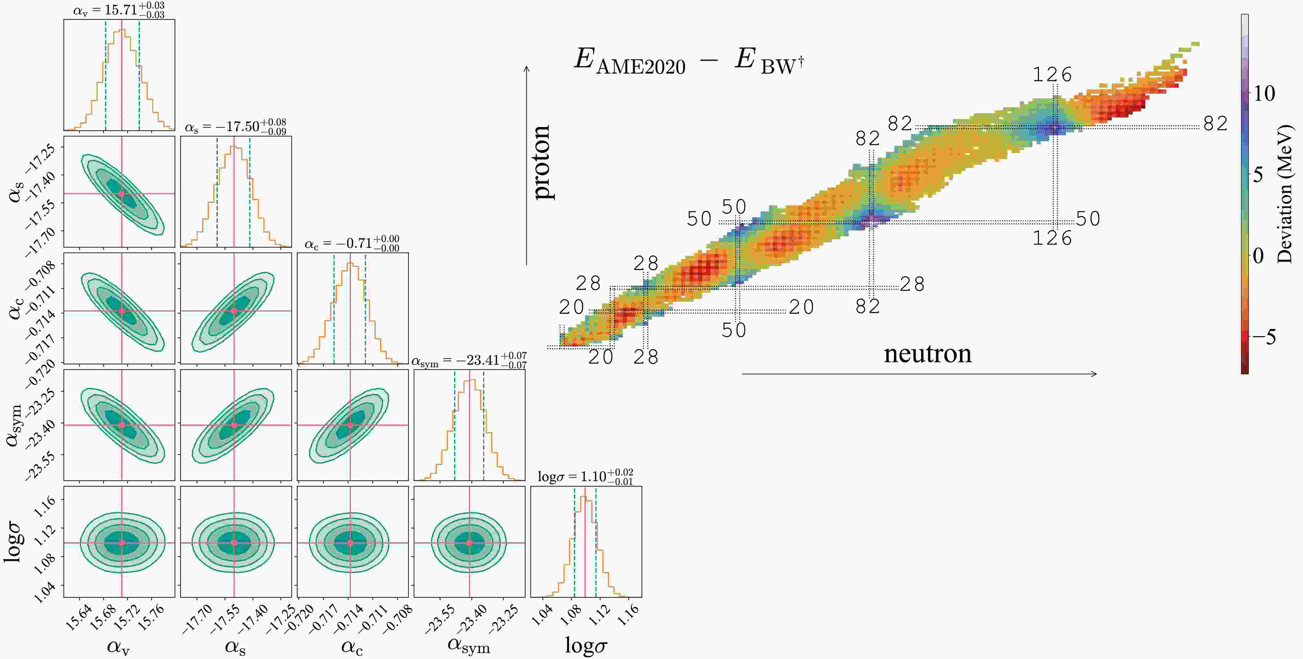
With the large data set of 2242 nuclei providing strong statistical constraints, the marginal posteriors of the BW* model are naturally highly symmetric (diagonal Gaussian-shaped plots in Fig. 1). The posterior distributions for all parameters of the BW* model exhibit symmetric, unimodal Gaussian shapes, with the posterior means concentrated within narrow ranges. This symmetric parameter space is mainly due to (i) the linear correlations among the four parameters ($ \alpha_\mathrm{v} $, $ \alpha_\mathrm{s} $, $ \alpha_\mathrm{c} $, $ \alpha_{\rm{sym}} $) of the BW* mass model [65, 76], which render the likelihood function equivalent to that of a multivariate linear regression; (ii) the adoption of Gaussian priors combined with a Gaussian likelihood, which mathematically yields a multivariate Gaussian joint posterior distribution [100]; and (iii) the absence of strong nonlinear terms or stringent physical constraints. The two-dimensional contour plots in Fig. 1 further reveal inverse correlations between $ \alpha_\mathrm{v} $ and $ \alpha_\mathrm{s} $, between $ \alpha_\mathrm{v} $ and $ \alpha_\mathrm{c} $, and between $ \alpha_\mathrm{v} $ and $ \alpha_{\rm{sym}} $, while $ \alpha_\mathrm{s} $, $ \alpha_\mathrm{c} $, and $ \alpha_{\rm{sym}} $ are positively correlated with one another.

Figure 1.  (color online) Posterior distributions of the four parameters of the BW* nuclear mass model. The two-dimensional (2D) contour levels indicate the 38%, 68%, 87%, and 95% credible regions. The one-dimensional (1D) marginalized posteriors are plotted along the diagonal, with the 68% credible interval shaded. The maximum-likelihood estimates for the 1D posterior of each parameter are reported above the corresponding subplot. The most probable distribution of each BW* parameter is shown at the top of the corresponding diagonal plot. The mean values of the posterior distributions of all four parameters of BW*, together with the corresponding physical units, are listed in the third column of Table 3. The optimal parameter set, together with the corresponding physical units, is presented in the fourth column of Table 3. The deviation between the BW^† and AME2020 binding energies is shown on the nuclear chart with respect to the color scale on the right.

The detailed correlation strengths among the model parameters are presented in the Pearson and Spearman rank correlation matrices in Table 6. As an example, the Spearman correlation coefficient for $ \alpha_\mathrm{v} $-$ \alpha_\mathrm{s} $ corresponds to $ \rho_{ij} $ in Eq. (23) with $ \theta_i=\alpha_\mathrm{v} $ and $ \theta_j=\alpha_\mathrm{s} $, i.e., $ \rho(\alpha_\mathrm{v},\alpha_\mathrm{s}) = -0.994 $. The Pearson coefficients are defined analogously, with $ r(\alpha_\mathrm{v},\alpha_\mathrm{s}) $ denoting $ r_{ij} $ for the same pair of posterior parameters in Eq. (25). Both the Spearman and Pearson correlation matrices are symmetric. The Spearman coefficients $ \rho_{ij} \gt 0 $ and $ \rho_{ij} \lt 0 $ indicate positive and negative correlations among the posterior parameters, respectively. These correlation patterns are consistent with the physical expectations of the model (Fig. 1). Furthermore, the joint distributions of σ with each parameter appear approximately circular, suggesting uniformly weak correlations.

Table 7 summarizes the effective sample size, $ n_\mathrm{eff} $, and Gelman–Rubin statistic, $ \hat{R} $, for all parameters of the BWK* mass model. All $ \hat{R} $ values below 1.04 indicate convergence of the Markov chains. The notably large value $ \hat{R}=1.1926 $ for $ \alpha_\mathrm{r} $ reveals a local Markov chain mixing bottleneck, indicating a statistical signature of parameter degeneracies and absorption of strength by other parameters. All $ n_\mathrm{eff} $ values exceed 2500, ensuring reliable posterior estimates. The posterior mean of the noise standard deviation σ is 1.601 MeV, with a $ 95\; $% credible interval of [1.55, 1.65] MeV.

The posterior distributions of the BWK* model show that several parameters deviate noticeably from Gaussian forms (diagonal plots in Fig. 2), exhibiting mild skewness and heavier tails that are not found in the BW* model. This reflects the nonlinearity introduced by the additional terms in the BWK* model and increases the complexity of the posterior landscape, which could not be captured by least-squares fitting methods. Moreover, Table 8, which presents the Pearson correlation and Spearman rank correlation matrices of the BWK* model, also reveals nonlinear but monotonic correlations among several key parameters, e.g., $ \rho(\alpha_\mathrm{sym},\alpha_\mathrm{st}) = -0.886 $, $ \rho(\alpha_\mathrm{w},\alpha_\mathrm{st}) = -0.632 $, and $ \rho(\alpha_\mathrm{m},\beta_\mathrm{m}) = -0.913 $. Positive correlations are also observed, e.g., $ \rho(\alpha_\mathrm{sym},\alpha_\mathrm{w}) = 0.660 $. These results agree with the finding of [14] that interplay and compensatory effects among different terms are important features of the semi-empirical mass formula.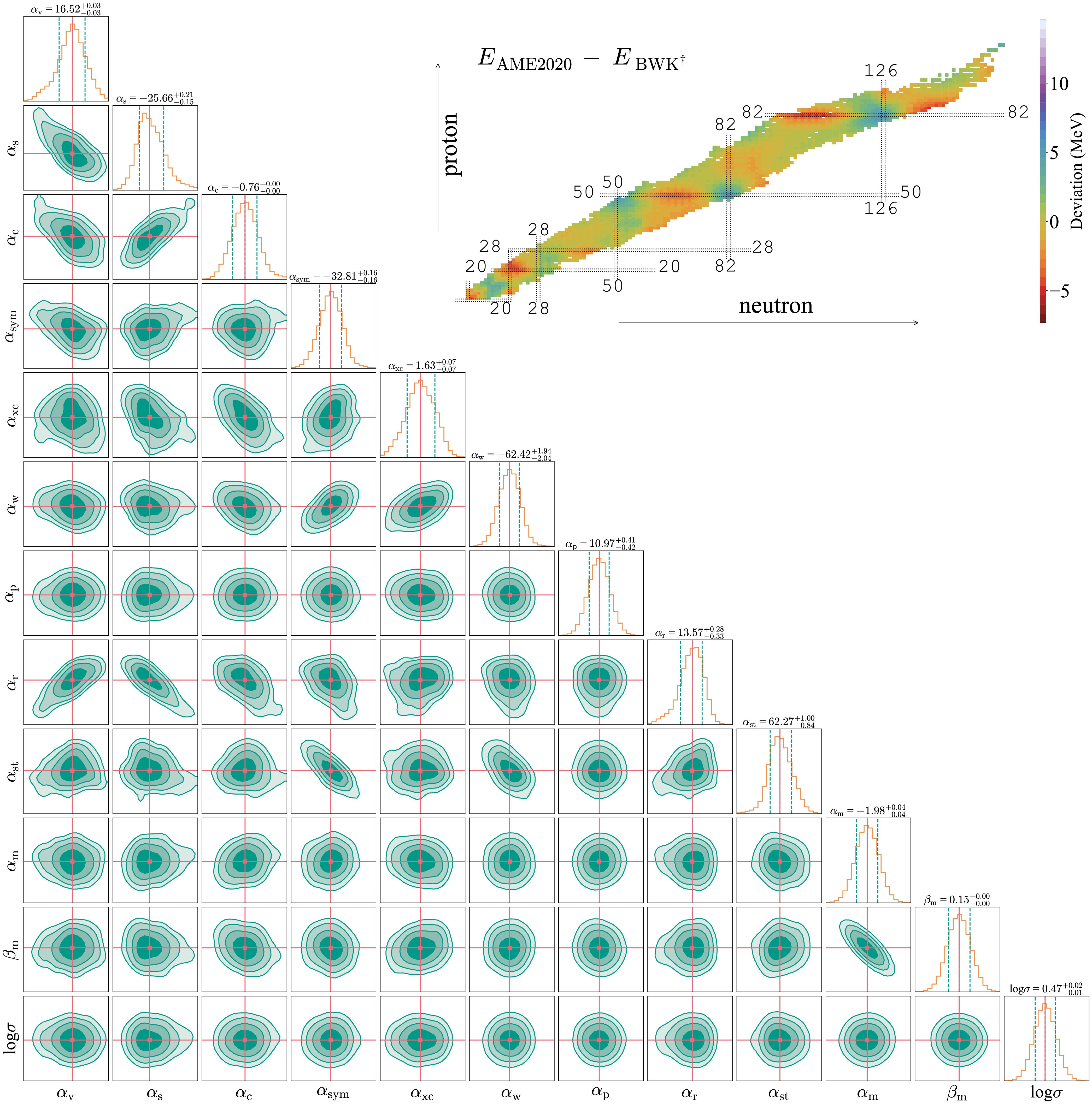

Figure 2.  (color online) Posterior distributions for all 11 parameters of the BWK* nuclear mass model. The most probable values of the BWK* parameters are shown at the top of the corresponding diagonal plots. The mean values of the posterior distributions for all 11 parameters, together with the corresponding physical units of BWK*, are listed in the sixth column of Table 3. The optimal parameter set is presented in the seventh column of Table 3. The deviations between the BWK^† and AME2020 binding energies are presented on the nuclear chart with respect to the color scale on the right. See Fig. 1 for the remainder of the description.

The analysis of the posterior distributions reveals mild multimodality in several BWN* parameters, namely $ \alpha_\mathrm{v} $, $ \alpha_\mathrm{s} $, $ \alpha_\mathrm{c} $, and $ \alpha_\mathrm{r} $ (diagonal plots in Fig. 3). Table 9 shows that the Gelman–Rubin statistics $ \hat{R} $ for all parameters remain below 1.04 and that $ n_\mathrm{eff} $ exceeds 2500 for every parameter, indicating that the multi-chain MCMC sampling for the BWN* model has achieved excellent convergence. This multimodality is not a sampling artifact; rather, it reflects the structures arising from the shell-correction and pairing terms introduced in the BWN* model (Eq. (3)).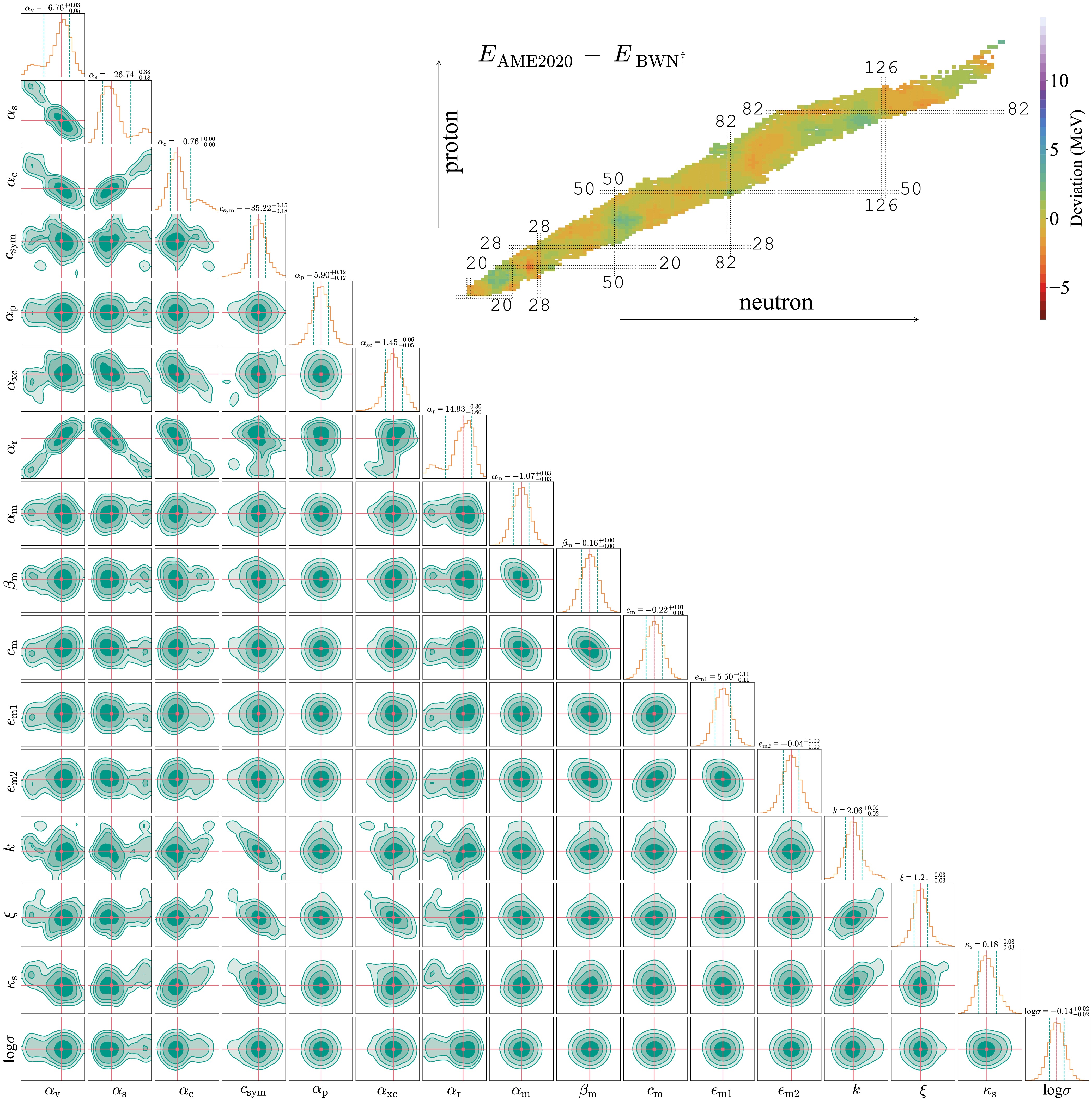

Figure 3.  (color online) Posterior distributions for all 15 parameters of the BWN* nuclear mass model. The most probable value of each BWN* parameter is shown at the top of the corresponding diagonal plot. The mean values of the posterior distributions for all 15 parameters, along with the corresponding physical units of BWN*, are listed in the third column of Table 4. The optimal parameter set is presented in the fourth column of Table 4. The deviation between the BWN^† and AME2020 binding energies is presented on the nuclear chart with respect to the color scale on the right. See Fig. 1 for the remainder of the description.

The main asymmetric correlations of $ \alpha_\mathrm{sym} $-$ \alpha_\mathrm{st} $, $ \alpha_\mathrm{w} $-$ \alpha_\mathrm{st} $, $ \alpha_\mathrm{m} $-$ \beta_\mathrm{m} $, and $ \alpha_\mathrm{sym} $-$ \alpha_\mathrm{w} $ in the BWK* model are inherited by the BWN* model. The detailed correlation strengths among the model parameters are presented in Table 10. In the BWN* model, the symmetry energy term $ \alpha_{\rm{sym}} $ and the related Wigner and surface-symmetry correction terms in the BWK model are combined into a single term with the redefined $ \alpha_{\rm{sym}} $, consisting of $ c_{\rm{sym}} $, k, and ξ, together with the surface diffuseness factor $ f_s $ calibrated by $ \kappa_\mathrm{s} $. The original BW correlation in the symmetry term has thus been restructured into a set of separable nonlinear terms, i.e., (i) the $ k/A^{1/3} $ term, which accounts for the reduction in symmetry energy due to surface effects; (ii) the ξ term, which provides ad hoc corrections for nuclei with extreme isospin asymmetry; and (iii) the $ f_\mathrm{s} $ factor, which introduces the contribution of surface diffuseness and is implicitly correlated with nuclear surface properties. The former two separable terms fine-tune the BWN model to better reproduce experimental binding energies in regions far from the β-stability line than the previous linear form does.

According to the Spearman rank correlation matrix in Table 10, the parameters of the new terms in the BWN* model show nonlinear yet monotonic correlations, i.e., $ \rho(c_{\rm{sym}},\xi) = -0.556 $, $ \rho(c_{\rm{sym}},k) = -0.881 $, $ \rho(c_{\rm{sym}},\kappa_\mathrm{s}) = -0.524 $,$ \rho(k,\xi) = 0.520 $, and $ \rho(k,\kappa_\mathrm{s}) = 0.685 $. Meanwhile, the posterior distributions in the BWN* model exhibit multimodality (diagonal plots of $ \alpha_\mathrm{v} $, $ \alpha_\mathrm{s} $, $ \alpha_\mathrm{c} $, and $ \alpha_\mathrm{r} $ in Fig. 3) and parameter degeneracies (e.g., covariance plots of $ \alpha_\mathrm{v} $-$ c_{\rm{sym}} $, $ c_{\rm{sym}} $-$ \alpha_\mathrm{r} $, $ \alpha_\mathrm{v} $-k, and $ \alpha_\mathrm{xc} $-k in Fig. 3).

By using the condition number of the Pearson correlation matrix to analyze parameter degeneracy in the BWN* model, we obtain $ {\cal{K}}({\boldsymbol{R}}_\mathrm{P}) = 1.42 \times 10^6 $, indicating strong linear degeneracy. However, this result contradicts the covariance plots in Fig. 3. For the BWN* model, the condition number of the Spearman rank correlation matrix is $ {\cal{K}}({\boldsymbol{R}}_\mathrm{S}) = 8.14 \times 10^2 \lt 10^3 $ (Eq. (24)), which implies that the degeneracy is rather weak, consistent with the overall covariance plots in Fig. 3. The compensation effects could originate from nonlinear parameter manifolds rather than from linear degeneracy. The weak parameter degeneracies could be alleviated by introducing new terms or deformation corrections to reshape the posterior parameter space. In this work, we take into account deformation corrections (Sec. III.D) to alleviate the parameter degeneracies, whereas the introduction of new term(s) is left for future work and is beyond the scope of this study.

The corner plots in Fig. 3 reveal negative correlations among $ c_\mathrm{m} $, $ \alpha_\mathrm{m} $, and $ \beta_\mathrm{m} $. The corresponding elements of the Spearman rank correlation matrix for $ c_\mathrm{m} $-$ \alpha_\mathrm{m} $, $ c_\mathrm{m} $-$ \beta_\mathrm{m} $, and $ \alpha_\mathrm{m} $-$ \beta_\mathrm{m} $ in Table 10 provide the numerical details of these negative correlations. The $ c_\mathrm{m}(v_\mathrm{n} + v_\mathrm{p})$ term is a linear correction with $ c_\mathrm{m} = -0.22\pm0.01$ (posterior plot of $ c_\mathrm{m} $ in Fig. 3), which decreases the influence incurred from the shell effect as the total valence number increases away from magic numbers. In regions of large valence numbers, this linear term is interrelated with $ \alpha_\mathrm{m} P$, such that when the $ c_\mathrm{m}(v_\mathrm{n} + v_\mathrm{p})$ term becomes more negative, $ \alpha_\mathrm{m} P$ tends to maintain the overall shell-correction energy. Similarly, $ c_\mathrm{m}$ is interrelated with $ \beta_\mathrm{m}$ because the cumulative effect of the $ c_\mathrm{m}(v_\mathrm{n} + v_\mathrm{p})$ term partially absorbs the influence of the quadratic $ \beta_\mathrm{m} P^2$ term in regions between magic numbers.

In addition, a weak positive correlation is observed between $ c_\mathrm{m}$ and $ e_\mathrm{m2}$. The exponential term $ e_\mathrm{m1} \delta_{\rm{shell}} \exp(e_\mathrm{m2} (v_\mathrm{p}^2 + v_\mathrm{n}^2))$, with $ e_\mathrm{m2} \lt 0$, provides strongly enhanced (quenched) shell correction near (away from) magic numbers. A mutual balance is established between the exponential term and the linear $ c_\mathrm{m}(v_\mathrm{n} + v_\mathrm{p})$ term, in which the exponential term dominates the enhancement near closed shells, while the linear term smoothly quenches the correction for large valence numbers. For instance, in regions near magic numbers, when $ e_\mathrm{m2}$ is less negative and $ c_\mathrm{m}$ is therefore also required to be less negative, the shell effect is strengthened, demonstrating the compensatory nature of the two terms. The BA-MCMC analysis naturally indicates this behavior, consistent with the least-squares fitting results presented in Ref. [17]. See Table 4 for ($ e_\mathrm{m2} = -0.0444$, $ c_\mathrm{m} = -0.2343$) of BWN obtained from the least-squares fit and ($ e_\mathrm{m2} = -0.0420$, $ c_\mathrm{m} = -0.2243$) of BWN* generated from BA-MCMC.

Table 11 presents the effective sample size, $ n_\mathrm{eff} $, and the Gelman-Rubin statistic, $ \hat{R} $, for all parameters of the BWL* mass model. It also provides the posterior convergence diagnostics for the reference chain of the BWL* model. Most parameters exhibit excellent convergence, with the potential scale reduction factor $ \hat{R} $ close to 1.00 and the effective sample size $ n_\mathrm{eff} $ comfortably exceeding 2500. In particular, the newly introduced deformation-correction parameters, $ g_1, g_2 $, and γ, display high sampling efficiency ($ \hat{R} \leqslant 1.0034 $), demonstrating that the incorporation of deformation correction successfully regularizes the complex posterior landscape and resolves the parameter degeneracy observed in BWN*. A minor statistical exception is observed for ξ, with $ \hat{R} = 1.1757 $, indicating slow convergence across multiple Markov chains. Overall, the diagnostics confirm that the parameter space of the BWL* model is well converged and robust for posterior inference, despite the slow convergence across multiple chains.

Basically, the BWL* model preserves the positively and negatively correlated parameters and the major contributing terms of the BWK* and BWN* models. The detailed correlation strengths among the parameters of the BWL* model are presented as Pearson correlation and nonlinear Spearman rank-correlation matrices in Table 12.

After incorporating the deformation corrections (Eq. (5)), the condition number of the Pearson correlation matrix decreases from $ 1.42 \times 10^6 $ for BWN* to $ 1.13 \times 10^6 $ for BWL*, demonstrating a moderate reduction in parameter degeneracy. Importantly, the condition number of the nonlinear Spearman rank-correlation matrix for BWL* increases to $ 1.09 \times 10^3 $, compared with $ 8.14 \times 10^2 $ for BWN*. This suggests that the BA-MCMC and Spearman rank-correlation analysis method permits the reduction of parameter collinearity in both models to be revealed. This outcome is consistent with the introduction of additional nonlinear terms into the mass models and highlights the limitation of evaluating a mass model using a least-squares fit and a Pearson correlation matrix.

By incorporating the deformation-correction terms with the parameters $ g_1 $, $ g_2 $, and γ (Eq. (5)), the BWL* model alleviates the multimodality observed in several posterior distributions of the BWN* model. This improvement is indicated by comparison of the diagonal plots of $ \alpha_\mathrm{v} $, $ \alpha_\mathrm{s} $, $ \alpha_\mathrm{c} $, and $ \alpha_\mathrm{r} $ in Figs. 3 and 4. The consideration of deformation smooths the likelihood surface, making the posterior distributions more unimodal (e.g., the covariance plots of $ \alpha_\mathrm{v} $, $ \alpha_\mathrm{s} $, $ \alpha_\mathrm{c} $, and $ \alpha_\mathrm{r} $ in Fig. 4).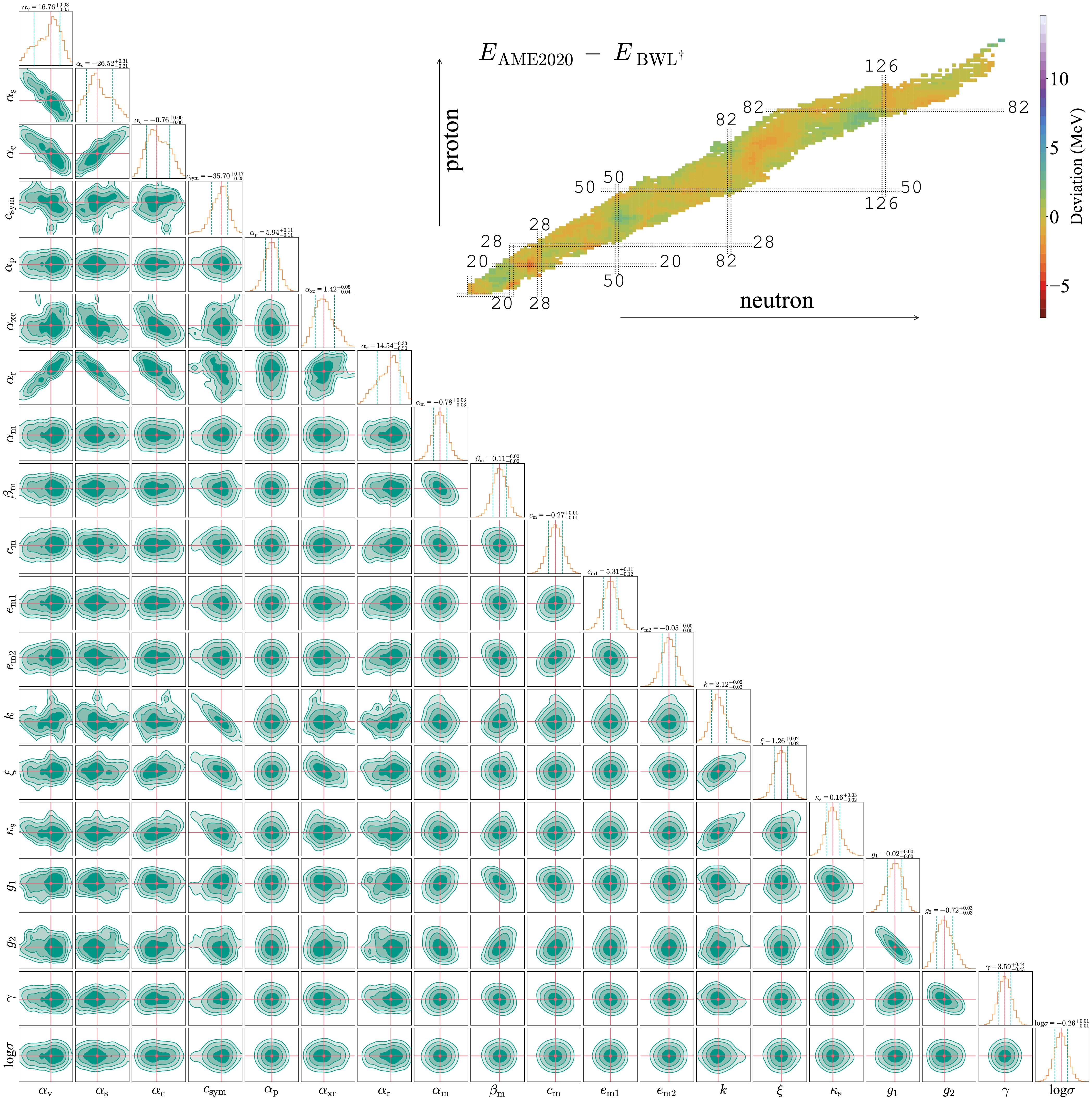

Figure 4.  (color online) Posterior distributions of all 18 parameters of the BWL* nuclear mass model. The most probable value of each BWL* parameter is shown at the top of the corresponding diagonal plot. The mean values of the posterior distributions of all 18 parameters, along with the corresponding physical units of BWN*, are listed in the fifth column of Table 4. The optimal parameter set is presented in the sixth column of Table 4. The deviation between the BWL^† and AME2020 binding energies is presented on the nuclear chart with respect to the color scale on the right. See Fig. 1 for the remainder of the description.

The posterior distributions of the BWL* model reveal new nonlinear yet monotonic correlations among the parameters $ g_1 $, $ g_2 $, and γ (Eq. (7)). In Table 12, the compensation between the deformation correction coefficients $ g_1 $ and $ g_2 $ is indicated by $ \rho(g_1,g_2)=-0.926 $. These two parameters calibrate the deformation correction factor (Eq. (6)) such that $ g_1 $ strengthens the first-term deformation correction, whereas $ g_2 $ weakens the second-term correction, thereby smoothing the overall deformation correction strength applied to the macroscopic energy.

The Spearman rank correlation coefficients $ \rho(g_1,\gamma) $ and $ \rho(g_2,\gamma) $ are 0.285 and $ -0.546 $, respectively. The positive (negative) value of $ \rho(g_1,\gamma) $ ($ \rho(g_2,\gamma) $) indicates that γ is positively (negatively) correlated with $ g_1 $ ($ g_2 $). See Eqs. (6) and (9) for details. These factors, $ g_1 $, $ g_2 $, and γ, are optimized through BA-MCMC to describe the total binding energy of strongly deformed nuclei. The Spearman rank correlation coefficient $ \rho(\beta_\mathrm{m},g_2)=0.515 $ quantifies the positive correlation between the quadratic shell correction and the second term of the deformation correction in Eq. (7). The Spearman rank correlation coefficients $ \rho(\alpha_\mathrm{m},g_1)=0.296 $ and $ \rho(\alpha_\mathrm{m},g_2)=-0.339 $ suggest a positive correlation between $ \alpha_\mathrm{m} $ and $ g_1 $ and a negative correlation between $ \alpha_\mathrm{m} $ and $ g_2 $, respectively.

Here, we discuss several cases to illustrate the correlations among $ g_1 $, $ g_2 $, γ, and $ \alpha_\mathrm{m} $. A first-order expansion of the macroscopic deformation factor in Eq. (6), after substituting Eq. (7), gives the deformation contributions proportional to $ g_1 $ and $ g_2 $,

of which the non-leading-order terms are negligible. For nuclei with $ |\beta_2| \lt 0.01 $ and $ P = {\nu_\mathrm{p} \nu_\mathrm{n}}/({\nu_\mathrm{p} + \nu_\mathrm{n}}) = 0 $, the total contribution of $ \Delta B_{g_1}^{(1)} $ and $ \Delta B_{g_2}^{(1)} $ is smaller than $ 0.01 $ MeV. For instance, for $ ^{90} $Zr, $ \Delta B_{g_1}^{(1)} $ and $ \Delta B_{g_2}^{(1)} $ are 0.004 MeV and $ -0.006 $ MeV, respectively; for $ ^{208} $Pb, they are $ +0.003 $ MeV and $ -0.004 $ MeV, respectively. The macroscopic energies of $ ^{90} $Zr and $ ^{208} $Pb are quenched by the deformation parameter $ |\beta_2| $ through the deformation correction, and $ B_i^{\text{shell}} $, consisting of the deformation quenching factor (Eq. (9)) and shell correction (Eq. (10)), dominates their binding energies.

For $ ^{238} {\rm{U}}$, $ ^{240} {\rm{Pu}}$, and $ ^{244} {\rm{Cm}}$, the corresponding $ \beta_2 $ values are 0.2155, 0.2213, and 0.2261, respectively [86]. Meanwhile, the corresponding $ \Delta B_{g_1}^{(1)} $ and $ \Delta B_{g_2}^{(1)} $ values for $ ^{238} {\rm{U}}$, $ ^{240} {\rm{Pu}}$, and $ ^{244} {\rm{Cm}}$, in units of MeV, are 14.056 and $ -13.171 $, 14.439 and $ -13.128 $, and 14.394 and $ -12.352 $, respectively. These $ \Delta B_{g_1}^{(1)} $ and $ \Delta B_{g_2}^{(1)} $ terms, associated with $ g_1 $ and $ g_2 $, form a counterbalancing relationship and therefore nearly cancel each other in their contribution to the macroscopic LDM energy. Following the complete product in Eq. (6), the net macroscopic deformation corrections for $ ^{238} {\rm{U}}$, $ ^{240} {\rm{Pu}}$, and $ ^{244} {\rm{Cm}}$ are $ +0.883 $, $ +1.310 $, and $ +2.041 $ MeV, respectively. The suppressive role of the deformation quenching factor (Eq. (9)) is important for calibrating the dominant $ \alpha_\mathrm{m}P $ term in its contribution to the bound energy through $ B_i^{\text{shell}} $ for $ ^{238} {\rm{U}}$, $ ^{240} {\rm{Pu}}$, and $ ^{244} {\rm{Cm}}$. The quenched $ B_i^{\text{shell}} $ values in the BWL^† model for $ ^{238} {\rm{U}}$, $ ^{240} {\rm{Pu}}$, and $ ^{244} {\rm{Cm}}$ are $ -4.498 $, $ -5.031 $, and $ -5.730 $ MeV, respectively. By combining the effects of the deformation correction factor (Eq. (6)) and deformation quenching factor (Eq. (9)), the residuals of $ ^{238} {\rm{U}}$, $ ^{240} {\rm{Pu}}$, and $ ^{244} {\rm{Cm}}$ in BWL^† are reduced from $ +0.641 $ to $ +0.058 $ MeV, from $ +0.776 $ to $ +0.141 $ MeV, and from $ +0.795 $ to $ +0.065 $ MeV, respectively, compared with those in BWN^†.

Collectively, these correlations demonstrate that the deformation correction terms ($ g_1 $, $ g_2 $, γ) and the shell correction terms ($ \alpha_\mathrm{m} $, $ \beta_\mathrm{m} $) in the BWL* model exhibit significant physical compensation relationships. In addition, the introduction of the deformation parameters $ g_1 $, $ g_2 $, and γ regularizes the overall posterior distribution, making it more symmetric and reducing parameter degeneracy in BWK* and BWN*.

The compensation relationships between k-ξ, k-$ \kappa_\mathrm{s} $, and ξ-$ \kappa_\mathrm{s} $ become more pronounced in the covariance plots of the BWL* model (Fig. 4). This indicates that the inclusion of deformation corrections leads to a set of less degenerate posterior distributions. Consequently, the four parameters $ c_{\rm{sym}} $, k, ξ, and $ \kappa_\mathrm{s} $ support the synergy of the isospin-dependent symmetry energy terms from the WS4 model in the BWN* formulation by Wu et al. (2025).

By comparing the mean difference in Z between the BWN^† and BWL^† models, it is evident that introducing the macro deformation correction factor (Eq. (6)) noticeably reduces the overall residuals between the theoretical and AME2020 mass values for nuclei with $ Z \gt 82 $ (Fig. 5). The most pronounced improvement is observed in the actinide region, $ Z= $89–103. The mean absolute residual error (MAE) decreases from $ 0.7517 $ to $ 0.3566 $ MeV, corresponding to a reduction of approximately 53 %. Nuclei in this open-shell actinide region are generally well deformed, and their equilibrium shapes reflect the interplay between macroscopic deformation energy and shell corrections [101−103]. In the light-nucleus region, $ Z \lt 20 $, the MAE decreases from $ 1.0653 $ to $ 0.8710 $ MeV, corresponding to a reduction of $ \approx 18\; $%, particularly for nuclei with $ Z \lt 15 $. Moreover, near the proton magic number $ Z = 50 $, the residual of BWL^† is up to 713 keV lower than that of BWN^†. This demonstrates that the deformation quenching factor (Eq. (9)) suppresses shell effects in both single-magic and open-shell nuclei. In fact, this improvement also benefits from the more comprehensive characterization of shell effects achieved by the BWN^† model.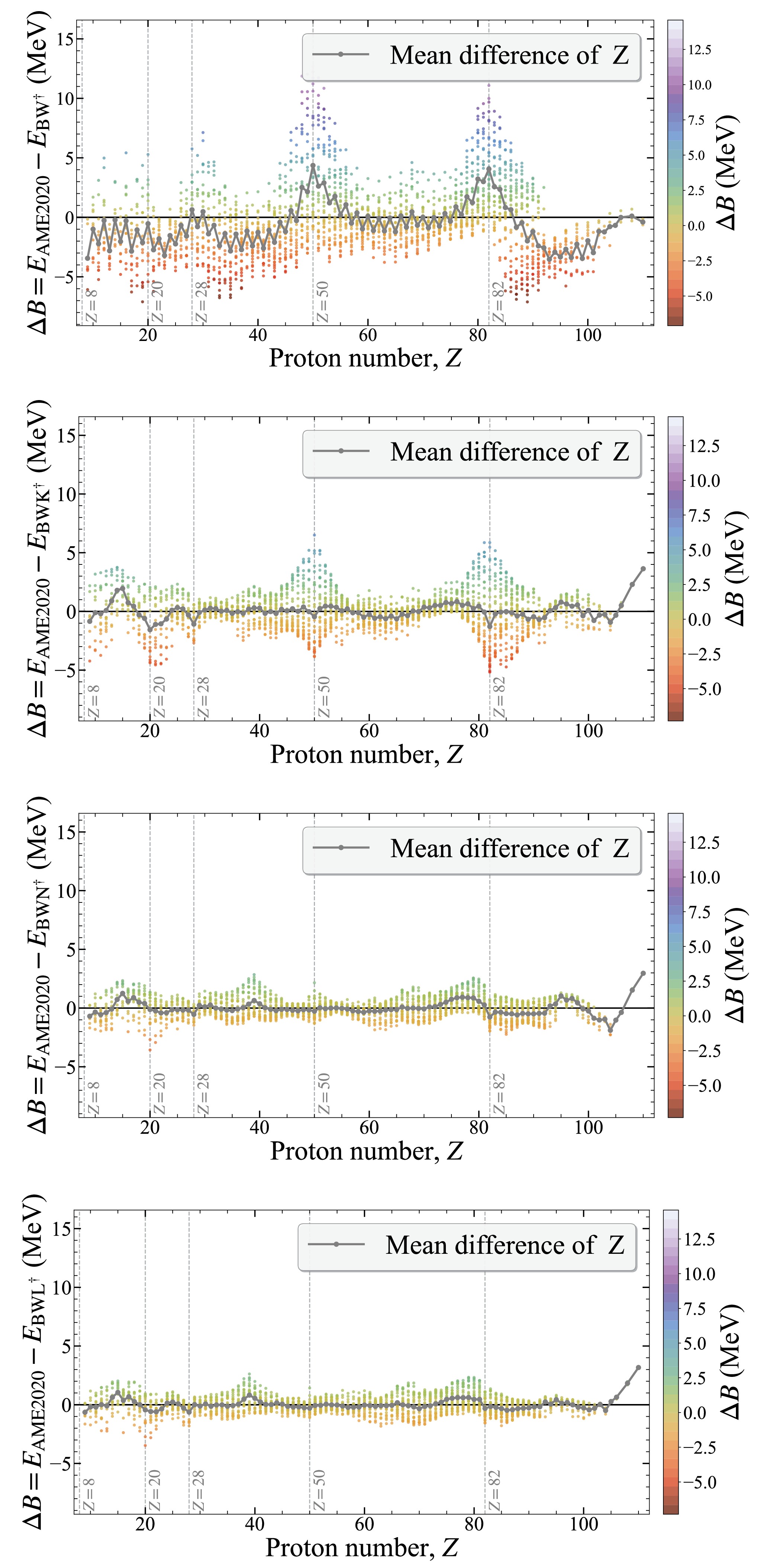

Figure 5.  (color online) Deviations in nuclear binding energies between AME2020 and BW^†, BWK^†, BWN^†, and BWL^†.

The BWL^† model reduces the global RMS deviation of the BWN^† model from 0.863 to 0.759 MeV for the 2242 selected nuclei, corresponding to an improvement of approximately 12%. As shown in Fig. 6, among the mass models, BWL^† yields the lowest average residuals in the light-nuclei region with $ Z<20 $. However, the residuals of individual nuclides are still not significantly reduced, suggesting that the descriptive capability of the deformation corrections in BWL^† may have been exhausted, whereas the shell correction terms can still be improved.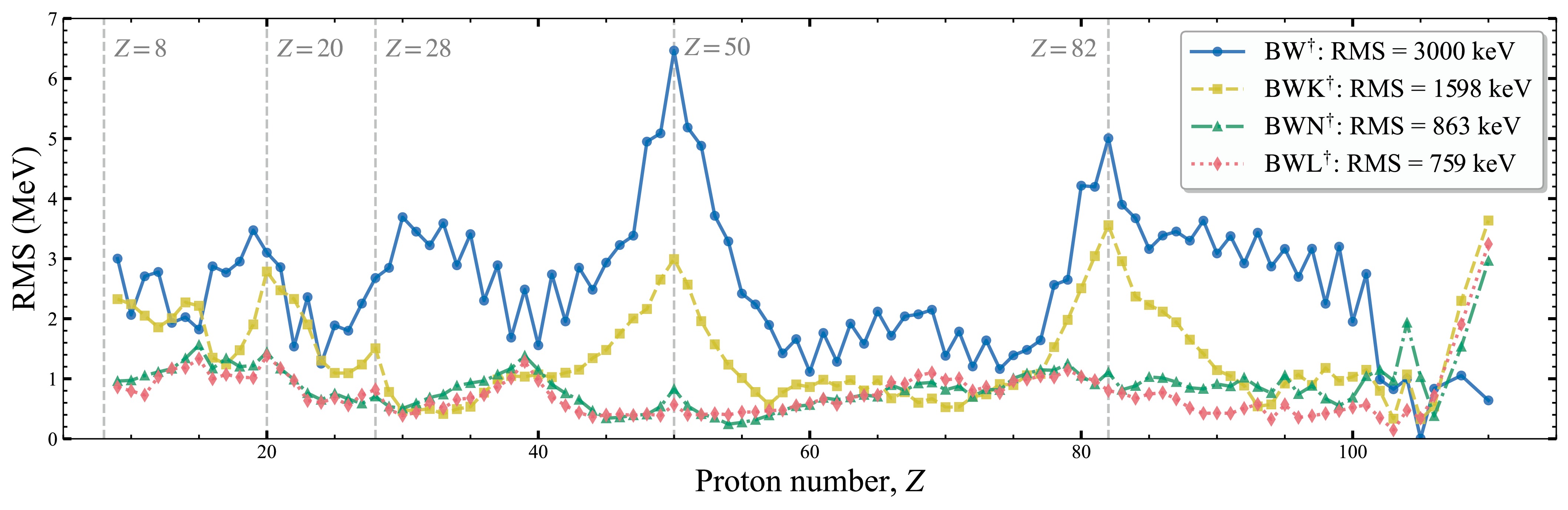

Figure 6.  (color online) Root-mean-square deviations (RMSs) between the experimental and theoretical binding energies from BW^†, BWK^†, BWN^†, and BWL^† for each isotopic chain. See Tables 3 and 4 for the BA-MCMC-optimized mass models.

For the medium-heavy mass region of $ Z\approx $28−50, the BWL^† model produces the lowest overall RMS among all mass models. Nevertheless, deformation is weak in the region around $ Z=40 $; for example, the average quadrupole deformation is $ \overline{\beta_2}=0.0962$ for yttrium isotopes ($ Z=39 $), whereas shell effects dominate and cause these isotopes to become more overbound than their experimental counterparts. For the rare-earth region, the mean residuals (Fig. 5) and RMS values (Fig. 6) also demonstrate that the shell correction term (Eq. (10)) can be further improved.

For the actinide and superheavy region with $ Z>82 $, especially near $ Z \approx 100 $, the mean residuals and RMS values of BWL^† remain superior to those of the other models. Improved predictions of unmeasured masses are of considerable importance for estimating fission behavior and the synthesis of superheavy nuclei [104, 105].

For the historically large discrepancies along the isotopic chains of the magic proton numbers $ Z=50 $ and 82, the RMS values of these chains are successively reduced through refinements and BA-MCMC optimization of these models. Both BWN^† and BWL^† reasonably reproduce the experimental data. The difference in RMS between these two models is at most 308 keV, indicating that the spherical shell effect inherited from BWN^† by BWL^† helps reproduce the experimental data.

We plot the RMS deviation as a function of the WS4 quadrupole deformation parameter $ \beta_2 $ in Fig. 7 to quantify the deformation dependence of the BWN^† and BWL^† models. As indicated by the 14 nonzero points at $ \beta_2\lessapprox0.25 $, BWL^† yields lower RMS values than BWN^†, with a count-weighted average RMS reduction of about $ 0.105 $ MeV. The reduction is about $ 0.09 $–$ 0.13 $ MeV in the region $ \beta_2\approx0.10 $–$ 0.24 $, where many deformed nuclei are located. In the two largest $ \beta_2 $ bins, containing 73 and 23 nuclei, the RMS values are nearly identical, with differences of 0.24−5 keV. This analysis indicates that the inclusion of deformation-dependent terms in BWL improves the mass description over a broad range of deformed nuclei, rather than merely through a global refit of parameters.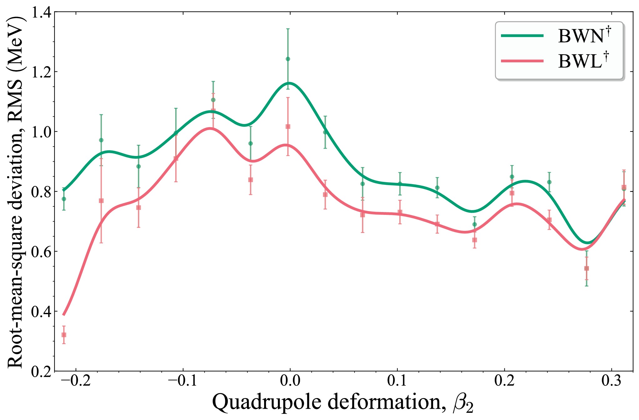

Figure 7.  (color online) RMS deviation as a function of the quadrupole deformation parameter $ \beta_2 $. Both BWL^† (red line) and BWN^† (blue line) are plotted using equal-width bins over the interval $ -0.2635\leq\beta_2\leq0.3289 $, with bin width $ \Delta\beta_2\approx $$ 0.035 $. Because deformation is not included in BWN^†, the RMS deviations of BWN^† are plotted only for comparison, using the same interval as for the nuclei in BWL^†. Bins containing fewer than 8 nuclei are discarded, leaving 16 effective points, as shown.

BA-MCMC provides full posterior distributions for all model parameters. These posterior distributions naturally incorporate physically motivated priors and jointly infer the noise level [65]. By contrast, the least-squares fitting method can provide only point estimates and asymptotic errors. This advantage of BA-MCMC enables direct analysis of the joint distributions and strong correlations among parameters from the posterior distribution plots, thereby providing statistical evidence (a reliable basis) for further physical simplification of the model.

For instance, the posterior distributions of the BW* model exhibit more symmetric shapes than the overall distributions of the BWK* model, which show some breakdown of symmetry (Figs. 1 and 2). The posterior distributions of individual parameters in the BWK* model deviate slightly from Gaussian shapes and exhibit skewness with longer tails, causing the overall joint posterior distributions to depart from an elliptical shape. The underlying reason is that the introduction of Coulomb exchange, Wigner, pairing, and surface-symmetry energies, together with the implementation of physical boundary constraints on the BWK* parameters (e.g., $ \beta_\mathrm{m} \gt 0 $), when combined with Gaussian priors, produces non-Gaussian posteriors [76]. Although the posterior distributions of the BWK* model are asymmetric, the BWK* model provides a substantially more comprehensive foundation for the subsequent development of the BWN* and BWL* models.

Further posterior analysis of the BWK model reveals that the Wigner term is positively correlated with the symmetry energy term (the posterior plot of $ \alpha_\mathrm{sym} $-$ \alpha_\mathrm{w} $ in Fig. 2, with the Spearman rank correlation coefficient $ \rho(\alpha_\mathrm{sym},\alpha_\mathrm{w})=0.660 $ in Table 8), while both the symmetry energy term and the Wigner term exhibit negative correlations with the surface-symmetry term (the posterior plots of $ \alpha_\mathrm{sym} $-$ \alpha_\mathrm{st} $ and $ \alpha_\mathrm{w} $-$ \alpha_\mathrm{st} $ in Fig. 2, with the Spearman rank correlation coefficients $ \rho(\alpha_\mathrm{sym},\alpha_\mathrm{st})=-0.886 $ and $ \rho(\alpha_\mathrm{w},\alpha_\mathrm{st})=-0.632 $ in Table 8). The posterior plots of these terms show pronounced correlations, indicating highly similar physical meanings and compensatory effects, which underpins the merging of these highly correlated terms in the development of the BWN model. This, in turn, enables the construction of a more concise nuclear mass model while preserving the essential physical meaning. BA-MCMC not only validates the rationale for this combination but also quantifies the uncertainty of the merged parameters through the full posterior distributions, thereby providing important theoretical guidance and statistical support for the future development of new optimized macroscopic-microscopic nuclear mass models.

The posterior structure of the parameter space of the BWN* model (Fig. 3) is significantly altered in the BWL* model (Fig. 4) by the introduction of a deformation correction factor in the macroscopic part and a deformation quenching factor in the shell correction term (Eq. (5)) [18, 19, 29]. The multimodality observed in several BWN* parameters (i.e., $ \alpha_\mathrm{v} $, $ \alpha_\mathrm{s} $, $ \alpha_\mathrm{c} $, $ \alpha_\mathrm{r} $, and $ \alpha_\mathrm{r} $) is alleviated in the BWL* model. The general posterior distributions become more unimodal, symmetric, and smooth. Analysis of the posterior distributions of the BWN* and BWL* models reveals that the newly introduced deformation parameters $ g_1 $ and $ g_2 $ effectively smooth the likelihood surface, reduce parameter degeneracies, and regularize the joint posterior distributions.

To verify the generality of the deformation scheme (quadrupole and high-multipole deformation and quenched shell correction), we applied exactly the same deformation form to the BWK^† model. The inclusion of deformation further reduces the RMS deviation of the BWK^† model from 1.598 to 1.476 MeV, demonstrating the universality of this deformation scheme in phenomenological models. Moreover, by replacing AME2020 with the WS4 mass data [86] as the counterpart pseudo-data, we reoptimized BWL with BA-MCMC and obtained a set of BWL^‡ parameters (the seventh column of Table 4) with an RMS of $ 0.763 $ MeV. The difference between the BWL* and BWL^‡ parameters is at most 9.3%. In fact, the BWL^‡ parameters lie within the uncertainty range of BWL*, implying the universality of BA-MCMC in optimizing BWL to reproduce both AME2020 and WS4 masses, for which the RMS difference between the AME2020 and WS4 masses is 0.283 MeV [19].

Using the BA-MCMC method, the BWN model is optimized to produce an RMS of 863 keV. Meanwhile, the introduction of deformation correction terms into the BWN model reduces the RMS from 863 keV to 759 keV (Table 4), corresponding to an approximate RMS reduction of 12 %. Moreover, the MAE decreases by $ \approx 53 $ % in the actinide region ($ Z \gt 82 $) and by $ \approx 18 $ % in the light-nuclei region ($ Z \lt 20 $), while the average residual as a function of Z decreases noticeably. These results demonstrate that the implicit incorporation of deformation not only improves the posterior estimates of the parameters but also enhances the model's descriptive power in strongly deformed and light-mass regions, thereby providing a solid foundation for the future development of more refined macroscopic-microscopic nuclear mass models [106].

Nevertheless, all BW^†, BWK^†, and BWN^† mass models produce systematic deviations from AME2020 in the rare-earth region ($ A \approx 150 $−$ 190 $, $ Z \approx 60 $−$ 76 $), with local RMS values of 1.678 MeV, 0.720 MeV, and 0.814 MeV, respectively. Although the BWL^† model includes deformation, it produces a local RMS of 0.840 keV, which is slightly higher than that of BWN^† (Figs. 5 and 6). According to Möller et al. [103], 82.3 % ($ \beta_2 \gt 0.10 $) of nuclei in the rare-earth region exhibit prominent quadrupole deformation in the shape of a prolate ellipsoid [101]. The shell correction in the BWL^† model, which is dominated by the valence proton-neutron interaction factor, $ P ={\nu_\mathrm{p} \nu_\mathrm{n}}/(\nu_\mathrm{p} + \nu_\mathrm{n}) $, and the piecewise constant $ \delta_{\rm{shell}} $, even when damped by the deformation quenching factor $ \exp(-\gamma \displaystyle\sum\nolimits_k \beta_k^2) $, does not describe deformation-induced shell gaps well; these require a microscopic description of single-particle spectra [102]. Therefore, the remaining residuals in the rare-earth region should be attributed to the limitation of the present phenomenological shell correction rather than to the introduced deformation correction. As shown in Fig. 5, the BWL^† residuals still exhibit mean deviations similar to those of BWN^† in this region.

The posterior space in the BA-MCMC analysis increases as the number of physical terms and parameters grows from 5 (for the BW model) to 19 (for the BWL model). We observe that this high-dimensional posterior space causes slower chain mixing; consequently, the Gelman-Rubin $ \hat{R}$ values can exceed 1.1 for some parameters, resulting in non-Gaussian or multimodal posterior distributions. Therefore, longer MCMC chains (40 million steps per model in this work), much longer burn-in periods (the first 20 million samples used for exploring the parameter space must be discarded), and higher-resolution covariance adaptation must be implemented to generate reliable posteriors. As a result, the cost-effectiveness of MCMC exploration becomes strained. Under the same hardware configuration, the computational speed is reduced by more than 93% when comparing the analyses of the BW and BWL models. More advanced GPUs with adequate memory resources may help overcome such performance bottlenecks or delays.

In this work, we systematically investigated the Bethe-Weizsäcker variant nuclear mass models, i.e., BW, BWK, BWN, and BWL, using a full Bayesian analysis with Markov chain Monte Carlo sampling (BA-MCMC).

BA-MCMC reveals rich compensation (degeneracy) relations among the model parameters. For the BWK^† model, strong negative correlations are observed among the volume, surface, Coulomb, and curvature terms, as well as between the linear $ \alpha_\mathrm{m} $ and quadratic shell-correction coefficients $ \beta_\mathrm{m} $. The BWN^† model preserves most of the non-symmetric correlations after introducing the isospin-dependent symmetry energy, while new correlations emerge among the symmetry parameters $ c_{\rm{sym}}$, k, ξ, and $ \kappa_\mathrm{s}$. By implicitly incorporating deformation corrections, the BWL^† model reshapes the posterior parameter space and alleviates the multimodality and strong degeneracies observed in BWN^†, resulting in more unimodal and symmetric posterior distributions.

Quantitatively, the BWL model further improves upon the BWN model by introducing the deformation scheme, reducing the global RMS deviation for 2242 nuclei from 863 to 759 keV, corresponding to an improvement of $ \approx 12 $%. In particular, in strongly deformed regions (the rare-earth region of $ Z \approx 60 $−76 and the actinide region of $ Z \gt 82 $), the BWL model not only significantly reduces the mean residual but also substantially decreases the error amplitude. The mean absolute error in the actinide region is reduced by $ \approx 53 $%, providing a higher-precision training database for developing AI mass models and interpretable physical features for physics-informed AI approaches, for estimating the masses of unmeasured neutron-rich nuclei important to the study of superheavy-nucleus fission and the island of stability, and for investigating nucleosynthesis along the rapid-proton and rapid-neutron capture processes.

We show that the Spearman rank correlation matrix is more appropriate than the Pearson correlation coefficient for analyzing nonlinear correlations among the parameters of a mass model.

The present study indicates that BA-MCMC is a robust tool for diagnosing parameter degeneracies and guiding the refinement of currently available and future nuclear mass models. The new mass model, BWL, with its clearer physical picture and more regular parameter space, provides a solid foundation for further improving macroscopic-microscopic nuclear mass models. Future work may introduce more refined deformation-dependent shell corrections and region-dependent pairing treatments to achieve cost-effective, higher-precision phenomenological nuclear mass predictions.