Calculation for Electric Dipole Moments of Lepton and Neutron in the N-B-LSSM via the Mass Insertion Approximation

The SM of particle physics is highly successful. In the SM, the only source of CP violation arises from a single phase in the CKM matrix [1–5]. This source predicts extremely small EDMs for fermions, with values far below current experimental limits. This motivates searches for new physics beyond the SM (BSM). BSM models can introduce new CP-violating phases, which can enhance the EDMs of leptons and the neutron [6].

In recent years, improvements in experimental techniques have significantly strengthened constraints on the EDMs of leptons and the neutron. The current limits on these EDMs are as follows [7–11]

These stringent experimental results impose strong constraints on new CP-violation mechanisms in BSM models and motivate precise calculations of EDMs in such models.

Supersymmetry (SUSY) is a well-known extension of the SM that naturally introduces new CP-violating phases. Examples include the phase $ \theta_3 $ of the gluino mass term $ m_g $ and the phase $ \theta_{\mu_H} $ of the Higgsino mass term $ \mu_H $. These phases can support electroweak baryogenesis (EWB) [12–17]. At the same time, they can substantially enhance lepton and neutron EDMs [18]. Therefore, achieving sufficient CP violation while suppressing EDM contributions remains a central issue in SUSY model building [19].

This work considers extensions of the MSSM equipped with a local $ U(1)_{B-L} $ gauge symmetry, which introduces a broader symmetry structure. Our central object of study is the N-B-LSSM, a next-to-minimal supersymmetric theory with an intrinsic $ B-L $ gauge sector, whose gauge group is $ SU(3)_C \times SU(2)_L \times U(1)_Y \times U(1)_{B-L}. $ This model introduces right-handed neutrino superfields and additional singlet Higgs superfields on the basis of the Minimal Supersymmetric Standard Model (MSSM). On the one hand, light neutrino masses can be explained by the seesaw mechanism [20]. On the other hand, the vacuum expectation value (VEV) of the singlet field can generate an effective μ term, thereby alleviating the μ problem [21]. Importantly, gauge kinetic mixing between the two $ U(1) $ factors is a characteristic feature of this class of models [22]. It modifies the mixing structure and interactions of gauge bosons and neutral gauginos and can therefore affect the dominant EDM contributions [23].

In the N-B-LSSM, new physics contributions to lepton and quark EDMs are mainly induced by supersymmetric loop diagrams. Lepton EDMs receive contributions from neutralino–slepton and chargino–sneutrino loops. Quark EDMs and CEDMs are dominated by gluino–squark loops as well as neutralino–squark loops [8, 18]. The extended degrees of freedom include additional neutralinos and singlet Higgs states. New CP-violating phases are associated with soft-breaking parameters and parameters related to the effective μ couplings. Together, these features significantly modify the magnitude of EDMs [24]. These additional CP-violating sources enrich the EDM phenomenology of the N-B-LSSM and allow EDM observables to probe the characteristic features of the extended gauge and neutralino sectors. Meanwhile, current EDM measurements provide stringent constraints on the CP-violating parameter space of the model [6, 8, 9, 25].

This paper aims to compute lepton EDMs and the neutron EDM, induced by quark EDMs and CEDMs, in the N-B-LSSM using the mass insertion approximation (MIA). The MIA provides an intuitive understanding of parameter dependence, which helps identify the main sources affecting the EDM predictions. In particular, we focus on several CP-violating phases and systematically analyze the impact of parameters including $ g_B $, $ g_{YB} $, and the additional soft mass terms $ m_{BB'} $ and $ m_{B'} $ on the EDMs. Through numerical scans, we show that viable parameter space exists in which the lepton and neutron EDMs satisfy the current experimental upper bounds, thereby providing effective constraints on the model parameters.

The structure of this paper is as follows. In Section 2, we briefly review the N-B-LSSM. Section 3 details the calculation of lepton and neutron EDMs using the mass insertion approach. In Section 4, we present numerical results and discuss their implications for lepton and neutron EDMs, along with the relevant physical explanations. Finally, conclusions are provided in Section 5.

The local gauge group of the N-B-LSSM is [26]

Relative to the MSSM, the model introduces additional superfields, including three singlet Higgs superfields $ \hat{\chi}_1 $, $ \hat{\chi}_2 $, and $ \hat{S} $, along with their corresponding fermionic partners (Higgsinos) and an additional $ U(1)_{B-L} $ gaugino, $ \lambda_{\widetilde{B'}} $. After symmetry breaking, the singlet field S develops a nonzero VEV. Consequently, the superpotential term $ \lambda \hat S \hat H_u \hat H_d $ generates an effective μ parameter.

which alleviates the μ-problem of the MSSM. Throughout this work, we assume R-parity conservation, which is automatically preserved in the N-B-LSSM by the gauged $ B-L $ symmetry. In the presence of the singlet sector, the neutral CP-even scalar fields of $ H_u $, $ H_d $, $ \chi_1 $, $ \chi_2 $, and S mix into a $ 5\times5 $ mass-squared matrix. The most significant impact on the EDM is that the additional singlet and gauge sectors alter the neutralino and Higgs mass spectra, as well as the associated couplings, thereby introducing new CP-sensitive contributions to the one-loop EDM amplitudes.

The superpotential of the N-B-LSSM is

Here, $ Y_{u,d,e,\nu,\chi} $ denote Yukawa coupling matrices, whereas λ, $ \lambda_2 $, and κ are dimensionless couplings. The fields $ \hat{\chi}_1 $, $ \hat{\chi}_2 $, and $ \hat{S} $ are singlet Higgs superfields. A term of the form $ Y'_\nu\hat{\nu}\hat{l}\hat{S} $ is forbidden by gauge invariance, because the sum of the corresponding $ U(1)_Y $ charges of $ \hat{\nu} $, $ \hat{l} $, and $ \hat{S} $ is nonzero. In the following EDM analysis, the gaugino and soft terms may carry complex phases after field redefinitions, providing potential sources of CP violation.

The VEVs of the Higgs fields $ H_u $, $ H_d $, $ \chi_1 $, $ \chi_2 $, and S are denoted by $ v_u $, $ v_d $, $ v_{\eta} $, $ v_{\bar{\eta}} $, and $ v_S $, respectively. Two angles are defined by $ \tan\beta=v_u/v_d $ and $ \tan\beta_\eta=v_{\bar{\eta}}/v_{\eta} $. The explicit expressions for the neutral components of the two Higgs doublets and three Higgs singlets expanded around their VEVs are

In the EDM calculation, the aforementioned VEVs affect the neutralino–Higgs mixings and thus enter the couplings relevant to the one-loop neutralino–slepton and chargino–sneutrino contributions.

The soft SUSY-breaking terms of the N-B-LSSM are

Here $ {\cal{L}}_{\text{soft}}^{\text{MSSM}} $ denotes the soft-breaking terms of the MSSM, with $ T_\kappa $, $ T_\lambda $, $ T_2 $, $ T_\chi $, and $ T_\nu $ denoting the trilinear soft-breaking parameters. In our EDM analysis, the dominant CP-violating phases arise from complex soft-breaking parameters, specifically the gaugino mass parameters $ M_1 $, $ M_2 $, and $ M_{BL} $, the mixing mass parameter $ M_{BB'} $, and complex trilinear terms. $ \lambda_{\tilde{B}'} $ denotes the gaugino field associated with the additional $ U(1)_{B-L} $ gauge symmetry. This field enlarges the neutralino sector and participates in the mixing induced by the $ U(1)_Y-U(1)_{B-L} $ gauge kinetic mixing. These phases generate CP-odd couplings and chirality flips in loop amplitudes, and the relevant chirality-changing insertions are treated within the framework of the MIA.

The particle content and charge assignments are summarized in Table I. In chiral superfield notation, $ \hat H_u = (\hat H_u^+,\hat H_u^0)^T $ and $ \hat H_d = (\hat H_d^0,\hat H_d^-)^T $ denote the MSSM-like Higgs doublet superfields. The superfields $ \hat q $ and $ \hat l $ represent the left-handed quark and lepton doublets, respectively, whereas $ \hat u $, $ \hat d $, $ \hat e $, and $ \hat\nu $ correspond to the right-handed up-type quark, down-type quark, charged lepton, and neutrino singlet superfields, respectively.

The gauge groups $ U(1)_Y $ and $ U(1)_{B-L} $ generally exhibit gauge kinetic mixing, which can be induced through renormalization group equations (RGEs) even if it is set to zero at $ M_{GUT} $. A basis transformation can be performed using an orthogonal rotation matrix R ($ R^TR=1 $) [23, 27–29]. The covariant derivative can then be expressed as

where Y and $ B-L $ denote hypercharge and the $ B-L $ charge, respectively. A basis can be chosen such that

Consequently, the $ U(1) $ gauge fields are redefined as

In the neutralino sector, the mass matrix, expressed in the basis $ (\tilde{B}, \tilde{W}^0, \tilde{H}_d^0, \tilde{H}_u^0, \lambda_{\tilde{B'}}, \tilde{\chi}_1, \tilde{\chi}_2, \tilde{S}) $, is given by

This matrix is diagonalized by the unitary matrix N,

By applying the on-shell condition to the external leptons, the lepton EDM is obtained from the effective Lagrangian as follows [30–32]:

where $F_{\mu\nu}$ is the electromagnetic field strength tensor, and $l$ denotes the lepton field. This effective Lagrangian explicitly violates CP symmetry and therefore cannot arise at tree level from the fundamental interactions. However, in a CP-violating electroweak theory, it can be generated at least at one-loop order.

The Feynman amplitude corresponding to the process $ l_j \to l_i + \gamma $ is dominated by a set of CP-violating dimension-6 operators. Their contributions are much larger than those of higher-dimensional operators, which are suppressed by a factor of $ m^2_l / M^2_{\text{SUSY}} \sim (10^{-7}, 10^{-8}) $. After imposing the on-shell conditions for the external leptons, only the specific operator combinations $ O^{L,R}_{2,3,6} $ contribute directly to the lepton EDM, with magnitudes determined by the corresponding Wilson coefficients $ C^{L,R}_{2,3,6} $. These operators are constructed from the covariant derivative $ D_\mu = \partial_\mu + i e A_\mu $ and the chiral projection operators $ P_{L,R} = (1 \mp \gamma_5)/2 $. The explicit forms of these dimension-6 operators are given by [33]

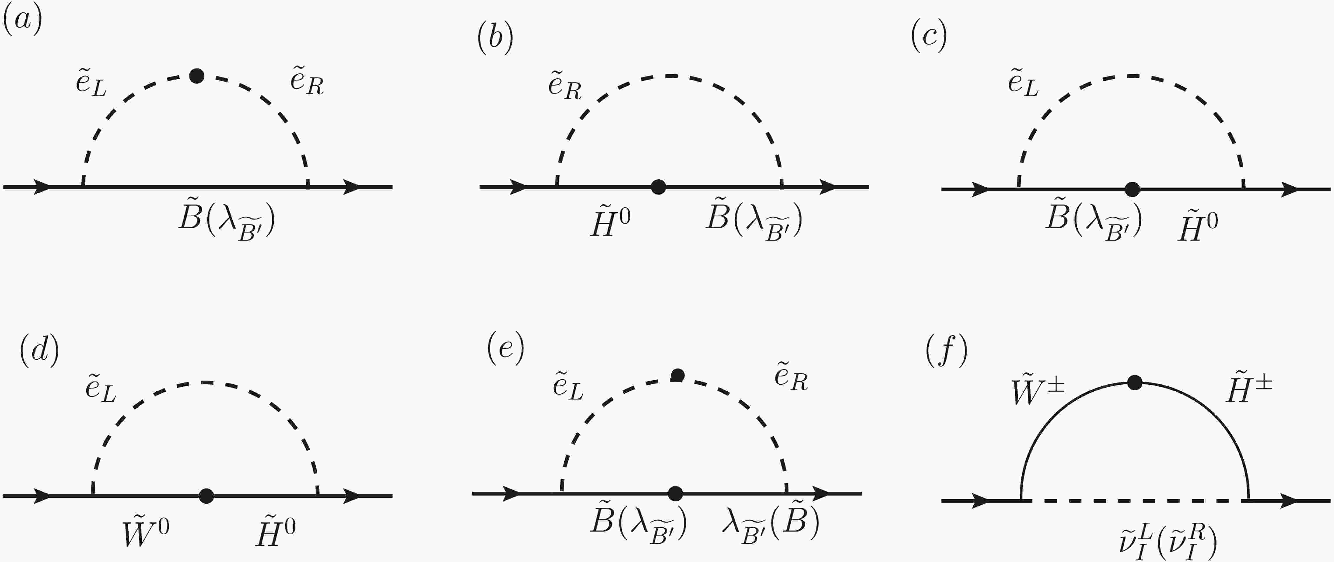
In the N-B-LSSM, the one-loop corrections to the lepton electric dipole moment primarily arise from loop diagrams involving sleptons and gauginos, such as the neutralino $ \chi^0 $ and chargino $ \chi^\pm $, together with new-physics parameters. Moreover, the introduction of right-handed neutrino superfields makes the sneutrino mass spectrum and mixing structure more complicated and may provide additional sources of CP violation. The EDM contributions are generally not proportional to a single mass ratio; instead, they are constrained by mixing matrix elements. Their magnitudes are highly sensitive to new CP-violating phases and to model parameters such as $ \tan\beta $. To clarify this parameter dependence, it is particularly convenient to employ the MIA [34], which expresses the EDM contributions analytically as functions of the model parameters and thereby highlights the origin of CP violation. Fig. 1 shows the Feynman diagrams for the lepton EDM obtained using the MIA.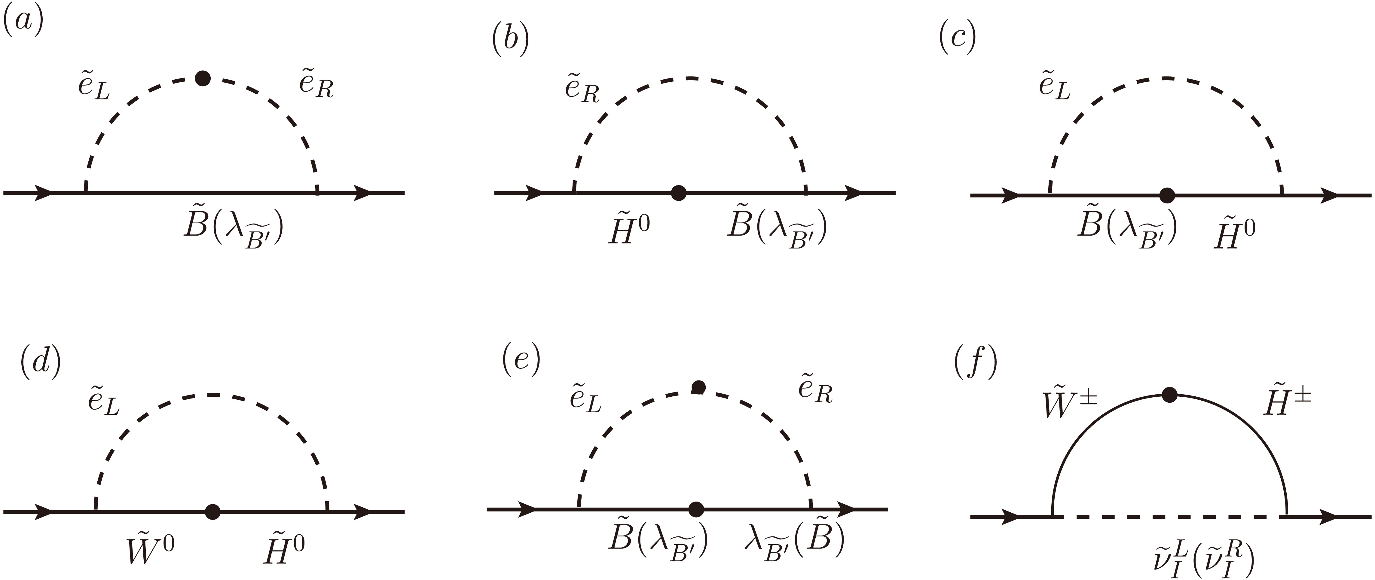

Figure 1.  Feynman diagrams for generating the lepton EDM within the MIA. The external photons are attached to the charged internal lines in all possible ways.

The MIA provides a powerful framework for analyzing supersymmetric CP-violating observables. The EDM contributions from neutralino-slepton, chargino-sneutrino, and gluino–squark loop diagrams have been extensively studied within the MSSM framework [35–37]. Compared with the MSSM, the N-B-LSSM contains additional CP-violating sources, including the additional $ U(1)_{B-L} $ gaugino mass ($ M_{BL} $), the mass mixing term ($ M_{BB'} $) between the $ U(1)_{Y} $ gaugino and the $ U(1)_{B-L} $ gaugino, and the mass and mixing terms of the superpartners of the Higgs singlets $ \chi_1 $, $ \chi_2 $, and S. Furthermore, the new gauge coupling parameters $ g_B $ and $ g_{YB} $ can significantly affect the EDM corrections. Below, within the N-B-LSSM and using the MIA, we present the explicit analytical forms of the one-loop contributions to the lepton EDM.

a. One-loop contributions from $ \widetilde{B} $-$ \tilde{e}_L $-$ \tilde{e}_R $ and $ \lambda_{\tilde{B'}} $-$ \tilde{e}_L $-$ \tilde{e}_R $.

Here, $ x_i=\dfrac{|m_i|^2}{M^2_{SUSY}} $, where $ M_{SUSY} $ denotes the supersymmetric mass scale.

The function $ I_1(x,y,z) $ is defined as

b. One-loop contributions involving $ \widetilde{B} $-$ \widetilde{H}^0 $-$ \tilde{e}_R $ and $ \lambda_{\tilde{B'}} $-$ \widetilde{H}^0 $-$ \tilde{e}_R $.

c. One-loop contributions from $ \widetilde{B} $-$ \widetilde{H}^0 $-$ \tilde{e}_L $ and $ \lambda_{\tilde{B'}} $-$ \widetilde{H}^0 $-$ \tilde{e}_L $.

d. One-loop contributions from $ \widetilde{W}^0 $-$ \widetilde{H}^0 $-$ \tilde{e}_L $.

The function $ I_2(x,y,z) $ is defined as

e. The one-loop contributions from the $ \lambda_{\tilde{B'}} $-$ \widetilde{B} $-$ \tilde{e}_L $-$ \tilde{e}_R $ and $ \widetilde{B} $-$ \lambda_{\tilde{B'}} $-$ \tilde{e}_L $-$ \tilde{e}_R $ diagrams.

The functions $ f(x,y,z,t) $ and $ g(x,y,z,t) $ are defined as follows:

f. One-loop contributions arising from $ \widetilde{W}^\pm $-$ \widetilde{H}^\pm $-$ \widetilde{\nu}_L^I $ and $ \widetilde{W}^\pm $-$ \widetilde{H}^\pm $-$ \widetilde{\nu}_L^R $.

The function $ I_3(x,y,z) $ is defined as

The one-loop contributions to the lepton EDM can be expressed as

The neutron EDM can also be obtained from the effective Lagrangian in Eq. (12). The neutron is a composite particle consisting of quarks and gluons. Its EDM arises not only from the quark EDM but also from important contributions from the quark CEDM. This contribution is described by the operator $ \bar{q} T^a \sigma_{\mu\nu} \gamma_5 q G_a^{\mu\nu} $, where $ G_a^{\mu\nu} $ is the gluon field-strength tensor.

The one-loop diagrams that generate the neutron EDM and CEDM based on the MIA are shown in Fig. 2. Fig. 1(e) and Fig. 2(d), (e) differ from the other one-loop diagrams because they involve two distinct neutral gauginos connected through the soft-mixing mass parameter $ M_{BB'} $. In the N-B-LSSM, $ M_{BB'} $ is a distinctive parameter and represents an important feature of the N-B-LSSM compared with the MSSM. The presence of $ M_{BB'} $ gives rise to additional contributions associated with the extended neutralino sector. Accordingly, when the relevant couplings and mass parameters carry complex phases, this class of diagrams induces additional CP-violating contributions associated with the extended gauge sector, which are absent in the MSSM. Therefore, these diagrams constitute an important component of the complete EDM calculation in the N-B-LSSM.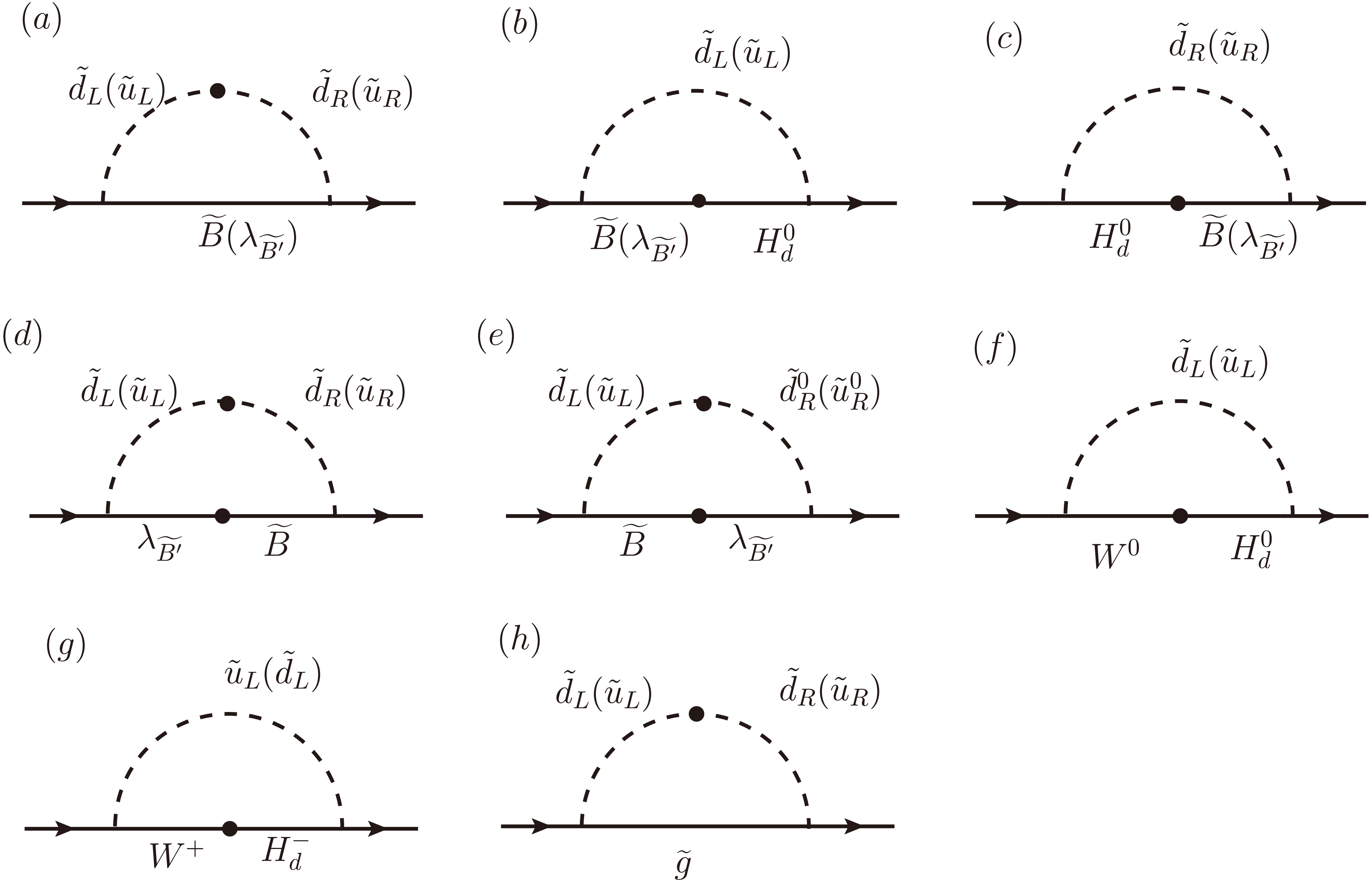

Figure 2.  Quark Feynman diagrams contributing to the generation of neutron EDMs and CEDMs under the MIA. External photons are attached to charged internal lines in all allowed insertion configurations, whereas external gluons couple to the colored internal lines in the loop diagrams.

a. The one-loop EDM contributions to the up and down quarks induced by the $ \widetilde{B} $-$ \tilde{q}_L $-$ \tilde{q}_R $ and $ \lambda_{\widetilde{B'}} $-$ \tilde{q}_L $-$ \tilde{q}_R $ loop diagrams are given by

with $ q=u,\; d $, $ A_d=\tan\beta $, $ A_u=4 $, $ B_d=(-2g_{YB}+g_B)\tan\beta $, and $ B_u=-2(4g_{YB}+g_B) $.

The one-loop CEDM contributions for the up and down quarks induced by the $ \widetilde{B} $-$ \tilde{q}_L $-$ \tilde{q}_R $ and $ \lambda_{\widetilde{B'}} $-$ \tilde{q}_L $-$ \tilde{q}_R $ loop diagrams are given by

b. The one-loop EDM contributions to quarks (the u and d quarks) induced by the $ \widetilde{B} $-$ \widetilde{H}^0 $-$ \tilde{q}_L $ and $ \lambda_{\widetilde{B'}} $-$ \widetilde{H}^0 $-$ \tilde{q}_L $ loop diagrams are given by

with $ C_d=\tan\beta,\; C_u=-2 $, $ D_d=g_{YB}\tan\beta $, and $ D_u=-2g_{1} $.

The one-loop CEDM contributions to the up and down quarks induced by the $ \widetilde{B} $-$ \widetilde{H}^0 $-$ \tilde{q}_L $ and $ \lambda_{\widetilde{B'}} $-$ \widetilde{H}^0 $-$ \tilde{q}_L $ loop diagrams are given by

c. The one-loop EDM contributions to quarks (the u and d quarks) induced by the $ \widetilde{B} $-$ \widetilde{H}^0 $-$ \tilde{q}_R $ and $ \lambda_{\widetilde{B'}} $-$ \widetilde{H}^0 $-$ \tilde{q}_R $ loop diagrams are given by

where $ E_d=\tan\beta,\; E_u=-4 $, $ F_d=g_{YB}(-2g_{YB}+g_B)\tan\beta $, and $ F_u=-2g_1(4g_{YB}+g_B) $.

The one-loop CEDM contributions to the up and down quarks induced by the $ \widetilde{B} $-$ \widetilde{H}^0 $-$ \tilde{d}_R $, $ \widetilde{B} $-$ \widetilde{H}^0 $-$ \tilde{q}_R $, and $ \lambda_{\widetilde{B'}} $-$ \widetilde{H}^0 $-$ \tilde{q}_R $ loop diagrams are given by

d. The one-loop EDM and CEDM contributions to the quarks (the u and d quarks), induced by the $ \lambda_{\widetilde{B'}} $-$ \widetilde{B} $-$ \tilde{q}_L $-$ \tilde{q}_R $ loop diagrams, are given by

The one-loop EDM and CEDM contributions to the u and d quarks induced by the $ \widetilde{B} $-$ \lambda_{\widetilde{B'}} $-$ \tilde{q}_L $-$ \tilde{q}_R $ loop diagrams are given by

with $ G_d=(-2g_{YB}+g_B)\tan\beta $ and $ G_u=-8(4g_{YB}+g_B) $.

f. The one-loop EDM and CEDM contributions to the quarks (the u and d quarks) induced by the $ \widetilde{W}^0 $-$ \widetilde{H}^0 $-$ \widetilde{q}_L $ loop diagrams are given by

with $ H_d=\tan\beta $ and $ H_u=2 $.

The one-loop EDM and CEDM contributions to the u and d quarks induced by the $ \widetilde{W}^\pm $-$ \widetilde{H}^\pm $-$ \widetilde{q}_L $ loop diagrams are given by

where $ I_d=\tan\beta $ and $ I_u=\dfrac{1}{2} $. The functions $ I_4(x,y,z) $ and $ I_5(x,y,z) $ are defined as follows:

The one-loop contributions to the EDMs and CEDMs of quarks (the u and d quarks) induced by the $ \lambda_{\widetilde{g}} $-$ \widetilde{q}_L $-$ \widetilde{q}_R $ loop diagrams are given by

The function $ I_6(x,y,z) $ is defined as

We define the parameters that may have CP-violating phases as follows:

$ \theta_1 $, $ \theta_2 $, $ \theta_{\mu_H} $, $ \theta_{1'} $, and $ \theta_{BB'} $ are the CP-violating phases.

Both the quark EDM and CEDM contribute to the neutron EDM. We use the following expression [38]

Using lattice QCD [39] at a renormalization scale of 2 GeV, the tensor charges have been obtained as $ g^u_T= -0.233(28),\; g^d_T=0.774(66) $, and $ g^s_T=0.009(8) $. To improve the reliability of the results, the authors also calculated these quantities at a renormalization scale of 2 GeV using QCD sum rules [40]. The results obtained from the two approaches (lattice QCD and QCD sum rules) differ [41], which may slightly affect the coefficients in Eq.(58). Nevertheless, this does not qualitatively influence the results. For the neutron EDM, we can safely neglect the corrections from the CEDMs of heavy quarks. Even the contribution from the strange quark can be safely neglected because $ g_T^s\ll g_T^d $.

In our previous work [42], we numerically compared the MIA and mass-eigenstate results in detail for the muon anomalous magnetic moment within the framework of the BLMSSM. For different parameters varied over wide ranges, the relative error $ \left|\dfrac{a_\mu^{MIA}-a_\mu^{ME}}{a_\mu^{MIA}}\right| $≤10%. Within the common range of values, the relative error is not larger than 5%. In this work, the relative error between the MIA results and the mass-eigenstate results lies in the range 2.5% ~ 5.0%. Overall, the MIA is reliable.

When performing the calculations, the following experimental constraints are taken into account.

1. The experimental constraint on the lightest CP-even Higgs mass, $ 125.20\pm0.11 $ $ {\rm{GeV}} $, is considered [11, 43, 44].

2. The $ Z^\prime $ boson mass should be larger than 5.1 TeV. The ratio between $ M_{Z^\prime} $ and its gauge coupling, $ M_{Z^\prime}/g_B $, should be not smaller than $ 6 \; {{\rm{TeV}}} $ [45].

3. The new angle $ \beta_\eta $ is constrained by the LHC as $ \tan\beta_\eta<1.5 $ [46].

4. The constraints on the particle masses are as follows [47–52]. The neutralino mass is constrained to be greater than 116 GeV, the chargino mass is constrained to be greater than 900 GeV, and the slepton masses are of order TeV. The squark mass should not be smaller than 1500 GeV. The gluino mass should be larger than 2000 GeV.

5. The experimental results for $ \bar{B}\to X_s\gamma $ impose stringent constraints on the value of $ \tan\beta $. The Yukawa coupling of the bottom quark reads $ Y_b=\sqrt{2(1+\tan^2\beta)}\,\dfrac{m_b}{v}. $ With the parameter values $ m_b\simeq 4.18\ {\rm{GeV}} $ and $ v\simeq 246\ {\rm{GeV}} $, we require $ \tan\beta \lesssim 40 $ to satisfy the condition $ Y_b<1 $.

To obtain the numerical results in this work, the relevant parameters are set as follows. $ v_{S}=2\; {{\rm{TeV}}} $, $ \lambda=0.25 $, $ M_{SUSY}=1500\; {{\rm{GeV}}} $, $ m_{\tilde{W}^0}=900\; {{\rm{GeV}}} $, $ m_{\tilde{u}_L}=1800\; {{\rm{GeV}}} $, $ m_{\tilde{u}_R}=2000\; {{\rm{GeV}}} $.

Leptons are elementary particles. Their EDMs directly characterize CP-violation effects in fundamental interactions and depend strongly on the lepton masses. The τ-lepton, the heaviest lepton, is the most sensitive to CP violation. The electron, the lightest lepton, has an extremely weak EDM signal that requires sophisticated detection techniques. The μ-lepton lies in the intermediate response range. Within the MIA, the EDM can be expressed as an analytic combination of various mass insertion parameters and the imaginary parts of CP-violating phases. Thus, it exhibits clear parametric responses to the gauge coupling constants $ g_{\text{YB}} $ and $ g_{\text{B}} $, the Higgs vacuum structure $ \tan\beta $, and the independent CP phases $ \theta_{\mu_H} $ and $ \theta_{1} $.

Fig. 3(a) shows the variation of $ |d_\tau| $ with $ g_{YB} $ for different values of $ \tan\beta $. The phase is set to $ \theta_{\mu_H}=\dfrac{\pi}{3} $, and the other phases are set to $ \theta_{1}=\theta_{2}=\theta_{1'}=\theta_{BB'}=0 $. In the range $ 0 \le g_{YB} \le 0.60 $, $ |d_\tau| $ exhibits an approximately linear increase with $ g_{YB} $, indicating that this gauge interaction enhances the EDM of the τ lepton. For the same value of $ g_{YB} $, increasing $ \tan\beta $ leads to an overall increase in $ |d_\tau| $. Fig. 3(b) presents the variation of $ d_\tau $ with $ \theta_{\mu_H} $ for different values of $ \tan\beta $. The other phases are set to $ \theta_{1}=\theta_{2}= \theta_{1'}=\theta_{BB'}=0 $. $ d_\tau $ exhibits a sinusoidal dependence on $ \theta_{\mu_H} $ with a period of $ 2\pi $, with zeros located at $ \theta_{\mu_H}=0, \pi, 2\pi $. As $ \tan\beta $ increases, the oscillation amplitude increases significantly, whereas the zero-crossing positions remain unchanged. This indicates that $ \tan\beta $ does not change the phase structure but affects only the contribution of the phase-dependent term to the total amplitude. $ \theta_{\mu_H} $ provides a new CP-violating source independent of the CKM phase in the SM. The obtained values of $ d_\tau $ are consistent with current experimental constraints, being approximately three orders of magnitude below the experimental upper limit.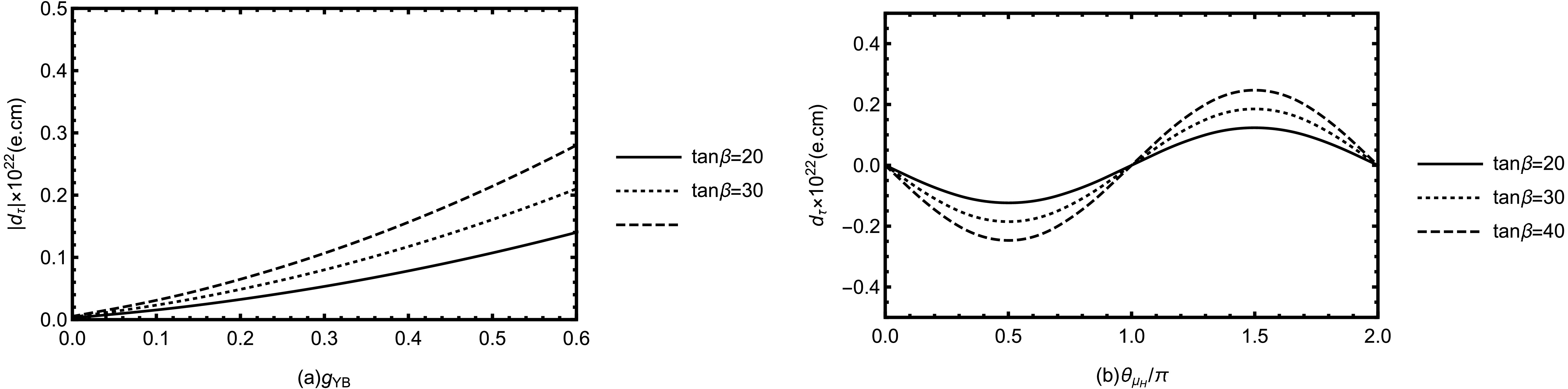

Figure 3.  Effects of $ g_{YB} $, $ \theta_{\mu_H} $, and $ \tan\beta $ on $ d_{\tau} $

Figure 4(a) illustrates the variation of $ |d_\mu| $ with $ |g_{YB}| $ for different values of $ \tan\beta $. The phase $ \theta_{\mu_H} $ is set to $ \frac{\pi}{3} $, and the other phases are set to $ \theta_{1}=\theta_{2}=\theta_{\mu_H}=\theta_{1'}=\theta_{BB'}=0 $. In the range $ 0 \leq |g_{YB}| \leq 1.0 $, $ |d_\mu| $ first increases slightly and then decreases to zero as $ |g_{YB}| $ increases. This behavior indicates a mutual cancellation effect between the contributions of different loop diagrams within this parameter range. For $ |g_{YB}| \in [0.4, 1.0] $, $ |d_\mu| $ resumes a monotonically increasing trend, and the growth rate accelerates with increasing $ \tan\beta $. Figure 4(b) depicts the dependence of $ d_\mu $ on the phase $ \theta_1 $ for $ \tan\beta = 20, 30, 40 $. The other phases are set to $ \theta_{2}=\theta_{\mu_H}=\theta_{1'}=\theta_{BB'}=0 $. Similar to the case of the τ lepton, $ d_\mu $ exhibits a typical sinusoidal oscillation with a period of $ 2\pi $ as $ \theta_1 $ varies, with zeros at $ \theta_1 = 0, \pi, 2\pi $. This behavior reflects the periodic dependence of amplitude interference on this CP-violating phase. Increasing $ \tan\beta $ significantly enhances the oscillation amplitude. This demonstrates that $ \tan\beta $ does not alter the phase structure itself but enhances the observable strength of the CP-violating effect by increasing the relevant Yukawa couplings. As a CP-violating source independent of the CKM phase in the SM, the sizable signal induced by $ \theta_1 $ in the lepton EDM provides a promising avenue for probing new physics CP phases in higher-precision experiments.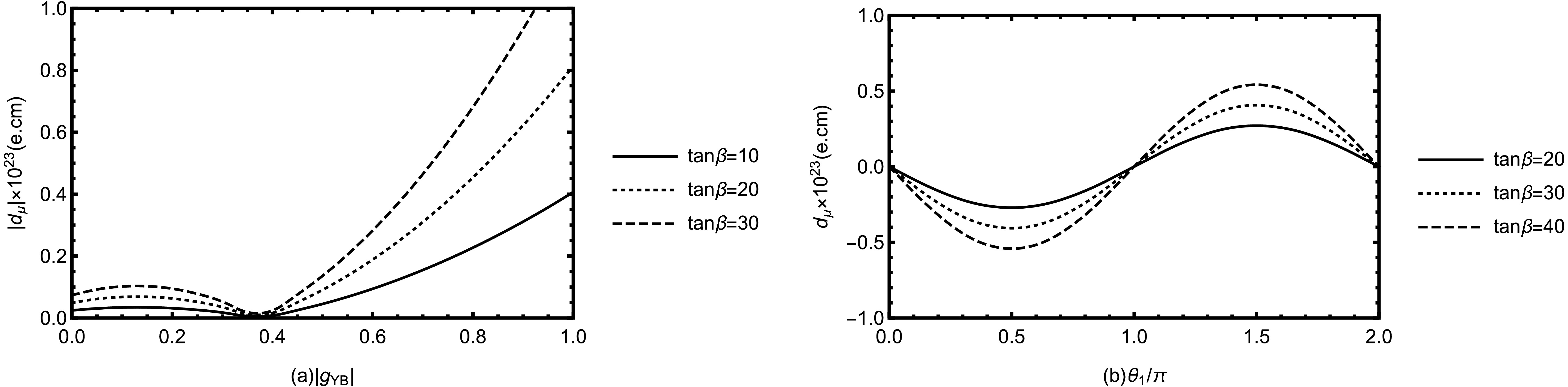

Figure 4.  Effects of $ g_{YB} $, $ \theta_{1} $, and $ \tan\beta $ on $ d_{\mu} $.

The experimental upper limit on the electron EDM ($ d_e $) is highly stringent. To ensure that the $ d_e $ values predicted by the N-B-LSSM within the framework of the MIA satisfy this constraint, three commonly used suppression mechanisms are adopted: (1) choosing small CP-violating phases; (2) increasing the masses of the relevant new particles to suppress loop amplitudes; and (3) exploiting internal cancellations among contributions from distinct phases, thereby reducing the imaginary-part contributions without violating the phase structure.

a. Small CP-violating phases Fig. 5 depicts the behavior of the electron EDM $ |d_e| $ for a small CP-violating phase. In this case, $ \theta_{1'}= \dfrac{\pi}{1000} $, and the other phases are set to $ \theta_{1}=\theta_{2}=\theta_{\mu_H}=\theta_{BB'}=0 $. As shown in the figure, as $ g_B $ increases from 0 to approximately 0.6, $ |d_e| $ decreases monotonically and reaches a minimum at $ g_B \approx 0.6 $. This indicates that increasing $ g_B $ changes the relative weights of the various loop contributions, thereby suppressing $ |d_e| $ within this region. Beyond $ g_B \approx 0.6 $, $ |d_e| $ increases significantly, demonstrating that $ g_B $ has a crucial influence on $ |d_e| $ in the small-phase-angle limit. Different values of $ \tan\beta $ (8, 10, 12) affect only the overall magnitude of $ |d_e| $ at each $ g_B $, without changing the overall trend.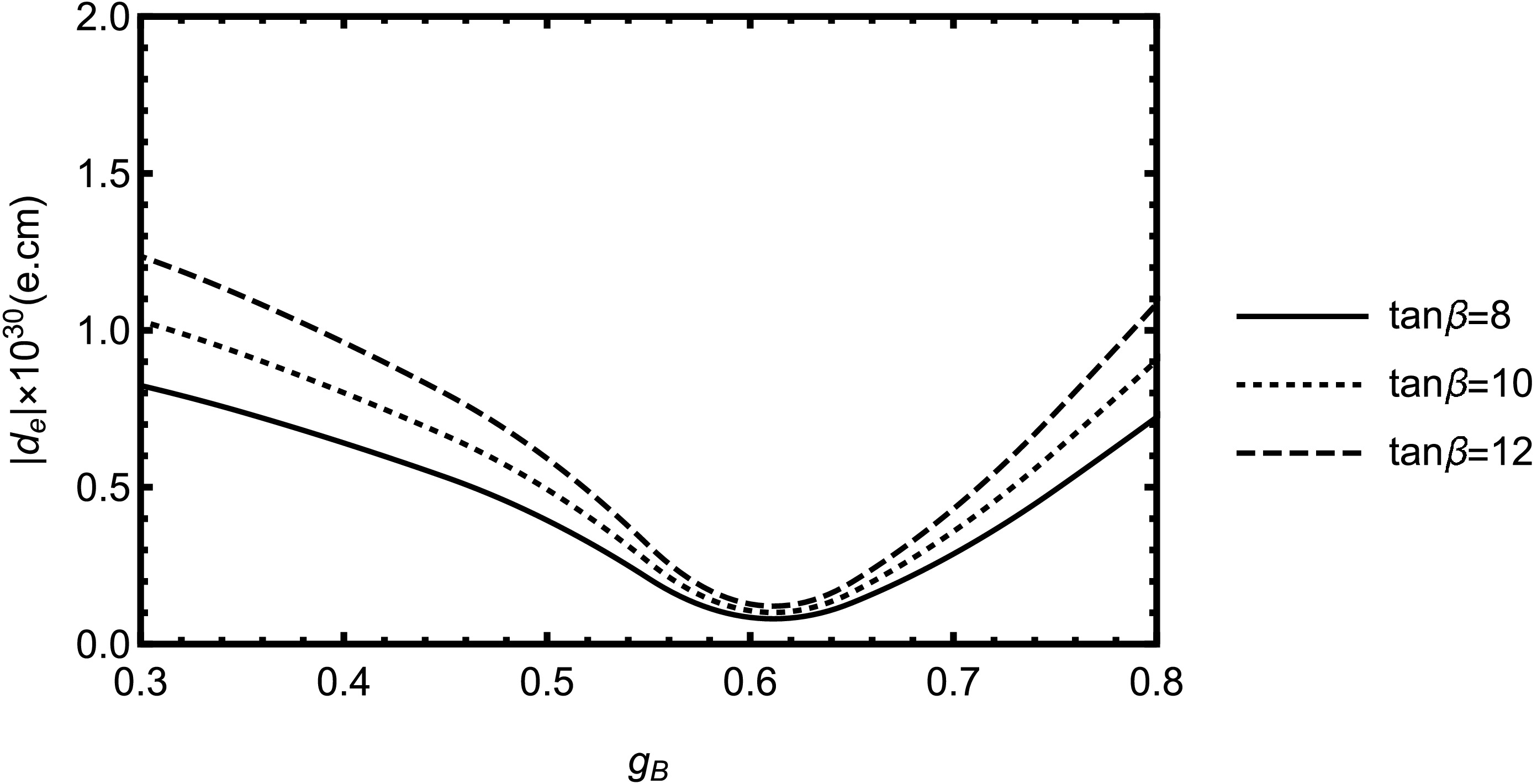

Figure 5.  Effects of $ g_{B} $ and $ \tan\beta $ on $ d_{e} $.

b. large-mass approach In Fig. 6, we perform calculations using the large-mass approach ($ m_{\widetilde{e_L}}=13000\ \text{GeV} $, $ m_{\widetilde{e_R}}=14000\ \text{GeV} $) for $ \tan\beta=5 $, 10, and 15. The phases are set to $ \theta_{2}=\theta_{\mu_H}=\theta_{1'}=\theta_{BB'}=0 $. The electron EDM $ d_e $ still exhibits sinusoidal oscillations with a $ 2\pi $ period as a function of $ \theta_1 $, consistent with the patterns observed for the τ and μ leptons. However, the oscillation amplitude is extremely small. Heavy sleptons reduce only the magnitude of $ d_e $ without eliminating the phase effect. Slepton masses of order 10 TeV, combined with a normal phase, can satisfy the experimental constraints on $ d_e $. Nevertheless, this conflicts with the principle of naturalness.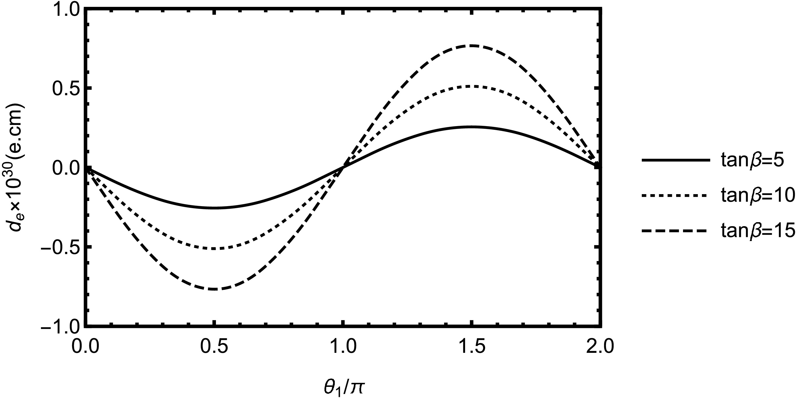

Figure 6.  Effects of $ \theta_1 $ and $ \tan\beta $ on $ d_{e} $.

c. The phase cancellation mechanism In Fig. 7, we illustrate the phase cancellation mechanism by scanning the mass parameter $ m_{\tilde{B}} $. In this case, the phases are set to $ \theta_1=\dfrac{\pi}{20} $, $ \theta_{1'}=\dfrac{\pi}{20} $, and $ \theta_{2}=\theta_{\mu_H}=\theta_{BB'}=0 $. The electron EDM $ d_e $ exhibits a clear V-shaped distribution, with a near-zero optimal cancellation point around $ m_{\tilde{B}}\simeq 1100\ \text{GeV} $. As $ \tan\beta $ decreases, the V-shaped structure generally becomes deeper and wider. This indicates that smaller values of $ \tan\beta $ increase the relative weight of phase-related terms in the total amplitude. Thus, this cancellation mechanism can accommodate CP-violating phases of typical size while keeping the particle masses in the TeV range. The resulting predictions are also more likely to satisfy the experimental limits.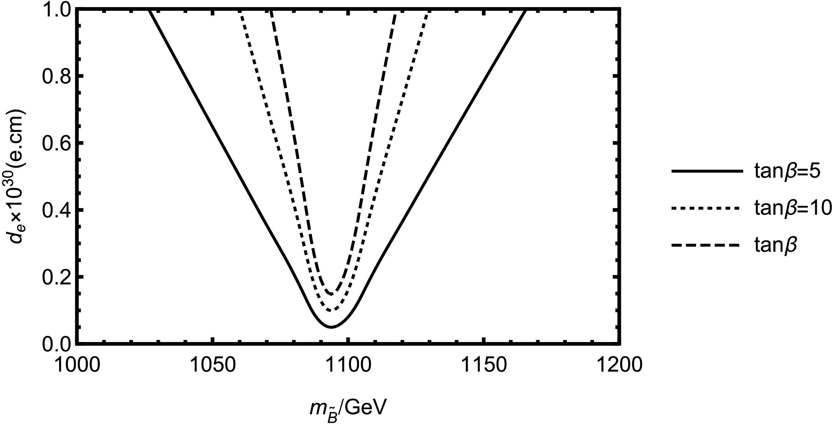

Figure 7.  Effects of $ m_{\tilde{B}} $ and $ \tan\beta $ on $ d_{e} $.

Leptons are fundamental particles, whereas neutrons are composite particles. In contrast to lepton EDMs, the neutron EDM arises from CP-violating interactions at the quark and gluon levels and receives contributions from quark EDMs and CEDMs. Consequently, it has more intricate dependencies on the model parameters.

In Fig. 8(a), we study the dependence of the neutron EDM $ |d_n| $ on $ m_{\tilde{B}} $. The CP phases are fixed as $ \theta_{2}=\theta_{3}= \theta_{\mu_H}=\theta_{1'}=\theta_{BB'}=0 $, with only the CP-violating phase $ \theta_1 $ retained. We find that $ |d_n| $ decreases monotonically with increasing $ m_{\tilde{B}} $ for different values of $ \theta_1 $. The phase $ \theta_1 $ mainly affects the overall magnitude of the EDM, whereas the dependence on $ m_{\tilde{B}} $ remains unchanged. The decrease in $ |d_n| $ with increasing $ m_{\tilde{B}} $ can be attributed to the mass suppression of the loop contributions, indicating decoupling behavior. Fig. 8(b) shows the dependence of $ |d_n| $ on the gluino mass $ m_g $ for $ \theta_3=\dfrac{\pi}{10},\dfrac{\pi}{15},\dfrac{\pi}{20} $, where the other CP phases are set to $ \theta_{1}=\theta_{2}=\theta_{\mu_H}=\theta_{1'}=\theta_{BB'}=0 $. The neutron EDM increases with $ m_g $, and a larger $ \theta_3 $ leads to a larger value of $ |d_n| $. The rate of increase gradually decreases. This indicates that the gluino-related contribution is sensitive to the CP-violating phase $ \theta_3 $. The shaded region denotes the experimentally allowed range of the neutron EDM, which constrains the relevant parameter space of the N-B-LSSM.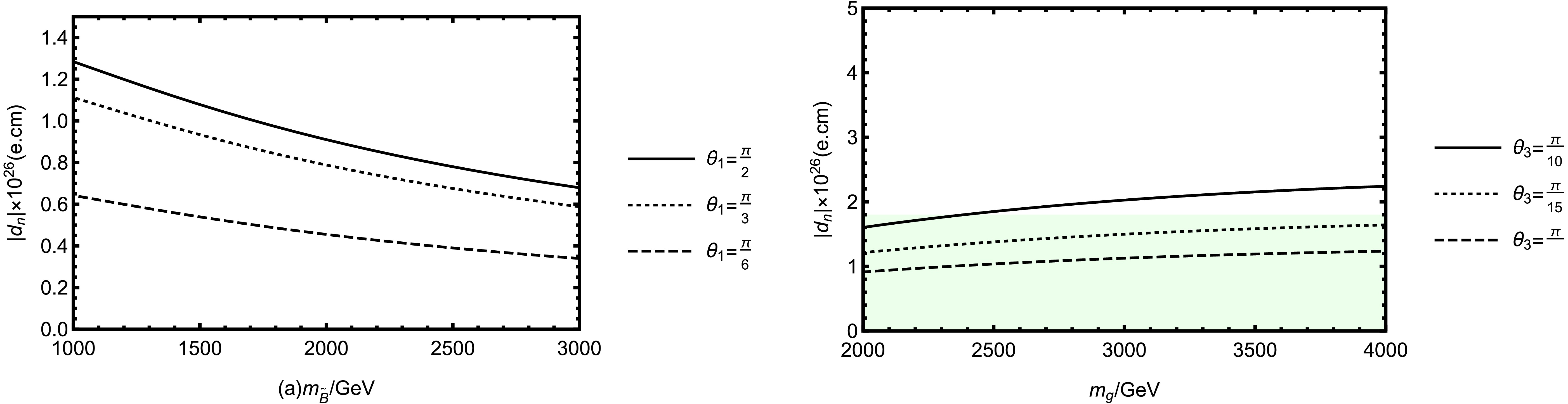

Figure 8.  The effects of $ m_{B} $ and $ \theta_{1} $, as well as $ m_{g} $ and $ \theta_{3} $, on $ d_{n} $.

Fig. 9(a) shows the dependence of the scaled neutron EDM, $ d_n\times10^{26} $, on the CP-violating phase $ \theta_3 $ for different values of $ \tan\beta $, with $ \theta_{1}=\theta_{2}=\theta_{\mu_H}=\theta_{1'}=\theta_{BB'}=0 $. The neutron EDM exhibits periodic oscillatory behavior as $ \theta_3 $ varies from 0 to $ 2\pi $. The EDM vanishes at $ \theta_3=0,\pi,2\pi $, corresponding to the CP-conserving points. Furthermore, the oscillation amplitude increases with $ \tan\beta $, indicating an enhancement of the CP-violating contribution to the neutron EDM. The shaded region denotes the experimentally allowed range. Fig. 9(b) presents the dependence of the neutron EDM on the CP-violating phase $ \theta_{1'} $, with $ \theta_{1}=\theta_{2}=\theta_{\mu_H}=\theta_{3}=\theta_{BB'}=0 $. The EDM shows similar periodic behavior with respect to $ \theta_{1'} $. However, the oscillation amplitude is much smaller than that induced by $ \theta_3 $, indicating that the contribution associated with $ \theta_{1'} $ is relatively suppressed in the neutron EDM calculation.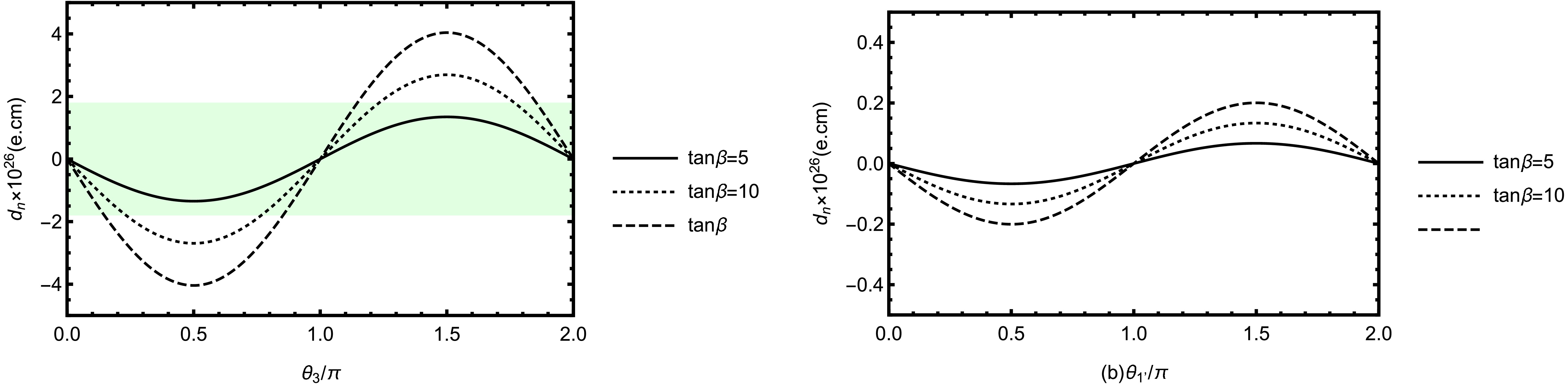

Figure 9.  The effects of $ \theta_3 $ and $ \tan\beta $, and of $ \theta_{1'} $ and $ \tan\beta $, on $ d_{n} $.

Fig. 10 presents the allowed parameter regions in the $ m_{\lambda_{B'}}-\theta_{1'} $ plane for different ranges of the neutron EDM $ d_n $. The different colors correspond to different intervals of the predicted EDM values. The neutron EDM is sensitive to the CP-violating phase $ \theta_{1'} $. Relatively large values of $ d_n $ are mainly located in the region $ \theta_{1'}\sim(0.3\pi-0.7\pi) $, where the CP-violating contribution is enhanced. When $ \theta_{1'} $ approaches the CP-conserving regions, the predicted EDM values are suppressed. In addition, the region with larger EDM values becomes narrower as $ m_{\lambda_{\widetilde{B}'}} $ increases, indicating suppression due to the heavy mass.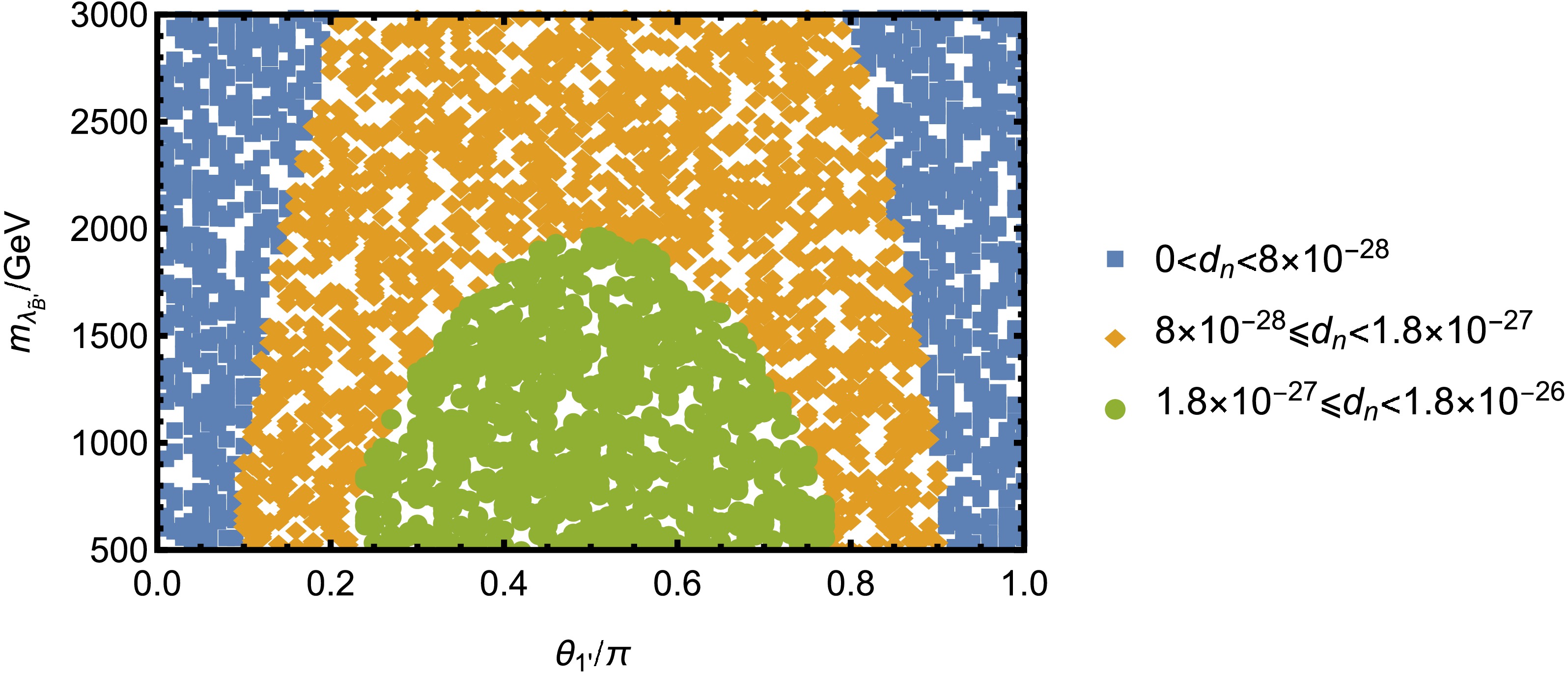

Figure 10.  Effects of $ m_{\lambda_{\widetilde{B}'}} $ and $ \theta_{1'} $ on $ d_{n} $ (in units of e.cm) for $ m_{\widetilde{d}_L}=2100\; \text{GeV} $, $ m_{\widetilde{d}_R}=1900\; \text{GeV} $, and $ m_g=2500\; \text{GeV} $.

As shown in Fig. 11, for the CP-violating phase $ \theta_1=\frac{\pi}{6} $ and the other phases $ \theta_{2}=\theta_{3}=\theta_{\mu_H}=\theta_{1'}=\theta_{BB'}=0 $, the larger EDM values (green region) are mainly distributed in the parameter region with relatively small $ m_{\widetilde{d}_L} $ and $ m_{\widetilde{d}_R} $. When both mass parameters are small, the corresponding supersymmetric loop contributions are less suppressed, resulting in larger neutron EDM values. As $ m_{\widetilde{d}_L} $ or $ m_{\widetilde{d}_R} $ increases, the predicted $ d_n $ gradually decreases, indicating that larger masses suppress the relevant loop corrections. The different colored regions in Fig. 11 represent the predicted neutron EDM values for different combinations of $ m_{\widetilde{d}_L} $ and $ m_{\widetilde{d}_R} $. By imposing the current experimental upper bound on the neutron EDM, the parameter regions predicting relatively large EDM values (green region) can be excluded, leading to further constraints on the allowed ranges of $ m_{\widetilde{d}_L} $ and $ m_{\widetilde{d}_R} $.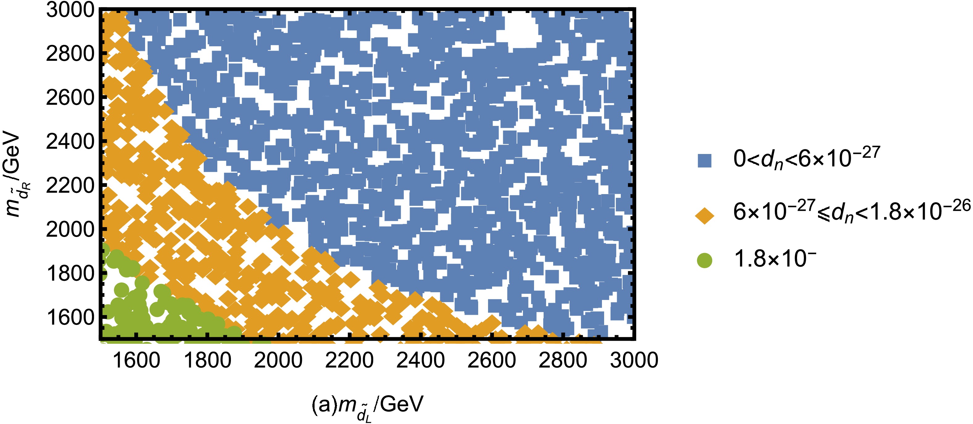

Figure 11.  Dependence of $ d_{n} $ (in units of $ e\cdot{\rm{cm}} $) on $ m_{\widetilde{d}_L} $ and $ m_{\widetilde{d}_R} $, with $ m_g= 2500\; \text{GeV} $ and $ m_{\lambda_{\widetilde{B}'}}= 3000\; \text{GeV} $.

Within the framework of the N-B-LSSM, we systematically calculate the one-loop contributions to the lepton and quark EDMs via the MIA and perform a comprehensive numerical analysis. This study reveals the modulatory effects of kinetic mixing parameters and new CP-violating phases on EDMs.

In the lepton sector, the coupling parameter $g_{YB}$ can modify the relative weights of different one-loop contributions and induce regions of destructive interference. Phase parameters of the $\theta$-type exhibit typical periodic oscillations of EDMs with a $ 2\pi $ cycle. In contrast, $ \tan\beta $ increases the overall magnitude of EDMs primarily by enhancing the weights of chiral mixing, without changing the distribution of EDM zero points. Under stringent experimental constraints, the electron EDM can be effectively suppressed by small phase values, high mass scales, or phase cancellation mechanisms. Notably, the phase cancellation mechanism allows large CP-violating phases to exist even when the particle mass is at the TeV scale, thereby improving the viability of the model.

The neutron EDM receives contributions from quark EDMs and quark CEDMs, leading to richer parameter-dependent features. $ \tan\beta $ has a stable enhancement effect on the neutron EDM, whereas the newly introduced mass scale shows a suppressive trend. The strong phase $ \theta_3 $ usually dominates the structure of CP interference, while other phases, such as $ \theta_{1'} $, constitute secondary but independent sources of CP violation.

EDM experiments impose stringent joint constraints on the kinetic mixing coupling parameters and new CP-violating phases in the N-B-LSSM. In particular, high-precision measurements of the electron and neutron EDMs provide a clear observational window for testing this class of $ U(1)_{B-L} $ extended supersymmetric models.

With a reasonable selection of parameters, the N-B-LSSM can simultaneously satisfy the current experimental upper limits on lepton and neutron EDMs, and certain parameter spaces can even approach the detection sensitivity of future experiments. The MIA is well suited to this model and enables a clear elucidation of the roles of CP-violating phases and various coupling parameters in EDMs. This work establishes a complete analytical framework and numerical benchmark for the systematic study of EDMs in B-L extended supersymmetric models and provides solid theoretical support for probing CP-violating phases in new physics through future high-precision EDM experiments.