Hawking radiation from non-minimal Einstein–Yang–Mills black holes

Hawking radiation is shaped by two distinct aspects of the black-hole problem. The first is local thermodynamics: the surface gravity determines the temperature of the near-horizon state. The second is scattering: outgoing modes must cross a curvature-induced potential barrier before reaching infinity. The corresponding transmission probabilities, or greybody factors, determine the observable spectrum and the integrated luminosity [1−4]. For black holes whose geometry differs from Schwarzschild only near the horizon or in the deep interior, these two effects need not vary in the same direction. A barrier may become slightly more transparent while the temperature decreases, or vice versa.

This competition is especially important for regular black holes and for black holes in effective theories with non-minimal matter-curvature couplings. In such geometries, the central singularity can be replaced by a finite core, and the black-hole branch often terminates at a zero-temperature extremal state. Greybody factors then address a concrete question: does the modified exterior geometry enhance the outgoing flux, or is evaporation mainly quenched by the cooling of the horizon? Greybody factors of black holes have therefore been examined recently in numerous studies [5−26].

Here we address this question for the non-minimal Einstein–Yang–Mills black hole derived by Balakin and Zayats and later embedded in a cosmological-constant family by Balakin, Lemos and Zayats [27, 28]. The same spacetime was recently studied in terms of scalar quasinormal modes and scalar greybody factors; the fundamental mode was found to be comparatively stable, whereas the overtones are much more sensitive to the non-minimal coupling [29]. We use that work as the starting point but shift the focus from ringing to Hawking emission. Although lower bounds on the greybody factors for this case were estimated in [30], the greybody factors themselves have not been calculated to date.

Our aim is to follow a Page-type program for the non-minimal Yang–Mills background. We determine the horizon and temperature, compute direct-integration greybody factors for scalar, electromagnetic, and massless Dirac test channels, compare the dominant thresholds with a barrier-top WKB estimate, and integrate the Hawking spectra. The scalar channel is included because the recent quasinormal-mode analysis used scalar perturbations. The electromagnetic field and three copies of the neutral massless Dirac result define a restricted photon-plus-light-fermion proxy; they do not represent the complete Standard Model particle content.

Throughout the paper we use natural units $ G= c=\hbar=k_B=1 $. This convention fixes the conversion between length, time, mass and temperature. The black-hole family is characterized by the ADM mass M, the magnetic Yang–Mills charge Q, and the non-minimal curvature-coupling scale ξ, while ω denotes the real scattering frequency, $ T_H $ the Hawking temperature, and P an integrated luminosity. When numerical values are quoted, all dimensionful quantities are expressed in units of the black-hole mass; for example, radii, charges, frequencies, temperatures and powers are reported through the corresponding dimensionless combinations. The detailed benchmark branches are specified below. The main result is that the non-minimal coupling raises the dominant greybody thresholds only mildly, but it drives the temperature and luminosity sharply downward near the cold endpoint. Below we test the respective roles of cooling and transmission directly. Cooling supplies the largest part of the many-orders-of-magnitude suppression, although the altered low-frequency greybody factors give a non-negligible additional reduction very close to extremality.

The remainder of the paper is organized as follows. We first summarize the non-minimal Einstein–Yang–Mills geometry and the fixed-charge benchmark sequence. We then present the scalar, electromagnetic, and Dirac wave equations, together with the direct numerical scattering method and the WKB comparison. Next, we analyze the greybody factors and compute the Hawking spectra and integrated powers. Finally, we discuss the adiabatic interpretation and perturbative limitations, and close with the main conclusions.

The theory underlying the solution is a non-minimal extension of Einstein–Yang–Mills gravity. A convenient normalization of the action is

where $ (a) $ is the internal Yang–Mills index and $ \Lambda=0 $ in the asymptotically flat calculations below. The non-minimal susceptibility tensor is

The constants $ q_1 $, $ q_2 $ and $ q_3 $ therefore have dimensions of length squared in the units used here; the products $ q_iR $, $ q_iR_{mn} $ and $ q_iR_{ikmn} $ are dimensionless. The Yang–Mills equation is $ \hat D_kH^{ik(a)}=0 $, with $ H^{ik(a)}= F^{ik(a)}+{\cal R}^{ikmn}F_{mn}^{(a)} $, and the Einstein equation has the form $ G_{ik}+\Lambda g_{ik}= 8\pi(T_{ik}^{\rm YM}+T_{ik}^{\rm NM}) $. The explicit non-minimal stress tensor $ T_{ik}^{\rm NM} $ is lengthy and is given in Refs. [27, 28]; substituting the magnetic monopole ansatz into these field equations gives the metric below.

The Wu–Yang monopole is the spherically symmetric, purely magnetic $S U(2)$ Yang–Mills configuration. It is the non-Abelian analogue of a magnetic monopole and is characterized here by a conserved magnetic charge Q, with field invariant proportional to $ Q^2/r^4 $. The regular monopole black-hole branch is obtained for the one-parameter choice

with $ q>0 $. We denote this remaining non-minimal scale by $ \xi\equiv q $ below. Thus ξ also has dimensions of length squared, while the dimensionless parameter used in the numerical tables is $ \alpha=\xi/M^2 $.

The resulting magnetic black hole is static and spherically symmetric. We use the areal radius r and the Schwarzschild gauge appropriate to this exact solution, for which $ g_{tt}g_{rr}=-1 $,

In the asymptotically flat case considered below, the metric function can be written as

or equivalently

Here, r is the areal radius, M is the ADM mass, Q is the magnetic Yang–Mills charge, and ξ is the non-minimal coupling parameter, with dimensions of length squared. The denominator in Eq. (6) is positive for $ \xi>0 $ and $ Q\ne0 $; therefore, the horizons are determined solely by the zeros of the numerator. The limit $ \xi=0 $ recovers the usual minimally coupled charged solution, whereas $ Q=0 $ recovers the Schwarzschild solution. For positive ξ, the central behavior is regular,

Thus, the singular Coulomb contribution is removed by the non-minimal denominator.

It is useful to display the horizon equation in explicitly dimensionless variables,

The horizons are the positive roots of

The outer horizon is denoted by $ r_+=Mx_+ $ and is the largest positive root. For the fixed branch $ e=0.5 $, the polynomial has two distinct positive roots for $ 0\leqslant \alpha \leqslant \alpha_{\rm ext} $, which correspond to an inner and an outer horizon; the two roots coalesce at $ \alpha=\alpha_{\rm ext} $; and no black-hole horizon remains for larger α at the same M and Q. The values used below deliberately stay below the coalescence point. For example, as α increases from 0 to 2.30 the pair $ (x_-,x_+) $ changes from approximately $ (0.133975,1.866025) $ to $ (1.367567,1.453505) $.

The Hawking temperature is

By an extremal endpoint we mean the zero-temperature end of the black-hole branch at fixed e, where the inner and outer horizons merge into a double root. It is determined by $ n(x_{\rm ext})=n'(x_{\rm ext})=0 $. Since $ n'(x)=2x(2x^2-3x+e^2) $, the nonzero double-root condition gives $ 2x_{\rm ext}^2-3x_{\rm ext}+e^2= 0 $. The larger root is the outer-horizon endpoint, and substituting it back into $ n=0 $ gives

The numerical sequence used in the tables sets $ Q/M=0.5 $.

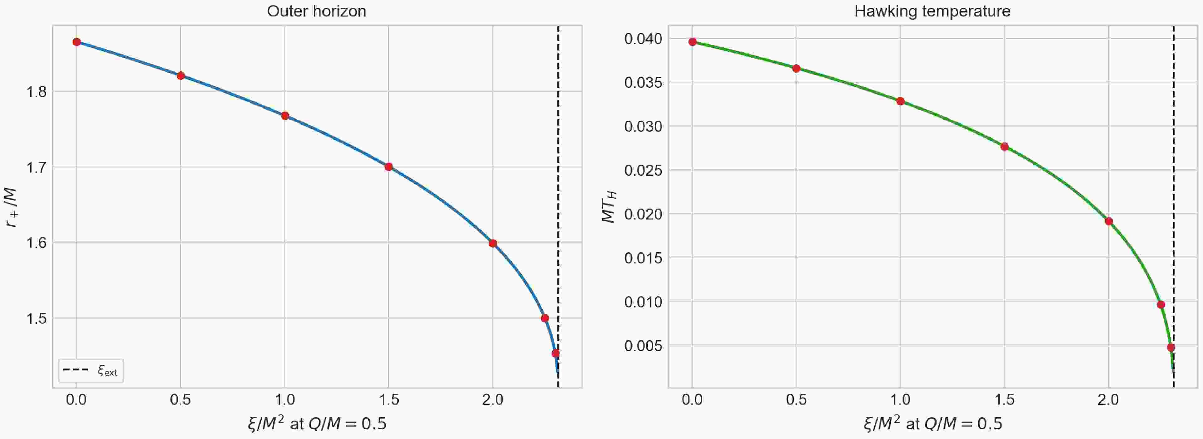
Table 1 lists the benchmark geometries. Figure 1 shows the full fixed-charge branch. As the non-minimal coupling approaches its extremal value, the outer horizon moves inward and the Hawking temperature decreases to zero. Figure 2 shows how the same parameter choices affect the metric function and the lowest effective barriers. This collapse of the temperature dominates the Hawking flux computed below.

Figure 1.  (color online) Outer horizon radius and Hawking temperature for the fixed-charge branch with $ Q/M=0.5 $. The dashed line indicates the extremal value of the non-minimal coupling.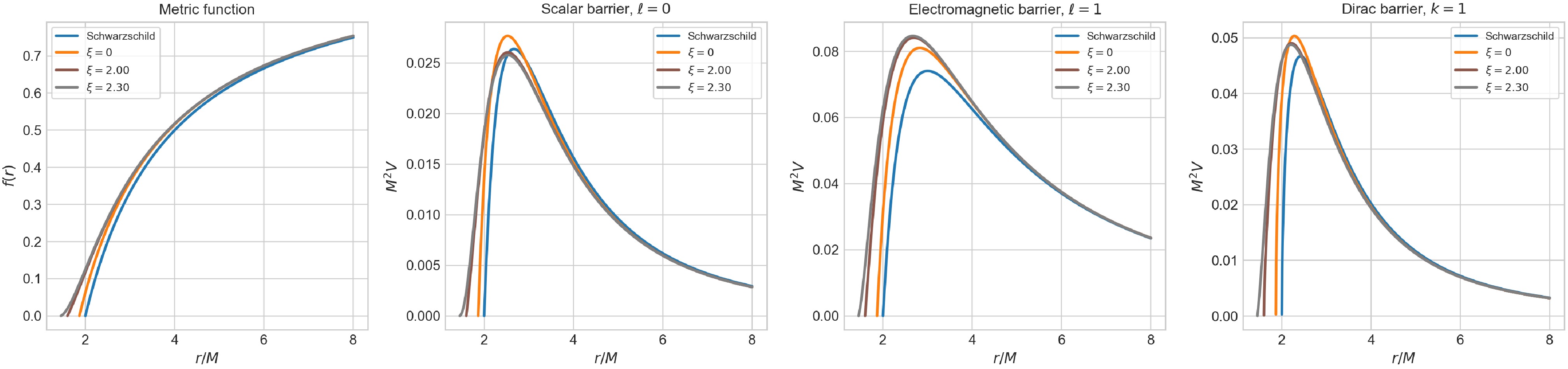

Figure 2.  (color online) Metric function and representative effective potentials for the Schwarzschild limit, the minimally coupled charged reference case, and two non-minimal Yang–Mills benchmarks. The plotted potentials correspond to the scalar $ \ell=0 $, electromagnetic $ \ell=1 $, and Dirac $ k=1 $ barriers.

The scattering calculation uses real frequencies ω and real transmission probabilities. This is different from the quasinormal-mode eigenvalue problem, where the boundary conditions are outgoing at infinity and the allowed frequencies are discrete and complex. The quasinormal-mode terminology appears only as motivation and as a reference to previous work on the same background.

Massless perturbations on a static, spherically symmetric background reduce to a Schrödinger-type equation in the tortoise coordinate.

Here, $ r_* $ is the tortoise coordinate, Ψ is the radial mode function, ω is the mode frequency, and $ V(r) $ is the spin-dependent effective potential. For a minimally coupled scalar field (see, for example, Refs. [31, 32]), we obtain

For electromagnetic test fields, the potential is given by (see Ref. [33] and the references therein)

For a massless Dirac field, we use the standard supersymmetric partner potential (see [34−38] and references therein for details),

Both chiral partner potentials yield the same transmission probability. We do not introduce a gravitational effective potential in the present analysis. The reason is not merely technical. In the present theory the background solves the coupled equations following from Eq. (1); therefore a metric perturbation $ h_{ik} $ changes not only $ G_{ik} $ but also $ T_{ik}^{\rm YM} $ and the non-minimal terms $ T_{ik}^{\rm NM} $, which contain explicit curvature couplings. Schematically, the linearized equation is

with the Yang–Mills perturbations and the curvature-dependent source varied consistently. A frozen-source Regge–Wheeler equation would set the right-hand side to zero while keeping a background supported precisely by that source. It would therefore describe an auxiliary test tensor field, not the physical graviton channel of the non-minimal Yang–Mills black hole. The fully coupled perturbation problem must be derived separately from the field equations of Refs. [27, 28].

The boundary conditions are purely ingoing waves at the event horizon and a superposition of incoming and outgoing plane waves at infinity.

The greybody factor is

The last expression assumes the standard normalization in which the ingoing horizon amplitude is unity. Numerically we solve the equation in the original radial coordinate, using

The integration starts at $ r_0=r_+(1+10^{-6}) $ with the Frobenius form of an ingoing wave, implemented as $ \Psi(r_0)=1 $ and ${\rm d}\Psi/{\rm d}r|_{r_0}=-{\rm i}\omega\Psi(r_0)/f(r_0)$. At a large extraction radius R the numerical solution and its tortoise derivative ${\rm d}\Psi/{\rm d}r_*=f\,{\rm d}\Psi/{\rm d}r$ are matched to the two plane waves in Eq. (18) by

Only the moduli of these quantities are needed, so the arbitrary additive constant in $ r_* $ drops out. The production runs used an adaptive high-order Runge–Kutta integration with relative and absolute tolerances at or below $ 10^{-9} $, extraction radii in the range $ R/M=400 $–$ 1200 $, and frequency refinement near each half-transmission point. Flux conservation was monitored through $ \left||A_{\rm in}|^2- |A_{\rm out}|^2-1\right| $. The largest residual in the data used for the figures and tables is below $ 4.5\times10^{-4} $, and representative reruns with $ R/M=400,800,1200 $ changed the dominant half-transmission frequencies by less than $ 2\times10^{-5} $ in $ M\omega $. The luminosity integrations were repeated after increasing the frequency range and the angular cutoff; the changes were smaller than the displayed precision in Table 2. These checks make the direct calculation a controlled convergent numerical procedure: as the tolerance, extraction radius, frequency grid and multipole cutoff are tightened, the greybody factors and integrated powers approach stable values.

The half-transmission tests above probe frequencies near the barrier top. To test the much lower frequencies that dominate the near-extremal Hawking integral, we performed an additional calculation with the extraction radius scaled to the wavelength. The production check uses relative and absolute tolerances $ 2\times10^{-9} $ and $ 2\times10^{-11} $ and $ R/M=\max(800,70/(M\omega)) $. In the tight rerun these are replaced by $ 2\times10^{-11} $, $ 2\times10^{-13} $ and $ R/M=\max(1400,120/(M\omega)) $, while the fractional horizon offset is reduced from $ 10^{-6} $ to $ 3\times10^{-7} $. The comparison covers $ 0.12\leqslant\omega/T_H\leqslant18 $ at $ \xi/M^2=2.30 $, including the full thermally relevant region shown in Fig. 3. This check is designed specifically for the regime $ \Gamma\ll1 $.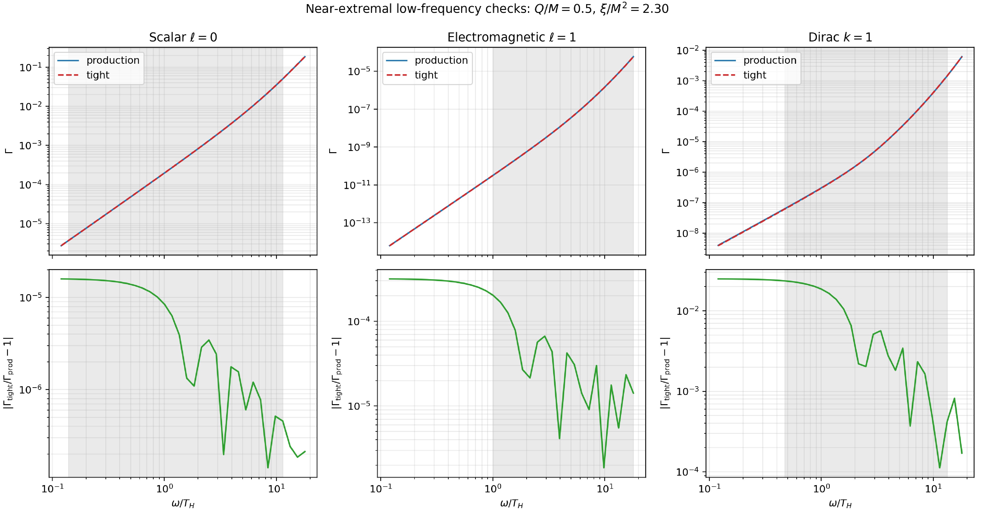

Figure 3.  (color online) Low-frequency greybody-factor convergence for the near-extremal benchmark with $ Q/M=0.5 $ and $ \xi/M^2=2.30 $. The upper panels compare the production and tight-grid calculations for the dominant scalar, electromagnetic, and Dirac modes as functions of $ \omega/T_H $. The lower panels show the corresponding relative differences. In each column, the shaded interval indicates the region where the corresponding tight-grid Hawking integrand is at least $ 1\ $% of its maximum.

As a barrier-top check, we also use WKB transmission formulae [39−43]. The WKB approach, particularly its higher-order extensions, has been used in numerous studies of black-hole scattering and quasinormal modes; see, e.g., Refs. [44−62] and references therein. It therefore provides a standard benchmark for greybody calculations. In the present work, WKB is not the primary data source. We use it for two limited purposes: first, to verify the expected agreement with direct integration as the multipole number increases, and second, to quantify the extent to which WKB can deviate for the low multipoles that dominate the Hawking flux. Because WKB estimates are frequently used for greybody factors, this comparison also serves as a cautionary test of their reliability for integrated radiation rates. The leading expression is shown only to fix notation:

where $ V_0 $ and $ V_0'' $ are evaluated at the maximum of the potential as a function of $ r_* $. At first order, the half-transmission condition is $ \Gamma_{\rm WKB1}=1/2 $, so the exponential equals unity and $ \omega_{1/2}^{\mathrm{WKB1}}=\sqrt{V_0} $. The WKB values quoted below, however, are obtained from the third-order Iyer–Will continuation rather than from this leading-order estimate. The third-order formula includes the standard higher-derivative barrier-top corrections and substantially reduces the leading-order barrier-top bias for the low multipoles considered here. Its half-transmission point is obtained by setting the continued-WKB parameter to $ \nu=0 $, which gives $ \Gamma_{\rm WKB3}=1/2 $. We quote WKB errors as fractional errors in the predicted half-transmission frequency,

Thus, the first-order expression used only as a guide is $ \delta_1=\sqrt{V_0}/\omega_{1/2}^{\mathrm{num}}-1 $, whereas Table 3 and Fig. 4 use $ N=3 $. Although WKB methods of various orders have been widely used in studies of greybody factors and quasinormal modes [29, 63−73], this method is an asymptotic barrier-top expansion rather than a convergent numerical scheme. Its optimal order and residual error generally cannot be predicted a priori; consequently, increasing the formal WKB order does not, by itself, guarantee a more accurate greybody factor. Therefore, we use direct numerical integration as the primary method for the Hawking-radiation calculations [2, 74, 75].

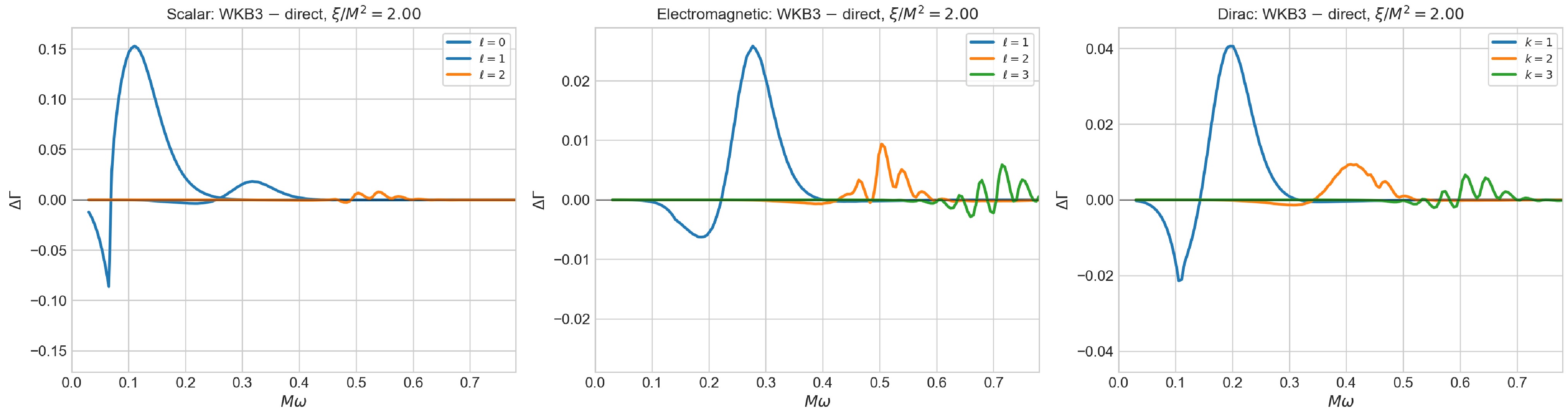
Figure 4.  (color online) Frequency-resolved WKB residuals are shown for the benchmark $ Q/M=0.5 $, $ \xi/M^2=2.00 $. Each panel shows $ \Delta\Gamma=\Gamma_{\rm WKB3}-\Gamma_{\rm num} $ for the first three scalar, electromagnetic, or Dirac modes as a function of the dimensionless frequency $ M\omega $. The residuals are plotted directly, rather than overlaid on the greybody factors, so that the sign and magnitude of the WKB deviation can be read as functions of frequency.

Figure 5 shows the direct-integration greybody factors. The dominant scalar threshold is lower than the electromagnetic threshold, as expected for the scalar monopole. Introducing the magnetic charge at $ \xi=0 $ shifts the barriers upward relative to the Schwarzschild case. Increasing the non-minimal coupling then changes the dominant thresholds only mildly: most half-transmission points drift upward by a few percent, whereas the scalar monopole and the lowest Dirac mode remain nearly unchanged. The chosen points are representative rather than observationally fitted. The value $ Q/M=0.5 $ is far enough from the neutral Schwarzschild limit to show charge effects, but sufficiently below the maximal charged regime that a broad interval in $ \xi/M^2 $ remains available before extremality. The sequence $ 0\leqslant\xi/M^2\leqslant2.30 $ then samples the minimally coupled charged case, intermediate non-minimal corrections, and a near-extremal point with $ \xi/\xi_{\rm ext}\simeq0.994 $. Since no phenomenological bound on this effective non-minimal Yang–Mills coupling is assumed in the present model, we do not exclude parameter values observationally; the only self-consistency restriction imposed here is the existence of the regular black-hole horizon, $ 0\leqslant\xi\leqslant\xi_{\rm ext} $ at the fixed value of $ Q/M $. The emitted test fields considered below are neutral with respect to the background Yang–Mills magnetic charge, so the instantaneous Hawking spectra describe radiation from fixed magnetic-charge backgrounds rather than discharge of the monopole. We use $ Q/M=0.5 $ as the central branch for the detailed greybody-factor analysis and include two bracketing charge branches in the integrated-power analysis: a weakly charged case, $ Q/M=0.1 $, and a strongly charged case close to the charged Reissner–Nordström limit, $ Q/M=0.9 $. Together these branches show how the luminosity suppression behaves from nearly neutral to strongly charged backgrounds.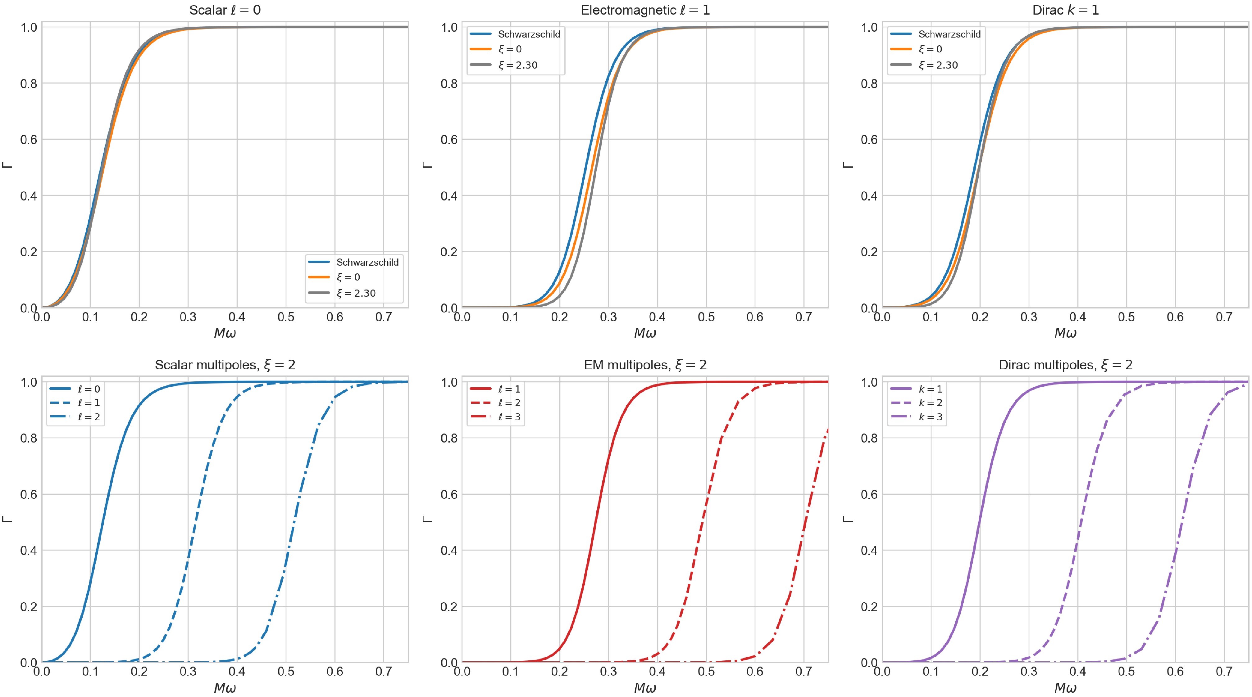

Figure 5.  (color online) Directly computed numerical greybody factors. The upper row compares the dominant modes for the Schwarzschild geometry, the minimally coupled charged reference case, and the near-extremal non-minimal geometry. The lower row shows the multipole hierarchy for $ Q/M=0.5 $ and $ \xi/M^2=2.0 $.

Table 4 lists the half-transmission frequencies. Here, $ \omega_{1/2}^{\rm num} $ denotes the real scattering frequency at which the direct numerical greybody factor satisfies $ \Gamma(\omega_{1/2}^{\rm num})=1/2 $. Along the fixed-charge branch, the dominant electromagnetic half-transmission point shifts from $ M\omega_{1/2}\simeq0.266 $ in the charged minimally coupled case to $ M\omega_{1/2}\simeq0.275 $ at $ \xi/M^2=2.30 $. The dominant Dirac point remains near $ M\omega_{1/2}\simeq0.20 $. These quantities characterize only the barrier-top region; alone, they do not determine how the greybody factors enter a near-extremal Hawking integral at $ \omega=O(T_H) $.

Figure 3 therefore examines the dominant modes directly on the thermal frequency scale for the most near-extremal benchmark. The upper panels show that the scalar, electromagnetic and Dirac transmission probabilities remain smooth down to very small values of Γ, while the lower panels compare the production and tight calculations throughout the shaded thermal-support intervals. This frequency-resolved test, rather than the modest displacement of $ \omega_{1/2} $, is the relevant numerical evidence for the low-frequency part of the power integral. Within the shaded intervals the largest production–tight relative differences are $ 1.6\times10^{-5} $ for the scalar mode, $ 2.0\times10^{-4} $ for the electromagnetic mode and $ 2.35\times10^{-2} $ for the Dirac mode. The corresponding production-run flux-balance residuals remain below $ 1.5\times10^{-10} $. The larger pointwise Dirac difference occurs at the low-frequency edge, where Γ is smallest; its effect on the integrated Dirac power is much smaller, as quantified below.

The third-order WKB comparison in Table 3 supports the same conclusion while avoiding the substantial leading-order barrier-top bias. The first-order estimate is useful analytically, but for the extended low-multipole table it overestimates the scalar monopole half-point by approximately 30 percent. The third-order continuation reduces the deviations for the electromagnetic and higher-multipole entries to the sub-percent or percent level, whereas the scalar monopole remains the channel least well described by WKB, with deviations of order ten percent. The relative WKB errors remain nearly constant as ξ approaches the extremal value, indicating that the barrier shape changes smoothly even as the temperature collapses. As a frequency-resolved diagnostic, we plot the residual $ \Delta\Gamma=\Gamma_{\rm WKB3}-\Gamma_{\rm num} $ as a function of frequency. A sixth-order continuation was tested for the same low modes, but it was not uniformly more stable for this non-minimal Yang–Mills sequence. Therefore, Fig. 4 and Table 3 use the cleaner third-order continuation.

In this comparison, the direct numerical integration should be regarded as the reference result. It solves the radial scattering equation with the imposed ingoing horizon boundary condition and checks flux conservation at infinity; thus, its remaining uncertainty is controlled by the integration tolerance, extraction radius, and quoted flux-balance residual. The WKB values have a different status: they are obtained from a local expansion around the maximum of the effective potential and form an asymptotic, not necessarily convergent, series. Therefore, increasing the formal WKB order does not guarantee a smaller error for low multipoles or away from the barrier top. The residuals in Fig. 4 should consequently be interpreted primarily as the frequency-dependent WKB approximation error relative to the numerical greybody factors.

The pattern in Table 3 illustrates the two intended uses of the WKB calculation. For increasing multipole number the agreement with direct integration rapidly improves, which is the expected eikonal trend and serves as an additional check on the potentials and numerics. At the same time, the scalar monopole and the lowest Dirac and electromagnetic modes show that WKB errors are not negligible precisely in the channels that carry much of the Hawking flux. The integrated powers in Table 2 are therefore based on the controlled direct greybody factors, not on WKB estimates alone.

The preceding section establishes that the exterior transmission probabilities vary smoothly along the fixed-charge branch. The next step is to fold those probabilities with the thermal occupation numbers. This is where the falling surface gravity enters directly, so the comparison between greybody thresholds and luminosity becomes quantitative.

The energy spectrum at infinity is computed within the quasi-stationary approximation. The black hole is assumed to change negligibly during the emission of individual quanta; in particular, the Hawking temperature is taken to be identical for two consecutively emitted particles at a fixed point in the benchmark sequence. The temperature changes only when transitioning to a different background in the parameter sequence. With this assumption,

where j labels the field and angular mode, $ g_j $ is the corresponding degeneracy, and the minus (plus) sign applies to bosons (fermions). The degeneracy factors are $ 2\ell+1 $ for scalar modes, $ 2(2\ell+1) $ for electromagnetic modes, and $ 2k $ for massless two-helicity Dirac modes. The integrated powers are obtained from $P=\displaystyle\int_0^\infty({\rm d}^2E/{\rm d}t\,{\rm d}\omega){\rm d}\omega$. In Table 2, $ P_S $ denotes this total for one real scalar field, $ P_\gamma $ denotes the total for one Maxwell field after summing over the electromagnetic multipoles, and $ P_D $ denotes the total for one massless two-helicity Dirac species after summing over the Dirac modes. The photon-plus-light-fermion proxy used below is $ P_\gamma+3P_D $, following the same normalization convention as in the Page comparison. This is a deliberately restricted massless-field proxy, not a calculation of the full Standard Model emission. In Page’s four-dimensional Schwarzschild benchmark, photons plus three light Dirac species already carry about $ 98\ $% of the combined photon–light-fermion–graviton luminosity [2]. The proxy is therefore useful for comparing the selected channels across the black-hole branch, but no claim is made here regarding massive charged fermions, non-Abelian gauge bosons, or other particle thresholds.

Table 2 gives the integrated powers. The minimally coupled charged reference already emits less than the Schwarzschild case in the photon-plus-light-fermion proxy. Increasing the non-minimal coupling then rapidly suppresses the luminosity: for the fixed-charge sequence, the proxy is approximately one-half of the Schwarzschild value at $ \xi/M^2=0.50 $, approximately one-quarter at $ \xi/M^2=1.00 $, below one percent at $ \xi/M^2=2.00 $, and below one millionth at $ \xi/M^2=2.30 $. The origin of this suppression is tested below by varying the temperature and the greybody factors separately. To separate cooling from the change of the transmission probabilities, let $ P[T,\Gamma] $ denote the power obtained by inserting a specified temperature and set of greybody factors into Eq. (24). With the charged minimally coupled geometry, $ Q/M=0.5 $ and $ \xi=0 $, as the reference, we evaluate

Thus $ P_T $ changes only the thermal occupation factor, whereas $ P_\Gamma $ changes only the scattering input. This comparison uses the complete frequency-dependent greybody factors in the integral and does not rely on $ \omega_{1/2} $ as a proxy. The charge dependence of the integrated powers is displayed in Table 5. Since the extremal value of $ \xi/M^2 $ depends strongly on $ Q/M $, the rows are labelled by the fraction $ \xi/\xi_{\rm ext}(Q/M) $ as well as by the actual value of $ \xi/M^2 $. The weak-charge branch stays close to Schwarzschild at $ \xi=0 $, whereas the high-charge branch is already cooler and dimmer in the minimally coupled limit. On both branches, however, moving toward the non-minimal extremal surface suppresses $ P_\gamma+3P_D $ by many orders of magnitude. Thus a strong luminosity quench is common to the weak, intermediate and strongly charged branches considered here; the explicit temperature–greybody decomposition in Table 6 is made for the central $ Q/M=0.5 $ branch.

Table 7 shows that the largest production–tight change in an integrated power is $ 1.04\times10^{-3} $, while the multipole tail is far smaller. The revised last two rows of Table 2 differ by at most $ 2.7\ $% from the values in the preceding manuscript version, which used the finite-radius setup optimized around the barrier region. To include that independent shift as well as the much smaller strict-rerun variation, we conservatively assign a $ 3\ $% relative numerical uncertainty to the $ \xi/M^2=2.25 $ and $ 2.30 $ powers. This uncertainty is negligible compared with their many-orders-of-magnitude suppression.

The control calculation in Table 6 gives a more precise interpretation of the mechanism. At $ \xi/M^2=2.30 $, cooling alone reduces the proxy to $ 1.94\times10^{-5} $ of the charged minimally coupled value, whereas changing the greybody factors alone at the reference temperature gives $ 0.835 $ of that value. When both effects are included, the ratio is $ 9.13\times10^{-7} $: the altered low-frequency greybody factors provide a further factor of about $ 21 $ beyond the cooling-only result. Thus cooling accounts for the largest number of suppressed orders of magnitude, but the low-frequency transmission change is not negligible close to extremality. The same pattern, with smaller additional greybody factors of about $ 1.8 $ and $ 5.6 $, occurs at $ \xi/M^2=2.00 $ and $ 2.25 $.

Figure 6 shows the spectra. Although the dominant greybody thresholds vary only slightly, the spectra are strongly suppressed as the extremal coupling is approached. The peak frequencies also shift to lower values because the thermal scale is set by the decreasing Hawking temperature. This effect is strongest for bosonic channels with higher thresholds, whereas the Dirac channel remains comparatively more important near the endpoint.

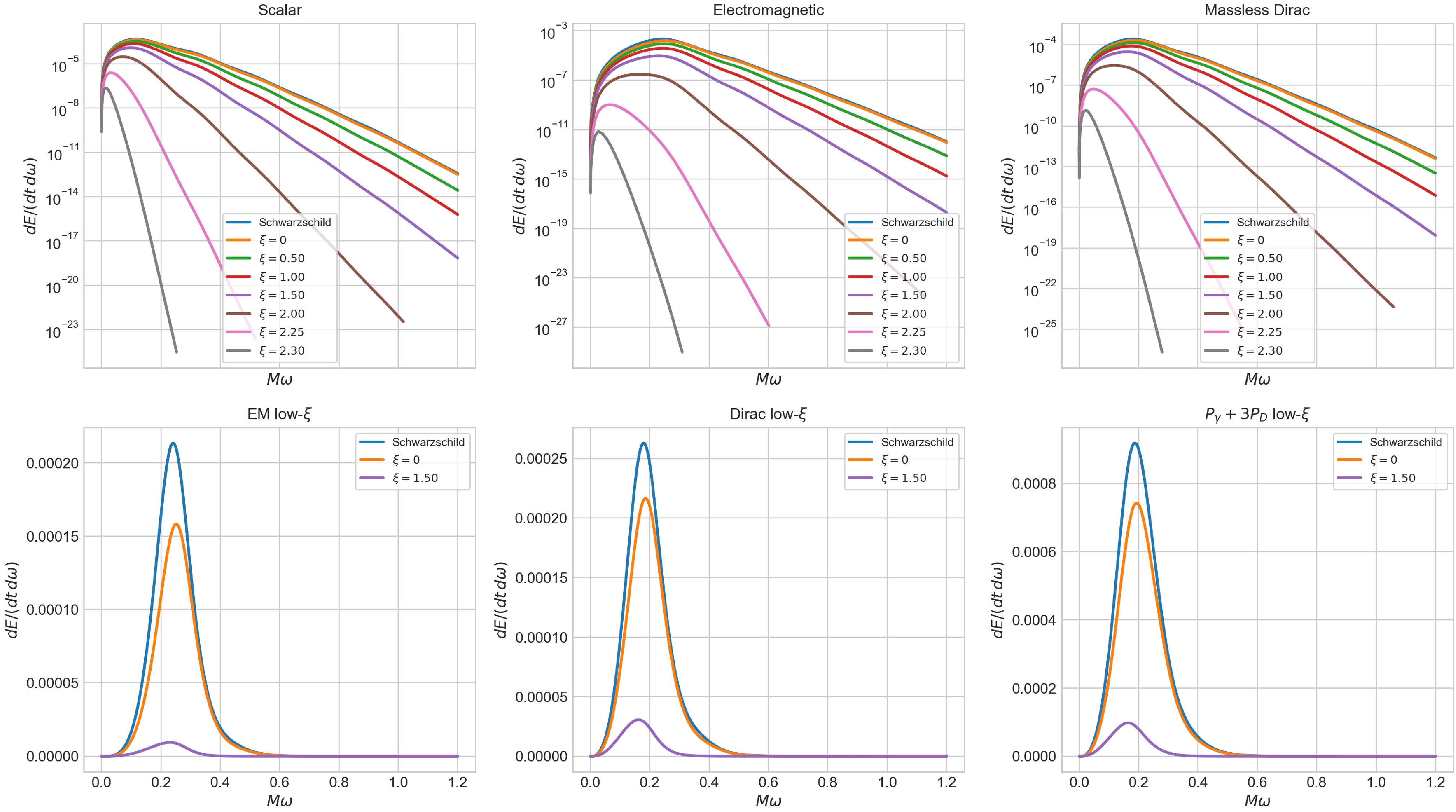
Figure 6.  (color online) Hawking energy-emission spectra in mass-scaled units. The horizontal axis is $ M\omega $, and the plotted spectra are the corresponding dimensionless powers per dimensionless frequency interval. The upper row presents logarithmic spectra for scalar, photon, and massless Dirac channels. The lower row shows representative low-coupling photon, Dirac, and photon-plus-three-Dirac proxy spectra.

The relative composition of the flux also changes. For the Schwarzschild case and the minimally coupled charged reference, the photon and Dirac contributions are comparable in the Page proxy. Near the non-minimal extremal endpoint, however, the photon channel is suppressed much more efficiently than the Dirac channel. In the final benchmark row, the Dirac contribution dominates the photon-plus-light-fermion proxy. This is the same qualitative pattern expected whenever the thermal scale falls below the dominant bosonic barrier threshold.

The luminosities in the previous section are instantaneous equilibrium rates. They should not be confused with an evaporation trajectory until one specifies how the parameters of the black-hole solution evolve. We therefore separate the robust local result, namely the {strong near-extremal luminosity suppression}, from the more model-dependent question of the total lifetime.

The fixed-mass calculations above compare different members of the black-hole family at the same ADM mass. A physical evaporation history requires an additional prescription for the evolution of the magnetic Yang–Mills charge and the non-minimal coupling. If both are held fixed as dimensional quantities, the dimensionless ratios $ Q/M $ and $ \xi/M^2 $ increase as the mass decreases, driving the black hole toward an extremal surface in the two-parameter space. If charge is emitted or screened, the trajectory may differ. Because non-Abelian charge loss and the possible running of non-minimal couplings are model dependent, we do not assign a unique lifetime in this first study.

Nevertheless, the fixed-mass sequence provides a robust local result. Along a path of increasing non-minimal coupling at fixed magnetic charge, the greybody factors remain smooth, while the Hawking temperature tends to zero. Therefore, any adiabatic trajectory that approaches the cold extremal surface without a compensating increase in charge loss will undergo strong luminosity suppression. The finite powers in Table 2 should be interpreted as instantaneous equilibrium luminosities, not as a complete backreacting evaporation model.

There are also perturbative limitations. The scalar, electromagnetic, and Dirac sectors are treated as test fields on the fixed background. We deliberately do not quote graviton emission rates: a complete gravitational calculation would require the coupled perturbations of the metric and the non-minimally coupled Yang–Mills source, including the right-hand side of the perturbed Einstein equations. Massive particle thresholds are also neglected, so the photon-plus-light-fermion proxy is meaningful only for species whose rest masses are small compared with the instantaneous Hawking temperature.

No greybody-factor–quasinormal-mode correspondence is assumed in deriving these results. The earlier scalar quasinormal-mode study is used only to identify a relevant background and scalar channel; our numerical input for the Hawking spectra is the real-frequency scattering problem described above.

We computed greybody factors by direct integration and quasi-stationary Hawking emission rates for the regular non-minimal Einstein–Yang–Mills black hole. The background is controlled by the magnetic Yang–Mills charge Q and the non-minimal curvature-coupling parameter ξ. For the representative branch $ Q/M=0.5 $, the black hole approaches an extremal endpoint at $ \xi/M^2= 2.313766198591 $, where the Hawking temperature vanishes.

The direct-integration results show that the greybody thresholds are comparatively insensitive to the non-minimal coupling. The dominant electromagnetic and Dirac half-transmission frequencies vary only mildly between the minimally coupled charged reference and the near-extremal non-minimal geometry. Third-order WKB estimates, used here as a standard barrier-top benchmark rather than as reference data, confirm that the barrier structure evolves smoothly. They also explain why WKB alone is not sufficiently reliable for accurate Hawking-power estimates in the dominant low-multipole channels, even though it reproduces the higher-multipole trend well. The new thermal-window calculation demonstrates that the half-transmission points do not provide the full picture: at $ \xi/M^2=2.30 $, cooling alone suppresses the photon-plus-three-Dirac proxy by a factor of approximately $ 5.2\times10^4 $, while the modified low-frequency greybody factors provide an additional factor of approximately $ 21 $. Cooling is therefore the dominant source of the total orders-of-magnitude reduction on the branches studied here, but the greybody contribution is not negligible near extremality.

The integrated luminosities decrease rapidly as the extremal endpoint is approached. For the photon-plus-three-Dirac proxy, the fixed-charge sequence decreases from approximately eighty percent of the Schwarzschild value in the minimally coupled charged reference to less than one percent at $ \xi/M^2=2.00 $ and to less than one millionth at $ \xi/M^2=2.30 $. The residual massless particle flux becomes increasingly dominated by fermions. Across the charge branches the same strong suppression persists. At $ Q/M=0.1 $ the minimally coupled row is essentially Schwarzschild-like, but the proxy luminosity falls to $ 4.3\times10^{-3} $ and then $ 4.7\times10^{-6} $ of the Schwarzschild value at $ 0.90\xi_{\rm ext} $ and $ 0.99\xi_{\rm ext} $. At $ Q/M=0.9 $ the charged geometry is already dimmer at $ \xi=0 $, and the corresponding ratios fall to $ 2.6\times10^{-4} $ and $ 2.5\times10^{-7} $. The detailed division between temperature and greybody effects may depend on the charge branch and is quantified here only for $ Q/M=0.5 $.

Recent studies have suggested that greybody factors and quasinormal modes can be related through the common effective potential governing wave propagation. In that approach, the scattering coefficients for transmission through and reflection from the potential barrier may encode information about the resonant spectrum of the system [76, 77]. Scattering data can therefore provide a complementary route for probing quasinormal spectra, alongside traditional frequency-domain and time-domain analyses of black-hole perturbations [78−82]. We emphasize, however, that this correspondence is not used as an input in the present Hawking-emission calculation. Our greybody factors are obtained from the real-frequency scattering problem, and a future comparison with the quasinormal spectrum of the same Einstein–Yang–Mills background would be a separate test. Such a test is worthwhile precisely because the correspondence is not guaranteed for arbitrary potential shapes [83−85].

Future work should extend this calculation in three directions: by developing a fully coupled gravitational perturbation theory for the non-minimal Yang–Mills source, incorporating massive-particle thresholds and charge-emission channels, and constructing a dynamical evaporation model in which M, Q, and the effective non-minimal coupling evolve self-consistently. The instantaneous powers computed here assume that the temperature remains unchanged between consecutive emissions; therefore, they should be used as local inputs to such an evaporation model rather than as a complete lifetime calculation. For the branches and neutral test fields considered here, approaching the regular extremal endpoint suppresses Hawking radiation predominantly through horizon cooling, with an increasingly important additional correction from the low-frequency Maxwell and Dirac greybody factors.