Machine-Learning-Based prediction of heavy-ion capture cross sections with system-level cross-validation

In nuclear physics research, the capture cross section of heavy-ion capture reactions is regarded as a crucial observable for understanding the dynamics of nuclear interactions [1−6]. Its accurate description is not only of fundamental importance for exploring non-equilibrium dynamical processes in quantum many-body systems but also provides an indispensable theoretical basis for the synthesis pathways of superheavy elements [7−10]. Furthermore, in astrophysical environments [11−14], the production rates of key nuclides are directly and significantly influenced by capture cross sections in the relevant energy regions. Consequently, as a bridge connecting microscopic nuclear structure with macroscopic reaction phenomena, the systematic study of capture cross sections continuously promotes the coordinated development of nuclear reaction theory and nuclear technology applications.

In recent years, systematic progress has been achieved in both theoretical and experimental studies of heavy-ion capture cross sections [15−17]. Existing theoretical models, such as the modified empirical barrier distribution (EBD) model [18], the coupled-channels (CC) model [19, 20], the empirical coupled-channel (ECC) model [21, 22], and the Wong formula [23], are generally capable of reproducing experimental cross sections well in the near-barrier energy region. Meanwhile, the development of the time-dependent Hartree-Fock method [24−26] has enabled the prediction of capture cross sections without empirical parameters, significantly enhancing the self-consistency and predictive power of theoretical models. Furthermore, an important theoretical advance is the proposal of a new energy and cross section scaling method [27], which eliminates the influence of the Coulomb barrier and enables data from different heavy-ion fusion systems to be compared on the same universal curve.

Experimentally, continuous improvements in detection techniques and beam quality have enabled precise measurements in the deep sub-barrier energy region, clearly revealing fusion hindrance [28, 29]. Experiments using radioactive beams have directly observed the influence of loosely bound valence nucleons on cross sections, offering key insights into the fusion dynamics of halo and weakly bound systems [30, 31]. Together, these experimental and theoretical efforts complement each other and advance capture cross-section research toward greater accuracy and consistency.

However, the theoretical description of capture cross sections has long faced several major challenges. This difficulty primarily stems from the fact that the fusion process itself is an extremely complex quantum many-body dynamical problem [32, 33], involving strong coupling effects between nuclear structural degrees of freedom and relative motion. Moreover, substantial limitations persist in the ability of traditional theoretical models to accurately describe the complex dependence of sub-barrier fusion cross sections [34, 35] on entrance-channel properties [36], such as mass asymmetry and neutron asymmetry. In particular, when the sign of the reaction Q-value changes [31, 37], the models often lack sufficient precision in characterizing cross-section enhancement effects. Furthermore, their generalization capability to unmeasured projectile-target combinations remains limited, hindering their predictive capacity in frontier research areas such as superheavy element synthesis and astrophysics.

Over the past decade, machine learning methods have been extensively and successfully applied to data analysis in various branches of physics. In nuclear physics, they have been employed to predict a wide range of nuclear observables. These include ground-state properties such as atomic masses [38−40] and binding energies [41], radioactive decay features including β-decay and α-decay half-lives and energies [42−44], as well as theoretical constructs and reaction channels such as the nuclear energy density functional [45] and evaporation residue cross sections [46].

As machine learning techniques continue to advance rapidly, novel approaches have emerged that further enhance predictive capabilities. Among them, Tabular Prior-data Fitted Network (TabPFN) [47] stands out as a recent innovation that enables physicists to obtain accurate predictions rapidly, offering a distinct advantage for analyzing the small-sample data frequently encountered in nuclear physics. In this paper, in addition to TabPFN, we adopt two other machine learning methods, Gaussian Process Regression (GPR) [48] and Backpropagation Neural Network (BP) [49], to achieve predictions that align more closely with experimental capture cross-section values. These three methods are trained and tested on capture cross sections from 566 projectile-target combinations, enabling comprehensive and accurate calculations of capture cross sections for nuclear reactions across systems ranging from light to superheavy nuclei. To thoroughly assess generalization capability, we employ two distinct data-splitting strategies: a point-wise random split (denoted by subscript P) and a system-wise split based on projectile-target combinations (denoted by subscript S), both with a training-to-test ratio of 8:2. Accordingly, each of the three models yields two variants, resulting in a total of six trained models.

Very recently, Bhat et al. [50] reported a machine-learning study on heavy-ion capture cross-section prediction, which also constructed physically motivated entrance-channel features and adopted Gaussian-process-based uncertainty estimation. Nevertheless, all performance evaluations in their work rely exclusively on the point-wise random-split protocol, in which different energy points belonging to the same projectile-target excitation function can appear in both the training and test partitions. Such an evaluation setup mainly probes interpolation performance for already-seen reaction systems. In contrast, the present work emphasizes system-level generalization assessment. We adopt both a system-wise 8:2 split and rigorous leave-one-system-out cross-validation (LOSO-CV), in which entire projectile-target pairs are fully held out for testing without leaking any energy information from the test system into the training set. This protocol enables a quantitative investigation of model performance for fully unseen projectile-target combinations, which constitutes the central novelty of our study.

The article is organized as follows. In Sec. II, we give a brief description of the theoretical framework. Results and discussion are presented in Sec. III. A summary is given in Sec. IV.

This section briefly introduces the three machine learning methods employed in the calculations and the dataset partitioning strategy.

Tabular Prior-data Fitted Network (TabPFN) is designed specifically for tabular-data classification and regression tasks. Based on the principle of in-context learning, this neural network uses a Bayesian inference mechanism in which pre-training on large synthetic datasets enables Bayesian prior knowledge to be internalized in the model parameters [47]. When applied to new real-world datasets, the method performs approximate Bayesian inference in a single forward pass, substantially reducing training time. The robustness of TabPFN is attributed to its pre-training process on extensive synthetic data. In its native design, TabPFN can filter irrelevant features and autonomously handle missing-value entries. In the present work, however, all samples with missing derived physical features are excluded during dataset cleaning; therefore, the native missing-value-handling capability of TabPFN is not invoked in our inference pipeline.

In our application, TabPFN uses the 13 input features described in Sec. II.D to predict the logarithmically transformed capture cross section. It outputs both the predictive mean and the lower and upper bounds of the prediction interval, which quantify uncertainty and provide the prediction intervals shown in Appendix A. TabPFN is pre-trained on a large corpus of synthetic datasets generated via structural causal model priors, allowing the model to acquire general priors for tabular regression tasks. Once applied to our dataset, it performs inference in a single forward pass without iterative optimization.

For reproducibility, the exact software configuration of TabPFN is documented here, following the original TabPFN publication [47]. We adopt the official open-source TabPFN v2 regression model together with its native pre-trained regression checkpoint tabpfn-v2-regressor.ckpt from the original publication [47]. This checkpoint is pre-trained on approximately $ 1.3\times 10^{8} $ synthetic tabular datasets generated primarily via structural-causal-model priors, consistent with the description in the original Nature work. No additional fine-tuning of the TabPFN neural-network weights is performed using our heavy-ion capture-cross-section dataset; all predictions are obtained solely through the in-context-learning paradigm with a single forward pass.

Instead of merely outputting a scalar point prediction, TabPFN regression natively yields a piecewise-constant probability distribution for the target variable. Following the native regression setup of the model, the boundaries of the predictive distribution are determined from the 1/5000 quantiles of the pre-training target distribution. All inference hyperparameters retain the official default configuration, with softmax temperature $ T=0.9 $. Neither temperature rescaling nor post-hoc variance recalibration is applied to the present dataset.

The nominal $ 95 $% prediction interval adopted in this work is constructed directly from this native model output. The reported $ 95 $% prediction interval is extracted by taking the $ 2.5 $% and $ 97.5 $% quantiles from the native forward-pass predictive distribution. No post-hoc correction or recalibration of prediction intervals is performed using ground-truth test-set values. We explicitly note that these are nominal model-generated prediction intervals, and we do not claim that they are empirically well calibrated for held-out unseen projectile-target test systems. Rigorous empirical coverage calibration is left for future research.

Gaussian Process Regression (GPR) is a nonparametric Bayesian method that defines a prior distribution over functions through a kernel function that measures similarity between samples [48]. In nuclear physics research, GPR provides an innovative methodology for predicting capture cross sections. A probabilistic model describing the evolution of cross sections with incident energy can be constructed from limited experimental observations, while reliable confidence intervals are generated simultaneously. By selecting appropriate kernel functions (such as the squared exponential or Matérn kernels), resonance-peak characteristics and smoothly varying regions in cross-section curves can be accurately captured. Consequently, this technique has significant applicability in multiple domains, including nuclear database compilation, theoretical model validation, and experimental design optimization. For a new input point $ x_* $, the predictive mean and variance are given by:

where K denotes the kernel matrix of the training samples, $ k(x_*) $ is the kernel vector between the test point and all training points, $ \sigma_n^2 $ represents the noise variance, and y is the target observation vector.

In this study, we employ the Matérn $ 5/2 $ kernel, which provides a favorable balance between smoothness and flexibility for describing capture cross-section excitation functions. The kernel hyperparameters and noise variance are optimized by maximizing the log-marginal likelihood. The training dataset is used to construct the kernel matrix K, and predictions at unobserved energy points are computed using Eqs. (1) and (2). This framework yields both point estimates and corresponding uncertainty bounds (confidence intervals) for capture cross sections.

A backpropagation neural network (BP) learns a mapping from input features to target values through iterative forward and backward propagation [49]. During the forward pass, the input x is transformed into a prediction.

where W denotes the weight matrix, b is the bias vector, and $ {\cal{F}} $ represents the activation function. The weights are updated using gradient descent to minimize the loss function.

In our implementation, the network architecture consists of an input layer, two hidden layers, and an output layer. The input layer contains 13 neurons corresponding to the selected input features. The two hidden layers contain 64 and 32 neurons, respectively, and both use the ReLU activation function. The output layer contains a single neuron with linear activation for regression tasks, which outputs the logarithmically transformed capture cross section $ \log_{10}\sigma_{\text{pred}} $.

The dataset used in this study comprises 566 projectile–target combinations, with a total of 14 465 experimental data points. A complete machine-readable metadata list covering all 566 projectile–target pairs, including the reaction label, number of experimental data points, experimental references, and cross-section units for each system, is provided in the Supplementary Material. To examine model performance under different generalization conditions, we employ two distinct data-splitting strategies: a random point-wise split (denoted by subscript P) and a system-wise split based on projectile–target combinations (denoted by subscript S), both with a training-to-test ratio of approximately 8:2. For each of the three machine learning methods (TabPFN, GPR, and BP), we train two variants under these strategies, resulting in a total of six trained models.

Previous studies [51] have shown that incorporating physical quantities related to the physical model as inputs for machine learning significantly improves accuracy compared with results obtained without such inputs. In this study, we use 13 input features: the proton numbers and mass numbers of the projectile and target nuclei ($ Z_{P} $, $ Z_{T} $, $ A_{P} $, $ A_{T} $), the center-of-mass energy ($ E_\text{c.m.} $), the quadrupole and hexadecapole deformation parameters of the projectile and target nuclei, the proton number, mass number, and binding energy of the compound nucleus, and the Bass barrier.

The nuclear quadrupole and hexadecapole deformation parameters, as well as the compound-nucleus binding energies, are extracted from the FRDM-95 nuclear mass table. The Bass fusion barrier height for each projectile–target pair is calculated using a publicly available Excel-based calculation tool widely used in heavy-ion fusion studies. This Excel calculator file is provided as part of the Supplementary Material to enhance reproducibility.

In this study, a logarithmic transformation was applied to the capture cross-section values to compress their large dynamic range [52]. The MAE was used as the metric for comparing the performance of the three machine learning models.

Here, N denotes the total number of data points in the training or test set, and $ \sigma_{\mathrm{pred}} $ and $ \sigma_{\mathrm{Exp.}} $ denote the predicted and experimental capture cross sections, respectively.

The MAEs of the training and test sets for the three machine learning models under the two data-splitting strategies are shown in Table 1, where the subscripts P and S denote the point-wise random split and the system-wise split based on projectile-target combinations, respectively. Under the point-wise split (P), $ \mathrm{TabPFN_P} $ achieves the lowest test MAE (0.0720), followed by $ \mathrm{GPR_P} $ (0.0846) and $ \mathrm{BP_P} $ (0.1533), confirming its superior interpolation capability within known systems. Under the system-wise split (S), which evaluates extrapolation performance for entirely unseen projectile-target combinations, all models exhibit markedly larger test errors. Notably, $ \mathrm{TabPFN_S} $ still yields the smallest test MAE (0.1981), $ \mathrm{BP_S} $ is intermediate (0.2505), whereas $ \mathrm{GPR_S} $ produces the largest error (0.7806). This indicates that the system-wise split constitutes a far more challenging evaluation scenario. The substantial performance degradation of $ \mathrm{\mathit{\mathrm{\mathit{GPR}}}_S} $ originates mainly from limitations of the kernel function: the fixed Matérn 5/2 kernel cannot adequately capture the strong nonlinear behavior for entirely unseen projectile-target pairs.

The distinct performance gaps among the six variants can be attributed to their inherent architectures. TabPFN, pretrained on massive synthetic tabular datasets, inherits informative Bayesian priors that enable efficient one-shot inference, making it resilient to both random data partitioning and systematic extrapolation. The BP network yields moderate errors but is sensitive to hyperparameter tuning and struggles to capture subtle sub-barrier coupling effects when experimental samples are limited. GPR, despite its flexibility, relies on a fixed Matérn 5/2 kernel, which fails to represent the strong nonlinearities (e.g., fusion hindrance and exponential fall-off) in the deep sub-barrier region. This deficiency is substantially amplified in the system-wise split, where the kernel cannot generalize to unknown projectile-target combinations, resulting in the highest test error among all models.

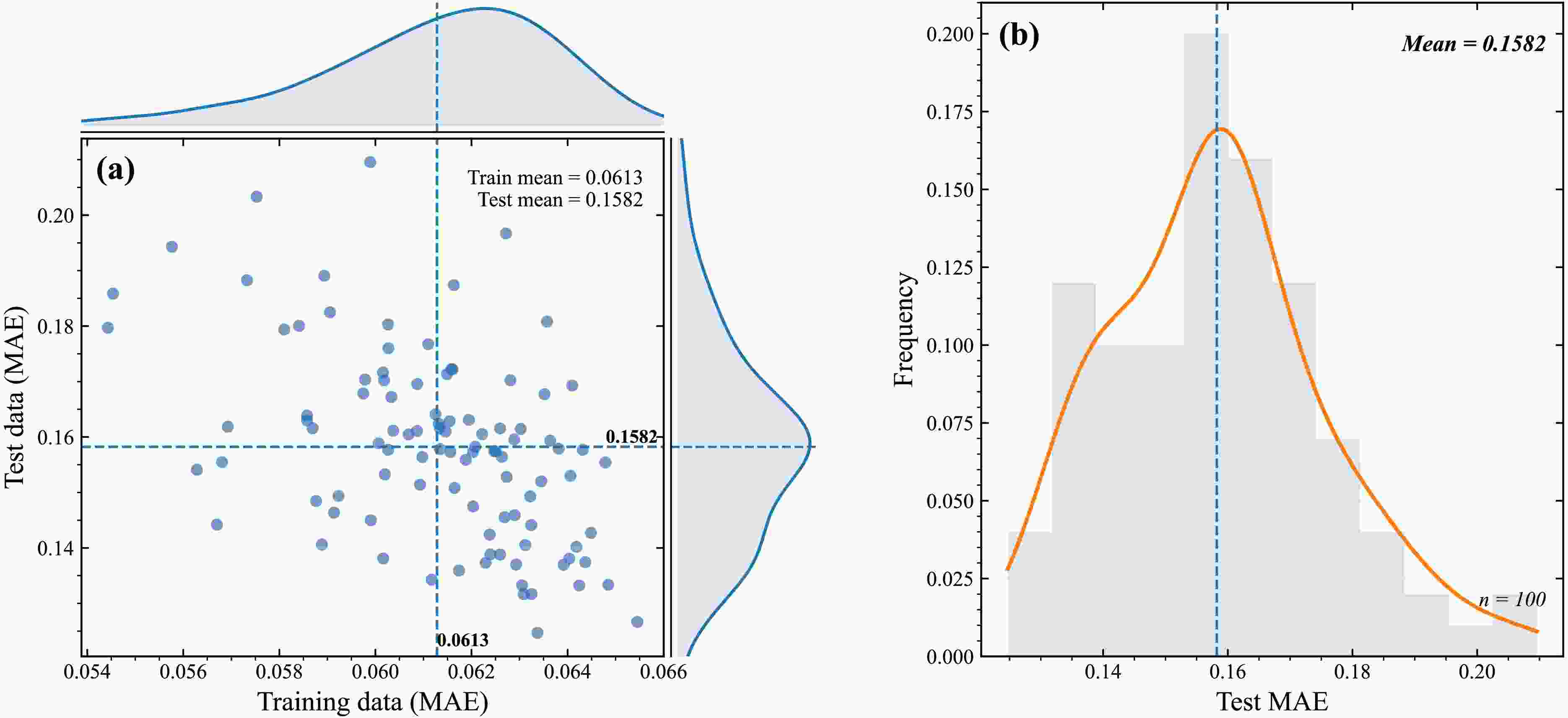
To rule out the possibility that the superior extrapolation performance of TabPFN_S arises from an accidental choice of the training-test split, we repeated the model training 100 times using different random seeds (1–100) while keeping the 8:2 partitioning ratio under the system-wise split scheme. In each repetition, random partitioning was performed over complete projectile-target combinations rather than over individual energy data points. The resulting distribution of MAE values is shown in Fig. 1. As shown in Fig. 1(a), the training MAE values are tightly concentrated around a mean of 0.0613, and the test MAE values are clustered around a mean of 0.1582, with moderate scatter. Figure 1(b) further confirms this stability, displaying a narrow unimodal histogram together with a kernel-density curve for the test MAE (mean = 0.1582, $ n=100 $). Notably, the result obtained with the single seed (seed 42) adopted in our main-text analysis lies very close to the overall average of the 100 repetitions, indicating that the reported performance is representative and not an outlier. These observations demonstrate that TabPFN_S is insensitive to the specific random partition, thereby reinforcing the reliability of its advantage over the other models.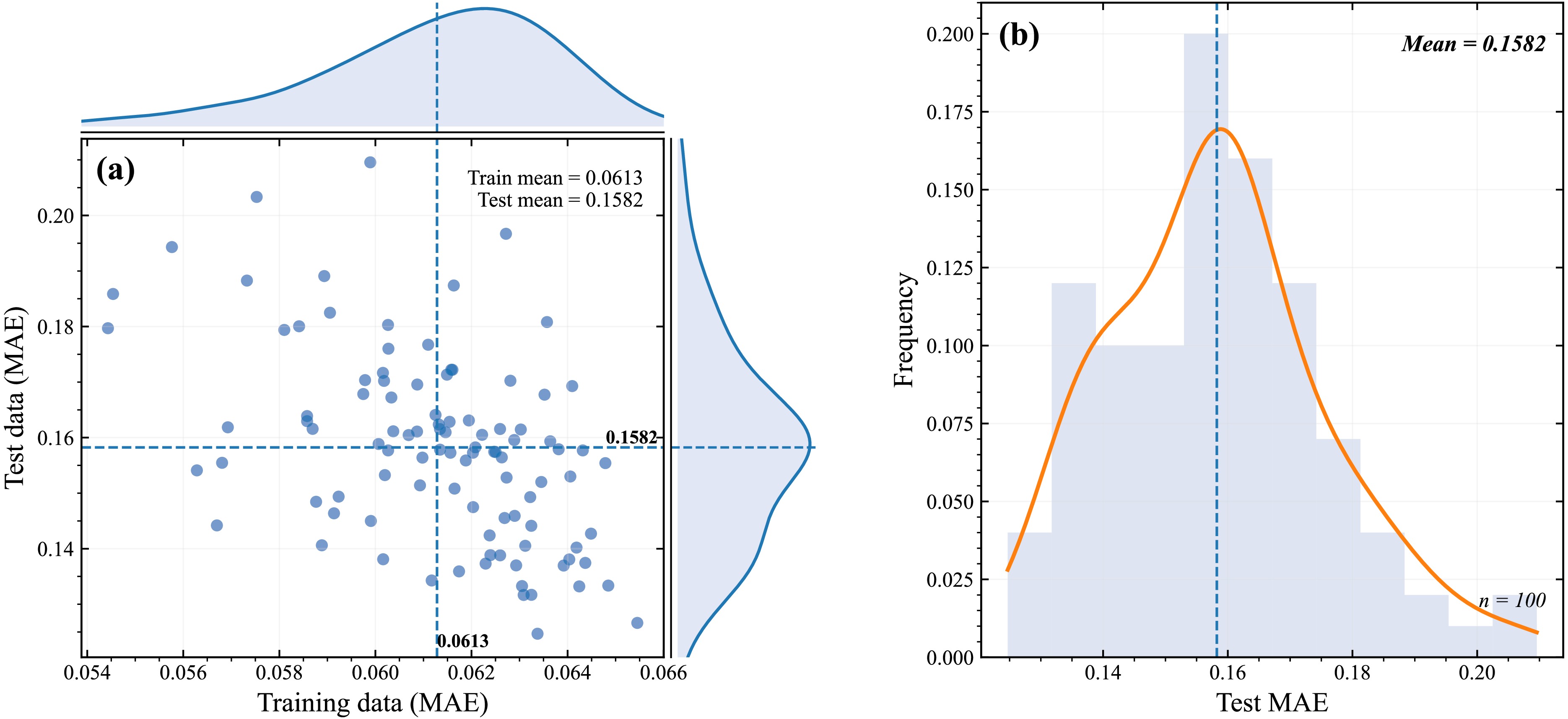

Figure 1.  (color online) Performance stability of TabPFN_S across 100 independent random train–test splits under the system-wise splitting scheme with an 8:2 training-to-test ratio. (a) Scatter plot of training-set MAE versus test-set MAE for 100 independent runs with random seeds from 1 to 100. Each random split partitions complete projectile–target combinations at the system level rather than shuffling individual energy points. The top and right margins show marginal kernel-density estimates for the training and test MAE, respectively. The blue dashed lines indicate the overall mean values (training mean = 0.0613; test mean = 0.1582). (b) Histogram with a kernel-density curve showing the frequency distribution of the test-set MAE across the 100 splits. A narrow unimodal distribution is observed, with mean = 0.1582 and $ n=100 $ independent repetitions.

To systematically compare the predictive performance of different machine-learning approaches under both point-wise interpolation and system-partitioned test-set prediction conditions, we compare model predictions with experimental capture-cross-section values for representative reaction systems.

Figure 2 shows the calculated capture cross sections for twelve $ ^{16}\text{O} $-induced projectile-target combinations, with target nuclei ranging from $ Z=8 $ to $ Z=92 $. This plot adopts the point-wise random-split setup (subscript P): individual energy data points are randomly assigned to the training or test sets. Four sets of predictions are shown, namely TabPFN_P, GPR_P, BP_P, and the analytical EBD 2.2 model (a revised analytical formula of EBD) [65]. The EBD 2.2 analytical model is introduced here only for qualitative visual comparison of excitation-function shapes, particularly sub-barrier behaviour. All EBD 2.2 predictions are obtained from the public online calculator. Under this point-wise interpolation-oriented condition, both TabPFN_P and EBD 2.2 reasonably reproduce the experimental capture-cross-section values. By contrast, GPR_P and BP_P exhibit visible systematic deviations for several systems. In particular, BP_P tends to overestimate sub-barrier capture cross sections for magic-nucleus systems such as $ ^{16}\text{O}+^{62}\text{Ni} $ and $ ^{16}\text{O}+^{204}\text{Pb} $. This overestimation may indicate that BP has difficulty capturing structure-dependent fusion-hindrance suppression effects in sub-barrier regimes. Analogous shell-induced fusion hindrance has been reported for doubly magic systems such as $ ^{16}\text{O}+^{48}\text{Ca} $ [66], in which both the projectile and the target are doubly magic nuclei. At deep sub-barrier energies, where the cross section falls below approximately 0.8 mb, the experimentally measured capture cross sections begin to fall below the values predicted by standard coupled-channels theory. This deviation is understood as a manifestation of fusion hindrance induced by shell effects.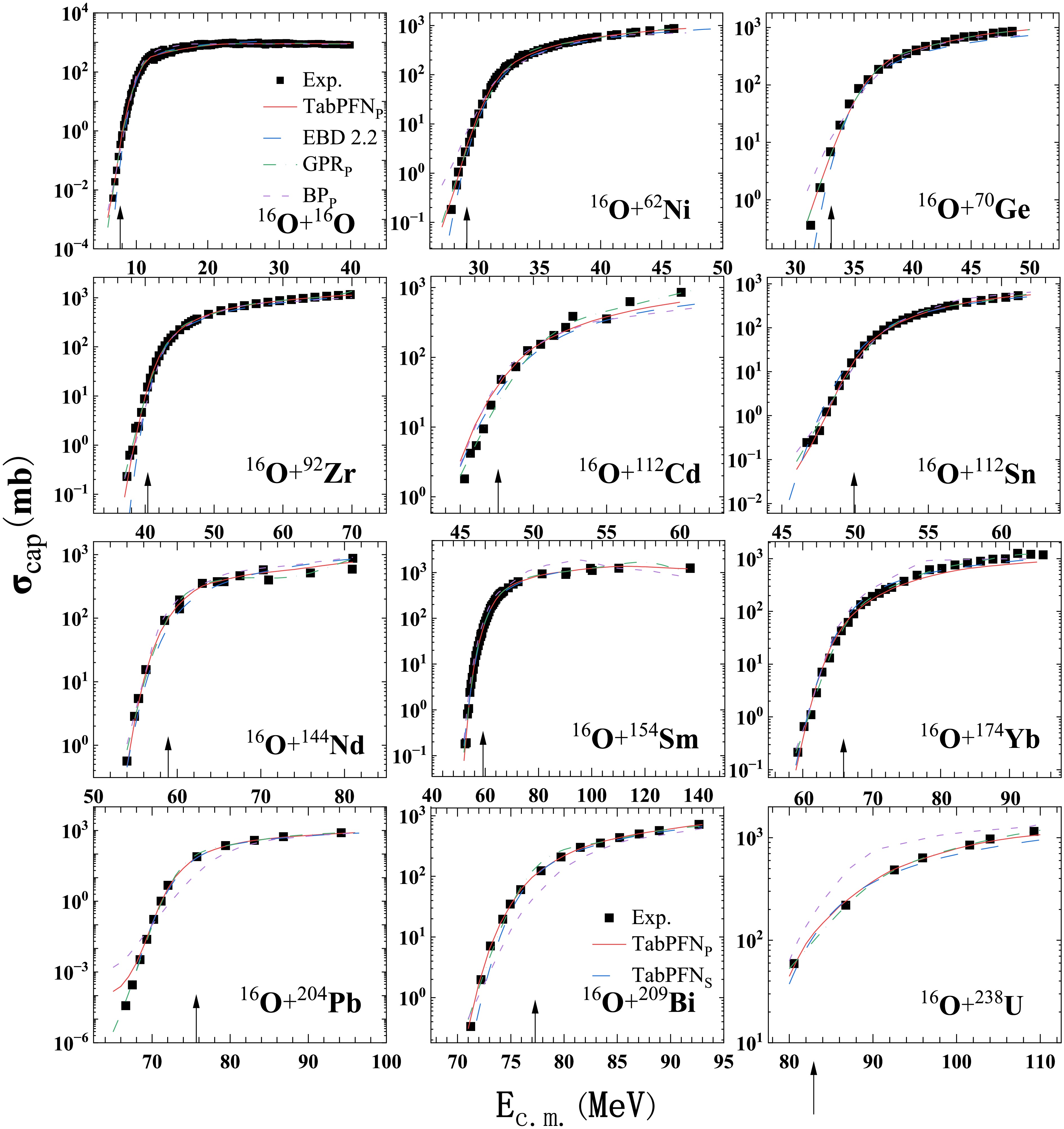

Figure 2.  (color online) Capture cross sections are compared with the available experimental data for the reactions $ ^{16} {\rm{O}}$ + $ ^{16} {\rm{O}}$ [53], $ ^{16} {\rm{O}}$ + $ ^{62} {\rm{Ni}}$ [54], $ ^{16} {\rm{O}}$ + $ ^{70} {\rm{Ge}}$ [55], $ ^{16} {\rm{O}}$ + $ ^{92} {\rm{Zr}}$ [56], $ ^{16} {\rm{O}}$ + $ ^{112} {\rm{Cd}}$ [57], $ ^{16} {\rm{O}}$ + $ ^{112} {\rm{Sn}}$ [58], $ ^{16} {\rm{O}}$ + $ ^{144} {\rm{Nd}}$ [59], $ ^{16} {\rm{O}}$ + $ ^{154} {\rm{Sm}}$ [60], $ ^{16} {\rm{O}}$ + $ ^{174} {\rm{Yb}}$ [61], $ ^{16} {\rm{O}}$ + $ ^{204} {\rm{Pb}}$ [62], $ ^{16} {\rm{O}}$ + $ ^{209} {\rm{Bi}}$ [63], and $ ^{16} {\rm{O}}$ + $ ^{238} {\rm{U}}$ [64]. The solid black squares denote the experimental data. The cross-section values predicted by different machine-learning models and an analytical formula are represented by lines: red for TabPFN_P, blue for EBD 2.2, green for GPR_P, and purple for BP_P. All machine-learning curves in this figure are generated using the point-wise random split (subscript P), in which individual energy data points are randomly assigned to the training or test sets. The proton numbers of the target nuclei range from 8 to 92, covering light to heavy nuclei. The black arrow in the figure indicates the barrier height.

While Fig. 2 evaluates model performance under point-wise interpolation, Fig. 3 further investigates model behaviour under the system-wise-split scheme (subscript S). In this scheme, the entire projectile-target combination is treated as the basic partitioning unit; each complete projectile-target pair is allocated either to the training set or to the test set. The reaction systems displayed in Fig. 3 correspond to test-set projectile-target pairs under this S-split protocol. This figure includes twelve $ ^{18}\text{O} $-induced reaction systems and displays predictions from TabPFN_S, GPR_S, BP_S, and the EBD 2.2 analytical model. Even in this more challenging system-partitioned test-set prediction scenario, TabPFN_S yields the most consistent agreement with experimental measurements among the machine-learning models. In comparison, the performance of GPR_S deteriorates substantially for many systems. As discussed in Sec. III.A, GPR employs a fixed Matérn 5/2 kernel, which cannot adequately represent strong nonlinear behaviour such as fusion hindrance and the exponential fall-off of capture cross sections in the deep-sub-barrier region. This limitation is strongly amplified when predictions are made for projectile-target pairs assigned to the test set under a system-wise split. Meanwhile, BP_S continues to show systematic deviations in several sub-barrier cases, consistent with its limited ability to model subtle channel-coupling and nuclear-structure-related suppression effects.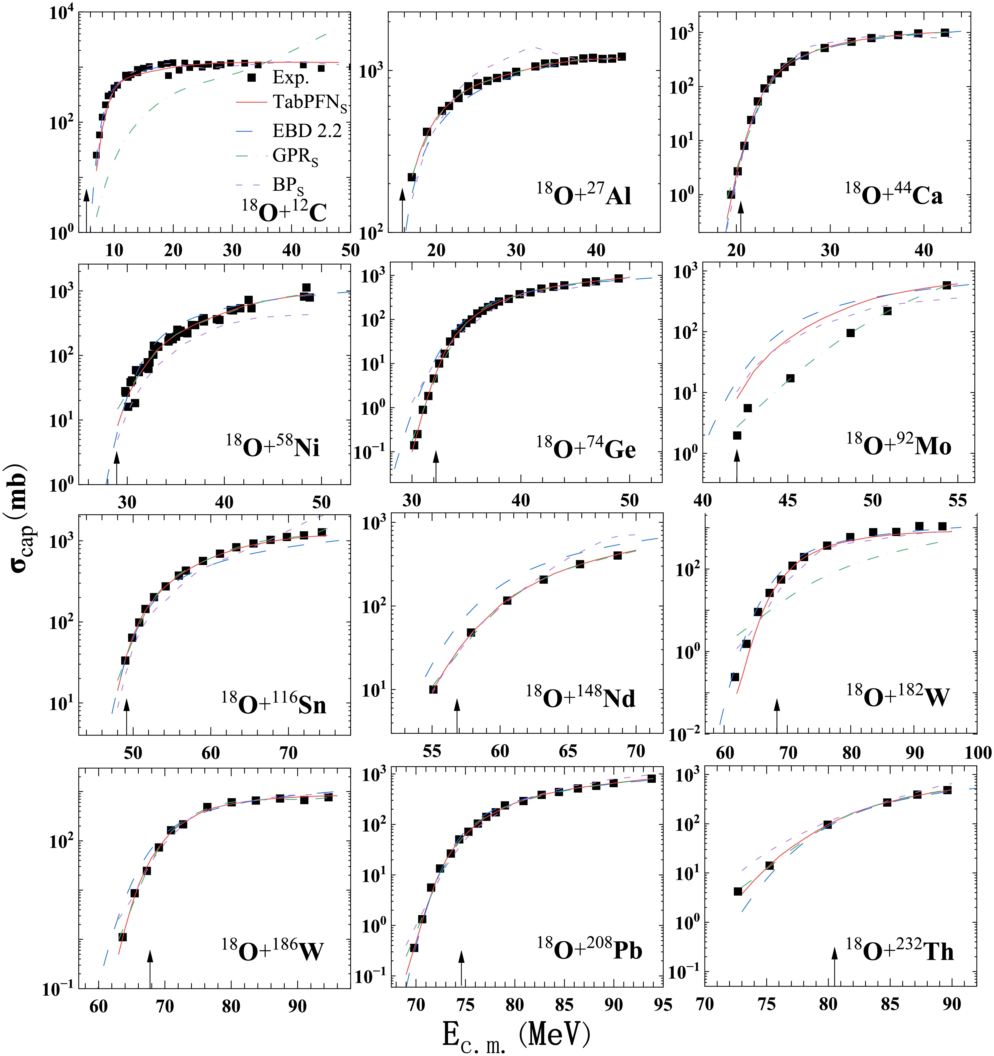

Figure 3.  (color online) Capture cross sections are compared with the available experimental data for the reactions $ ^{18} {\rm{O}}$ + $ ^{12} {\rm{C}}$ [67], $ ^{18} {\rm{O}}$ + $ ^{27} {\rm{Al}}$ [68], $ ^{18} {\rm{O}}$ + $ ^{44} {\rm{Ca}}$ [69], $ ^{18} {\rm{O}}$ + $ ^{58} {\rm{Ni}}$ [70], $ ^{18} {\rm{O}}$ + $ ^{74} {\rm{Ge}}$ [71], $ ^{18} {\rm{O}}$ + $ ^{92} {\rm{Mo}}$ [72], $ ^{18} {\rm{O}}$ + $ ^{116} {\rm{Sn}}$ [73], $ ^{18} {\rm{O}}$ + $ ^{148} {\rm{Nd}}$ [74], $ ^{18} {\rm{O}}$ + $ ^{182,186} {\rm{W}}$ [75], $ ^{18} {\rm{O}}$ + $ ^{208} {\rm{Pb}}$ [63], and $ ^{18} {\rm{O}}$ + $ ^{232} {\rm{Th}}$ [76]. Solid black squares denote the experimental data. Predicted cross sections from the different machine-learning models and the analytical formula are shown as lines: red for TabPFN_S, blue for EBD 2.2, green for GPR_S, and purple for BP_S. The predictions shown here are obtained using the system-wise split (subscript S): each complete projectile-target combination is used as the partitioning unit and is assigned entirely to either the training or the test set. The plotted systems correspond to the test-set projectile-target pairs under this splitting protocol. The black arrow indicates the barrier height.

Taken together, the comparisons in Fig. 2 (point-wise-split interpolation, P) and Fig. 3 (system-wise-split test-set prediction, S) demonstrate that TabPFN achieves the best overall performance among the three machine-learning models under both point-wise interpolation and system-partitioned test-set prediction conditions. GPR and BP show notable systematic errors in either or both scenarios, arising from their respective model-architecture limitations. For this reason, we omit GPR and BP outputs in the subsequent figures and focus exclusively on TabPFN predictions.

Given that TabPFN is selected as the primary model, Fig. 4 and Fig. 5 show side-by-side comparisons with experimental capture-cross-section values for $ ^{40}\text{Ca} $-induced and $ ^{58}\text{Ni} $-induced reactions, respectively. These projectile nuclei are either singly or doubly magic, providing useful test cases for investigating entrance-channel physical effects. Plotting both variants in the same panel enables a direct visual comparison between predictions obtained from point-wise-split interpolation (TabPFN_P, red solid lines) and system-wise-split test-set prediction (TabPFN_S, blue solid lines) for identical projectile-target combinations.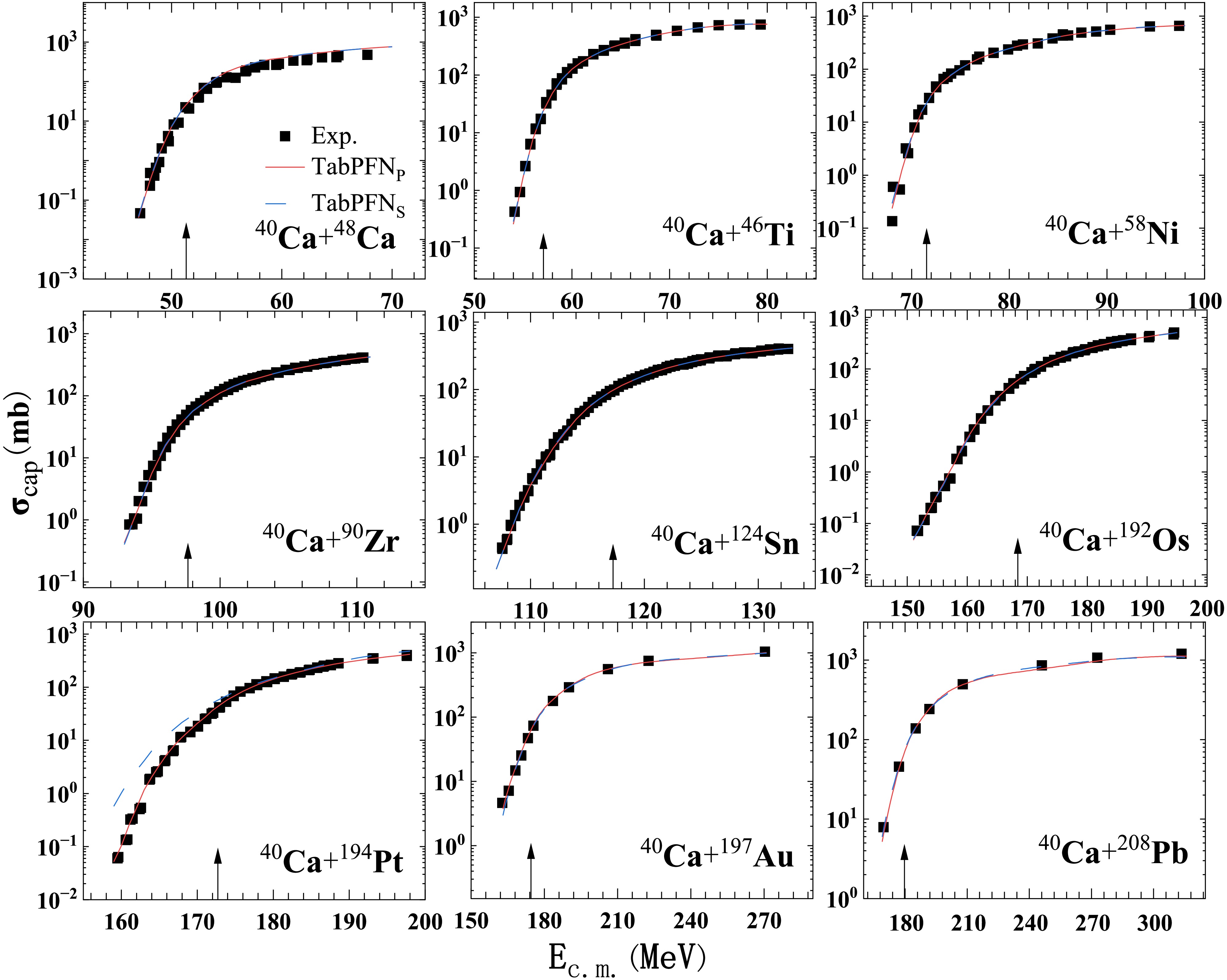

Figure 4.  (color online) Comparison of experimental capture cross-section measurements with predictions from the TabPFN model for reactions induced by $ ^{40}\text{Ca} $ projectiles. Solid black squares denote the experimental capture cross-section data, and solid red lines show predictions from TabPFN_P obtained under the pointwise random-split interpolation scheme, in which individual energy data points are randomly assigned to the training or test sets. Solid blue lines correspond to TabPFN_S results obtained under the system-wise-split protocol. In this protocol, each complete projectile-target combination is used as the partitioning unit and assigned in its entirety to either the training set or the test set. The displayed curves correspond to predictions for test-set projectile-target pairs under this splitting strategy. The plotted systems are $ ^{40} {\rm{Ca}}$ + $ ^{48} {\rm{Ca}}$ [77], $ ^{40} {\rm{Ca}}$ + $ ^{46} {\rm{Ti}}$ [78], $ ^{40} {\rm{Ca}}$ + $ ^{58} {\rm{Ni}}$ [79], $ ^{40} {\rm{Ca}}$ + $ ^{90} {\rm{Zr}}$ [80], $ ^{40} {\rm{Ca}}$ + $ ^{124} {\rm{Sn}}$ [81], $ ^{40} {\rm{Ca}}$ + $ ^{192} {\rm{Os}}$ [82], $ ^{40} {\rm{Ca}}$ + $ ^{194} {\rm{Pt}}$ [82], $ ^{40} {\rm{Ca}}$ + $ ^{197} {\rm{Au}}$ [83], and $ ^{40} {\rm{Ca}}$ + $ ^{208} {\rm{Pb}}$ [83]. The proton numbers of the target nuclei range from 20 to 82, spanning light to heavy nuclei. The black arrow in the figure indicates the barrier height.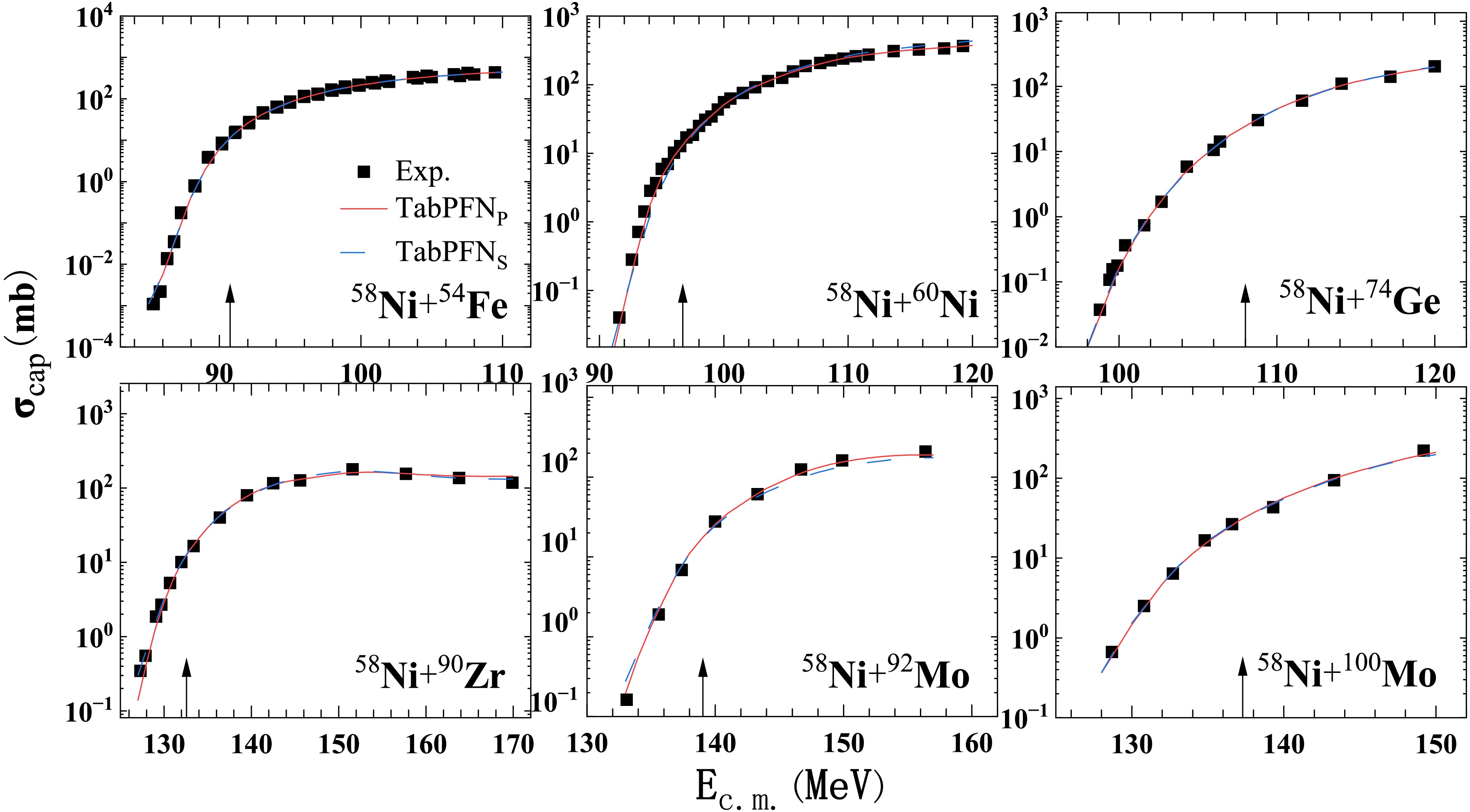

Figure 5.  (color online) The same as in Fig. 4, but for the reactions $ ^{58} {\rm{Ni}}$ + $ ^{54} {\rm{Fe}}$ [84], $ ^{58} {\rm{Ni}}$ + $ ^{60} {\rm{Ni}}$ [85], $ ^{58} {\rm{Ni}}$ + $ ^{74} {\rm{Ge}}$ [86], $ ^{58} {\rm{Ni}}$ + $ ^{90} {\rm{Zr}}$ [87], and $ ^{58} {\rm{Ni}}$ + $ ^{92,100} {\rm{Mo}}$ [88]. The black arrow indicates the barrier height.

Extensive experimental and theoretical studies have established that heavy-ion fusion dynamics are governed by the coupling of the relative motion of colliding nuclei [89] to intrinsic nuclear degrees of freedom. Widely used theoretical frameworks, including the modified EBD model [18], empirical coupled-channel (ECC) model [21, 22], and Wong formula [23, 51], generally reproduce near-barrier experimental capture cross sections well, but may produce non-negligible overpredictions or underpredictions for certain systems in the sub-barrier domain. As shown in Fig. 4 and Fig. 5, TabPFN can satisfactorily reproduce experimental capture-cross-section values even at sub-barrier energies. We further utilise these datasets to examine whether TabPFN can recover well-known entrance-channel-driven physical trends, particularly the influences of mass asymmetry and charge asymmetry on sub-barrier capture cross sections.

The mass asymmetry, $ \eta_A $, and charge asymmetry, $ \eta_Z $, are defined as

where $ A_{1} $ and $ A_{2} $, and $ Z_{1} $ and $ Z_{2} $, are the mass and atomic numbers of the projectile and target nuclei, respectively. Figure 6 presents the TabPFN_S predictions and experimental values of the capture cross sections for two combinations forming the same compound nucleus, $ ^{128}{\rm{Ba}} $ ($ ^{32} {\rm{S}}$ + $ ^{96} {\rm{Zr}}$ and $ ^{64} {\rm{Ni}}$ + $ ^{64} {\rm{Ni}}$), and two combinations forming the same compound nucleus, $ ^{136} {\rm{Sm}}$ ($ ^{32} {\rm{S}}$ + $ ^{104} {\rm{Pd}}$ and $ ^{46} {\rm{Ti}}$ + $ ^{90} {\rm{Zr}}$). To distinguish above-barrier from below-barrier energies, the horizontal axis represents the center-of-mass energy relative to the barrier height; thus, 0 corresponds to the Bass barrier. Previous studies have shown that, for different projectile–target combinations forming the same compound nucleus, systems with larger mass asymmetry may exhibit larger cross sections at sub-barrier energies because of enhanced coupling effects [94]. In the present cases, the combinations with greater mass asymmetry, namely $ ^{32} {\rm{S}}$ + $ ^{96} {\rm{Zr}}$ ($ \eta_A = 0.5 $) and $ ^{32} {\rm{S}}$ + $ ^{104} {\rm{Pd}}$ ($ \eta_A = 0.53 $), also have larger charge asymmetry ($ \eta_Z = 0.43 $ and $ \eta_Z = 0.48 $, respectively) than their less asymmetric counterparts ($ ^{64} {\rm{Ni}}$ + $ ^{64} {\rm{Ni}}$: $ \eta_A = 0 $, $ \eta_Z = 0 $; $ ^{46} {\rm{Ti}}$ + $ ^{90} {\rm{Zr}}$: $ \eta_A = 0.32 $, $ \eta_Z = 0.29 $). The combined effects of mass and charge asymmetry lead to stronger coupling to inelastic excitations and transfer channels, thereby enhancing the sub-barrier fusion probability. Consequently, these systems exhibit larger capture cross sections at below-barrier energies, indicating a higher tunneling probability through the Coulomb barrier. The employed machine learning method therefore yields results consistent with the expected joint influence of mass and charge asymmetry on the capture process.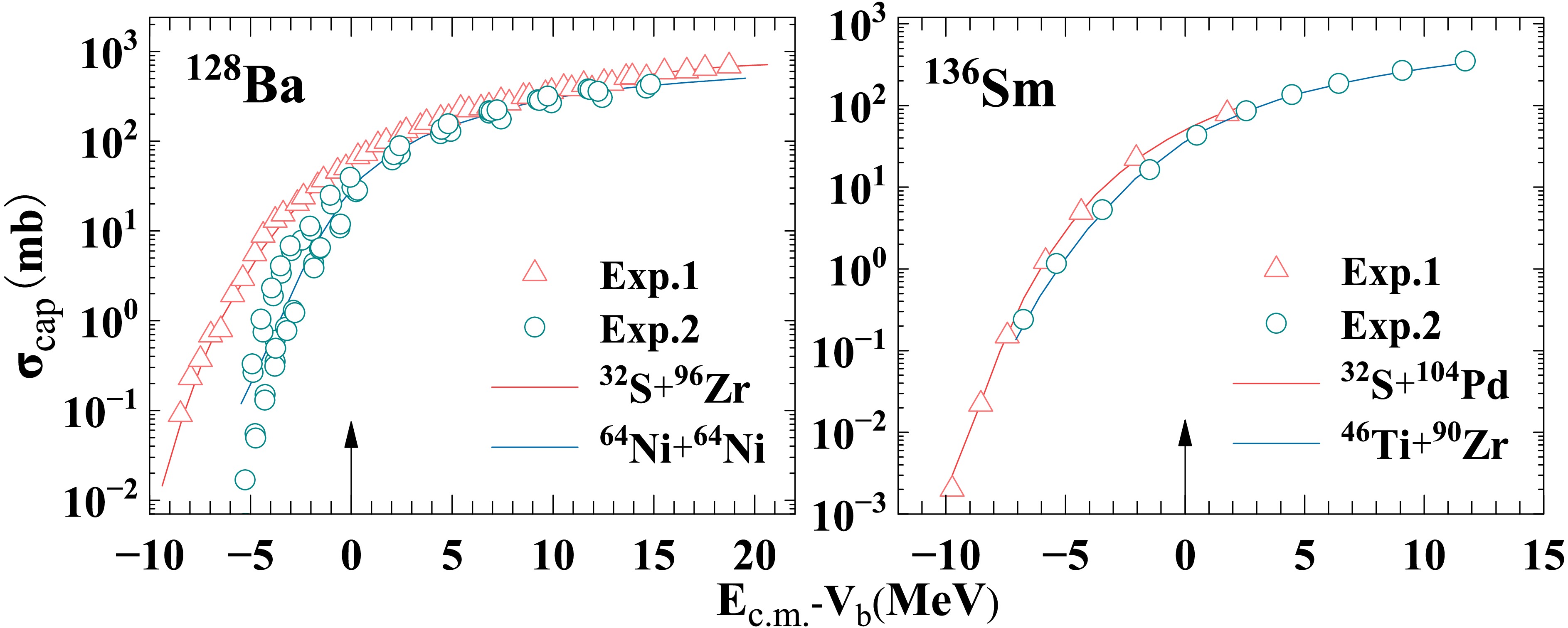

Figure 6.  (color online) The figure compares the TabPFN_S-predicted theoretical capture cross sections with the corresponding experimental values for two sets of entrance-channel systems leading to the same compound nucleus. The left panel shows systems forming the compound nucleus $ ^{128} {\rm{Ba}}$. Red open triangles and solid red lines represent the experimental cross sections and the TabPFN_S-predicted theoretical values for $ ^{32} {\rm{S}}$ + $ ^{96} {\rm{Zr}}$ [90], respectively, whereas blue open circles and solid blue lines represent those for $ ^{64} {\rm{Ni}}$ + $ ^{64} {\rm{Ni}}$ [91]. The right panel shows systems forming the compound nucleus $ ^{136} {\rm{Sm}}$. Red open triangles and solid red lines denote $ ^{32} {\rm{S}}$ + $ ^{104} {\rm{Pd}}$ [92], whereas blue open circles and solid blue lines denote $ ^{46} {\rm{Ti}}$ + $ ^{90} {\rm{Zr}}$ [93]. Notably, the systems $ ^{32} {\rm{S}}$ + $ ^{96} {\rm{Zr}}$ and $ ^{32} {\rm{S}}$ + $ ^{104} {\rm{Pd}}$ exhibit greater mass and charge asymmetries. The black arrow in the figure indicates the barrier height.

To investigate another key entrance-channel factor, we examine the influence of neutron asymmetry. The formula for neutron asymmetry is given by

where $ N_{1} $ and $ N_{2} $ are the neutron numbers of the projectile and target nuclei, respectively. Figure 7 presents the TabPFN_S predictions together with the theoretical and experimental capture cross-section values for two pairs of projectile–target combinations that form the same compound nuclei: $ ^{124} {\rm{Sn}}$ + $ ^{48} {\rm{Ca}}$ and $ ^{132} {\rm{Sn}}$ + $ ^{40} {\rm{Ca}}$ both lead to $ ^{172} {\rm{Yb}}$, whereas $ ^{16} {\rm{O}}$ + $ ^{76} {\rm{Ge}}$ and $ ^{18} {\rm{O}}$ + $ ^{74} {\rm{Ge}}$ both lead to $ ^{92} {\rm{Zr}}$. In the sub-barrier region, the capture cross-section curves for the two combinations forming $ ^{92} {\rm{Zr}}$ essentially overlap despite their different neutron asymmetries. Notably, the difference in μ values between these two systems is relatively small, which may partly account for the negligible influence of neutron asymmetry in this case. For the two combinations forming $ ^{172} {\rm{Yb}}$, the system with the higher neutron asymmetry μ, $ ^{132} {\rm{Sn}}$ + $ ^{40} {\rm{Ca}}$, exhibits a significantly larger capture cross section. These observations suggest that the effect of neutron asymmetry on sub-barrier fusion may be system-dependent. Although a larger difference in μ appears to correlate with enhanced fusion in the $ ^{172} {\rm{Yb}}$ case, the overlapping curves for the $ ^{92} {\rm{Zr}}$ case indicate that this effect is not universal. Because only one pair shows a clear difference, we refrain from drawing a definitive conclusion and emphasize that further systematic studies with more projectile–target combinations are needed to clarify the role of neutron asymmetry.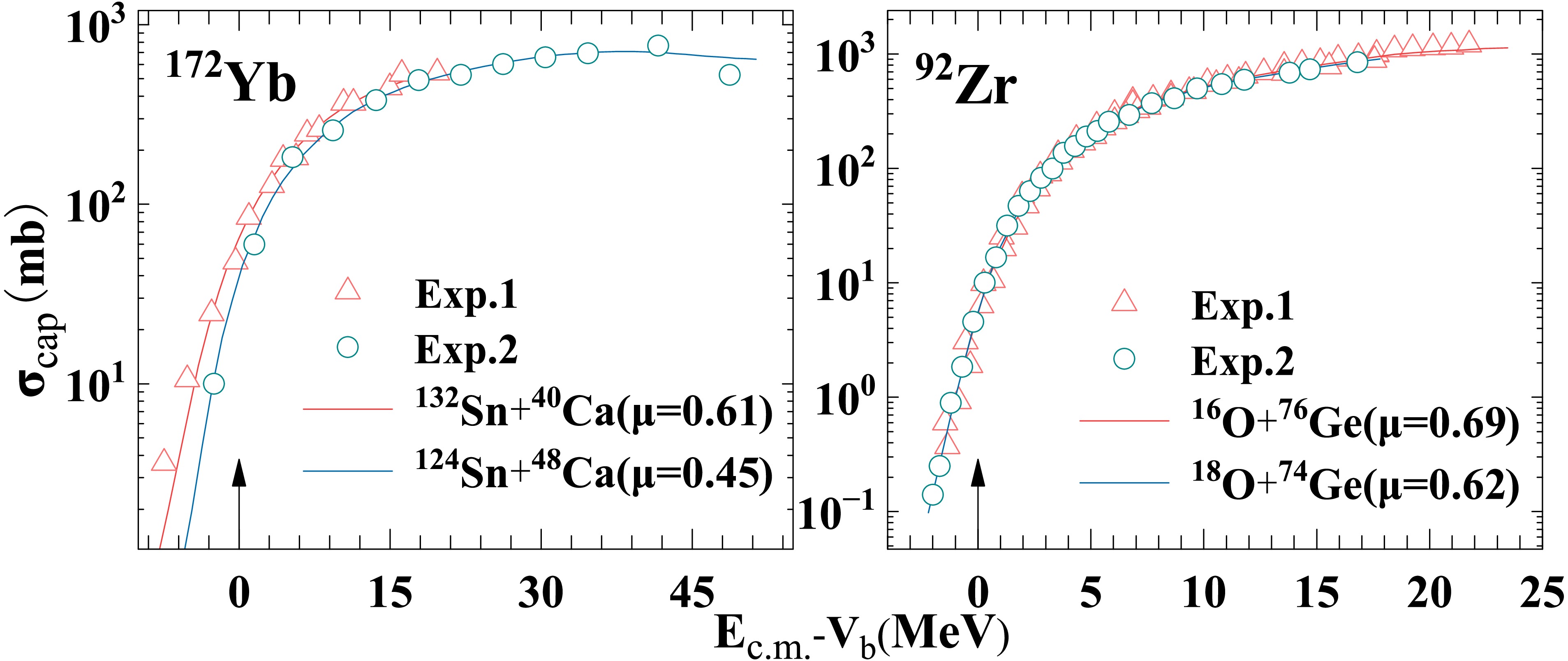

Figure 7.  (color online) The figure compares the TabPFN_S-predicted theoretical capture cross sections with the corresponding experimental values for two sets of entrance-channel systems leading to the same compound nucleus. The left panel shows systems forming the compound nucleus $ ^{172} {\rm{Yb}}$. The red hollow triangles and solid red lines represent the experimental cross sections and the TabPFN_S-predicted theoretical values, respectively, for $ ^{132} {\rm{Sn}}$ + $ ^{40} {\rm{Ca}}$ [95], whereas the blue hollow circles and solid blue lines represent the corresponding results for $ ^{124} {\rm{Sn}}$ + $ ^{48} {\rm{Ca}}$ [95]. The right panel shows systems forming the compound nucleus $ ^{92} {\rm{Zr}}$. Using the same convention, the red hollow triangles and solid red lines denote $ ^{16} {\rm{O}}$ + $ ^{76} {\rm{Ge}}$ [55], and the blue hollow circles and solid blue lines denote $ ^{18} {\rm{O}}$ + $ ^{74} {\rm{Ge}}$ [55]. The neutron asymmetry values for each reaction are indicated in parentheses. The black arrow in the figure marks the barrier height.

Based on the preceding analysis of how entrance-channel effects, such as mass asymmetry η and neutron asymmetry μ, influence the capture cross section, we further extend the discussion to the extrapolation of cross-section data. In nuclear reaction research, experimental measurements are often confined to specific energy regions and nuclear combinations. However, in many important contexts—such as the synthesis of key nuclides in astrophysical environments, the estimation of cross sections for producing superheavy elements, and the exploration of nuclear-structure effects under extreme conditions—reliable extrapolation of cross sections into unmeasured regions is essential. The accuracy of such extrapolation directly affects the credibility of theoretical predictions. Therefore, developing predictive methods with robust extrapolation capabilities is crucial for expanding the applicability of nuclear reaction data and reducing prediction uncertainties.

The point-wise random splitting strategy adopted above distributes energy points belonging to the same reaction system across the training and test sets. Although this scheme can characterize interpolation accuracy, it does not quantitatively evaluate the genuine extrapolation performance of the model for fully unknown projectile-target pairs. To address this limitation and rigorously examine the in-distribution generalization capacity of the model, we perform leave-one-system-out cross-validation (LOSO-CV). Using an identical LOSO-CV protocol, ablation experiments are carried out to compare the baseline 5-feature TabPFN model—that is, using only the proton numbers and mass numbers of the projectile and target nuclei ($ Z_P $, $ Z_T $, $ A_P $, $ A_T $) and the center-of-mass energy ($ E_\mathrm{c.m.} $) as inputs—with the full-input 13-feature TabPFN model that incorporates entrance-channel-related physical quantities. In this validation scheme, one complete projectile-target combination is excluded as the test set in each iteration, and all remaining systems are used for training. The group-wise mean absolute error (MAE) for each projectile-target system is calculated following Eq. (3) and is defined as the arithmetic average of the absolute errors over all data points within a single reaction system, yielding independent extrapolation-error measurements for every investigated reaction system.

We further clarify the data-processing pipeline within each fold of the leave-one-system-out cross-validation (LOSO-CV).

(1) Missing-feature handling: After dataset cleaning, the 13 selected input features contain no missing values for all retained samples. Raw entries with any missing derived physical quantities were completely excluded in the preprocessing stage before model training; therefore, no imputation step is required in the model pipeline.

(2) Fold-level independent normalization: Within each LOSO-CV fold, the mean and standard deviation for z-score standardization are calculated only from the training subset of that specific fold. The held-out test samples are transformed using these training-set-derived statistics. Global dataset-wide normalization is never performed before cross-validation, strictly avoiding test-set information leakage.

(3) No additional filtering within folds: No additional sample-level or feature-level filtering is executed within individual LOSO-CV validation folds. All filtering operations are completed during the dataset-cleaning phase before any cross-validation run.

The statistical distributions of the group-wise MAE for the 5-feature and 13-feature models are displayed in Fig. 8 and Fig. 9, respectively. As illustrated in Fig. 8 for the 5-feature baseline model, the median MAE over all 566 systems is 0.108, with an overall mean MAE of 0.159 and a maximum of 1.857. For the 13-feature full-input model shown in Fig. 9, the median MAE across all 566 systems is 0.107, with an overall mean MAE of 0.157 and a maximum of 2.066. For both models, the mean value is considerably higher than the median, indicating a distinctly right-skewed error distribution. A small subset of systems exhibits relatively large group-wise MAE values. These challenging reaction systems are further analysed in Table A1 in Appendix A, and the corresponding excitation-function comparison plots for the most difficult cases ($ \overline{{\mathrm{MAE}}}>1 $) are provided in Fig. A1 in Appendix A. After excluding the most challenging high-MAE systems, the main distributions in Fig. 8(b) and Fig. 9(b) show that extrapolation errors for the vast majority of systems are concentrated within the low-error interval of 0−0.25; only a small fraction of systems show notable prediction deviations. According to the interval statistics from Fig. 8(c) and Fig. 9(c), 46.8% of reaction systems achieve $ {{\mathrm{MAE}}}<0.1 $ for the 5-feature model, compared with 46.6% for the 13-feature model. In total, 95.6% of systems (541) for the 5-feature model and 96.1% of systems (544) for the 13-feature model satisfy $ {{\mathrm{MAE}}}\le 0.5 $. In addition, only 3 systems (0.5%) in the 13-feature model exhibit $ {{\mathrm{MAE}}}>1 $.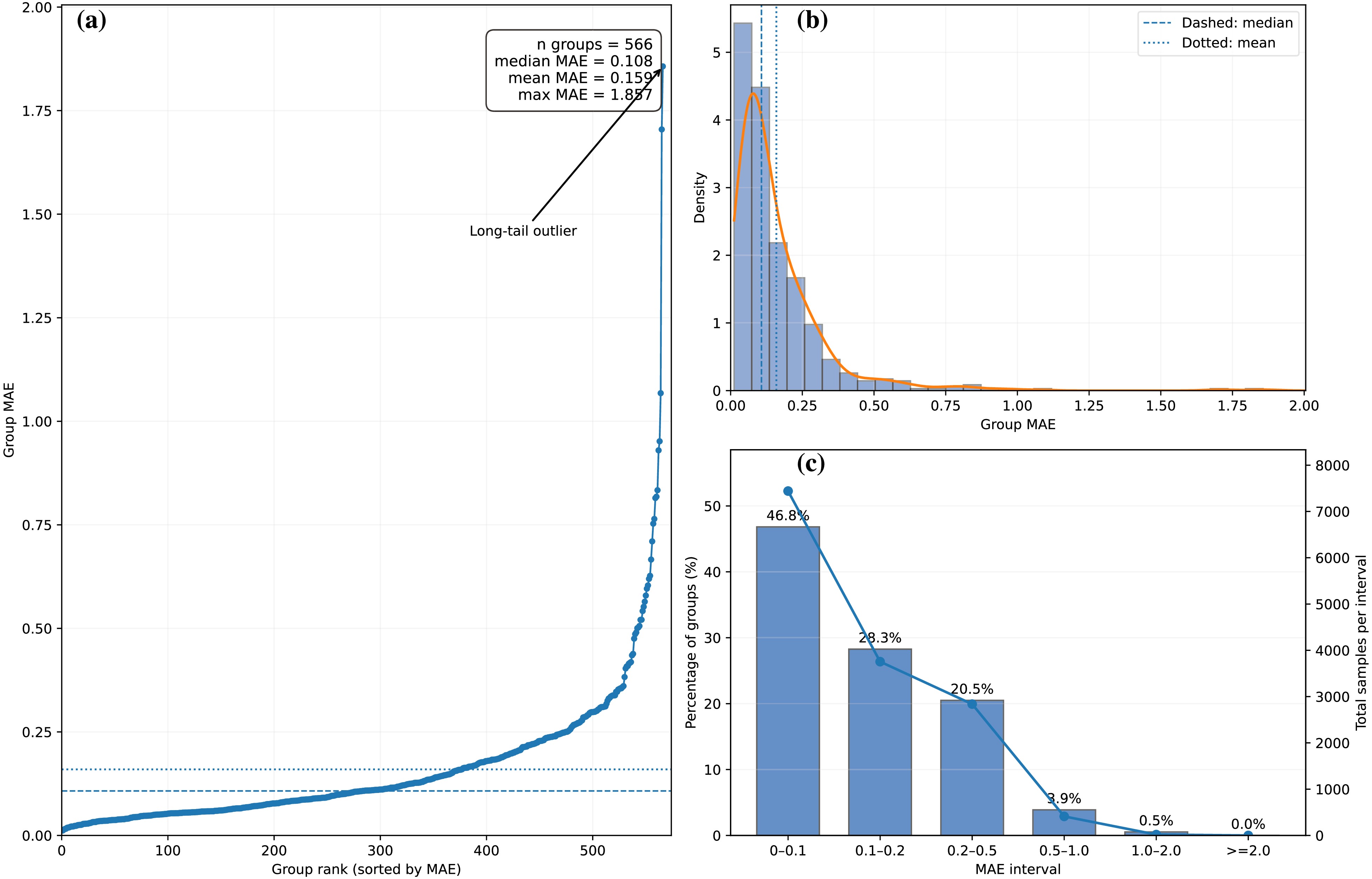

Figure 8.  (color online) Group-wise MAE distribution from leave-one-system-out cross-validation for the 5-feature TabPFN model across 566 projectile-target systems. (a) Sorted MAE values for all systems, with inset statistics: median 0.108, mean 0.159, and maximum 1.857. A small subset of systems exhibits comparatively large group-wise MAE values, corresponding to challenging reaction systems. (b) Histogram and kernel-density estimate of the group-wise MAE within the 99% data range after excluding the most challenging high-MAE systems. The blue dashed line denotes the median MAE, and the blue dotted line denotes the mean MAE; the distribution exhibits pronounced right skewness. (c) Bar chart showing the fraction of reaction systems within each MAE interval (left vertical axis), with the solid blue curve denoting the total number of data samples within each interval (right vertical axis). A total of 95.6% of systems achieve $ {\mathrm{MAE}} \le 0.5 $.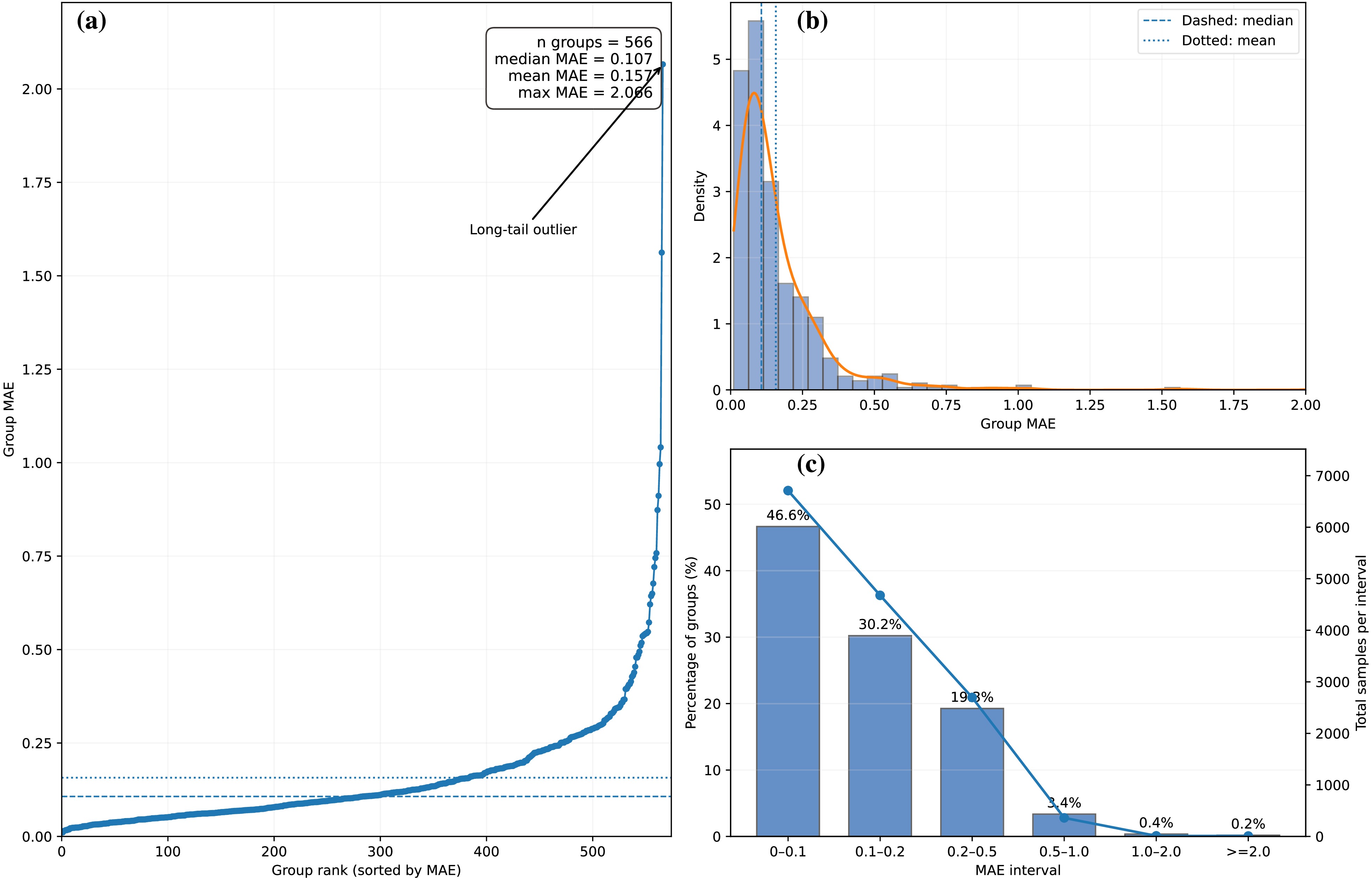

Figure 9.  (color online) Group-wise MAE distribution obtained from leave-one-system-out cross-validation for the full 13-feature TabPFN model across 566 projectile–target systems. (a) Sorted MAE values for all systems, with inset statistics showing a median of 0.107, a mean of 0.157, and a maximum of 2.066. (b) Histogram and kernel-density estimate of group-wise MAE within the 99% data range after excluding extreme outliers. The blue dashed line denotes the median MAE, and the blue dotted line denotes the mean MAE; the distribution is right-skewed. (c) Bar chart showing the fraction of reaction systems within each MAE interval (left vertical axis), while the solid blue curve represents the total number of data samples within each interval (right vertical axis). Overall, 96.1% of systems achieve $ {\mathrm{MAE }}\le 0.5 $.

It is noteworthy that most high-MAE systems listed in Table A1 in Appendix A are constrained by relatively sparse experimental measurements. These 22 systems have a median of 11.5 experimental data points, and 10 of them contain no more than 10 measured points. Several of these challenging systems also exhibit pronounced entrance-channel mass asymmetry. Figure A1 in Appendix A provides excitation-function comparisons between experimental observations and model predictions for systems with $ {\mathrm{MAE}}>0.75 $, allowing detailed inspection of these difficult cases.

The ablation comparison demonstrates that adding eight supplementary entrance-channel-related physical features does not yield a prominent reduction in the global overall MAE relative to the 5-feature baseline. Nevertheless, the 13-feature model explicitly encodes entrance-channel-relevant physical observables as model inputs. As presented in Sec. III.B, the 13-feature TabPFN is capable of reproducing well-known physical trends induced by mass and charge asymmetry in sub-barrier capture reactions.

To further quantitatively investigate how prediction performance varies with collision energy under in-distribution generalization conditions, we analyse residuals obtained from LOSO-CV predictions of the 13-feature TabPFN across all 566 projectile-target combinations, as shown in Fig. 10. The dataset is divided into five bins according to the relative energy $ E_\mathrm{c.m.}-V_b $, where $ V_b $ denotes the Bass Coulomb barrier height, and the binning scheme is summarised in Table 2. Each bin is characterised by the median value of $ E_\mathrm{c.m.}-V_b $ for the contained samples.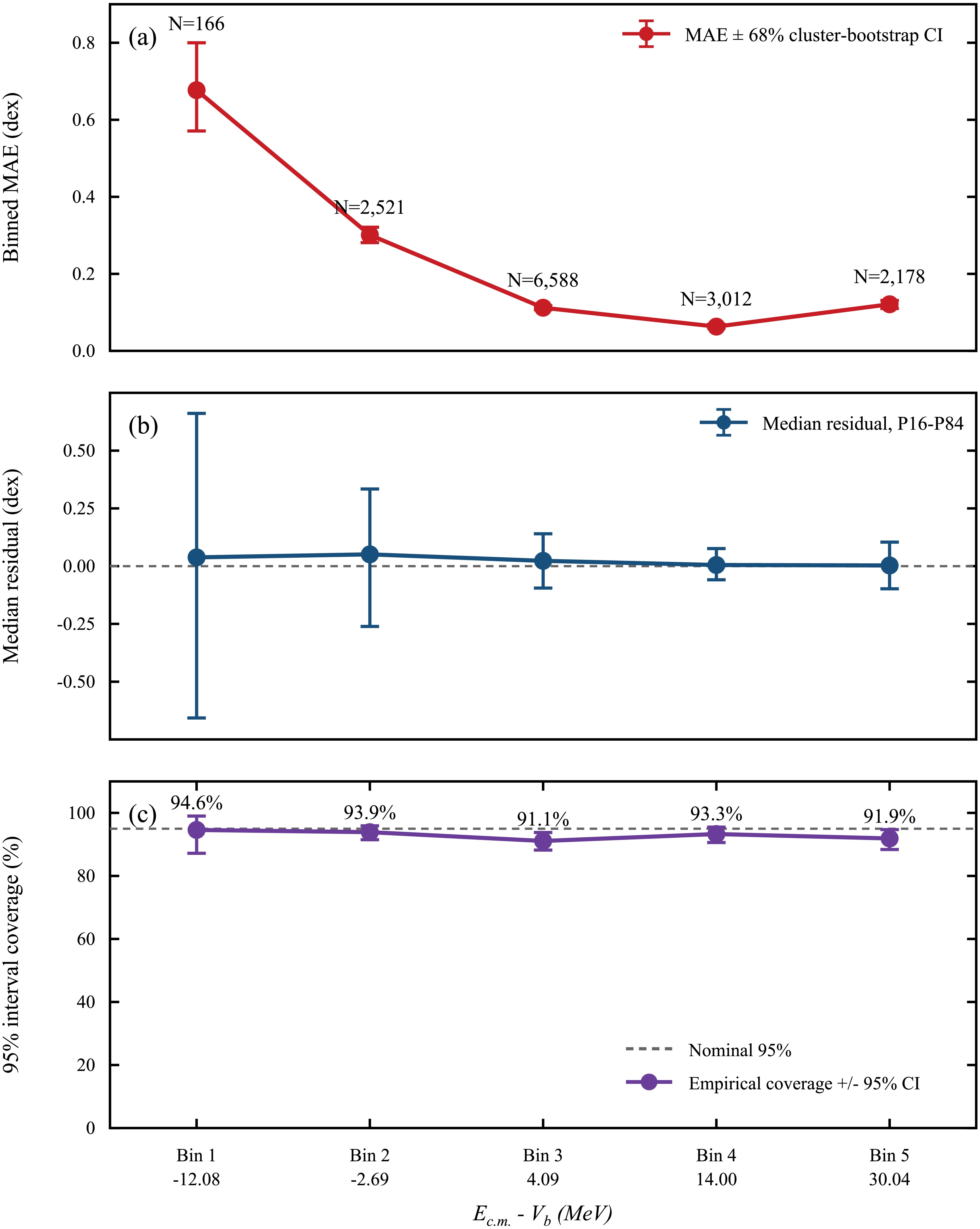

Figure 10.  (color online) Energy-binned statistical analysis of the LOSO-CV predictions of the 13-feature TabPFN model for 566 projectile–target systems, comprising 14 465 experimental data points. The bins are defined by $ E_{\mathrm{c.m.}}-V_b $, as specified in Table 2, and each bin is plotted at the median value of $ E_{\mathrm{c.m.}}-V_b $. (a) Binned mean absolute error (MAE; in dex). Error bars denote the 68% cluster-bootstrap confidence intervals obtained by resampling at the projectile–target-system level; the number of data points in each bin is annotated. (b) Median signed residual, $ r=\log_{10}\sigma_{\mathrm{exp}}-\log_{10}\sigma_{\mathrm{pred}} $. Error bars indicate the P16–P84 percentile range, and the horizontal dashed line marks zero residual. (c) Empirical coverage of the nominal 95% prediction intervals in each energy bin. Error bars denote the 95% confidence intervals for the estimated coverage, and the horizontal dashed line indicates the nominal 95% coverage level.

Figure 10(a) presents the binned mean absolute error (MAE, unit: dex) for each energy bin, with error bars representing the 68% cluster-bootstrap confidence interval. These confidence intervals are estimated by drawing 10 000 bootstrap resamples with replacement at the full projectile-target-system level to account for intra-system correlation. The number of data points in each bin is annotated. Figure 10(b) shows the median signed residuals $ r=\log_{10}\sigma_\mathrm{exp}-\log_{10}\sigma_\mathrm{pred} $, together with the P16–P84 percentile range describing residual dispersion. Figure 10(c) shows the empirical coverage corresponding to TabPFN's native 2.5%−97.5% quantile prediction intervals. The coverage values for bins 1−5 are 94.6%, 93.9%, 91.1%, 93.3%, and 91.9%, respectively. The prediction intervals therefore exhibit slight undercoverage in most energy regions. This result is consistent with the fact that the reported intervals are native model-generated quantile intervals without post-hoc empirical calibration.

After data correction and canonicalization, the binned statistics show that the deep-sub-barrier bin ($ E_{\mathrm{c.m.}}-V_b \lt -10\ \mathrm{MeV} $) has the largest binned mean absolute error. Because this bin contains only 166 data points and corresponds to a highly heterogeneous subset of reaction systems, this result should be interpreted as reduced prediction accuracy for the present audited dataset rather than as a universal inherent defect of the model. The median signed residuals for all five bins remain close to zero, indicating no global systematic over- or under-prediction. The full-dataset binned analysis quantitatively corroborates the energy-dependent difficulty of heavy-ion capture-cross-section prediction.

Figure 11 compares experimental capture-cross-section measurements with predictions obtained from the fully trained 13-feature TabPFN_S model for three reaction systems: $ ^{16}\text{O}+^{208}\text{Pb} $, $ ^{16}\text{O}+^{244}\text{Pu} $, and $ ^{18}\text{O}+^{184}\text{W} $. These predictions are generated from a single 8:2 system-wise split partition. The three projectile-target combinations are fully external samples excluded from both the training set and the test set of this specific partition, and they are independent of the LOSO-CV calculations presented above. They constitute local, independent, in-distribution external test cases for unseen projectile-target pairs.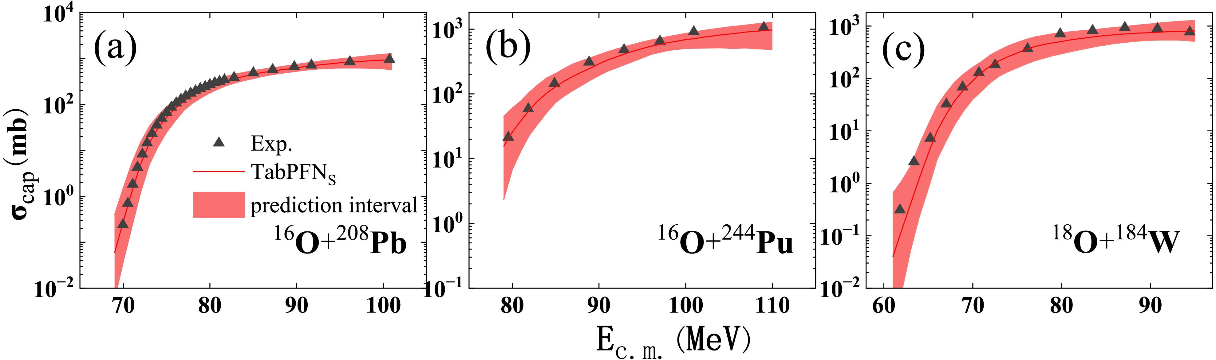

Figure 11.  (color online) A comparison is presented between theoretical predictions and experimental capture cross sections for the three reaction systems: $ ^{16} {\rm{O}}$ + $ ^{208} {\rm{Pb}}$ [96], $ ^{16} {\rm{O}}$ + $ ^{244} {\rm{Pu}}$ [97], and $ ^{18} {\rm{O}}$ + $ ^{184} {\rm{W}}$ [75]. Gray triangles represent experimental data, and the red solid line shows the mean prediction obtained from TabPFN_S. The orange shaded region corresponds to the nominal $ 95 $% prediction interval produced by TabPFN. These intervals are nominal model-generated intervals without empirical coverage calibration. These three systems serve as local, independent, in-distribution external test cases for unseen projectile-target pairs.

The red solid lines denote the mean point predictions, while the orange shaded bands correspond to the 95% prediction intervals produced by TabPFN_S. As illustrated in Fig. 11 (a) and Fig. 11 (c), the model's prediction intervals reproduce the overall trend of the experimental data (gray triangular symbols) reasonably well. Even in energy domains where training-sample coverage is sparse, the shaded prediction bands remain within physically plausible magnitude ranges. Figure 11(b) displays the predictive performance for the heavy system $ ^{16}\text{O}+^{244}\text{Pu} $. Here, the model generalizes physical patterns learned from related projectile-target pairs in the training dataset to a heavier compound-nucleus system. Even for this challenging case, the 95% prediction interval of TabPFN_S shows satisfactory consistency with the available experimental capture-cross-section data.

These results indicate that TabPFN_S not only has good fitting capabilities on known systems but also exhibits reasonable robustness for in-distribution generalization. This capability offers a useful computational tool for estimating unknown capture cross sections for reaction pairs within experimentally covered domains, especially for systems in superheavy nucleus synthesis that are challenging to measure experimentally. Future research could further explore the correspondence between model prediction uncertainty and physical mechanisms, thereby promoting deeper integration between data-driven methods and theoretical models.

This work systematically assesses three machine-learning models (TabPFN, GPR, and BP) for predicting heavy-ion capture cross sections using a dataset comprising 566 projectile-target combinations and 14 465 experimental data points. Logarithmically transformed capture-cross-section values are used, and the mean absolute error ($ \mathrm{MAE} $) serves as the evaluation metric. Two distinct data-partitioning schemes are employed: the point-wise random split (P) for interpolation assessment and the projectile-target-level system-wise split (S) for evaluating system-level predictive capability. Under point-wise-split interpolation, TabPFN_P achieves the lowest test-set $ \mathrm{MAE} $. Under the more demanding system-wise-split condition, all models exhibit substantially increased test errors; however, TabPFN_S still achieves the lowest test $ \mathrm{MAE} $. Repeated training with 100 random seeds further confirms that the performance of TabPFN_S is not dominated by a favorable single data partition.

Comparisons of capture cross sections for representative projectile-target systems demonstrate that the 13-feature model can partially reproduce the physical trends of sub-barrier capture cross sections induced by mass and charge asymmetry. The neutron-asymmetry effect exhibits evident system dependence, which requires further validation with larger datasets. Leave-one-system-out cross-validation (LOSO-CV) is performed for TabPFN_S to assess the model's in-distribution predictive behavior for fully unseen projectile-target pairs. Ablation experiments comparing the 5-feature baseline model with the full 13-feature model are conducted to investigate the influence of incorporating entrance-channel-related physical features on model outputs. The statistics show that 96.1% of unseen projectile-target pairs satisfy $ {{\mathrm{MAE}}}\le 0.5 $, and the overall distribution of group-wise $ {{\mathrm{MAE}}} $ is obtained. We also perform binned-residual statistics to extract residual information across different relative-energy bins. Three fully external reaction systems, completely excluded from the training and test datasets, are used as independent local in-distribution test cases for unseen projectile-target pairs. TabPFN_S provides reasonable pointwise mean predictions together with physically consistent 95% prediction intervals.

Collectively, our results demonstrate that TabPFN_S exhibits promising potential for in-distribution-generalization-oriented prediction of heavy-ion capture cross sections for unseen projectile-target pairs. Within the scope of the available experimental data, it achieves both quantitative prediction accuracy and partial physical consistency. Further investigations are required to disentangle the correspondence between model-output prediction uncertainty and the underlying microscopic physical mechanisms of nuclear reactions. Expanding datasets and combining machine-learning approaches with conventional nuclear-reaction theoretical models will help improve prediction reliability for unexplored domains of the nuclear-reaction landscape in future studies.

This appendix provides supplementary information for the LOSO-CV analysis presented in Sec. III.C. Table A1 summarizes the 22 projectile-target combinations with a group-wise MAE greater than 0.5 dex. For each system, we list the number of experimental data points, the group-wise MAE, the mean signed residual (Bias), and the entrance-channel mass asymmetry $ \eta_A $. Excitation-function comparison plots for the seven projectile-target combinations with group-wise $ \overline{{\mathrm{MAE}}}>0.75 $ are shown in Fig. A1 of this appendix.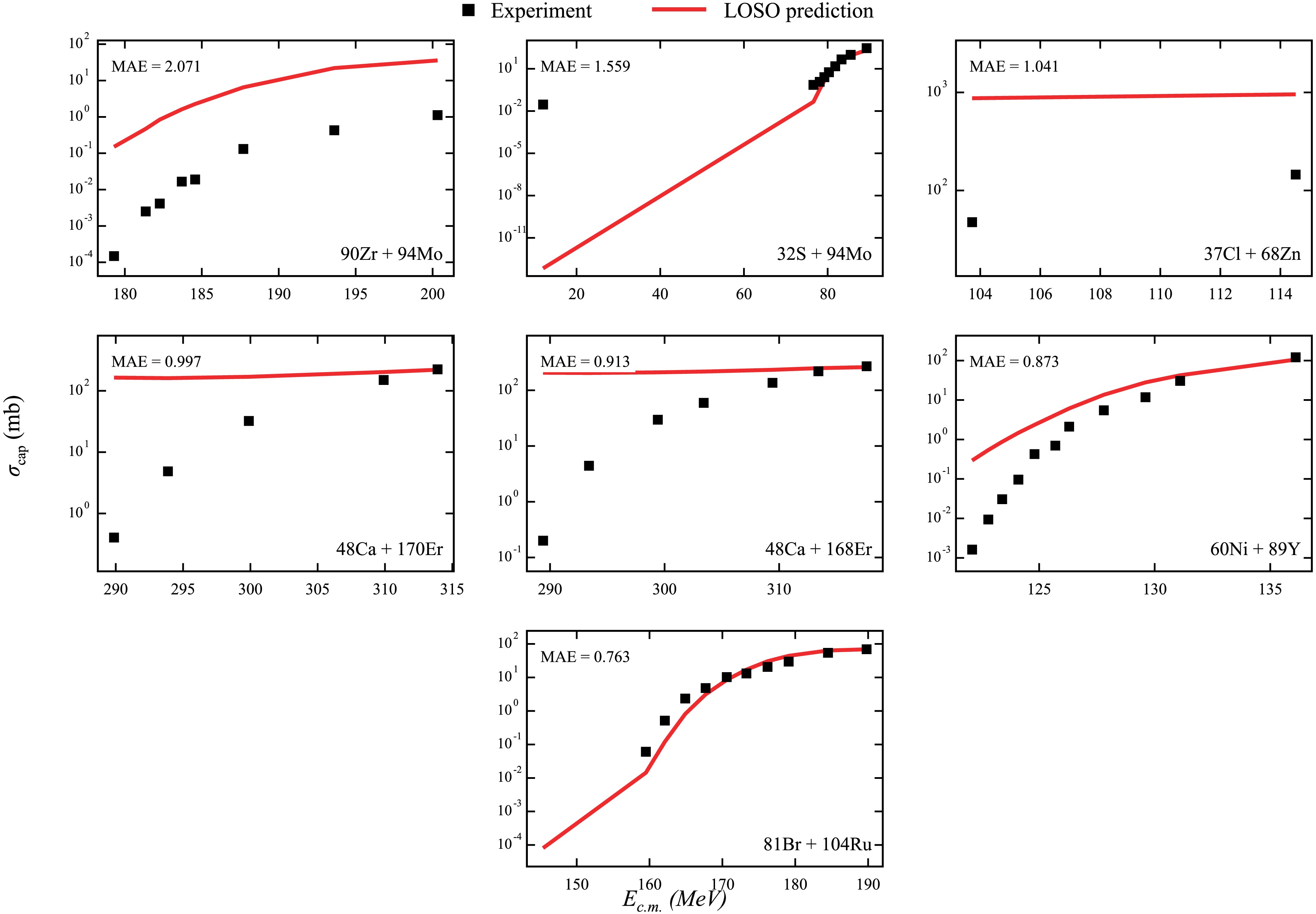

Figure A1.  (color online) Excitation-function comparisons between experimental capture-cross-section data (black solid squares) and TabPFN_S predictions (red solid lines) for the seven high-MAE projectile–target combinations with group-wise $ \overline{\mathrm{MAE}}>0.75 $ from LOSO-CV. These seven systems correspond to Nos. 1–7 listed in Table A1. Each subpanel shows the measured and predicted capture cross sections as a function of the center-of-mass energy $ E_\mathrm{c.m.} $.