


 Abstract
 HTML
 Reference
 Related
 PDF



-
The Schwinger model provides a concise framework for studying confinement, background electric flux, chiral structure, and vacuum-angle dependence using both field-theoretical and nonperturbative methods: the massless theory is exactly solvable and generates a massive gauge boson through the anomaly [1], while the massive theory acquires a nontrivial dependence on the vacuum angle θ [2]. Its multi-flavor extensions introduce flavor dynamics and explicit mass imbalance while retaining a one-dimensional formulation well suited to tensor network calculations [3−7]. The region around
$ \theta=\pi $ is especially subtle because competing vacuum structures and long correlation lengths amplify finite-size and boundary effects.Because the Kogut–Susskind Hamiltonian lattice formulation [8] makes the model directly accessible to real-space variational methods, it has become a standard proving ground for tensor networks in lattice gauge theory. Density-matrix renormalization group (DMRG) calculations resolved the mass spectrum of the one-flavor massive model two decades ago [9], and matrix product state (MPS) formulations that either eliminate the gauge links by Gauss's law or retain them explicitly were developed shortly thereafter [10−12]. This approach has since yielded the chiral condensate at finite lattice spacing [13], the confining string and its breaking [14], density-induced transitions [15], the topological vacuum structure at finite θ [16], the CP-violating Dashen phase [17], and combined analytic and DMRG results on a finite interval [18]; broader accounts of the method and its scope are given in Refs. [19−21]. More recently, gauge-invariant uniform MPS have been used to characterize the critical behavior of the one-flavor model [22].
Quantities computed from the entanglement structure of these states have become observables in their own right. The entanglement entropy of a one-dimensional critical system is controlled by the central charge [23], while the full Schmidt spectrum, or entanglement spectrum, retains structural information that the entropy alone discards [24]. When the state carries a global symmetry, the reduced density matrix decomposes into charge sectors; the sector weights can equivalently be viewed as subsystem-charge probabilities generated by charged moments, thereby linking symmetry-resolved entanglement to full counting statistics [25−27]. This structure has also been shown to be sensitive to open boundaries [28]. In a gauge theory, the subsystem algebra and Hilbert space factorization require an explicit prescription [29], which the superselection-resolved tensor network construction of Ref. [30] supplies for lattice gauge theories. In the Schwinger model itself, entanglement entropy and global entanglement-spectrum spacing have been used to diagnose the one-flavor critical region [31], and finite-θ studies relate entropy enhancement to competition between electric-flux branches [32].
The two-flavor theory provides the flavor structure exploited in the present work. Hetrick, Hosotani, and Iso established the bosonized description of the massive multi-flavor model [3], and Smilga obtained the critical amplitudes that organize its small-mass expansion [33]. Dempsey et al. mapped the zero-temperature phase diagram and identified the role of staggered-lattice charge conjugation at
$ \theta=\pi $ [4], a direction continued in Ref. [7], where the strong-coupling low-energy description at$ \theta=\pi $ is developed in detail. On the numerical side, DMRG has resolved the θ-dependent meson spectrum [34, 35], MPS calculations have determined the additive mass shift of Wilson and staggered fermions [36] and directly compared fermion discretizations [37], Grassmann tensor-renormalization-group calculations have resolved the thermodynamic-limit lattice phase structure with a θ term [6], and lattice Monte Carlo has addressed chiral and isospin breaking [5].The physical question is how the background source, electric self-energies, and interflavor coupling organize charged vacuum fluctuations and determine their flavor composition. We address this question in the two-flavor Schwinger model at
$ \theta=\pi $ through the joint Schmidt probability distribution$ p_{Q_A,F_A} $ . Its marginal$ p_{Q_A} $ records the gauge-charge organization, while$ p_{F_A\mid Q_A} $ resolves the flavor distribution at fixed subsystem charge. For the complementary$ (Q_A,F_A)=(\pm1,\pm1) $ pairs, we distinguish the combined pair weight$ W_F^{(q)} $ from the pair-normalized conditional polarization$ {\cal{P}}_F^{(q)} $ , while independently tracking the gauge-sector identity of the globally leading levels across the two staggered cut classes. These established symmetry-resolved constructions separate the gauge-charge marginal, the$ F_A=\pm1 $ pair weight and flavor asymmetry within a fixed charge sector, and the sector's position in the global Schmidt ordering. We study finite open staggered chains with a matter-site bipartition. This question complements, rather than contradicts, the critical-point diagnostics of Ref. [31].The positive intra-cell
$ {\cal{P}}_F^{(+1)} $ indicates that the heavy flavor carries the more probable positive unit-charge event. To explain this$ \theta=\pi $ result, we trace the same charge statistics from zero background at fixed masses, hopping, and geometry. The actual event probabilities show that the light-flavor contribution is sufficiently suppressed to lose its initial advantage; single-flavor odds and induced flux characterize the accompanying charge rearrangement. Matched controls separate the reversal attainable from the external source alone from the effects of electric self-energies and interflavor coupling on the endpoint and event weights. Interpolations in the background angle and small hopping serve as mechanism probes for the$ \theta=\pi $ flavor preference, while matched average-mass and geometric comparisons test its parameter dependence. The mechanism is encoded in these charge probabilities, or joint full counting statistics, rather than in a newly resolved internal structure of the normalized entanglement blocks.We find that changing the staggered cut class switches the dominant non-neutral Schmidt pair from
$ Q_A=-1 $ at unit-cell boundaries to the complementary$ Q_A=+1 $ pair at intra-cell cuts. Mass imbalance drives both$ {\cal{P}}_F^{(-1)} $ and$ {\cal{P}}_F^{(+1)} $ away from zero with a charge- and cut-dependent response: at unequal mass,$ {\cal{P}}_F^{(-1)} $ is positive for both cut classes, whereas$ {\cal{P}}_F^{(+1)} $ is negative at unit-cell boundaries and positive intra-cell. Within the tracked$ Q_A=-1 $ pair, increasing the mass ratio along the fixed geometric-mean path also increases its combined probability, even though the intra-cell pair weight is strongly suppressed relative to the unit-cell value. The complete joint distribution further distinguishes non-neutral broadening at unit-cell boundaries from redistribution among non-neutral sectors at intra-cell cuts. We establish these results using matrix product state calculations validated by exact diagonalization and symmetry-resolved Schmidt decompositions.This paper is organized as follows. Section II introduces the lattice formulation, subsystem quantum numbers, Schmidt sector probabilities, and numerical methods. Section III presents the cut-dependent gauge-sector ordering, joint probability distribution, flavor-pair response, and its background-field origin. Section IV discusses the physical content and scope, and Sec. V summarizes the results. Atomic reference selection rules, logarithmic probability relations, convergence checks, and targeted parameter controls are provided in the Appendix, while the availability of the underlying datasets is stated in the Data availability statement.
-
Detailed accounts of the Hamiltonian lattice formulation and its matrix product state implementation can be found in Refs. [8, 10, 38]. Here, we reproduce only the conventions required for the subsequent analysis and then specify the numerical settings in full.
-
We use the Kogut–Susskind Hamiltonian lattice formulation [8] for a two-flavor Schwinger model with
$N_s$ matter sites. The matter sites are indexed by$n=0,\ldots,N_s-1$ , and each physical site contains two fermionic modes labeled by$\alpha=1,2$ . The gauge field is eliminated using Gauss's law under open boundary conditions. The dimensionless bare flux$ L_n $ is associated with the link connecting sites$ n $ and$ n+1 $ , and the physical electric field is$ E_n=g[L_n+\theta/(2\pi)] $ . We fix a bare link flux$L_{-1}$ to the left of the chain and reconstruct the internal electric fields using Eq. (1):$ L_n-L_{n-1}=Q_n, \qquad L_n=L_{-1}+\sum\limits_{k=0}^{n}Q_k. $
(1) Equations (3)–(6) define the Hamiltonian used in the three numerical representations. The Hamiltonian includes the
$N_s-1$ internal dynamical links,$n=0,\ldots,N_s-2$ . The right external flux is fixed by the total charge,$ L_{\mathrm{right}} = L_{-1}+Q_{\mathrm{tot}}, $
(2) but its energy is not included in the Hamiltonian used to obtain the quantitative results. This distinction is relevant outside a fixed total-charge sector. The internal-link convention is used throughout this work.
The Hamiltonian is decomposed as
$ H=H_{\mathrm{hop}}+H_{\mathrm{mass}}+H_E. $
(3) $ H_{\mathrm{hop}} = -\frac{i}{2a} \sum\limits_{n=0}^{N_s-2}\sum\limits_{\alpha=1}^{2} \left( c^\dagger_{n,\alpha}c_{n+1,\alpha} - c^\dagger_{n+1,\alpha}c_{n,\alpha} \right), $
(4) $ H_{\mathrm{mass}} = \sum\limits_{n=0}^{N_s-1}\sum\limits_{\alpha=1}^{2} m_{\mathrm{lat},\alpha}(-1)^n n_{n,\alpha}, \qquad m_{\mathrm{lat},\alpha} = m_\alpha-\frac{g^2a}{4}, $
(5) and
$ H_E = \frac{g^2a}{2} \sum\limits_{n=0}^{N_s-2} \left[ L_{-1} +\sum\limits_{k=0}^{n}Q_k +\frac{\theta}{2\pi} \right]^2. $
(6) The three terms represent nearest-neighbor fermion hopping, staggered mass energy, and electric-field energy, respectively. The local gauge charge appearing in Eq. (1), including the staggered background contributions from both flavors, is
$ Q_n = \sum\limits_{\alpha=1}^{2} \left[ n_{n,\alpha} - \frac{1-(-1)^n}{2} \right] = n_{n,1}+n_{n,2}-\left[1-(-1)^n\right]. $
(7) The definition in Eq. (7) includes the staggered background. The background angle shifts the electric energy but does not enter Gauss's law or
$Q_n$ . The total conserved quantum numbers specifying the canonical sector are$ Q_{\mathrm{tot}}=\sum\limits_{n=0}^{N_s-1}Q_n, \qquad F_{\mathrm{tot}}=\sum\limits_{n=0}^{N_s-1}(n_{n,1}-n_{n,2}). $
(8) We use
$g$ as the unit of mass and energy, setting$g=1$ . The mass, cut-class, and geometric comparisons use$ \theta=\pi,\qquad L_{-1}=0, $
(9) with all other parameters held fixed as the auxiliary-mechanism scan varies θ over
$ 0\leq\theta\leq\pi $ . The small-hopping probe replaces$ H_{\rm{hop}} $ with$ hH_{\rm{hop}} $ , with$ h=1 $ restoring the Hamiltonian above; neither probe recomputes the lattice mass shift. Throughout, the MPS is restricted to$ Q_{\mathrm{tot}}=0, \qquad F_{\mathrm{tot}}=0. $
(10) We work in the zero-charge, flavor-neutral canonical sector. Each response MPS is the lowest-energy state obtained in this sector and satisfies the criteria in Sec. II.E.2. The exact symmetry maps in Appendix D.3 provide additional checks of the sector construction. Staggered-lattice charge conjugation also translates matter and links by one site, schematically
$ c_{n,\alpha}\mapsto c^\dagger_{n+1,\alpha} $ and$ L_n\mapsto-L_{n+1}-1 $ at$ \theta=\pi $ [4]. The choice$ L_{-1}=0 $ , together with the open termination and the convention for internal-link electric energy, therefore defines a finite-chain realization that is not invariant under the staggered charge-conjugation transformation. In the C-broken region of the infinite-volume phase diagram, this boundary condition removes the finite-system equivalence of the two C-related bulk vacua and selects one finite-chain continuation. We do not infer the vacuum degeneracy of the thermodynamic system from this selection.The dimensionless lattice parameter is
$ x=\frac{1}{g^2a^2}. $
(11) The gauge-covariant staggered Hamiltonians of Refs. [4, 7] use the same imaginary, antisymmetric hopping terms, Gauss-law charge, and two-flavor mass shift; the latter has also been determined using MPS methods [36]. On the open chain, we set the link phases to
$ U_n=1 $ and adopt the internal link-endpoint convention of the gauge-eliminated OBC formulation [10]. The operator-independent constant in the shifted electric-field squares is retained, whereas the staggered background is already included in$ Q_n $ . Appendix A.1 provides the exact rearrangement of the electric term and the corresponding MPO coefficients. -
The local Hilbert space is four-dimensional. We use
$ |n_1,n_2\rangle = |0,0\rangle,\ |1,0\rangle,\ |0,1\rangle,\ |1,1\rangle. $
(12) The intrasite fermionic sign is chosen so that the two local flavors satisfy the canonical anticommutation relations. The full-chain mode ordering is site-major.
$ (0,1),(0,2),(1,1),(1,2),\ldots,(N_s-1,1),(N_s-1,2). $
(13) Cross-site operators use the corresponding Jordan–Wigner strings, with identical site-major ordering in the ED and tensor-network implementations.
-
For a bipartition after the first
$\ell$ physical sites, the left subsystem is$ A=\{0,\ldots,\ell-1\}. $
(14) We define
$ N_{1,A}=\sum\limits_{n<\ell}n_{n,1}, \qquad N_{2,A}=\sum\limits_{n<\ell}n_{n,2}, $
(15) with
$ N_A=N_{1,A}+N_{2,A}, $
(16) and the integer flavor imbalance
$ F_A=N_{1,A}-N_{2,A}. $
(17) The physical subsystem gauge charge is
$ Q_A=\sum\limits_{n<\ell}Q_n. $
(18) The staggered background contribution is included in
$Q_A$ , so$Q_A$ cannot be replaced by the bare occupation number. Gauss's law yields$L_{\ell-1}=L_{-1}+Q_A$ . Thus,$Q_A$ labels the electric-flux superselection sector across the cut, whereas$F_A$ further resolves the conserved flavor-$U(1)$ block [30]. In terms of the subsystem occupation number,$ Q_A=N_A-2\left\lfloor\frac{\ell}{2}\right\rfloor. $
(19) Appendix A.2 presents the tensor-network label mapping and its ED validation. The flavor-resolved net charges are
$\begin{aligned}[b]& Q_{1,A}=N_{1,A}-\left\lfloor\frac{\ell}{2}\right\rfloor =\frac{Q_A+F_A}{2},\\& Q_{2,A}=N_{2,A}-\left\lfloor\frac{\ell}{2}\right\rfloor =\frac{Q_A-F_A}{2}.\end{aligned} $
(20) For
$ m_1>m_2 $ , an event with$ q=+1,F_A=+1 $ has$ (Q_{1,A},Q_{2,A})=(1,0) $ and carries a positive net charge in the heavy flavor, whereas an event with$ q=-1,F_A=+1 $ has$ (0,-1) $ and carries a negative net charge in the light flavor. These are subsystem net-charge assignments, not single-particle descriptions of the complete many-body state. -
The bipartition is not neutral with respect to the staggered structure; the following classification is used throughout the analysis. Under the chosen staggered convention, two adjacent matter sites form a natural unit cell.
$ (2j,2j+1). $
(21) A cut
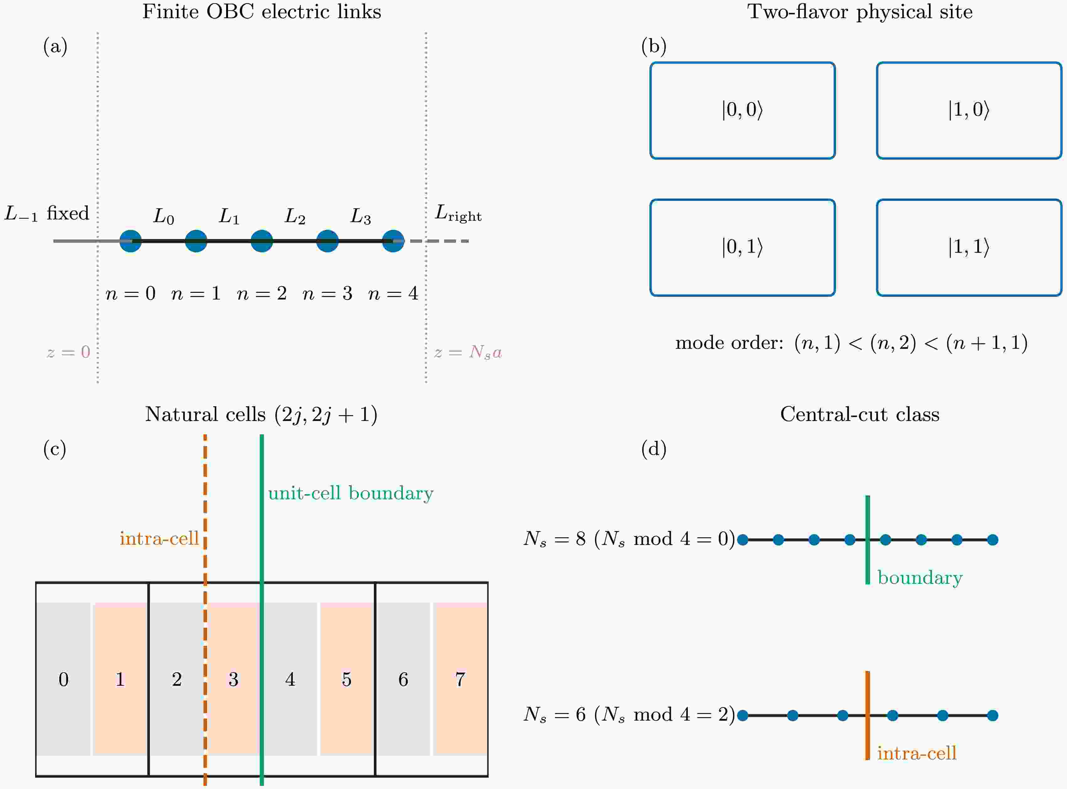
$\ell$ is defined between sites$\ell-1$ and$\ell$ . Cuts with odd and even$\ell$ belong to different bond classes: one lies within the staggered unit cell, whereas the other lies between complete unit cells. For a chain with even$N_s$ ,$N_s\text{mod}4$ determines the class of the central cut. The central cut is a unit-cell boundary for$N_s\text{mod}4=0$ and an intra-cell cut for$N_s\text{mod}4=2$ . The deterministic rule used to select the analysis cut from the available unit-cell boundaries is provided in Appendix B.5.Figure 1 summarizes the boundary, local-basis, fermionic-ordering, and cut conventions used below.
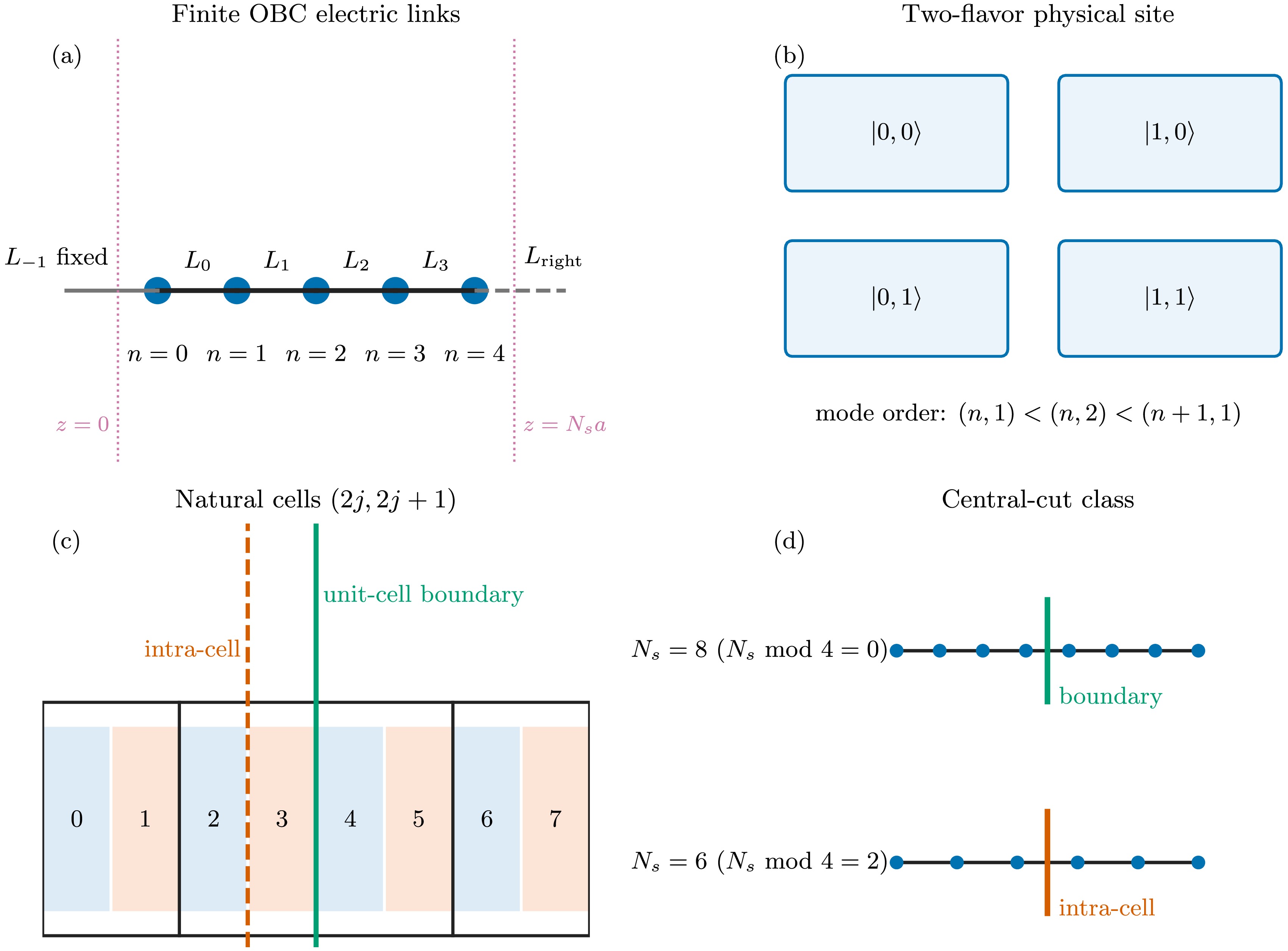
Figure 1. (color online) We use the open-boundary link convention, the four-state two-flavor local basis, site-major fermion ordering, the natural staggered unit cell
$ (2j,2j+1) $ , and the intra-cell and unit-cell-boundary cut classes. Here,$ n $ ,$ j $ , and$ \ell $ are integer lattice indices;$ a $ is the lattice spacing; and$ z $ is a length coordinate, with the chain endpoints at 0 and$ N_sa $ . -
In this subsection, the mass path and its bulk-phase classification refer to
$ \theta=\pi $ . The background-angle mechanism probe follows a separate fixed-mass path.We fix the geometric mean mass and vary the ratio
$ m_{\mathrm{geom}}=\sqrt{m_1m_2}, \qquad r=\frac{m_1}{m_2}, $
(22) so that
$ m_1=m_{\mathrm{geom}}\sqrt r, \qquad m_2=\frac{m_{\mathrm{geom}}}{\sqrt r}. $
(23) The main parameter grid uses
$m_{\mathrm{geom}}/g=0.5$ and$1\le r\le2$ , spanning equal and nondegenerate masses. Along this path,$m_1/g$ ranges from 0.5 to 0.707, and$m_2/g$ ranges from 0.5 to 0.354, resolving the response to mass imbalance without introducing an extreme hierarchy. The geometric-mean constraint also enables exact reciprocity checks, because exchanging the two flavor labels maps$r$ to$\frac{1}{r}$ . According to the zero-temperature phase diagram of Ref. [4], the sampled path$ m_{\mathrm{geom}}/g=0.5 $ ,$ 1\le r\le2 $ , lies within the region where charge conjugation C is spontaneously broken in the infinite-volume theory. The equal-mass point lies on the$ SU(2) $ -invariant line within this region, whereas increasing r moves the path toward the Ising boundary without reaching it over the interval studied here. The selected interval therefore probes flavor imbalance within a single bulk phase rather than crossing a phase boundary, and it does not constitute a pure flavor-breaking susceptibility path. Thus, a flavor-invariant observable must obey$ O(r)=O \left(\frac{1}{r}\right). $
(24) It is useful to introduce
$ \eta=\ln r. $
(25) The parameterization in Eq. (22) makes flavor exchange correspond to
$\eta\rightarrow -\eta$ .At equal masses, the continuum theory has an
$ SU(2)/\mathbb Z_2\simeq SO(3) $ flavor symmetry. Writing the real mass matrix as$ \widetilde M=m\mathbb I_2+\delta m\,\sigma^3 $ gives$ m=m_{\rm{geom}}\cosh \left(\frac{\eta}{2}\right), \qquad \delta m=m_{\rm{geom}}\sinh \left(\frac{\eta}{2}\right), \qquad \eta=\ln r, $
(26) Thus, flavor-invariant and flavor-odd responses are even and odd in η, respectively [3−5, 7, 33].
Along the geometric-mean path, both the average mass and the mass difference vary. Matched equal-mass references are used to separate their finite-difference contributions in Appendix E.2.
-
Across a physical-site cut, the MPS Schmidt singular values
$ s_\alpha $ define the probabilities and entanglement energies.$ \lambda_\alpha=s_\alpha^2, \qquad \epsilon_\alpha=-\ln\lambda_\alpha. $
(27) A fixed total charge and flavor imbalance render the reduced state block diagonal in
$ (Q_A,F_A) $ , yielding the normalized direct-sum decomposition$ \rho_A=\bigoplus\limits_{Q_A,F_A}p_{Q_A,F_A}\,\widetilde\rho_{Q_A,F_A}, \qquad \text{Tr}\widetilde\rho_{Q_A,F_A}=1, $
(28) where
$ p_{q,f}\equiv p_{Q_A=q,F_A=f}=\text{Tr}\rho_A^{(q,f)} $ denotes the total Schmidt probability of the block labeled by$ (q,f) $ .Because flavor exchange is an on-site internal unitary, it factorizes across any physical-site bipartition as
$ {\cal{X}}={\cal{X}}_A\otimes{\cal{X}}_{\bar A} $ . It therefore preserves the Schmidt values while mapping$ F_A\to-F_A $ . The block rank k orders the density-matrix eigenvalues from largest to smallest, equivalently the entanglement energies from lowest to highest, within a given$ (Q_A,F_A) $ block. For ground states related by the corresponding exchange, at fixed k,$ \epsilon_k^{(Q_A,F_A)}(r)=\epsilon_k^{(Q_A,-F_A)} \left(\frac{1}{r}\right). $
(29) Equivalently,
$ p_{q,f}=\langle\Psi|\Pi^A_{q,f}|\Psi\rangle, $
(30) These block weights constitute the joint full counting statistics of the subsystem flavor charges, expressed in terms of the equivalent labels
$ Q_A $ and$ F_A $ . We denote the gauge-charge marginal by$ p_{Q_A}(q)\equiv\sum\nolimits_f p_{q,f} $ and, when$ p_{Q_A}(q)>0 $ , the conditional flavor distribution by$ p_{F_A\mid Q_A}(f\mid q)\equiv p_{q,f}/p_{Q_A}(q) $ . For the complementary flavor pairs with$ q=\pm1 $ , define$ W_F^{(q)}=p_{q,+1}+p_{q,-1}, \qquad {\cal{P}}_F^{(q)} =\frac{p_{q,+1}-p_{q,-1}}{p_{q,+1}+p_{q,-1}}, \qquad q=\pm1. $
(31) Here,
$ W_F^{(q)} $ denotes the total joint probability associated with the$ F_A=\pm1 $ pair within charge sector q. Because the common marginal factor cancels,$ {\cal{P}}_F^{(q)} $ is equivalently the normalized contrast of$ p_{F_A\mid Q_A}(\pm1\mid q) $ ; when other flavor values are present, however, it is not the first moment of the complete conditional distribution. For the$ q=-1 $ pair, we further write$ p_+\equiv p_{-1,+1}, \qquad p_-\equiv p_{-1,-1}. $
(32) The logarithmic entanglement-level difference
$ D_F $ essentially reparameterizes the same conditional-probability asymmetry and is discussed in Appendix D.Flavor exchange imposes exact parity constraints. With
$ \eta=\ln r $ ,$ W_F^{(q)}(\eta)=W_F^{(q)}(-\eta), \qquad {\cal{P}}_F^{(q)}(\eta)=-{\cal{P}}_F^{(q)}(-\eta), \qquad q=\pm1. $
(33) In particular,
$ \left.{\cal{P}}_F^{(q)}\right|_{r=1}=0 $ in the equal-mass case. These constraints determine neither the nonzero magnitude nor the cut dependence. The probabilities, polarizations, entanglement energies, and their differences are dimensionless; the entanglement energy is not a physical excitation energy rendered dimensionless by setting$ g=1 $ . Throughout,$ \ln $ denotes the natural logarithm.For these two commuting labels, we define
$ Z_{n,A}(\alpha,\beta) =\text{Tr} \left[\rho_A^n e^{i\alpha Q_A+i\beta F_A}\right], \qquad n=1,2,\ldots . $
(34) Here
$ n $ is the order of the moment. At$ n=1 $ ,$ Z_{1,A} $ is the standard joint characteristic function, and its Fourier coefficients are$ p_{q,f} $ ; higher-order charged moments generate symmetry-resolved Rényi moments. This is the two-charge extension of the charged-moment/full-counting-statistics construction used in symmetry-resolved entanglement [25−27]; the Schmidt decomposition additionally provides the normalized spectrum within each block.The normalization of the complete Schmidt spectrum is checked before applying any low-lying-level filtering. All joint block probabilities
$ p_{q,f} $ used here are summed over every Schmidt value present in the available MPS state. The threshold$ \lambda_\alpha>10^{-12} $ is applied only to low-lying-level tables and dominant-block identification; it is not applied to the block-weight reconstruction. Symmetry-resolved entanglement decompositions have been developed in continuum and lattice settings [26, 27]. In gauge theories, the subsystem algebra and Hilbert-space factorization require an explicit prescription [29]; here, the gauge links have first been eliminated by the Gauss law, and the Schmidt cut is taken only between complete matter sites. -
Sparse ED provides the reference for small systems. The mass and electric diagonal entries use the same local charge and Gauss-law definitions as those used in the tensor network construction; no independent boundary convention is introduced. The lowest eigenpairs are obtained with a sparse Hermitian eigensolver. Technical details, including explicit basis maps and the fallback for very small matrices, are summarized in Appendix B.
After summing over internal links, the site-dependent one-body terms and long-range two-body terms admit an exact finite-state MPO representation without requiring an approximate long-range fit. The construction and bond dimensions are given in Appendix A.1.
-
We use TeNPy 1.1.0 [39, 40] with one four-state MPS site for each physical matter site. The backend conserves the Abelian charge pair
$(N,F)$ , which is mapped to the physical subsystem labels$(Q_A,F_A)$ , as described in Sec. II.B.2. The physical Hilbert basis and Hamiltonian are unchanged when these symmetries are enabled.Finite-system DMRG [38, 41] targets the lowest-energy state in the fixed neutral canonical sector. Energy, the Schmidt spectrum, local observables, and discarded weight are compared between successive bond dimensions; the convergence criteria and component-wise tests are given in Appendices B.4 and E.1.
-
We use
$g$ as the unit for both mass and energy. The primary mass-grid parameters are$ \theta=\pi,\qquad m_{\mathrm{geom}}/g=0.5. $
(35) The combined data set comprises
$ x=4,6.25,9,12.25 $ and a scan over six ratios,$ r=1,1.125,1.25,1.5,1.75,2 $ , at$ gL_{\mathrm{phys}}\simeq8 $ . We express the physical spatial length as$ L_{\mathrm{phys}}=N_s a, \qquad gL_{\mathrm{phys}}=\frac{N_s}{\sqrt{x}}. $
(36) We place matter site
$n$ at$z_n=\left(n+\frac{1}{2}\right)a$ , between the geometric boundaries at$z=0$ and$z=N_sa$ ; Appendix A.3 provides the full coordinate convention.The six-ratio scan at
$ gL_{\rm{phys}}=8 $ is supplemented by targeted length comparisons at$ r=1,1.5,2 $ , rather than by a complete Cartesian grid. Table 1 lists the actual lengths and final bond dimensions.Subset x $ N_s $ $ gL_{\mathrm{phys}} $ Mass ratios χ $ \ell_\star $ $ gL_{\mathrm{phys}}\simeq8 $ scan4 16 8.00 $ 1,1.125,1.25,1.5,1.75,2 $ 256 8 6.25 20 8.00 same 256 10 9 24 8.00 same 256 12 12.25 28 8.00 same 256 14 $ gL_{\mathrm{phys}}\simeq10 $ checks4 20 10.00 $ 1,1.5,2 $ 256 10 6.25 24 9.60 same 256 12 9 28 9.33 same 256 14 12.25 36 10.29 same 384 18 $ gL_{\mathrm{phys}}\simeq12 $ checks9 36 12.00 $ 1,1.5,2 $ 256 18 12.25 40 11.43 same 384 20 Table 1. Parameter coverage for the relative-response analysis is as follows. Each listed analysis cut corresponds to the central unit-cell boundary, and all systems satisfy
$ N_s\text{mod}4=0 $ . The$ gL_{\mathrm{phys}}\simeq10,12 $ and near-equal calculations are targeted checks rather than a complete Cartesian scan. Matched$ r=1 $ references are shared when the numerical parameters coincide. Here, x, r,$ gL_{\mathrm{phys}} $ , and χ are dimensionless;$ N_s $ denotes the number of matter sites, and$ \ell_\star $ is an integer cut index.The background-field probe uses
$ (x,N_s,r)=(4,16,2) $ and the targeted extensions$ (4,20,2) $ and$ (4,16,1.5) $ , varying only θ while keeping the masses, hopping, and geometry fixed. Appendix E reports their coverage, omitted weights, and final-state precision. -
We first establish the organization of charge sectors and the heavy-flavor preference at
$ \theta=\pi $ ; we then use the background-field response to explain how this preference emerges. -
The two staggered cut classes are also evident in the alternating entropy and global-gap profiles (Appendix B.2). The resolved gauge-sector ordering below provides a direct spectral distinction between them.
The unresolved spectrum is obtained by sorting all retained entanglement levels
$ \epsilon_\alpha $ irrespective of symmetry. Its first spacing,$ \Delta_\epsilon^{\mathrm{global}}=\epsilon_2-\epsilon_1, $
(37) may therefore compare different
$ (Q_A,F_A) $ blocks. This inter-flux spacing is well defined, but it is not an internal spacing within either block. Under the$ L_{-1}=0 $ ,$ \theta=\pi $ convention,$ Q_A=0,-1,+1 $ correspond, respectively, to shifted cut fluxes$ +1/2,-1/2,+3/2 $ .Across the primary mass grid, the first two global levels at the selected complete-unit-cell boundaries lie in
$ Q_A=0 $ and$ Q_A=-1 $ , whereas each reflection-related pair of adjacent intra-cell cuts gives$ Q_A=0\leftrightarrow+1 $ . The$ Q_A=-1,F_A=\pm1 $ partner minima remain identifiable, shifting from ranks 2 and 3 at the selected boundary to ranks 4 and 5–7 within the cell. Thus, global Schmidt-level sorting and the fixed-sector flavor response carry different information. Figure 2 illustrates the resolved spectra for one representative state.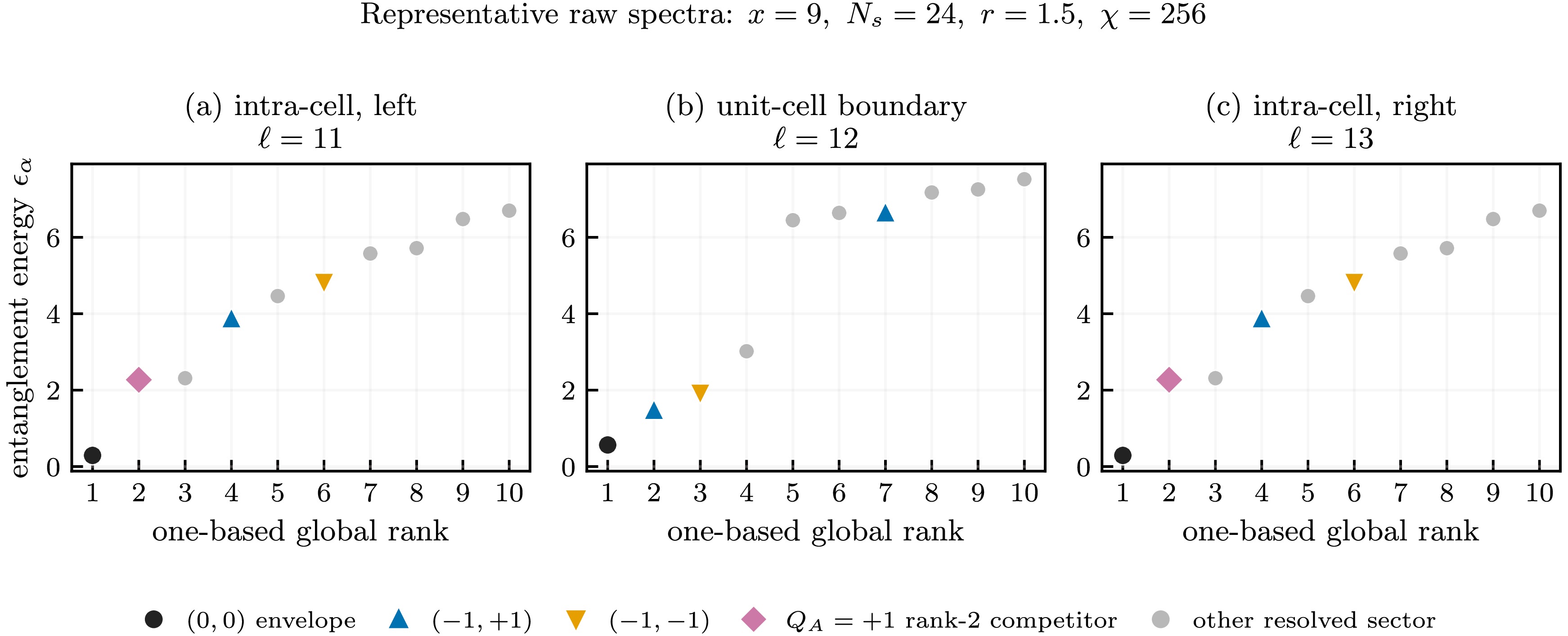
Figure 2. (color online) Representative low-lying entanglement spectra for the state with
$ x=9 $ ,$ N_s=24 $ ,$ r=1.5 $ , and$ \chi=256 $ at (a) the left adjacent intra-cell cut, (b) the selected unit-cell boundary, and (c) the right adjacent intra-cell cut. Each panel shows the first ten global levels on identical axes. The selected boundary exhibits the leading$ Q_A=0\leftrightarrow-1 $ pair, whereas both adjacent cuts exhibit$ Q_A=0\leftrightarrow+1 $ ; the tracked$ Q_A=-1,F_A=\pm1 $ levels remain identifiable at higher ranks. Entanglement energies are dimensionless, and global rank is an ordinal index. -
The complete Schmidt distribution resolves a complementary pair in the
$ Q_A=+1 $ sector, in addition to the tracked$ Q_A=-1 $ pair. Applying Eq. (31) to both$ q=\pm1 $ sectors shows that both partner blocks have nonzero probability at each analyzed primary cut. The probability outside the$ F_A=\pm1 $ pair is quantified in Appendix E.1. The full gauge-charge marginals$ p_{Q_A}(\pm1) $ follow the same cut-dependent ordering as the complementary-pair weights. This ordering undergoes a complete reversal:$\begin{aligned}[b]& W_F^{(-1)}>W_F^{(+1)} \quad\text{at unit-cell boundaries},\\& W_F^{(+1)}>W_F^{(-1)} \quad\text{intra-cell}. \end{aligned}$
(38) Thus, the
$ Q_A=-1 $ pair dominates at every selected unit-cell boundary, whereas the$ Q_A=+1 $ pair dominates for every reflection-related intra-cell pair. Together with the global-rank identities in Sec. III.A, this result confirms the complementary pair switch. The corresponding conditional polarizations are not mirror copies: for unequal masses,$ {\cal{P}}_F^{(+1)} $ is negative at unit-cell boundaries and positive at intra-cell cuts, whereas$ {\cal{P}}_F^{(-1)} $ is positive at both types of cuts.Figure 3 shows the changes in the dominant joint probability components relative to the equal-mass state at fixed
$ gL_{\mathrm{phys}}=8 $ . At unit-cell boundaries,$ \Delta W_F^{(-1)} $ closely tracks the positive change in the total non-neutral probability, whereas the$ Q_A=+1 $ pair changes only weakly. At intra-cell cuts,$ \Delta W_F^{(-1)}>0 $ occurs together with a larger decrease in$ W_F^{(+1)} $ and a net reduction in the non-neutral probability. The former response therefore reflects non-neutral broadening dominated by the$ Q_A=-1 $ pair, whereas the latter is primarily a redistribution from the dominant$ Q_A=+1 $ pair toward$ Q_A=-1 $ . These sign patterns hold at all four sampled spacings. The corresponding absolute joint distributions are shown in Appendix B, Fig. B1.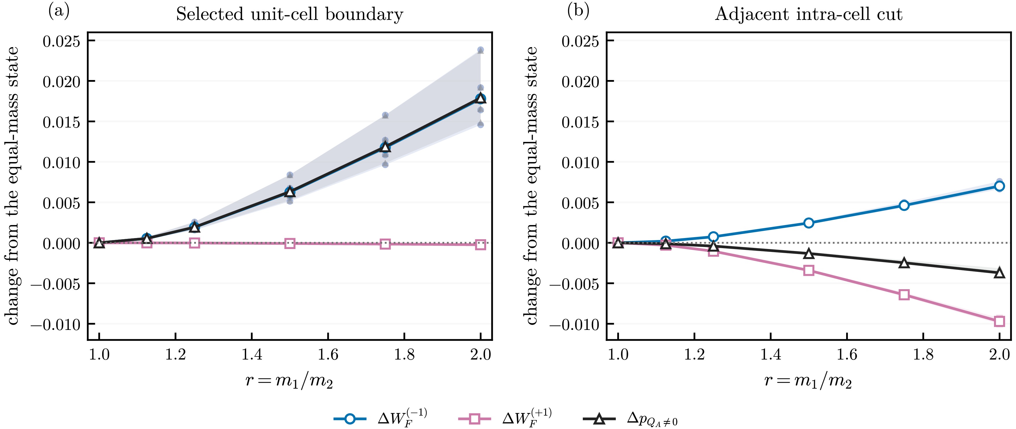
Figure 3. (color online) Reference-subtracted reorganization of the joint Schmidt probability distribution at
$ gL_{\mathrm{phys}}=8 $ . Panel (a) shows the selected unit-cell boundary, and panel (b) shows the mirror-combined adjacent intra-cell cut class. The plotted quantities are changes relative to the equal-mass state at the same x: the two complementary pair weights and the total non-neutral probability,$ p_{Q_A\ne0}=1-p_{Q_A=0} $ . Lines indicate the pointwise median over$ x=4,6.25,9,12.25 $ ; shaded envelopes indicate the deterministic minimum–maximum range; and faint markers indicate all four values. The envelopes describe lattice-spacing dependence and do not represent statistical uncertainties. All plotted quantities, as well as x, r, and$ gL_{\mathrm{phys}} $ , are dimensionless. -
The complete Schmidt vectors provide
$ p_+ $ and$ p_- $ directly, without the need to reconstruct either quantity from a truncated list of leading levels. At every sampled geometry and for each cut class, increasing r yields$ p_+\uparrow, \qquad p_-\downarrow, \qquad W_F^{(-1)}\uparrow, \qquad {\cal{P}}_F^{(-1)}\uparrow $
(39) at the sampled ratios. The simultaneous increases in
$ W_F^{(-1)} $ and$ {\cal{P}}_F^{(-1)} $ are important: along this mass path, the partner pair becomes more probable, and its conditional distribution is biased toward$ F_A=+1 $ . This behavior is not simply a transfer of a fixed amount of probability from$ p_- $ to$ p_+ $ .Compared with the unit-cell boundary, the intra-cell
$ q=-1 $ pair has lower probability but stronger conditional polarization. The detailed cross-cut ratios and their mass dependence are provided in Appendix D.2; the reversed-centering checks in Appendix B.5 confirm that this contrast is determined by the cut class rather than by the one-site centering offset. -
Figure 4 displays the two signed polarizations explicitly. In all 32 unequal-mass primary states,
$ q=-1 $ is positively polarized in both cut classes, whereas$ q=+1 $ has negative polarization at unit-cell boundaries and positive polarization within cells. By Eq. (20), the latter positive sign indicates that the heavy flavor carries the more probable positive unit-charge event. This does not imply a change in the ordering of the input masses.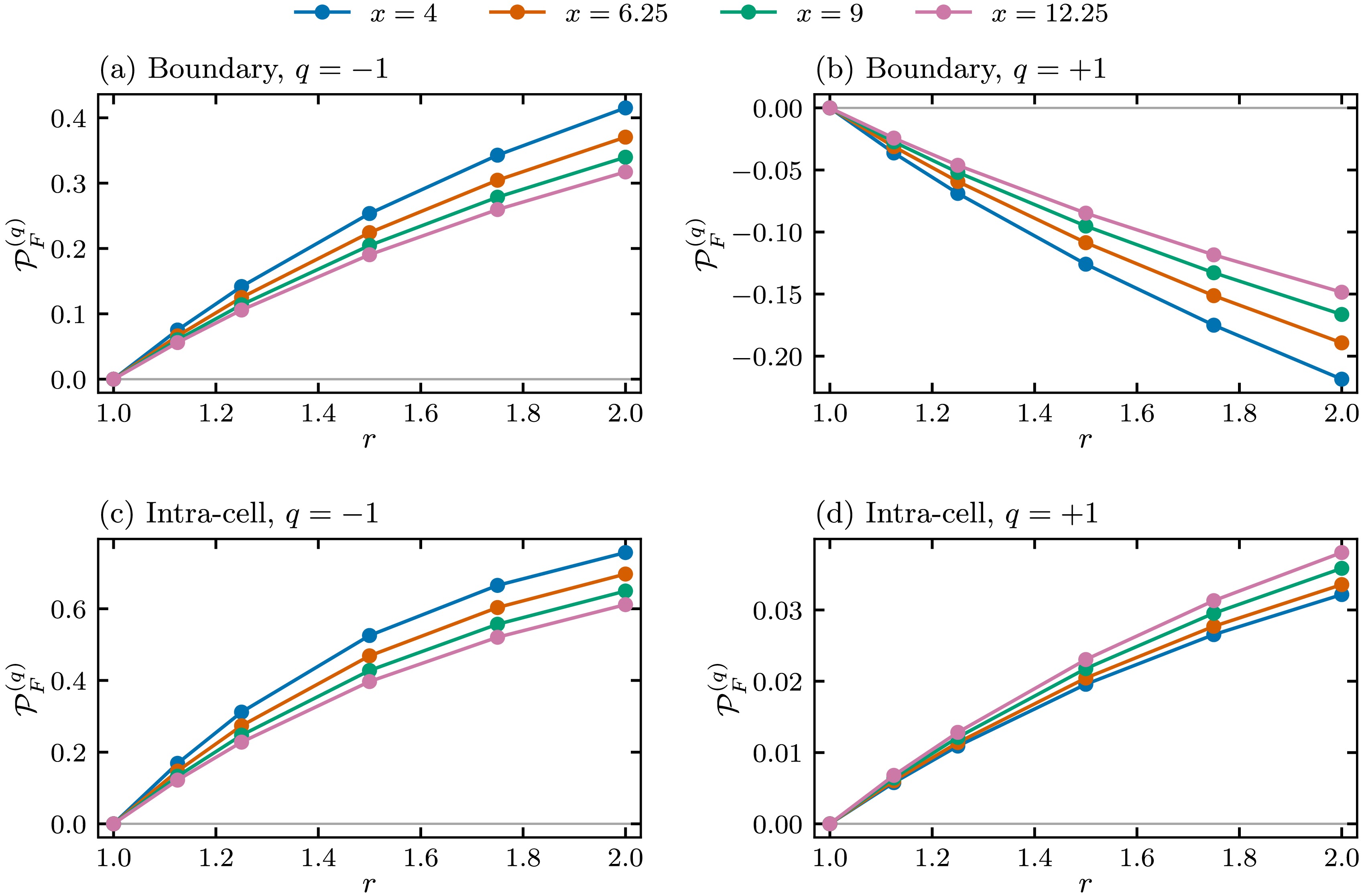
Figure 4. (color online) Signed flavor polarization at
$ \theta=\pi $ ,$ h=1 $ ,$ m_{\rm{geom}}/g=0.5 $ , and$ gL_{\rm{phys}}=8 $ . Columns distinguish$ q=-1 $ and$ q=+1 $ , and rows distinguish the selected unit-cell boundary from the mirror-combined intra-cell cuts. Colors indicate x; all six mass ratios are shown. For positive charge, positive polarization denotes a preference for the heavy flavor; for negative charge, it denotes a preference for the light flavor. All plotted quantities are dimensionless. Componentwise precision is given in Table E1.The sign contrast persists across the range of spacings and lengths considered. At fixed
$ x=4 $ and$ r=2 $ , increasing$ gL_{\rm{phys}} $ from 8 to 10 increases the intra-cell$ {\cal{P}}_F^{(+1)} $ from approximately$ 0.032 $ to$ 0.064 $ . The sign also persists under lattice refinement and reversed centering, whereas its magnitude retains appreciable length dependence. Appendix E.3 separates the spacing and length comparisons.This heavy-flavor preference is opposite to the controlled small-hopping prediction. For the representative
$ x=4,N_s=16,r=2 $ state, the intra-cell$ q=+1 $ polarization approaches$ -0.502909 $ as$ h\to0^+ $ but equals$ +0.032165 $ at$ h=1 $ . The unit-boundary$ q=-1 $ value also receives a substantial correction, from$ +0.732863 $ to$ +0.415256 $ , without changing sign. The next subsection explains the origin of the$ \theta=\pi $ preference by varying the background source while keeping the masses, hopping, and geometry fixed. -
We track the representative state at
$ x=4 $ ,$ N_s=16 $ ,$ r=2 $ ,$ m_{\rm{geom}}/g=0.5 $ , and$ h=1 $ as θ varies from 0 to π. The lattice masses and hopping parameter remain fixed. The chosen boundary is$ \ell=8 $ , and the displayed intra-cell cut is$ \ell=7 $ . In the neutral$ L_{-1}=0 $ realization, Eq. (6) gives$ \begin{aligned}[b] H(\theta)-H(0) =\;& -E_{\rm{bg}}D+(N_s-1)K b^2\mathbf1,\\ E_{\rm{bg}} =\;&\frac{g\theta}{2\pi},\qquad D=ga\sum\limits_k kQ_k,\\ K=\;&\frac{g^2a}{2},\qquad b=\frac{\theta}{2\pi}. \end{aligned} $
(40) Here,
$ \sum\nolimits_nL_n=-\sum\nolimits_k kQ_k $ follows from$ Q_{\rm{tot}}=0 $ . Thus, the angle controls a source conjugate to charge displacement while leaving the other Hamiltonian parameters unchanged.Figure 5(a,b) shows how the heavy-flavor endpoint develops. Both positive charge contributions decrease as the background varies from zero to π, but the light-flavor contribution is suppressed by approximately
$ 50$ %, compared with$ 20$ % for the heavy flavor. This unequal suppression overcomes the initial light-flavor advantage:$ {\cal{P}}_F^{(+1)} $ changes from approximately$ -0.203 $ to$ +0.032 $ . The measured opposite signs give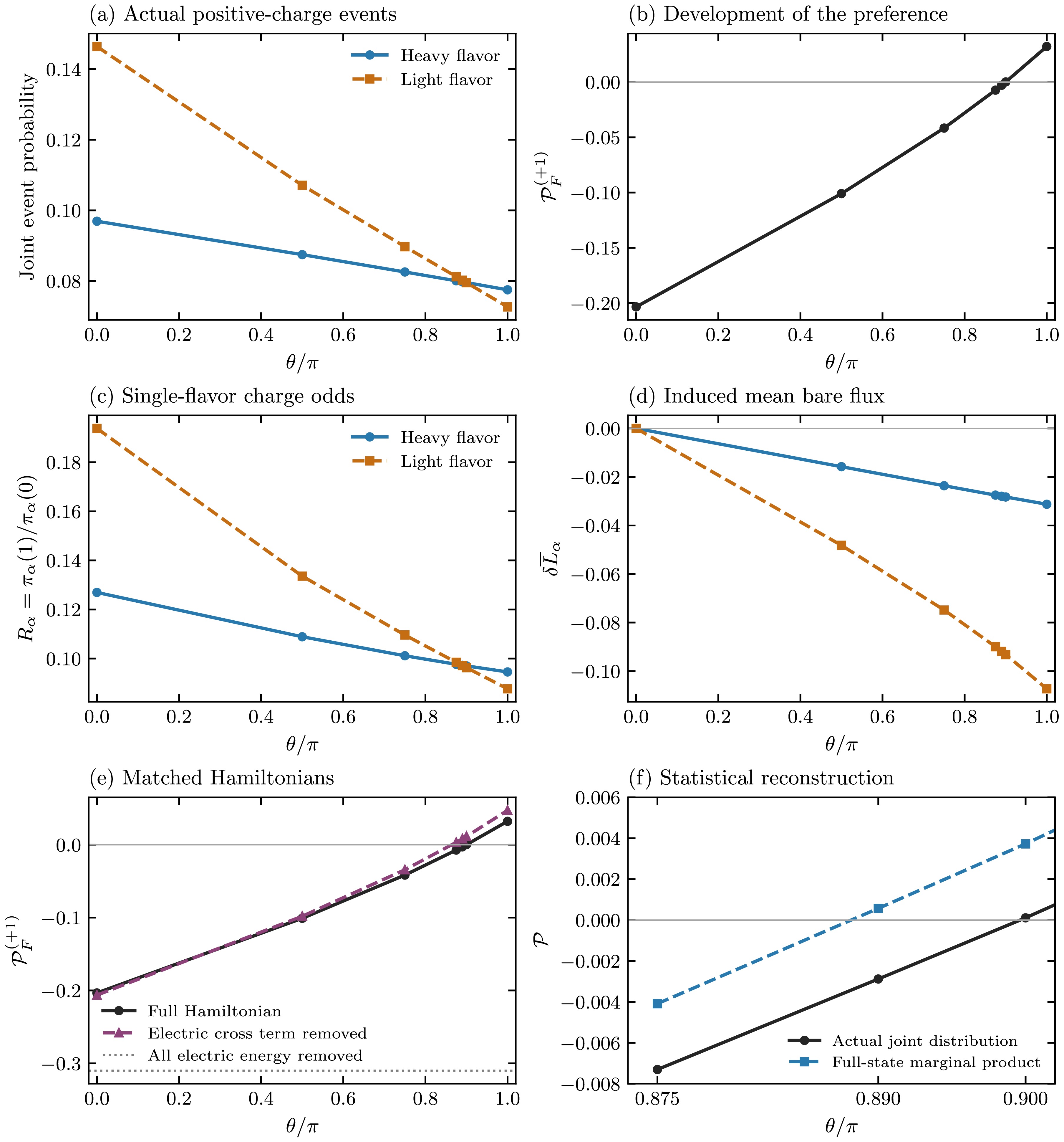
Figure 5. (color online) Mechanism of the intracell heavy-flavor preference at
$ \theta=\pi $ for$ x=4,N_s=16,r=2,m_{\rm{geom}}/g=0.5,h=1 $ and cut$ \ell=7 $ . (a) Actual probabilities of positive-charge events. (b) Corresponding signed polarization, with the negative small-hopping reference at$ \theta=\pi $ noted separately in the text. (c) Single-flavor positive-to-neutral odds. (d) Induced mean bare flux contributions, averaged over the internal links. (e) Matched Hamiltonians: full, with the electric cross term removed, and with all electric energy removed; the lattice masses are unchanged. (f) Actual joint polarization compared with the product of the full state's marginals near the crossing, representing a statistical reconstruction rather than another Hamiltonian. All axes are dimensionless; multiplying a bare flux contribution by g gives its physical electric-field contribution. Symbols denote measured states, and lines serve as guides between sampled angles.$ 0.89<\theta_*/\pi<0.90. $
(41) Component precision is reported in Appendix E.4.
The response is not restricted to the combination for which the sign changes. Figure 6 compares all four charge–cut compositions: the background enhances the light-flavor preference in negative-charge events and shifts positive-charge events toward the heavy flavor in both cut classes. All four polarizations increase across the seven sampled angles. The shift for the positive-charge unit-boundary band is larger than the intra-cell shift, but it does not overcome the stronger initial light-flavor bias. Only the intra-cell positive-charge band crosses the equal-composition point. The non-neutral weight hierarchy remains unchanged, although the weights themselves respond strongly to the background.
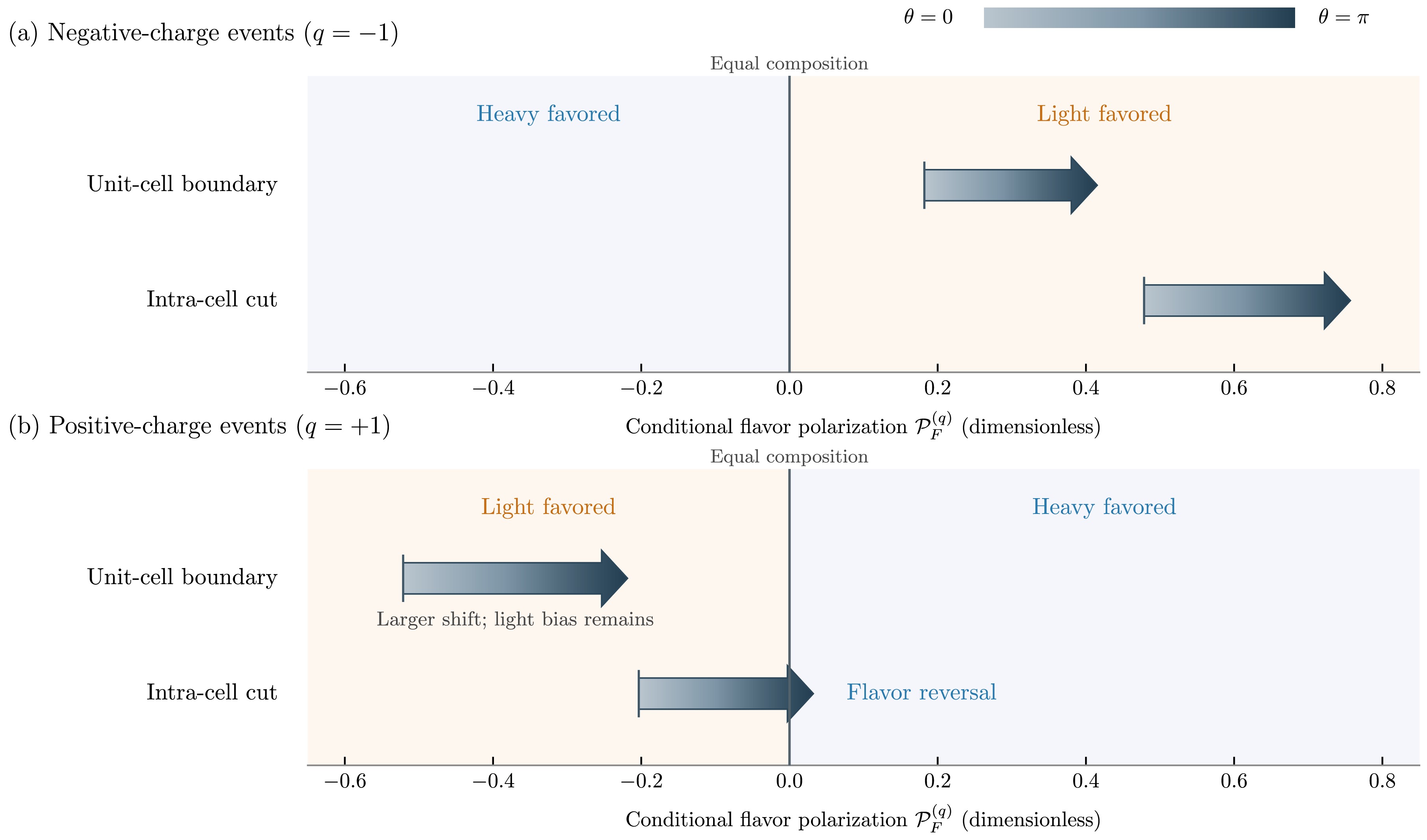
Figure 6. (color online) Four charge–cut responses are shown for the representative parameters of Fig. 5, with unit-cell cut
$ \ell=8 $ and intra-cell cut$ \ell=7 $ . Each quantitative band extends from$ {\cal{P}}_F^{(q)}(0) $ to$ {\cal{P}}_F^{(q)}(\pi) $ on a common dimensionless scale. Its length indicates the field-induced change; its thickness does not encode probability. Shading represents the seven sampled angles using piecewise-linear interpolation. The zero line indicates equal probability for the$ F_A=\pm1 $ components. Positive polarization indicates a light-flavor preference for negative charge but a heavy-flavor preference for positive charge. The larger positive charge shift at the unit-cell boundary still leaves a light-flavor bias, whereas the intra-cell shift reverses this bias. -
The flavor marginals and their positive-to-neutral odds are as follows:
$ \pi_\alpha(k;\theta)=\Pr(Q_{\alpha,A}=k;\theta),\qquad R_\alpha(\theta)=\frac{\pi_\alpha(1;\theta)}{\pi_\alpha(0;\theta)}. $
(42) They include all charges of the other flavor. The light-to-heavy odds ratio
$ R_2/R_1 $ decreases from approximately$ 1.53 $ to$ 0.93 $ , crossing unity [Fig. 5(c)].The corresponding charge rearrangement is independently measured through
$ L_{\alpha,n}=\sum\limits_{k=0}^n\left[n_{k,\alpha}-\frac{1-(-1)^k}{2}\right], \; \overline L_\alpha=\frac{1}{N_s-1}\sum\limits_{n=0}^{N_s-2}\langle L_{\alpha,n}\rangle . $
(43) Both flavors contribute to a single physical field,
$ E_n/g=L_{1,n}+L_{2,n}+b $ . As the background changes from zero to π, the induced mean shifts are$ \delta\overline L_1\simeq-0.031 $ and$ \delta\overline L_2\simeq-0.107 $ [Fig. 5(d)]. This larger opposing response of the light flavor is consistent with the unequal event suppression measured above. The joint probabilities establish the reversal; the average flux response alone does not determine the conditional flavor composition.The matched Hamiltonians separate the external source from the quadratic electric energy. Removing all of
$ H_E $ also removes the source and leaves the light flavor favored in the free chain,$ {\cal{P}}_F^{(+1)}\simeq-0.310 $ . To retain the same source while removing only the quadratic flux term, we use$ \begin{aligned}[b] H_{\rm{src}} =\;&H-K\sum\limits_{n=0}^{N_s-2}L_n^2\\ =\;&H_{\rm{mass}}+H_{\rm{hop}}+2Kb\sum\limits_{n=0}^{N_s-2}L_n+(N_s-1)Kb^2\mathbf1. \end{aligned} $
(44) The masses, hopping parameters, geometry, and canonical particle numbers remain fixed. This noninteracting control already favors the heavy flavor at
$ \theta=\pi/2 $ , with$ {\cal{P}}_F^{(+1)}\simeq0.064 $ and$ W_F^{(+1)}\simeq0.156 $ ; thus, composition reversal does not require the quadratic electric interaction. At$ \theta=\pi $ , however, the system reverts to a preference for the light flavor, and the positive-charge event becomes rare (Table 2); Appendix E.6 shows the full curve.Electric terms retained $ p_+ $ $ p_- $ $ W_F^{(+1)} $ $ {\cal{P}}_F^{(+1)} $ None $ 0.102963 $ $ 0.195546 $ $ 0.298509 $ $ -0.310153 $ Source only $ 2.180\times10^{-6} $ $ 3.973\times10^{-6} $ $ 6.153\times10^{-6} $ $ -0.291327 $ Self-energies and source $ 0.071605 $ $ 0.065147 $ $ 0.136752 $ $ 0.047223 $ Full electric energy $ 0.077496 $ $ 0.072666 $ $ 0.150162 $ $ 0.032165 $ Table 2. Matched electric-term control results at
$ \theta=\pi $ ,$ x=4,N_s=16,r=2,h=1 $ , with$ m_{\rm{geom}}/g=0.5 $ and intra-cell cutoff$ \ell=7 $ . The masses and canonical particle numbers are unchanged. Here,$ p_+=p_{+1,+1} $ and$ p_-=p_{+1,-1} $ denote heavy- and light-flavor positive-charge events, respectively. All entries are dimensionless. Removing all electric energy also removes the source, making the corresponding row independent of θ.Restoring the individual electric self-energies, while excluding the direct interflavor term, gives
$ H_{\rm{dec}}=H-2K\sum\limits_{n=0}^{N_s-2}L_{1,n}L_{2,n}. $
(45) This control retains each flavor's electric self-energy, its coupling to the common background, and the original two-flavor lattice mass shift. Its polarization changes from negative at
$ \theta=0 $ to positive at$ \theta=\pi $ [Fig. 5(e)]. At$ \theta=\pi $ , restoring the self-energies changes$ \langle Q_A\rangle $ from approximately$ -1.88 $ to$ +0.112 $ and restores a positive endpoint with appreciable event weight (Table 2). The quadratic energy penalizes large cumulative flux and restricts charge separation. Restoring the cross term delays the observed crossing and reduces the positive endpoint by approximately$ 32$ %; at zero background, however, the full-model polarization is slightly higher. In the full model at$ \theta=\pi $ , this pair accounts for approximately$ 83$ % of all non-neutral events at the displayed intra-cell cut, with heavy and light shares of approximately$ 51.6$ % and$ 48.4$ % within the pair.Separately, the marginal product of the full interacting state gives
$\begin{aligned}[b]& p_{+1,+1}^{\rm{ind}}=\pi_1(1)\pi_2(0),\qquad p_{+1,-1}^{\rm{ind}}=\pi_1(0)\pi_2(1),\\& {\cal{P}}_{\rm{ind}}=\frac{R_1-R_2}{R_1+R_2}.\end{aligned} $
(46) This is a statistical reconstruction rather than a Hamiltonian deletion. At
$ \theta/\pi=0.89 $ , it is already positive, whereas the actual joint polarization remains negative [Fig. 5(f)]. Thus, joint correlations affect the sign near reversal, even though the individual flavor responses establish the trend. -
The two targeted background probes retain the same unequal-suppression mechanism. Increasing
$ N_s $ from 16 to 20 at fixed$ x=4,r=2 $ shifts the measured bracket to$ (0.82,0.84) $ ; decreasing the mass ratio to$ r=1.5 $ at$ N_s=16 $ yields$ (0.89,0.90) $ , which does not resolve a mass-ratio-induced shift. In both cases, the opposing light-flavor flux response is stronger, and the marginal products become positive before the joint probabilities do. Appendix E.5 gives their probabilities, fluxes, and precision.The small-hopping path provides the complementary local reference. The directed costs are given in Appendix C. Their bias points toward screening, but their squared inverse denominators retain a light-flavor preference for the intra-cell positive-charge pair. The controlled limit and the measured hopping reversal in Appendix C therefore connect the
$ \theta=\pi $ result to its atomic reference; the nonperturbative charge response and Hamiltonian comparisons above explain how the initial preference is overcome. -
The block weights
$ p_{q,f} $ are the joint probability distribution of subsystem gauge charge and flavor imbalance for the chosen matter-site bipartition. Marginalizing over f gives the gauge-charge organization$ p_{Q_A}(q) $ , whereas conditioning on fixed q gives$ p_{F_A\mid Q_A}(f\mid q) $ . The two$ Q_A=\pm1,F_A=\pm1 $ pairs show that the cut geometry reorganizes this distribution rather than merely suppressing one preselected sector:$ Q_A=-1 $ dominates at unit boundaries, whereas$ Q_A=+1 $ dominates for intra-cell cuts. For either$ q=\pm1 $ ,$ W_F^{(q)} $ is the absolute joint weight of the$ F_A=\pm1 $ pair, while$ {\cal{P}}_F^{(q)} $ is the normalized contrast between the two conditional flavor probabilities. Their distinct cut dependence remains important: a small pair weight does not imply weak conditional sensitivity, and a large pair weight does not make the pair maximally polarized.At
$ \theta=\pi $ , the event probabilities show that differential suppression overcomes the initial light-flavor advantage in intra-cell positive-charge fluctuations. The larger opposing light-flavor flux response supports the screening interpretation, but it does not independently determine this conditional preference. The negative-charge compositions simultaneously shift toward the light flavor. The retained source alone can produce composition reversal at intermediate angles, but it yields a light-flavor endpoint with very small positive-charge weight at$ \theta=\pi $ . Electric self-energies restrict the large charge separation and recover a positive-charge endpoint with appreciable event weight in the matched control; the direct interflavor coupling then delays the crossing and reduces the positive polarization. Products of the full state's marginals provide a different statistical comparison: their near-crossing signs show why joint correlations remain relevant.The cut class organizes multiple layers of the reduced state. It determines which non-neutral gauge pair carries most of the probability and competes globally, while mass imbalance redistributes probability both between charge sectors and between flavors within a pair. The cut-dependent initial preferences determine whether the common background-driven shift is sufficient to reverse the flavor composition. Consequently, an unresolved global entanglement gap cannot distinguish a change in gauge-sector identity from a change in fixed-sector probabilities.
The sector weight changes along the fixed geometric-mean scan are the response along the specified mass path, not a pure flavor-breaking susceptibility. The matched equal-mass references show that the common mass increase accounts for most of the intra-cell non-neutral decrease in the matched cases, while the mass-difference term redistributes probability between the complementary charge pairs. A common mass alone does not generate flavor-odd polarization. The matched comparisons and their finite-difference decomposition are given in Appendix E.2.
The atomic reference analysis identifies the lowest nonzero sector-selection processes; quantitative probabilities are determined from the MPS results. The conclusions refer to the finite open-chain, Gauss-law-eliminated matter-site bipartition studied here. The angle and hopping zeros are crossovers, not thermodynamic transitions, and the phase classification of the
$ \theta=\pi $ mass path is not assigned to the entire angle trajectory. The electric-term deletion controls establish sufficiency at the representative parameters; the length and mass-ratio extensions test the charge-response mechanism without repeating those deletion experiments. -
In the two-flavor Schwinger model at
$ \theta=\pi $ , we find that intra-cell positive charge fluctuations can favor the heavier flavor, even though the controlled small-hopping reference favors the lighter flavor. In the representative chain, increasing the background from zero to π suppresses the heavy- and light-flavor event probabilities by$ 20.05$ % and$ 50.37$ %, respectively. Thus, the stronger suppression of the light-flavor contribution overturns its initial advantage. The source alone can already reverse the composition at intermediate angles. At$ \theta=\pi $ , electric self-energies restrict charge separation and restore an appreciable positive charge pair weight with a slight heavy-flavor preference, while direct interflavor coupling weakens this preference and delays the crossing.The background response extends beyond the composition that changes sign. Negative charge events become more strongly dominated by the light flavor, whereas positive charge events shift toward the heavy flavor in both cut classes. The positive charge response at the unit cell boundary is larger, but it does not overcome its stronger initial light-flavor bias; the intra-cell response does. The unequal suppression and flavor reversal are also reproduced in the longer chain and at smaller mass imbalance.
At fixed
$ \theta=\pi $ , changing the staggered cut exchanges the dominant non-neutral gauge sector: the$ Q_A=-1 $ pair dominates at unit cell boundaries, whereas the$ Q_A=+1 $ pair dominates at intra-cell cuts. Mass and geometry comparisons distinguish this sector reordering from changes in pair weight and conditional flavor polarization, while matched mass references separate common-mass and mass-difference contributions. Thus, symmetry resolution distinguishes gauge sector ordering from flavor composition and reveals why a lower bare excitation cost need not determine the flavor composition of a charged vacuum fluctuation. -
The electric energy of the eliminated gauge field contains squares of cumulative charges. For the internal-link convention, let
$\kappa=g^2a/2$ ,$b_\theta=L_{-1}+\theta/(2\pi)$ , and$\delta_R=0$ . Define$ \left(b_\theta+\sum\limits_{k\le n}Q_k\right)^2 = b_\theta^2 +2b_\theta\sum\limits_{k\le n}Q_k +\sum\limits_{k\le n}Q_k^2 +2\sum\limits_{i<j\le n}Q_iQ_j.$
(A1) After summing this expression over the internal links, we define
$ R=N_s-1+\delta_R, \qquad w_i=\max(R-i,0). $
(A2) Then
$ H_E=E_{\mathrm{const}}+\sum\limits_i A_iQ_i+\sum\limits_i B_iQ_i^2+\sum\limits_{i<j}V_{ij}Q_iQ_j, $
(A3) with
$\begin{aligned}[b]& E_{\mathrm{const}}=\kappa R b_\theta^2, \quad A_i=2\kappa b_\theta w_i, \quad B_i=\kappa w_i, \\& V_{ij}=2\kappa\max[R-\max(i,j),0].\end{aligned} $
(A4) When
$\delta_R=0$ ,$w_{N_s-1}=0$ ; thus, the charge on the rightmost matter site does not contribute to the internal-link electric energy. The exact three-state electric MPO uses$ W_i= \left( {\begin{array}{*{20}{c}} {\bf{1}}&{{Q_i}}&{{e_i}}\\ 0&{\bf{1}}&{{V_i}{Q_i}}\\ 0&0&{\bf{1}} \end{array}} \right), $
(A5) where
$i=0,\ldots,N_s-1$ ,$V_i=2\kappa w_i$ , and$e_i=A_iQ_i+B_iQ_i^2$ . For the displayed upper-triangular orientation, the boundary vectors are$ v_L=(1,0,0), \qquad v_R=(0,0,1)^{\mathsf T}. $
(A6) The operator-independent contribution
$E_{\mathrm{const}} {\bf{1}}$ is included once in$e_0$ , consistent with the MPO construction, rather than being represented by a second identity MPO. This yields bond dimension 3, independent of$N_s$ . Including the hopping and mass terms gives a full-Hamiltonian bond dimension of 7 for the conventions used here. -
For a cut after
$\ell$ physical sites,$ Q_A=N_A-2\lfloor\ell/2\rfloor, \qquad F_A=N_{1,A}-N_{2,A}. $
(A7) The tensor network representation labels each block by
$(N_A,F_A^{\mathrm{backend}})$ , with$ F_A=F_A^{\mathrm{backend}} $ , and the analysis maps this label to the physical$(Q_A,F_A)$ . Sector-blocked ED singular-value decompositions provide the reference mapping. Charges are never assigned to degenerate singular subspaces based on an unresolved SVD. -
The matter sites are located at
$ z_n=(n+\frac{1}{2})a $ between the geometric boundaries$ z=0 $ and$ z=N_sa $ . Therefore,$ L_{\mathrm{phys}}=N_sa $ . The distance between the outermost matter sites,$ (N_s-1)a $ , is a distinct geometric quantity and is not used as the volume label. -
The control tests in this appendix refer to the primary mass grid with
$ \theta=\pi,h=1 $ and the specified centering tests. The exact symmetry maps used for sector validation are given in Appendix D.3; additional interpolation and matched-mass convergence tests are collected in Appendix E. -
We validate the Hamiltonian construction, ground-state calculations, and symmetry-resolved Schmidt spectra against exact diagonalization. For
$ N_s=2,3,4 $ , the MPO agrees with sparse ED at the matrix level, and small-system DMRG reproduces the energies and resolved Schmidt weights. The flavor-exchange symmetry provides an additional consistency check. Table B1 summarizes these benchmarks. Solver details and convergence diagnostics are provided below, and reciprocal checks are reported in Appendix D.Validation Sizes Diagnostic Result MPO versus sparse ED $ N_s=2,3,4 $ maximum matrix-element difference (g) $ 1.78\times10^{-15} $ DMRG versus ED $ N_s=4 $ sector ground-state energy difference (g) $ 1.20\times10^{-14} $ sector DMRG versus sector ED $ N_s=8 $ sector ground-state energy difference (g) $ 4.53\times10^{-12} $ sector DMRG benchmark $ N_s=8 $ energy variance ( $ g^2 $ )total $ 5.21\times10^{-11} $ ; per site$ 6.51\times10^{-12} $ resolved Schmidt spectrum $ N_s=2,3,4 $ ED–MPS block labels and probabilities max probability difference $ 7.62\times10^{-14} $ ; 0 label mismatchesTable B1. Numerical validation hierarchy. The listed errors are either maxima or representative benchmark values for the stated comparisons. Hamiltonian matrix elements and energy differences are reported in units of g, energy variances in units of
$ g^2 $ , and probability differences are dimensionless.The states used in the main analysis satisfy the convergence criteria in Sec. II.E.2. Comparisons between successive bond dimensions show that the
$ q=+1 $ and$ q=-1 $ flavor components, pair weights, and signed polarizations remain stable over the available bond-dimension increases. Detailed componentwise convergence diagnostics are provided in Appendices B.4 and E.1. The minimum unequal-mass$ q=+1 $ numerator-to-drift ratio is$ 5.165\times10^4 $ ; the sign check is performed directly on the numerator and is not inferred from the stability of$ q=-1 $ . -
The cut classification introduced in Sec. II.B.3 has a direct empirical counterpart in these states. Finite-interval calculations for the Schwinger model and open-boundary tensor-network studies can exhibit strong boundary and profile effects [14, 18], and boundary-sensitive symmetry resolution is known more generally [28]. In our data, bond-by-bond entanglement profiles also display a pronounced alternating component associated with the staggered cut class. In the central-neighbor calculations, the spread (maximum minus minimum) across the three cuts reached approximately 0.334 for the entropy and approximately 1.69 for the global entanglement energy gap.
The bond profiles in Fig. B1 show that this alternation extends beyond the central-neighbor controls. Class-resolved centered-cut values confirm the same ordering when either cut class occupies the geometric center (Table B2).
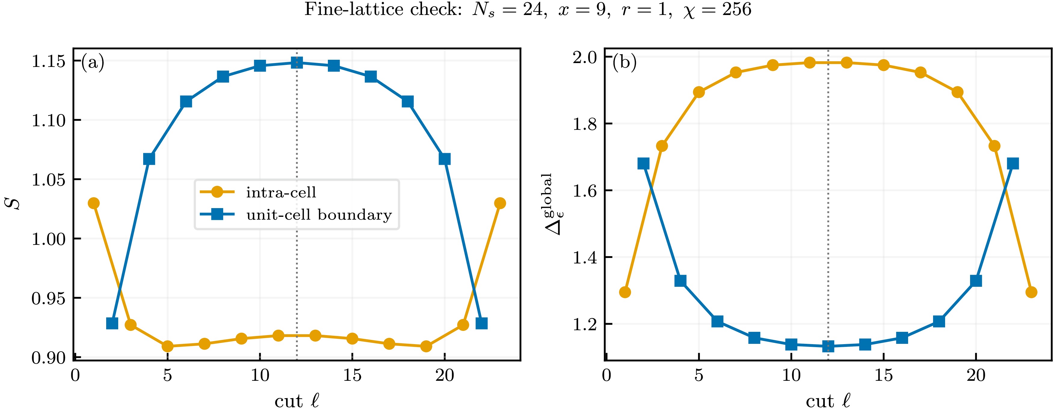
Figure B1. (color online) Bond-resolved (a) entanglement entropy and (b) global entanglement energy gap for the state with
$ N_s=24 $ ,$ x=9 $ ,$ r=1 $ , and$ \chi=256 $ . Intra-cell and unit-cell-boundary cuts are distinguished, and the dotted line marks the central unit-cell boundary at$ \ell=12 $ . Both quantities are dimensionless; the entropy is reported in nats, and$ \ell $ denotes an integer cut index.$N_s$ $r$ $S_{\mathrm{intra}}$ $S_{\mathrm{unit}}$ $\Delta_{\epsilon,\mathrm{intra}}^{\mathrm{global}}$ $\Delta_{\epsilon,\mathrm{unit}}^{\mathrm{global}}$ 18 1 0.733201 1.064565 2.323677 1.230324 18 2 0.745423 1.065650 2.349588 0.748087 24 1 0.738580 1.072955 2.329807 1.213897 24 2 0.770881 1.087687 2.341787 0.647335 Table B2. Cut-class-resolved entropy and global entanglement energy gap for the
$r=1$ and$r=2$ central-neighbor calculations. All rows correspond to$x=4$ and$\chi=256$ . When a class is represented by two symmetry-related neighboring cuts, the mean is reported; the maximum left–right difference across both observables is$3.3\times10^{-10}$ . The entropy is computed using the natural logarithm and is reported in nats; the global gap is a difference between dimensionless entanglement energies and is therefore dimensionless.The class-resolved central-neighbor values in Table B2 show that unit-cell boundaries have higher entropy and a smaller global gap, regardless of whether the cut class occurs at the geometric center or at its two neighboring positions.
Figure B2 shows the absolute joint-probability composition underlying the reference-subtracted response in Fig. 3.
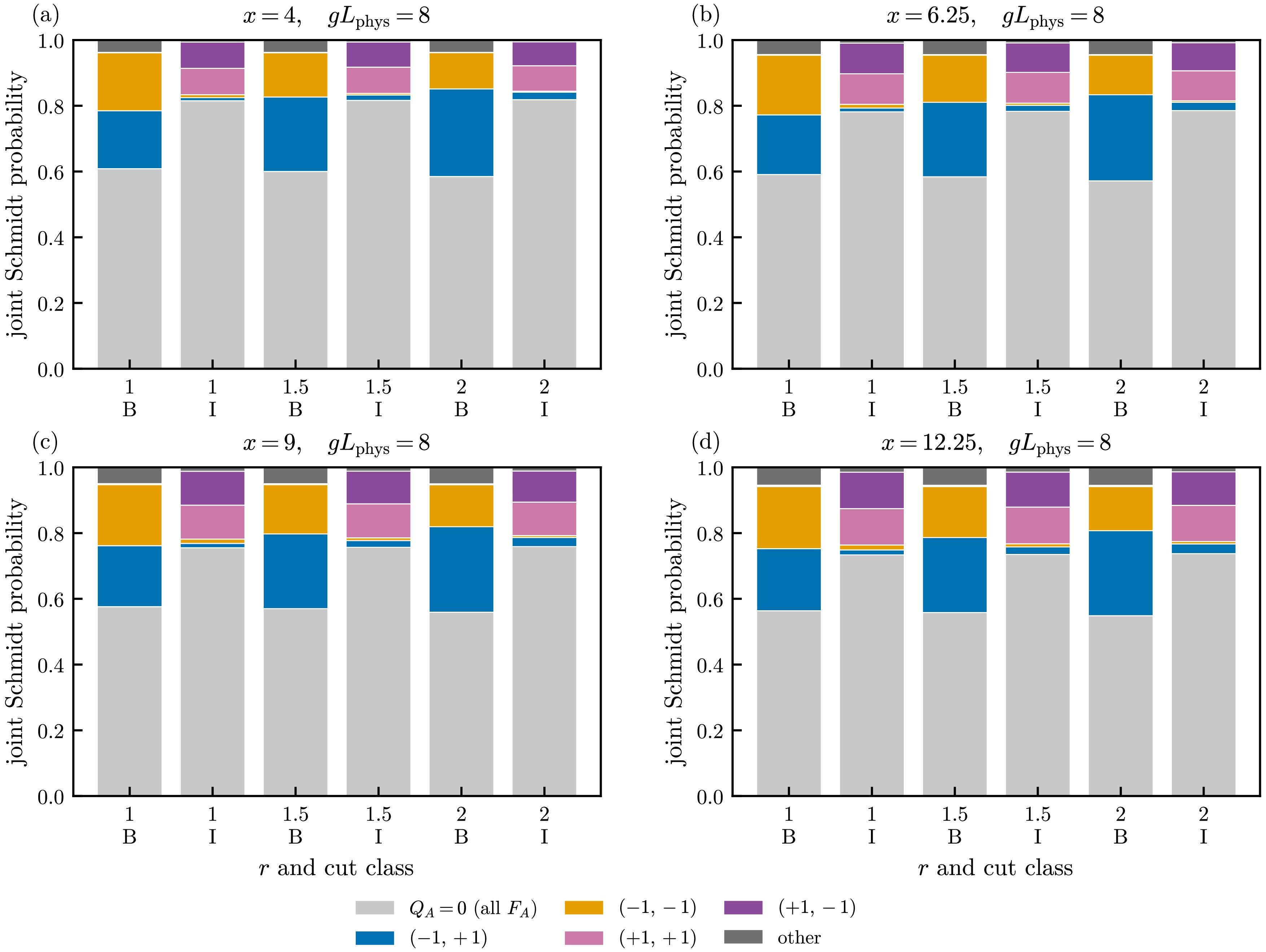
Figure B2. (color online) Absolute composition of the major blocks in the joint Schmidt probability distribution at
$ gL_{\mathrm{phys}}=8 $ for$ r=1,1.5,2 $ . Each mass ratio is shown for the selected unit-cell boundary (B) and the mirror-combined intra-cell cut class (I) across all four sampled spacings. The six categories comprise all$ Q_A=0 $ blocks, the two$ Q_A=-1,F_A=\pm1 $ partner blocks, the two$ Q_A=+1,F_A=\pm1 $ partner blocks, and all remaining sectors. Each bar sums to unity using the complete Schmidt spectrum. All probabilities and the parameters x, r, and$ gL_{\mathrm{phys}} $ are dimensionless. -
A basis state is represented by a
$ 2N_s $ -mode occupation bit string in the site-major ordering described in Sec. II.B. Fermionic operations and Jordan–Wigner signs are applied directly to the bit strings, and full or symmetry-restricted Hamiltonians are assembled as complex sparse matrices. In the MPS representation, local fermion operators carry the corresponding metadata, ensuring that inter-site parity strings are inserted consistently; small-system matrix reconstruction tests verify the resulting signs.Matrix-level validation compares the hopping, mass, electric, and full MPOs against ED at
$ N_s=2,3,4 $ . DMRG energies, term energies, local charges, electric-flux moments, Schmidt probabilities, and subsystem labels are compared with ED for small systems. A dominant-block assignment is marked ambiguous when the difference between the two largest block weights is below$ 10^{-6} $ ; no point in the main analysis is ambiguous. The unrestricted ED basis follows the site-major bit-string order, and symmetry-restricted bases retain explicit forward and inverse maps. Dense Hermitian diagonalization is used when the matrix dimension is at most 16 or when the requested eigenpairs span the matrix. If sparse diagonalization does not return the requested eigenpairs, dense Hermitian diagonalization is used for matrices of dimension at most 256. Solver residuals are monitored in all validation calculations. -
Finite-system DMRG [38, 41] employs deterministic initialization, increasing bond dimensions, and warm starts between successive values of χ. We define the energy variance per site as
$ v_E=\frac{\langle H^2\rangle-\langle H\rangle^2}{N_s}. $
(B1) For the main quantitative analysis,
$v_E$ and the maximum discarded weight must be less than$10^{-6}$ , and the changes between the two largest available bond dimensions must satisfy$ |\Delta E|<10^{-6},\qquad \max\limits_{k\le20}|\Delta\epsilon_k|<10^{-3},\qquad \Delta O_{\mathrm{bulk}}<10^{-3}. $
(B2) The auxiliary bulk-window observables define the convergence monitor
$ \Delta O_{\mathrm{bulk}} $ . Their deterministic construction and the complete definitions of$ L_{\mathrm{bulk}} $ ,$ C_\pm^{\mathrm{bulk}} $ , and$ \Delta O_{\mathrm{bulk}} $ are given below. The mechanism analysis also measures the flavor-resolved charge marginals and the induced flux averaged over all internal links, as defined in Sec. III.C.2.Here,
$ \Delta E $ is the change in the canonical-sector ground-state energy between the two largest available bond dimensions. Entanglement levels are matched by$ (Q_A,F_A) $ and block rank before the largest drift among the first 20 matched levels is computed. State normalization, the canonical sector, Hamiltonian parameters, and the cut definition are verified independently of the numerical thresholds. Reaching the prescribed maximum bond dimension is not, by itself, taken as evidence of convergence; convergence is assessed using the energy, spectrum, local-observable, and discarded-weight criteria stated above and reported in Appendix B.The default comparison uses
$ \chi=128,256 $ , and two matched triplets with$ r=1,1.5,2 $ were extended to$ \chi=384 $ . At$ x=12.25,N_s=40 $ , the$ \chi=128 $ to 256 total-energy drifts are$ 1.15 $ –$ 1.44\times10^{-6} $ ; at$ x=12.25,N_s=36 $ , the equal-mass reference has a drift of$ 1.080\times10^{-6} $ . These cases are evaluated at$ \chi=384 $ , where they satisfy the stated criteria. A reference-subtracted response is retained only when both the unequal-mass state and its matched reference pass the convergence tests; the remaining matched sets pass at$ \chi=256 $ .For the 32 unequal-mass states, Table E1 summarizes direct componentwise changes between the two largest available bond dimensions for both charges and cut classes. The mirror-related intra-cell probabilities are combined before the polarization is formed and differenced. The finite-MPS states were generated with the specified TeNPy truncation controls, including
$ \mathrm{svd\_min}=10^{-12} $ . For the block-weight reconstruction, every Schmidt value present in each available MPS state was summed without the$ 10^{-12} $ probability filter used for the low-lying level tables.Quantity $ q=-1 $ , B$ q=-1 $ , I$ q=+1 $ , B$ q=+1 $ , IMedian Maximum Median Maximum Median Maximum Median Maximum $ p_{q,+1} $ $ 1.25\times10^{-8} $ $ 2.25\times10^{-7} $ $ 1.24\times10^{-8} $ $ 2.36\times10^{-7} $ $ 9.59\times10^{-10} $ $ 1.46\times10^{-8} $ $ 7.44\times10^{-10} $ $ 3.87\times10^{-8} $ $ p_{q,-1} $ $ 6.22\times10^{-9} $ $ 1.40\times10^{-7} $ $ 6.82\times10^{-9} $ $ 1.81\times10^{-7} $ $ 7.79\times10^{-10} $ $ 1.39\times10^{-8} $ $ 1.60\times10^{-9} $ $ 4.00\times10^{-8} $ $ N_F^{(q)} $ $ 3.94\times10^{-9} $ $ 1.58\times10^{-7} $ $ 4.91\times10^{-9} $ $ 1.58\times10^{-7} $ $ 2.61\times10^{-10} $ $ 4.54\times10^{-9} $ $ 1.34\times10^{-9} $ $ 1.62\times10^{-8} $ $ W_F^{(q)} $ $ 1.88\times10^{-8} $ $ 3.26\times10^{-7} $ $ 1.87\times10^{-8} $ $ 4.04\times10^{-7} $ $ 1.70\times10^{-9} $ $ 2.76\times10^{-8} $ $ 2.44\times10^{-9} $ $ 7.85\times10^{-8} $ $ {\cal{P}}_F^{(q)} $ $ 3.53\times10^{-9} $ $ 1.34\times10^{-7} $ $ 2.00\times10^{-7} $ $ 2.87\times10^{-6} $ $ 2.39\times10^{-7} $ $ 1.93\times10^{-6} $ $ 7.75\times10^{-9} $ $ 9.45\times10^{-8} $ Table E1. Absolute changes computed directly between the two largest available bond dimensions for 32 unequal-mass primary states. B denotes the selected unit-cell boundary; I uses mirror-combined intra-cell probabilities before computing the polarization. Each column pair reports the median and maximum change. All quantities are dimensionless;
$ N_F^{(q)}=p_{q,+1}-p_{q,-1} $ determines the sign. These values are stability diagnostics, not rigorous error bounds.For
$ M=N_s-1 $ internal links, the default bulk window is the half-open interval$ [j_0,j_1) $ . Define$ \begin{array}{l} w_0 =\max \left[2,\text{round}_{\mathrm{ties\rm-to\rm-even}} \left(\dfrac{M}{2}\right)\right],\\ \widetilde w =\left\{ {\begin{array}{*{20}{l}} {{w_0},}&{{w_0}\,\text{mod} \,2 = M\,\text{mod} \,2,}\\ {{w_0} + 1,}&{{\rm{otherwise}},} \end{array}} \right.\\ w =\min(M,\widetilde w),\qquad j_0=(M-w)/2,\qquad j_1=j_0+w. \end{array} $
(B3) The cap includes the small validation systems; for
$ N_s=2 $ , it gives$ M=1 $ and$ [j_0,j_1)=[0,1) $ . Let$ [s_0,s_1) $ denote the deterministic central 50% site window obtained using the same rounding, parity-matching, and profile-length cap prescription, with the site-profile length$ N_s $ replacing the internal link length M. The two monitored bare staggered-occupation diagnostics are$ C_{\pm}^{\mathrm{bulk}} = \frac{1}{s_1-s_0} \sum\limits_{n=s_0}^{s_1-1} (-1)^n \left( \langle n_{n,1}\rangle \pm \langle n_{n,2}\rangle \right). $
(B4) where
$ C_+^{\mathrm{bulk}} $ and$ C_-^{\mathrm{bulk}} $ are referred to as the condensate sum and condensate difference, respectively. No additional staggered-background subtraction or continuum renormalization is applied to these convergence diagnostics. Here,$ L_{\mathrm{bulk}} $ denotes the arithmetic mean of the bare link flux over the central deterministic internal-link window. With$ \Delta $ denoting the change between the two largest available bond dimensions, we define$ \Delta O_{\mathrm{bulk}} = \max \left( |\Delta L_{\mathrm{bulk}}|, |\Delta C_+^{\mathrm{bulk}}|, |\Delta C_-^{\mathrm{bulk}}| \right). $
(B5) For a fractional interval
$ [f_0,f_1] $ , the corresponding integer window is$ [\lceil f_0M\rceil,\lceil f_1M\rceil) $ . The alternatives$ [0.35,0.65] $ and$ [0.40,0.60] $ are used only for bulk-profile calculations with$ N_s\ge16 $ . In contrast, small-system ED–MPS validation compares link-resolved moments directly. These bulk-window flux and condensate diagnostics are used to check convergence and boundary sensitivity. The flavor-resolved flux response in Sec. III.C.2 is a distinct physical observable averaged over all internal links.Two
$ x=12.25 $ systems include a three-point$ \chi=128,256,384 $ ladder for both the equal-mass reference and$ r=2 $ . Table B3 reports the successive absolute changes in$ D_F $ at$ r=2 $ .system $ |D_{F,256}-D_{F,128}| $ $ |D_{F,384}-D_{F,256}| $ $ gL_{\rm{phys}}=10.29 $ ,$ N_s=36 $ $ 4.47\times10^{-7} $ $ 1.07\times10^{-9} $ $ gL_{\rm{phys}}=11.43 $ ,$ N_s=40 $ $ 8.57\times10^{-7} $ $ 1.78\times10^{-9} $ Table B3. Three-point bond-dimension convergence sequences for
$ D_F $ at$ r=2 $ . The observable and its successive differences are dimensionless;$ gL_{\mathrm{phys}} $ , r, and χ are dimensionless, whereas$ N_s $ denotes the number of sites.Across the 42 primary states, the largest combined probability mass of the two target blocks below the low-level tabulation threshold
$ \lambda=10^{-12} $ is$ 9.97\times10^{-12} $ , corresponding to at most$ 3.15\times10^{-10} $ of their combined weight. These tail levels are included in the reported$ p_\pm $ . -
For the natural cell
$(2j,2j+1)$ , a cut$\ell$ lies between sites$\ell-1$ and$\ell$ . An odd$\ell$ corresponds to an intra-cell even-to-odd cut, whereas an even$\ell$ corresponds to an odd-to-even unit-cell-boundary cut. Consequently, the central cut is a unit-cell boundary for$N_s\text{mod}4=0$ and an intra-cell cut for$N_s\text{mod}4=2$ . The primary mass-grid comparison selects the unit-cell boundary that minimizes$|\ell-N_s/2|$ , together with its adjacent intra-cell cuts. If the two sides are equidistant, the left boundary (the smaller$\ell$ ) is selected deterministically; the reflection-related partner is retained as a consistency check.The existing
$ N_s=18,x=4 $ states exhibit the reverse centering pattern relative to the main$ N_s\text{mod}4=0 $ grid: cut$ \ell=9 $ is a precisely centered intra-cell cut, and$ \ell=8,10 $ are the adjacent unit-cell boundaries. Table B4 reports the complete-Schmidt probabilities. At$ r=2 $ , the centered intra-cell cut still has a much smaller$ W_F^{(-1)} $ and a larger$ {\cal{P}}_F^{(-1)} $ than either adjacent unit-cell boundary. The mean of the two$ N_s=18 $ unit-cell boundaries also lies between the central unit-cell-boundary values at$ N_s=16 $ and 20 for$ p_\pm $ ,$ W_F^{(-1)} $ , and$ {\cal{P}}_F^{(-1)} $ . This comparison isolates cut class from the one-site centering offset.r cut class $ p_{-1,+1} $ $ p_{-1,-1} $ $ W_F^{(-1)} $ $ {\cal{P}}_F^{(-1)} $ 1 central intra-cell $ 0.00967440 $ $ 0.00967440 $ $ 0.0193488 $ $ -3.25\times10^{-11} $ 1 adjacent unit mean $ 0.17737415 $ $ 0.17737415 $ $ 0.3547483 $ $ 3.95\times10^{-12} $ 2 central intra-cell $ 0.02640104 $ $ 0.00312267 $ $ 0.0295237 $ $ 0.788464 $ 2 adjacent unit mean $ 0.27435205 $ $ 0.10861952 $ $ 0.3829716 $ $ 0.432754 $ Table B4. Reversed-centering control for
$ x=4 $ ,$ N_s=18 $ , and$ \chi=256 $ , evaluated using complete Schmidt spectra. The geometric center is the intracell cut$ \ell=9 $ ; unit-boundary entries are computed as the mean of the values at$ \ell=8 $ and$ \ell=10 $ , for which the maximum difference in the displayed quantities is$ 3.8\times10^{-11} $ . All probabilities and polarizations are dimensionless.Complete-spectrum reconstruction and successive-χ comparisons show that
$ W_F^{(\pm1)} $ and$ {\cal{P}}_F^{(\pm1)} $ remain stable over the available bond dimensions, while reflection-related intra-cell cuts agree to numerical precision.For fixed x, r, and cut class, the available data comprise two or three lengths rather than a uniform Cartesian grid. Across all 24 such sequences,
$ W_F^{(-1)} $ is nondecreasing, whereas$ W_F^{(+1)} $ decreases. For every unequal-mass sequence, the signed values of both conditional polarizations are nondecreasing along the available lengths. Because$ {\cal{P}}_F^{(+1)} $ is negative at unit-cell boundaries, however, this statement does not imply a common trend in its magnitude across cut classes. These results reflect finite-length sensitivities rather than length-scaling laws; in particular, the total non-neutral probability is not strictly monotone in every intra-cell sequence. -
This section summarizes the lowest-order nonzero local processes and the sectors they generate, followed by a controlled small-hopping reference for the flavor preference. The arguments for sector selection are based on the lattice Hamiltonian, whereas the full-hopping probabilities are measured from the MPS.
$\begin{aligned}[b]& H_0=H_{\mathrm{mass}}+H_E, \qquad V=H_{\mathrm{hop}}, \\& t=\frac{1}{2a}, \qquad \mu_\alpha=m_\alpha-\frac{g^2a}{4}>0.\end{aligned} $
(C1) The atomic reference configuration has every even site empty and both flavors present on every odd site. For
$ L_{-1}=0 $ and$ \theta=\pi $ , the shifted field$ L_n+\theta/(2\pi) $ is$ +1/2 $ on every internal link. Moving flavor α from an occupied odd site to its right-hand neighboring empty even site costs$ \Delta_\alpha=2\mu_\alpha=2m_\alpha-\frac{g^2a}{2}. $
(C2) The shifted field on that link changes from
$ +1/2 $ to$ -1/2 $ ; therefore, the elementary dipole incurs no electric energy cost at$ \theta=\pi $ . -
We denote a doubly occupied site by
$ 12 $ , an empty site by 0, and the flavor distinct from α by$ \bar\alpha $ . At an even cut$ \ell $ , the first-order process across the cut is$ |12\, |\,0\rangle \xrightarrow{\;c_{\ell,\alpha}^{\dagger}c_{\ell-1,\alpha}\;} |\bar\alpha\, |\,\alpha\rangle . $
(C3) This process transfers one fermion out of A and therefore yields
$ Q_A=-1 $ . Since$ F_A=N_{1,A}-N_{2,A} $ ,$ \begin{aligned}[b]&\alpha=1:\ (Q_A,F_A)=(-1,-1), \\& \alpha=2:\ (Q_A,F_A)=(-1,+1).\end{aligned} $
(C4) The target sectors first appear after one hop at this cut; their finite-hopping probabilities are measured from the MPS.
At an odd cut, the adjacent atomic occupation is instead
$ \lvert0\mid12\rangle $ . The only allowed first-order cross-cut hop is directed into A,$ |0\, |\,12\rangle \xrightarrow{\;c_{\ell-1,\alpha}^{\dagger}c_{\ell,\alpha}\;} |\alpha\, |\,\bar\alpha\rangle, $
(C5) and produces
$ Q_A=+1 $ . Its shifted cut field changes from$ +1/2 $ to$ +3/2 $ , yielding the excitation energy$ \Delta_\alpha^{(Q_A=+1)}=2\mu_\alpha+g^2a=2m_\alpha+\frac{g^2a}{2}. $
(C6) Producing
$ Q_A=-1 $ requires reverse transfer from A to$ \bar A $ , which is blocked by an empty source and an occupied destination. A single preparatory hop cannot remove both obstructions; an initial hop in the allowed direction instead yields$ Q_A=+1 $ , from which one additional hop can at most return the system to$ Q_A=0 $ . Preparing a particle and a vacancy of the same flavor on opposite sides and then transferring it across the cut reaches$ Q_A=-1 $ in three hops, using the labels of Eq. (C4). The leading amplitude is therefore third order, whereas the complementary$ Q_A=+1 $ sector is accessible at first order.No quantitative conclusions about the full Schmidt sector weights follow from these orders at the primary
$ h=1 $ parameters. In particular,$ t/\Delta_2\simeq2.19 $ –$ 3.10 $ at representative$ r=2 $ points, so the hopping expansion is not controlled. Each sector probability sums over all Schmidt values and all left–right configurations, including connected dressing, path interference, normalization, and higher-order processes. The order count identifies sector accessibility, whereas the controlled small-hopping calculation below provides the limiting flavor preference. -
At
$ \tau=\theta/\pi $ , the directed single-hop costs are$\begin{aligned}[b]& \Delta_\alpha^\rightarrow =2m_{{\rm{lat}},\alpha}+K(1-\tau)=2m_\alpha-K\tau,\\& \Delta_\alpha^\leftarrow=2m_{{\rm{lat}},\alpha}+K(1+\tau)=2m_\alpha+K\tau. \end{aligned}$
(C7) We denote by
$ \Delta_\alpha^+=\Delta_\alpha^{(Q_A=+1)} $ the leftward excitation energy in Eq. (C6) and multiply the hopping term by a dimensionless parameter h, while holding the diagonal Hamiltonian fixed.For the intra-cell
$ q=+1 $ pair, first-order wave-function perturbation theory gives$ \begin{aligned}[b]& p_{+1,+1}(h) =A_+h^2+O(h^4), A_+ =\frac{t^2}{(\Delta_1^+)^2},\\& p_{+1,-1}(h) =A_-h^2+O(h^4), A_- =\frac{t^2}{(\Delta_2^+)^2}, \end{aligned} $
(C8) These coefficients are dimensionless. Odd powers of the hopping amplitude do not contribute to these probabilities: a sign change of all nearest-neighbor hopping amplitudes can be implemented by an on-site staggered phase rotation, which leaves the charge projectors invariant. The limiting intracell polarization is
$ {\cal{P}}_{\rm{LO}} =\lim\limits_{h\to0^+}{\cal{P}}_{F, {\rm{intra}}}^{(+1)} =\frac{(\Delta_2^+)^2-(\Delta_1^+)^2}{(\Delta_2^+)^2+(\Delta_1^+)^2}. $
(C9) It is not assigned to the zero-weight point at
$ h=0 $ .At
$ x=4, r=2, m_{\rm{geom}}/g=0.5 $ ,$ \begin{array}{l} \Delta_1^+/g =1.66421356, \ \ \ \Delta_2^+/g =0.95710678,\\ \ \ \ A_+ =0.36106209, \ \ \ A_- =1.09163943,\\ \ \ \ {\cal{P}}_{\rm{LO}} =-0.50290947. \end{array} $
(C10) At
$ x=9, r=2 $ , the corresponding limit is$ -0.53198955 $ , and at$ x=4, r=1.5 $ , it is$ -0.31321481 $ . The values for$ h=0.02 $ in these other families are consistent with their respective negative limits. At fixed spacing and mass ratio, changing$ N_s $ does not change these leading local denominators.The local expansion parameters are
$ ht/\Delta_\alpha^{\rightarrow ,\leftarrow} $ , where the arrows denote the two costs in Eq. (C7). At the original hopping strength$ h=1 $ , they are not small: for$ r=2 $ ,$ t/\Delta_2^\rightarrow $ ranges from$ 2.19 $ to$ 3.10 $ as x varies from$ 4 $ to$ 12.25 $ , while$ t/\Delta_2^\leftarrow $ ranges from$ 1.04 $ to$ 2.06 $ . The latter quantity is the denominator ratio for the target intra-cell process. The small-hopping expansion provides a controlled reference near$ h=0 $ ; the finite-hopping reversal is established by the nonperturbative calculations. These local ratios do not determine the convergence radius of the full series, and the polarization zero$ h_* $ is not a perturbative-breakdown threshold. -
The small-h states enable a local numerical comparison beyond Eq. (C8):
$ {\cal{P}}(h)={\cal{P}}_{\rm{LO}}+c_2h^2+O(h^4),\qquad c_2\simeq6.21. $
(C11) To resolve its component origin, write
$ p_{+1,\pm1}(h)=A_\pm h^2\bigl[1+b_\pm h^2+O(h^4)\bigr].$
(C12) Expanding the ratio, rather than only its numerator, gives
$ c_2=\frac{1-{\cal{P}}_{\rm{LO}}^2}{2}(b_+-b_-). $
(C13) A common normalization correction cancels in
$ b_+-b_- $ . Thus, a positive$ c_2 $ reflects different relative corrections to the two components rather than their common normalization reduction.A fit at small h for
$ x=4,N_s=16,r=2 $ , using$ h=0.005,0.01,0.02 $ , gives$ b_+\simeq-5.92 $ ,$ b_-\simeq-22.55 $ , and$ c_2\simeq6.21>0 $ . Thus, the initially favored$ F_A=-1 $ component undergoes the larger relative reduction. This local expansion is not extrapolated to the reversal region. -
The interpolation used to connect the atomic reference with the original Hamiltonian is
$ H(h)=H_{\rm{mass}}+H_E+hH_{\rm{hop}},\qquad 0\leq h\leq1. $
(C14) This fixes
$ g,a,N_s,m_{{\rm{lat}},\alpha},\theta=\pi,L_{-1} $ , and the canonical sector. For$ h>0 $ , the same operator admits an equivalent standard Hamiltonian representation,$ H(h;g,a,\{m_\alpha\}) =\sqrt h\,H_{\rm{std}} \left(g,\frac{a}{\sqrt h}, \left\{\frac{m_\alpha}{\sqrt h}\right\}\right). $
(C15) The lattice mass shifts transform by the same factor; therefore, the positive overall factor does not change the eigenvectors. Consequently, these states trace the correlated coordinates.
$ x_{\rm{eff}}=hx,\qquad \frac{m_{\alpha, {\rm{eff}}}}{g}=\frac{m_\alpha/g}{\sqrt h}, \qquad gL_{\rm{eff}}=\frac{gL_{\rm{phys}}}{\sqrt h}. $
(C16) This is neither a fixed-physics continuum trajectory nor an independent separation of the three responses.
Table C1 reports the stable sign brackets obtained from continuations in opposite directions and from the final
$ \chi=256 $ and$ \chi=384 $ stages. The bracket for$ x=4,N_s=16,r=2 $ is$ (0.775,0.780) $ , compared with$ (0.70,0.72) $ at$ N_s=20 $ ,$ (0.730,0.735) $ at$ x=9,N_s=24 $ , and$ (0.78,0.79) $ at$ x=4,N_s=16,r=1.5 $ . Extending the$ x=4,r=2 $ chain changes the sign at$ h=0.75 $ from$ -0.00587580 $ to$ +0.01255816 $ . By contrast, the four-site system remains negative at$ h=1 $ , with$ {\cal{P}}=-0.258942 $ . These comparisons demonstrate finite-geometry sensitivity rather than a sign required by symmetry at every length.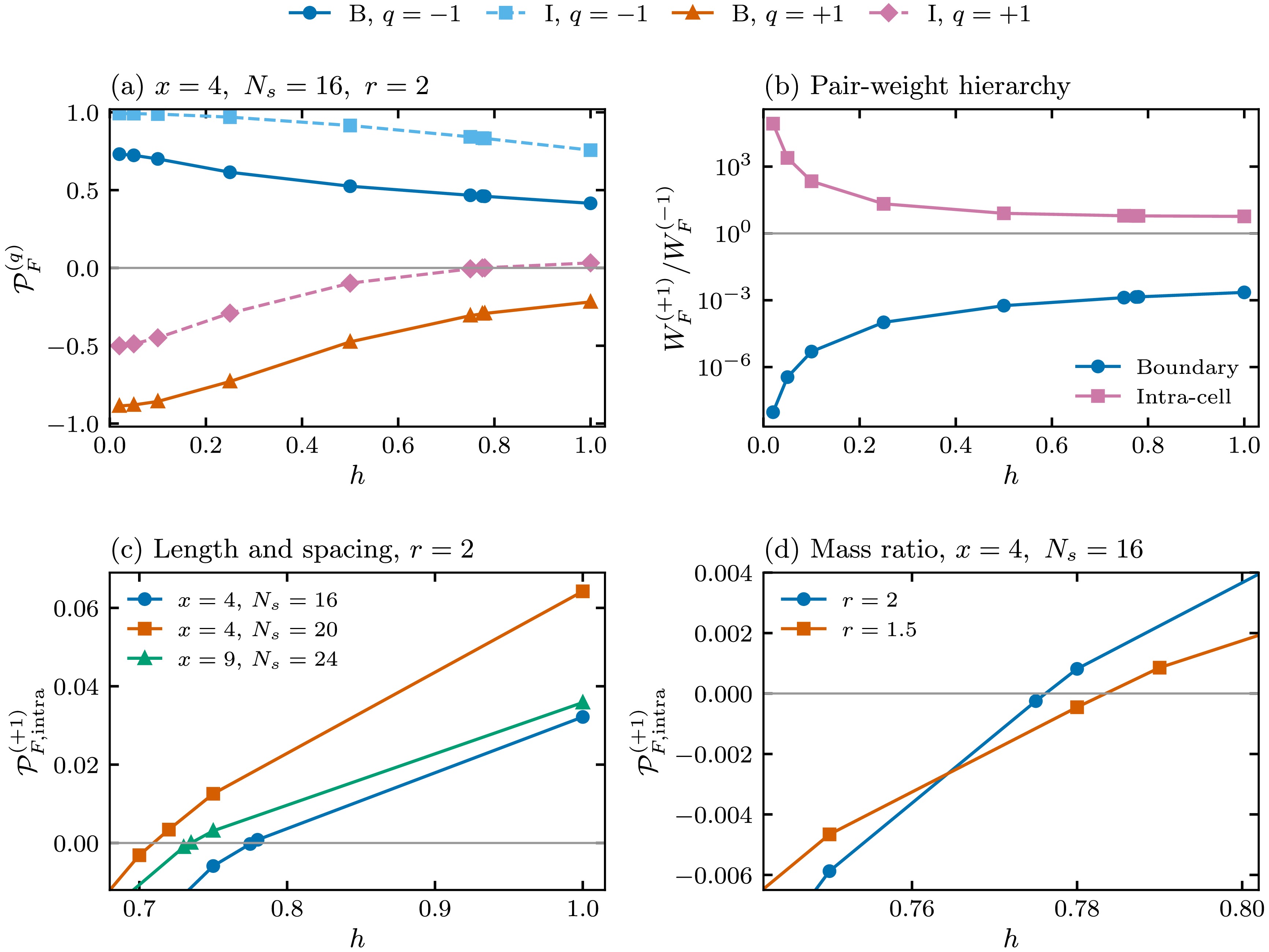
Figure C1. (color online) Hopping interpolation at
$ \theta=\pi $ that connects the atomic reference to the original Hamiltonian. (a) Signed polarizations for both charges and cut classes at$ x=4,N_s=16,r=2 $ ; B denotes a unit boundary, and I denotes the mirror-combined intra-cell cuts. (b) The pair weight ratio retains the opposite hierarchies of the cut classes. (c) Target$ q=+1 $ intra-cell polarization near the crossing for two lengths and two spacings. (d) Comparison for the smaller mass ratio. All axes are dimensionless. Connecting lines are guides to the eye. Conditional values of non-dominant, tiny-weight sectors at$ h<0.02 $ are excluded from the cross-sector comparison.$ x,N_s,r $ $ h_- $ $ h_+ $ $ {\cal{P}}(h_-) $ $ {\cal{P}}(h_+) $ $ \delta_\chi{\cal{P}} $ $ \delta_{\rm{dir}}{\cal{P}} $ $ 4,16,2 $ 0.775 0.78 $ -2.50\times10^{-4} $ $ 8.16\times10^{-4} $ $ 5.28\times10^{-12} $ $ 7.96\times10^{-14} $ $ 4,20,2 $ 0.7 0.72 $ -3.12\times10^{-3} $ $ 3.42\times10^{-3} $ $ 6.80\times10^{-12} $ $ 1.40\times10^{-13} $ $ 9,24,2 $ 0.73 0.735 $ -1.05\times10^{-3} $ $ 1.33\times10^{-5} $ $ 5.69\times10^{-12} $ $ 8.14\times10^{-14} $ $ 4,16,1.5 $ 0.78 0.79 $ -4.53\times10^{-4} $ $ 8.56\times10^{-4} $ $ 1.71\times10^{-11} $ $ 4.79\times10^{-13} $ Table C1. Resolved sign brackets for
$ {\cal{P}}_{F,\mathrm{intra}}^{(+1)} $ . The interval endpoints have opposite signs; no fitted transition point is implied.$ \delta_\chi{\cal{P}} $ denotes the larger adjacent-χ change between the upward and downward hopping continuations, maximized over the two endpoints.$ \delta_{\rm{dir}}{\cal{P}} $ compares these continuations at the final χ. All entries are dimensionless; the endpoint comparisons use$ \chi=256,384 $ . -
Let
$ \lambda_{1,\pm} $ denote the largest eigenvalues of the two subnormalized blocks of$ \rho_A $ , which have traces$ p_\pm $ , and let$ \widetilde\lambda_{1,\pm} $ denote those of the corresponding trace-one blocks. They satisfy$ \lambda_{1,\pm}=p_\pm\widetilde\lambda_{1,\pm} $ and determine the lowest entanglement energies. The difference between the block minima, used here as a derived logarithmic diagnostic, is therefore$ \begin{aligned}[b]D_F =\;&\epsilon_1^{(-1,+1)}-\epsilon_1^{(-1,-1)} =\underbrace{\ln \left(\frac{p_-}{p_+}\right)}_{D_F^{\mathrm{weight}}} +\underbrace{\ln \left(\frac{\widetilde\lambda_{1,-}}{\widetilde\lambda_{1,+}}\right)}_{D_F^{\mathrm{conf}}},\\ D_F^{\mathrm{weight}} =\;&-2\text{artanh} \left({\cal{P}}_F^{(-1)}\right). \end{aligned} $
(D1) Therefore,
$ D_F^{\mathrm{weight}} $ is a monotonic logarithmic representation of the conditional polarization. The smaller contribution,$ D_F^{\mathrm{conf}} $ , compares only the largest eigenvalues of the two normalized blocks and therefore does not characterize their full normalized spectra.The probabilities
$ p_\pm $ refer to the$ q=-1 $ pair defined in Eq. (32). Under flavor exchange,$ D_F $ is odd in η. The block-minimum difference$ D_F $ remains a valid full-spectrum entanglement-energy difference, but Eq. (D1) specifies its role. Across the same 32 unequal-mass states and both cut classes, the normalized block-minimum correction never exceeds$ 1.292$ % of$ |D_F| $ . Consequently, the logarithmic response and its cut contrast are almost entirely determined by the pair-normalized conditional flavor asymmetry at fixed$ Q_A=-1 $ .For completeness, the relative contribution
$ |D_F^{\mathrm{conf}}/D_F| $ has median, mean, and maximum values of$ 0.6527$ %,$ 0.6939$ %, and$ 1.2916$ % at the 32 unit-cell boundaries. After combining reflection-related intra-cell cuts, the corresponding values are$ 0.0619$ %,$ 0.0585$ %, and$ 0.1428$ %. The smaller term is independently resolved over the available increases in bond dimension, but it neither determines the main probability response nor characterizes the full normalized block spectra. -
Across the full six-ratio
$ gL_{\rm{phys}}=8 $ scan, the selected-boundary pair weight is approximately$ 0.35 $ –$ 0.40 $ , whereas the mirror-combined intra-cell value is approximately$ 0.018 $ –$ 0.038 $ . Despite its smaller weight, the intra-cell polarization increases more rapidly and reaches$ 0.61 $ –$ 0.76 $ at$ r=2 $ across the four spacings, compared with$ 0.32 $ –$ 0.42 $ at the unit-cell boundary.The complementary charge pairs have the following weight-ratio ranges over the primary grid:
$\begin{aligned}[b]& 0.00203\leq \frac{W_F^{(+1)}}{W_F^{(-1)}} \leq0.01111 \quad\text{at unit-cell boundaries}, \\& 4.453\leq \frac{W_F^{(+1)}}{W_F^{(-1)}} \leq8.777 \quad\text{intra-cell}.\end{aligned} $
(D2) The two aspects of the response change in opposite directions when the cut is changed. For each unequal-mass state, we compare the selected unit-cell boundary with the arithmetic mean of its reflection-related intra-cell block weights. The resulting ratios are
$ 0.0523\leq \frac{W_{F,\mathrm{intra}}^{(-1)}}{W_{F,\mathrm{boundary}}^{(-1)}} \leq0.1100, \qquad 1.787\leq \frac{{\cal{P}}_{F,\mathrm{intra}}^{(-1)}}{{\cal{P}}_{F,\mathrm{boundary}}^{(-1)}} \leq2.242. $
(D3) Thus, the intra-cell cut retains only about
$ 5$ %–$ 11$ % of the partner-pair probability found at the unit boundary, but it exhibits a larger conditional flavor polarization. The polarization ratio is not constant: across the complete six-ratio families, it decreases systematically from$ 2.176 $ –$ 2.242 $ at$ r=1.125 $ to$ 1.823 $ –$ 1.928 $ at$ r=2 $ . Figure D1 plots the state-matched ratios against r. At every sampled geometry, the weight ratio increases across the available mass ratios, whereas the polarization ratio decreases across the available unequal-mass ratios. The weight suppression and polarization enhancement are therefore parameter-dependent rather than constant cut factors.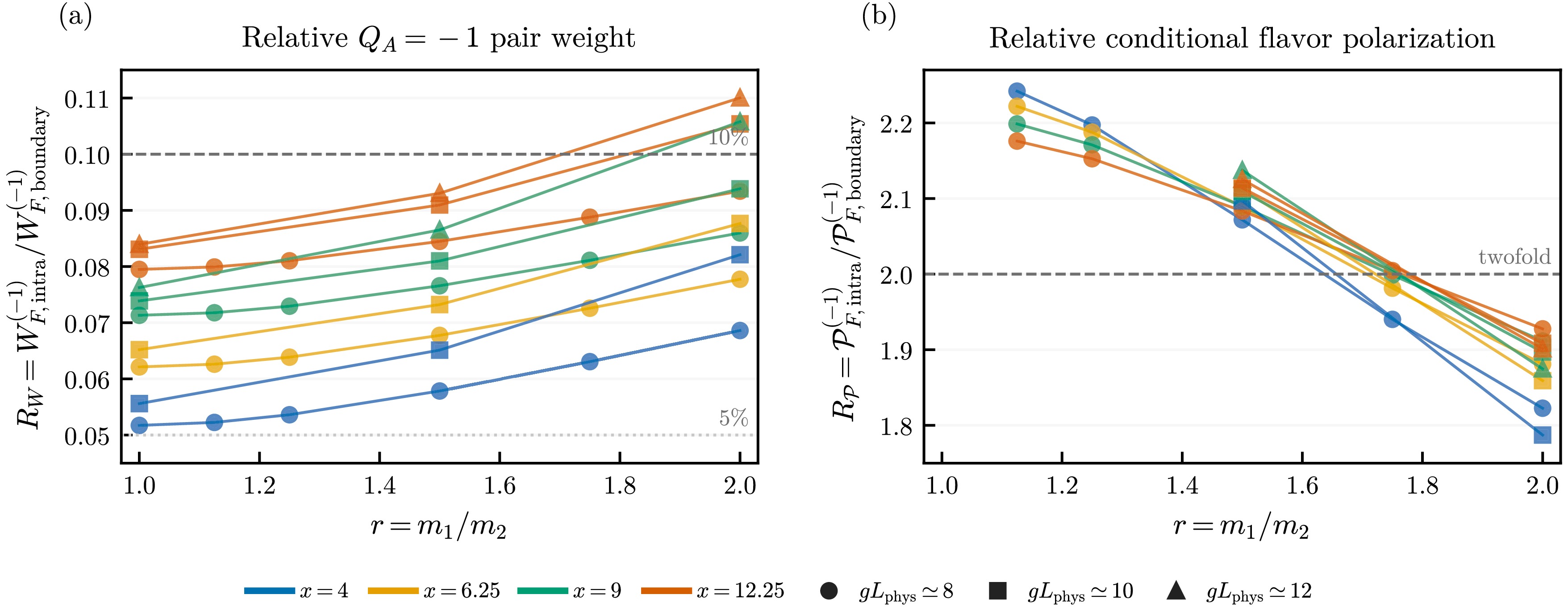
Figure D1. (color online) State-matched intra-to-boundary ratios as functions of mass ratio. Panel (a) shows
$ R_W=W_{F,\mathrm{intra}}^{(-1)}/W_{F,\mathrm{boundary}}^{(-1)} $ for all 42 states, including the equal-mass case. Panel (b) shows$ R_{{\cal{P}}}={\cal{P}}_{F,\mathrm{intra}}^{(-1)}/{\cal{P}}_{F,\mathrm{boundary}}^{(-1)} $ for the 32 unequal-mass states. At$ r=1 $ , flavor symmetry gives$ {\cal{P}}_{F,\mathrm{intra}}^{(-1)}={\cal{P}}_{F,\mathrm{boundary}}^{(-1)}=0 $ , so$ R_{{\cal{P}}} $ is undefined, and no equal-mass point is plotted in panel (b). Color indicates x, marker shape indicates$ gL_{\mathrm{phys}}\simeq8,10,12 $ , and thin lines connect only sampled ratios from the same finite-chain family as visual guides. All plotted quantities are dimensionless.The increase in
$ R_W $ indicates that$ W_{F,\mathrm{intra}}^{(-1)} $ grows by a larger fraction, rather than by a larger absolute amount, than$ W_{F,\mathrm{boundary}}^{(-1)} $ . At unit-cell boundaries, the$ Q_A=-1 $ pair already dominates the non-neutral probability, and its growth accompanies non-neutral broadening. At intra-cell cuts, the initially smaller$ Q_A=-1 $ pair grows, whereas the dominant$ Q_A=+1 $ pair and the total non-neutral probability decrease; this behavior is consistent with a redistribution principally from$ Q_A=+1 $ toward$ Q_A=-1 $ .Define
$ u_c=-D_{F,c}^{\mathrm{weight}}/2=\text{artanh}{\cal{P}}_{F,c}^{(-1)}>0 $ for$ c=\mathrm{boundary},\mathrm{intra} $ and$ r>1 $ , so that$ R_{{\cal{P}}}=\tanh u_{\mathrm{intra}}/ \tanh u_{\mathrm{boundary}} $ . Because$ u_{\mathrm{intra}}>u_{\mathrm{boundary}} $ and$ \tanh u/u $ decreases for$ u>0 $ , this mapping compresses the polarization ratio below the log-odds ratio. The latter also decreases slightly along the sampled path; therefore, the decline in$ R_{{\cal{P}}} $ is not solely a consequence of boundedness. -
Flavor exchange was checked for
$ r=2\leftrightarrow0.5 $ and$ r=1.0625\leftrightarrow\frac{1}{1.0625} $ . The nearly equal calculations were performed with$ (x,N_s,gL_{\rm{phys}},\chi,\ell_\star)=(9,24,8.00,256,12) $ and$ (12.25,28,8.00,256,14) $ . The flavor-invariant spectra agree, whereas the$ F_A $ labels are exchanged. The specified consistency tolerance is$ 10^{-8} $ , and the largest reported reciprocal residual is below$ 2.5\times10^{-9} $ . This tolerance is not a DMRG convergence threshold. The nearly equal points test the expected odd response without defining a precision susceptibility.Write
$ H_{Q,F}(r) $ for the Hamiltonian in total sector$ (Q,F) $ . Flavor swap gives$\begin{aligned}[b]& {\cal{X}}H_{Q,F}(r){\cal{X}}^{-1}=H_{Q,-F} \left(\frac{1}{r}\right),\\& \text{Spec}H_{Q,F}(r)=\text{Spec}H_{Q,-F} \left(\frac{1}{r}\right).\end{aligned} $
(D4) For even-length chains in the neutral
$ L_{-1}=0 $ internal-link realization, the canonical particle–hole reflection$ {\cal{P}}c_{n,\alpha}{\cal{P}}^{-1}=(-1)^n c^\dagger_{N_s-1-n,\alpha} $ maps$ Q_n\to-Q_{N_s-1-n} $ , reflects the hopping and electric-field sums, preserves the staggered mass term, and yields$ {\cal{P}}H_{0,F}(r){\cal{P}}^{-1}=H_{0,-F}(r). $
(D5) This concise mapping is distinct from the one-site-translating staggered charge conjugation discussed in Sec. II.A; it also provides an exact check of the sector construction. The explicit C asymmetry in the open-boundary realization implies that these finite-chain calculations do not test the two-vacuum degeneracy of the C-broken infinite-volume theory.
-
For each charge sector, we evaluate the numerator that determines the sign and the probability outside the selected flavor pair:
$ N_F^{(q)}=p_{q,+1}-p_{q,-1}, \qquad \varepsilon_{\rm{other}}^{(q)} =p_{Q_A}(q)-W_F^{(q)} =\sum\limits_{f\ne\pm1}p_{q,f}. $
(E1) The relative omitted weight is
$ \varepsilon_{\rm{other}}^{(q)}/p_{Q_A}(q) $ . All terms are computed from the complete finite-MPS Schmidt distribution. For$ q=+1 $ , the maxima over the primary states and individual cuts are$ 9.775\times10^{-7} $ in absolute probability and$ 4.737\times10^{-6} $ relative to the charge-sector weight. This bounds the accuracy of representing that sector by its$ F_A=\pm1 $ pair; it is distinct from both the total normalization accuracy and the accuracy of an individual entanglement level.For the 29 final hopping-interpolation states and all three individual cuts, the
$ q=+1 $ maxima are$ 1.725\times10^{-6} $ (relative) and$ 3.393\times10^{-7} $ (absolute). Both occur at the right intra-cell cut for$ (x,N_s,r,h)=(9,24,2,1) $ .For small pair weights, component errors can be amplified in the conditional ratio. Writing
$ a=p_{q,+1} $ and$ b=p_{q,-1} $ gives$ \delta{\cal{P}}_F^{(q)} =\frac{2b\,\delta a-2a\,\delta b}{(a+b)^2} +O(\delta a^2,\delta a\,\delta b,\delta b^2). $
(E2) We therefore compare
$ a,b,N_F^{(q)} $ directly, as well as$ {\cal{P}}_F^{(q)} $ . For the smallest nonzero primary mass imbalance,$ r=1.125 $ , the unit-cell numerator for$ q=+1 $ at$ x=4,N_s=16 $ is$ -3.47646\times10^{-5} $ , and its adjacent-χ change is$ 1.43\times10^{-11} $ . The minimum signal-to-change ratio across all unequal-mass primary numerators for$ q=+1 $ is$ 5.165\times10^4 $ . The signs at the two highest χ values agree throughout. Equal-mass polarizations for$ q=+1 $ have a maximum magnitude of$ 1.38\times10^{-9} $ at unit-cell boundaries and$ 3.02\times10^{-10} $ in the mirror-combined intra-cell class.The additional calculations use four hopping families:
$ (x,N_s,r)=(4,16,2),(9,24,2),(4,20,2),(4,16,1.5) $ , with 11, 6, 6, and 6 sampled hopping values, respectively. Increasing- and decreasing-h continuations are optimized independently through the chosen points, each with an adjacent bond-dimension comparison. Most points use$ \chi=128,256 $ ; the sign-bracket endpoints use$ \chi=256,384 $ . The plotted probabilities use the final increasing-h state. Throughout the manuscript, the hopping-convergence convention is:$ \begin{aligned}[b]& \delta_\chi O =\max\limits_{d\in\{\uparrow,\downarrow\}} \left|O^{d}_{\chi_{\rm{high}}}-O^{d}_{\chi_{\rm{previous}}}\right|,\\& \delta_{\rm{dir}}O =\left|O^\uparrow_{\chi_{\rm{high}}}-O^\downarrow_{\chi_{\rm{high}}}\right|. \end{aligned} $
(E3) The bracket table maximizes each diagnostic over its two endpoints. These comparisons assess direct stability and are not rigorous error bounds.
The target intra-cell
$ q=+1 $ signs and pair weights are resolved at all sampled nonzero hopping values. For the cross-sector sign comparison, we use$ h\ge0.02 $ : below this value, the non-dominant unit-cell$ q=+1 $ probability becomes extremely small (approximately$ 5.1\times10^{-15} $ at$ x=4,N_s=16,r=2,h=0.005 $ ), so its conditional polarization is not used to support a physical sign claim. Across the resolved comparisons,$ q=-1 $ remains positive in both cut classes, and unit-cell$ q=+1 $ remains negative. The non-neutral pair-weight hierarchy is retained at all sampled points.The 29 final hopping states and four matched equal-mass references all satisfy the specified physical convergence checks and the final-stage engine stopping criteria. An earlier
$ \chi=128 $ stage at$ x=9,h=1 $ reached its sweep limit; the adopted higher-χ stage was converged separately. For very small h, the top-level test uses the available nonzero Schmidt levels; it neither infers missing levels nor replaces them with zeros. -
Along the fixed-geometric-mean mass path, both the common mass
$ m=(m_1+m_2)/2 $ and the mass difference$ \delta m=(m_1-m_2)/2 $ vary. Four equal-mass states$ (m,m) $ , matched at$ (x,N_s)=(4,16),(9,24) $ and$ r=1.5,2 $ , are used to separate the two finite-difference terms:$ \begin{aligned}[b]& O(m+\delta m,m-\delta m)-O(m_0,m_0) \\=\;&[O(m,m)-O(m_0,m_0)]\\& +[O(m+\delta m,m-\delta m)-O(m,m)], \end{aligned} $
(E4) where
$ m_0=0.5g $ . The common mass is$ 0.510310g $ for$ r=1.5 $ and$ 0.530330g $ for$ r=2 $ . Table E3 lists the terms along this specified comparison path.Diagnostic Maximum over final states Criterion $ v_E/(g^2) $ $ 1.45\times10^{-10} $ $ 10^{-6} $ Discarded weight $ 3.00\times10^{-12} $ $ 10^{-6} $ $ |\Delta_\chi E|/g $ $ 6.99\times10^{-8} $ $ 10^{-6} $ $ \max|\Delta_\chi\epsilon| $ $ 4.53\times10^{-4} $ $ 10^{-3} $ Bulk-window change $ 1.00\times10^{-7} $ $ 10^{-3} $ Table E2. Numerical diagnostics for the 33 final states used in the hopping and matched-mass calculations (29 hopping points and four equal-mass references). The variance is reported per site. The discarded weight is maximized over the final-stage sweeps. Spectral changes are compared using up to 20 available nonzero Schmidt levels without applying a probability cutoff. At very small hopping, fewer levels may be available; absent levels are not treated as converged. All final stages satisfy the engine stopping criteria independently of these physical checks.
x r Cut $ W_F^{(-1)} $ $ W_F^{(+1)} $ ($ 10^{-3} $ )$ p_{Q_A\ne0} $ Mean Split Mean Split Mean Split 4 1.5 B −0.0046 +0.013 −0.00827 −0.0319 −0.00575 +0.0141 4 1.5 I −0.000761 +0.00341 −0.239 −3.29 −0.001 −0.000143 4 2 B −0.0133 +0.0372 −0.0252 −0.0857 −0.0166 +0.0403 4 2 I −0.00214 +0.00974 −0.783 −9.25 −0.00294 −0.00021 9 1.5 B −0.00365 +0.00942 −0.0149 −0.0847 −0.00488 +0.0107 9 1.5 I −0.000906 +0.0033 −0.0105 −3.35 −0.000903 −0.000446 9 2 B −0.0106 +0.027 −0.0469 −0.231 −0.0141 +0.0306 9 2 I −0.00256 +0.00942 −0.127 −9.45 −0.00267 −0.00114 Table E3. Decomposition of the matched mean mass. B and I denote the selected unit-cell boundary and the mean adjacent intra-cell cut, respectively. Mean and Split are the two terms in Eq. (E4); their sum gives the total change.
$ gL_{\rm{phys}}=8 $ , with$ N_s=16 $ at$ x=4 $ and$ N_s=24 $ at$ x=9 $ . All changes are dimensionless, and the$ W_F^{(+1)} $ columns are reported in units of$ 10^{-3} $ .$ N_s $ r $ |v_E|/g^2 $ $ |\Delta_\chi E|/g $ final discarded top-20 $ \epsilon $ drift16 2 $ 2.10\times10^{-13} $ $ 3.24\times10^{-10} $ $ 9.67\times10^{-15} $ $ 7.97\times10^{-6} $ 20 2 $ 8.87\times10^{-13} $ $ 1.09\times10^{-9} $ $ 3.16\times10^{-14} $ $ 1.30\times10^{-5} $ 16 1.5 $ 3.09\times10^{-13} $ $ 4.32\times10^{-10} $ $ 1.22\times10^{-14} $ $ 1.15\times10^{-5} $ Table E4. Numerical controls for the background scan, maximized over the adopted angles at
$ x=4 $ . Variance per site is reported in units of$ g^2 $ , and energy drift is reported in units of g; discarded weights and level drifts are dimensionless. All adopted$ \chi=256 $ states satisfy the engine stopping criteria. Tiny negative raw variances caused by cancellation are retained in the records; their absolute magnitudes are reported here. The representative energy and spectrum comparisons use the increasing-angle ladder, whereas the extensions maximize over both directions.At the unit boundaries, the mass-difference term increases
$ W_F^{(-1)} $ and offsets a negative common-mass term. Within a unit cell, it increases$ W_F^{(-1)} $ but decreases$ W_F^{(+1)} $ . The common-mass term accounts for most of the total non-neutral decrease along the original path: at$ r=2 $ , its shares are$ 93.34$ % for$ x=4 $ and$ 70.14$ % for$ x=9 $ . The equal-mass reference polarizations have a maximum magnitude of$ 3.42\times10^{-10} $ . Changing only the common mass does not produce flavor-odd polarization, although it changes the response to a mass difference. -
At fixed
$ gL_{\rm{phys}}=8 $ and$ r=2 $ , increasing x from 4 to 12.25 changes the weight of the unit-boundary$ q=-1 $ mode from$ 0.376732 $ to$ 0.392625 $ , while its polarization decreases from$ 0.415256 $ to$ 0.317249 $ . Within the cell, the$ q=+1 $ weight increases from$ 0.150162 $ to$ 0.212193 $ , and its polarization increases from$ 0.032165 $ to$ 0.038063 $ . At fixed spacing, comparisons across lengths preserve the signs and weight hierarchy but change their amplitudes, as shown in Fig. E2.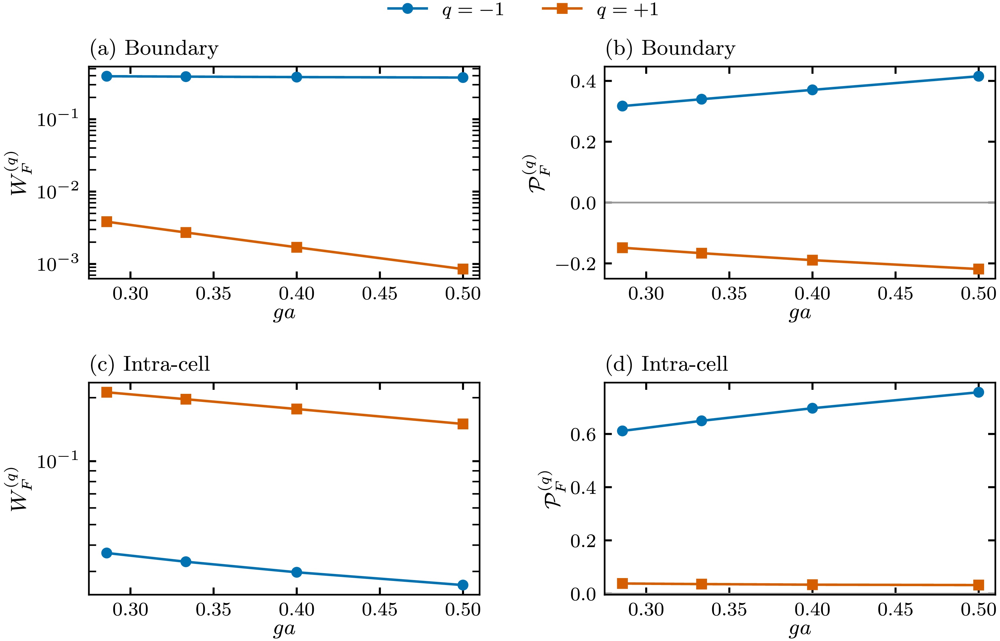
Figure E1. (color online) Dependence on lattice spacing at
$ \theta=\pi $ ,$ h=1 $ ,$ r=2 $ , and fixed$ gL_{\rm{phys}}=8 $ . The four spacings correspond to$ x=4,6.25,9,12.25 $ and$ N_s=16,20,24,28 $ . Rows distinguish the cut classes; columns show pair weights on a logarithmic scale and signed polarizations. All axes are dimensionless, with$ ga=1/\sqrt{x} $ .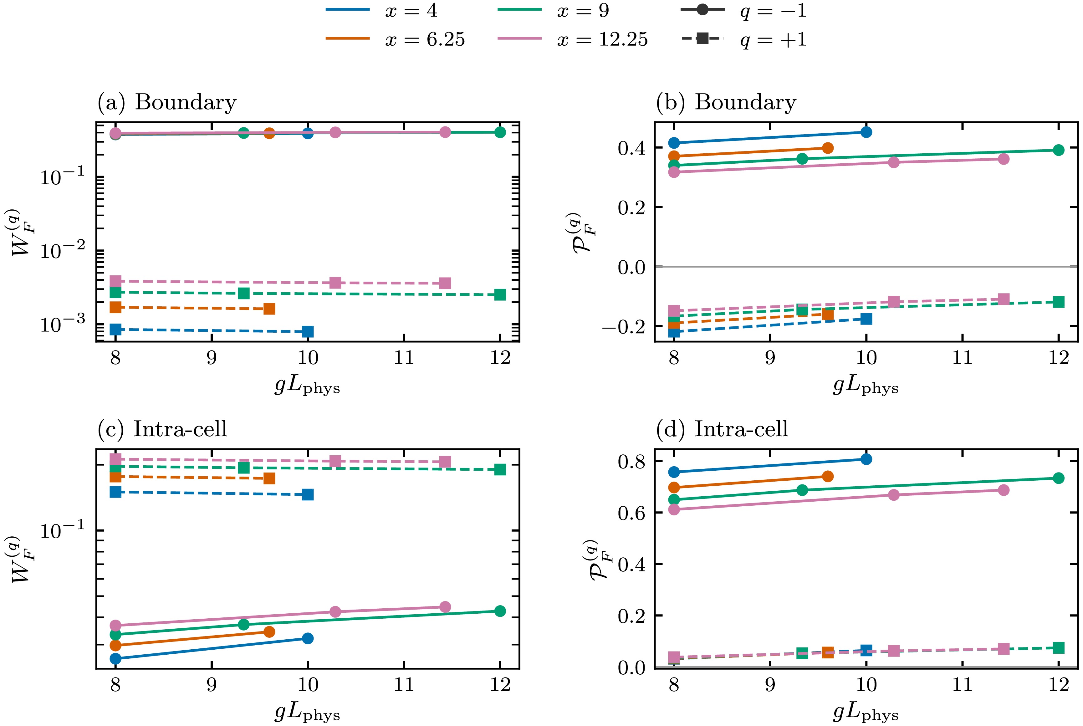
Figure E2. (color online) Length dependence at
$ \theta=\pi $ ,$ h=1 $ , and$ r=2 $ . Colors denote fixed values of x, and line styles distinguish$ q=\pm1 $ . The horizontal coordinate is the actual dimensionless length,$ gL_{\rm{phys}}=N_s/\sqrt{x} $ . Rows correspond to cut classes, whereas columns show dimensionless pair weights and polarizations. Lines connect the available finite-chain results.The
$ N_s=18,x=4,r=2 $ reversed-centering control yields$ {\cal{P}}_F^{(+1)}=+0.052609 $ at the exactly central intra-cell cut and$ -0.197511 $ at the averaged neighboring unit-cell boundaries. The corresponding changes between adjacent χ values are$ 4.18\times10^{-9} $ and$ 2.38\times10^{-8} $ , respectively. This result complements the original$ q=-1 $ centering check in Table B4. -
These interpolations use independent increasing- and decreasing-parameter continuations and explicit componentwise convergence checks, with
$ \mathrm{svd\_min}=10^{-13} $ for the background scans.The representative
$ (x,N_s,r)=(4,16,2) $ scan uses$ \theta/\pi=0,0.5,0.75,0.875,0.89,0.9,1 $ . The length extension uses$ 0,0.5,0.8,0.82,0.84,0.9,1 $ , and the$ r=1.5 $ extension uses$ 0,0.5,0.875,0.89,0.9,1 $ . Each new angle is evaluated with two continuation directions and$ \chi=128,256 $ ; the existing$ \theta=\pi $ checkpoints are independently remeasured rather than recomputed. The two extensions add 44 optimization stages, with 13 adopted physical parameter points, including the two reused endpoints. The final states are the increasing-angle,$ \chi=256 $ states; all three cuts and both q sectors are included in the comparisons.Every adopted checkpoint is reloaded, its conventions and canonical occupations are checked, and its complete joint distribution is reconstructed. Direct flavor-occupation counting agrees with the charge-label reconstruction. Subsystem first moments computed from Schmidt probabilities agree with the site-density sums. All stored Schmidt values contribute, without applying the low-level table threshold. For the extension scans, the maximum target intra-cell
$ q=+1 $ adjacent-χ changes are$ 4.15\times10^{-10} $ at$ N_s=20,r=2 $ and$ 1.47\times10^{-10} $ at$ N_s=16,r=1.5 $ ; their maximum opposite-continuation changes are$ 1.01\times10^{-13} $ and$ 4.19\times10^{-13} $ . The absolute numerator exceeds the larger observed change by at least$ 8.53\times10^6 $ and$ 1.06\times10^7 $ , respectively. Here, the adjacent-χ drift is maximized over the two directions, as in Eq. (E3).The largest relative probability omitted by the
$ F_A=\pm1 $ representation of$ q=+1 $ , across all angles and individual cuts, is$ 2.84\times10^{-7} $ for the representative scan,$ 3.20\times10^{-7} $ for the longer chain, and$ 3.17\times10^{-7} $ for the smaller mass ratio. The corresponding absolute maxima are$ 6.90\times10^{-8} $ ,$ 6.49\times10^{-8} $ , and$ 7.72\times10^{-8} $ . These values provide explicit omission bounds for the finite-MPS distributions, rather than machine-zero claims or bounds on unsampled states.The additional
$ N_s=4 $ matrix and canonical-sector ED comparisons cover$ \theta/\pi=0,0.5,1 $ at both mass ratios. They verify the full MPO, directional signs, and joint probabilities independently of the long-chain continuation. The exact source identity and the directional costs are also checked against diagonal matrix elements. For the free control, the correlation-matrix counting probabilities agree with direct Slater-probability sums to within$ 4.4\times10^{-15} $ ; the decoupled electric control is solved in the two independent fixed-particle-number spaces. The marginal product for the full state is evaluated from the same complete interacting Schmidt distribution and is never substituted for a distinct Hamiltonian state. -
We repeat the background scan at
$ (x,N_s,r)=(4,20,2) $ and$ (4,16,1.5) $ , reusing the corresponding original$ \theta=\pi $ states. Each new state provides data for both charge sectors, the two single-flavor marginals, and both flavor-flux profiles at the three central cuts. Figure E3 and Table E5 show that the mechanism extends beyond the representative length and mass ratio.
Figure E3. (color online) Targeted background-angle extensions at fixed
$ x=4 $ ,$ m_{\rm{geom}}/g=0.5 $ , and$ h=1 $ , each using its left-adjacent intra-cell cut,$ \ell=N_s/2-1 $ . (a) Actual positive-charge conditional polarization. (b) Ratio of single-flavor positive-to-neutral odds,$ R_2/R_1 $ ; values below unity indicate that the light-flavor odds are lower than the heavy-flavor odds. Colors and markers distinguish the three finite-chain families. All axes are dimensionless. Symbols denote computed points; lines do not resolve zeros beyond the sampled brackets.$ N_s $ r bracket in $ \theta/\pi $ heavy (%) light (%) $ \delta\overline L_1 $ $ \delta\overline L_2 $ 16 2 $ (0.89,0.90) $ 20.05 50.37 $ -0.031252 $ $ -0.107294 $ 20 2 $ (0.82,0.84) $ 20.01 52.70 $ -0.030939 $ $ -0.117343 $ 16 1.5 $ (0.89,0.90) $ 25.54 43.62 $ -0.041886 $ $ -0.086291 $ Table E5. Background-angle comparison at fixed
$ x=4 $ and$ h=1 $ . The$ N_s=16,r=2 $ row serves as the representative scan. The two suppression columns report$ 100[1-p(\pi)/p(0)] $ for the actual heavy- and light-flavor events; the final two columns give the induced mean bare-flux contributions defined in Eq. (43). All entries are dimensionless; suppression is expressed as a percentage, and$ N_s $ is a site count.Extending the chain at fixed spacing and
$ r=2 $ shifts the actual sign-change bracket to$ 0.82<\theta_*/\pi<0.84 $ , below the$ N_s=16 $ interval. This conclusion follows from direct opposite-sign points, not from the larger positive endpoint. At$ N_s=20 $ , the heavy- and light-flavor event probabilities decrease by$ 20.01$ % and$ 52.70$ %, respectively, from zero background to π. The light flavor again provides the larger opposite-sign mean flux response,$ -0.11734277 $ compared with$ -0.03093877 $ . At$ \theta/\pi=0.82 $ , its marginal reconstruction is positive,$ +0.00060057 $ , but its joint polarization remains negative,$ -0.00289535 $ . Thus, the distinction between individual responses and joint correlations persists.At the smaller ratio
$ r=1.5 $ , the actual polarization changes from$ -0.11893214 $ to$ +0.01957762 $ , with the resolved bracket$ 0.89<\theta_*/\pi<0.90 $ . This overlaps the representative bracket for$ r=2 $ and does not determine a direction of mass-ratio-induced movement. The two actual event probabilities decrease by$ 25.54$ % and$ 43.62$ %, and the light-flavor mean flux response remains larger in magnitude. At$ \theta/\pi=0.89 $ , the marginal product gives$ +0.00141711 $ , whereas the actual polarization is$ -0.00068789 $ . Both extensions therefore reproduce unequal suppression and correlation-sensitive crossing, rather than merely positive endpoints.Flavor-exchange oddness yields a smooth near-equal-mass polarization that is proportional to
$ \eta=\ln r $ at leading order, with a background-dependent coefficient. Its amplitude can vanish as$ \eta\to0 $ without requiring its zero to approach π. The two mass ratios considered here do not determine that limit. Likewise, the two lengths considered here demonstrate a shift over a finite interval, not a length-scaling law. -
The control in Eq. (44) retains the background source while removing
$ K\sum\nolimits_nL_n^2 $ , including both self-energy and cross terms. We keep$ x=4 $ ,$ N_s=16 $ ,$ r=2 $ ,$ h=1 $ ,$ m_{\rm{geom}}/g=0.5 $ , and the original lattice mass shift. With$ \tau=\theta/\pi $ , Gauss's law transforms the source into the one-body potential$ K\tau(N_s-1-j) $ at site$ j $ , up to a state-independent constant. For each flavor, we fill its eight lowest single-particle orbitals. If$ \nu_{\alpha,j} $ denote the restricted correlation-matrix eigenvalues for flavor α, the corresponding subsystem number probabilities are the coefficients of$ \prod_j(1-\nu_{\alpha,j}+z\nu_{\alpha,j}) $ [27]. The distributions of the two flavors factorize, giving the joint charges through Eq. (20).Figure E4 pairs the conditional polarization with the corresponding event weight. The source-retained control changes sign in
$ (0.44,0.45) $ and$ (0.875,0.88) $ , with numerical zeros near$ \tau=0.4473 $ and$ 0.8795 $ . Thus, the heavy-flavor preference occurs at intermediate source strength but does not persist to$ \theta=\pi $ . At that endpoint, the charge distribution is concentrated near$ Q_A=-2 $ , with probability about$ 0.744 $ , whereas the full model has$ p_{Q_A=0}\simeq0.819 $ . The measured$ \sum\nolimits_n\langle L_n^2\rangle $ is about$ 53.54 $ without quadratic electric energy,$ 5.64 $ with self-energies and source, and$ 5.13 $ in the full model. These changes in the distributions explain why the event weights must accompany the conditional ratios.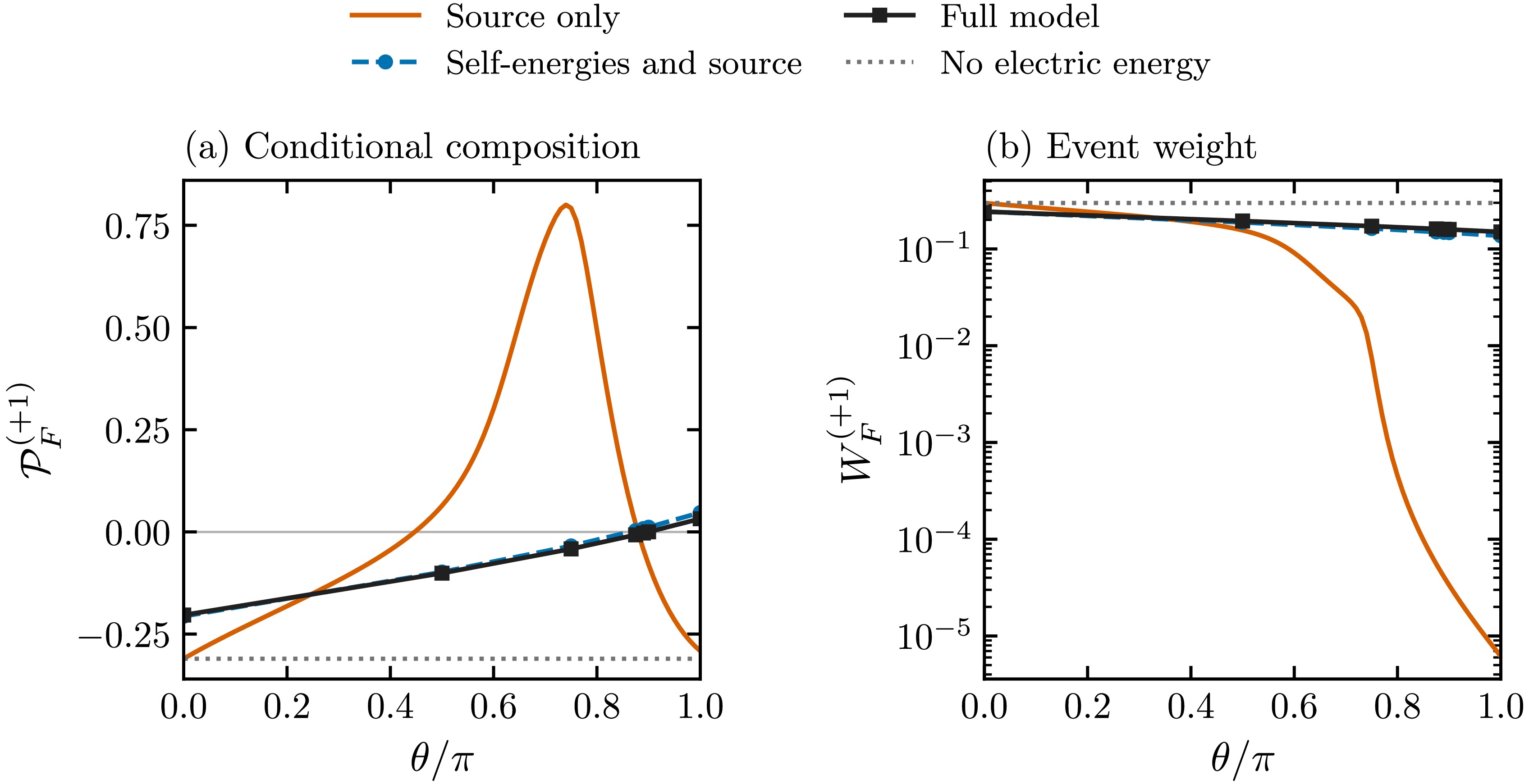
Figure E4. (color online) Background source and quadratic electric energy for fixed
$ x=4,N_s=16,r=2,m_{\rm{geom}}/g=0.5,h=1 $ , with intra-cell cut$ \ell=7 $ and$ q=+1 $ . (a) Signed flavor polarization. (b) Pair-event weight on a logarithmic scale. The source-retained curve uses 102 single-particle solutions; symbols for the self-energy control and the full model denote seven sampled angles, connected as guides. The horizontal dotted reference removes all electric energy, including the source contribution. All axes are dimensionless. The two sign changes in the source-retained control indicate conditional composition crossovers, not phase transitions.The larger mean response of the light flavor does not, by itself, imply a heavy-flavor preference. In the source-retained control, its induced mean bare flux is approximately
$ -0.909 $ , compared with$ -0.813 $ for the heavy flavor, yet the endpoint remains light-flavor favored. Writing the actual event survival fractions as$ S_H(\theta)=p_{+1,+1}(\theta)/p_{+1,+1}(0) $ and$ S_L(\theta)=p_{+1,-1}(\theta)/p_{+1,-1}(0) $ , heavy-flavor dominance requires$ \frac{S_H(\theta)}{S_L(\theta)}>\frac{p_{+1,-1}(0)}{p_{+1,+1}(0)}. $
(E5) At
$ \theta=\pi $ , the source-retained control gives$ 1.042<1.899 $ , whereas the full model gives$ 1.611>1.511 $ . This probability identity distinguishes the change in composition from the magnitude of the mean flux response.The source-retained probabilities were independently verified using complete Slater probability sums and fixed-number Fock-space ED at nine angles, including both sign brackets. The marginal probabilities agree within
$ 2.1\times10^{-14} $ , and the six charge–cut polarizations agree within$ 5.3\times10^{-12} $ . The maximum relative weight outside$ F_A=\pm1 $ for the displayed$ q=+1 $ pair is$ 2.3\times10^{-5} $ over the scan. The self-energy control was independently recomputed, and the seven full-model states were re-evaluated from their saved Schmidt spectra and occupations. Their finite-χ precision remains that reported in Appendix E.4.
Ordering of the entanglement spectrum and flavor polarization in the two-flavor Schwinger model at the vacuum angle θ = π
- Received Date: 2026-08-17
- Available Online: 2027-02-01
Abstract: On finite open staggered chains of the two-flavor Schwinger model at vacuum angle $\theta=\pi$, we resolve the joint Schmidt distribution $p_{Q_A,F_A}$, labeled by the subsystem gauge charge $Q_A$ and flavor imbalance $F_A$. Defining the total weight $W_F^{(q)}=p_{q,+1}+p_{q,-1}$ and the conditional polarization ${\cal{P}}_F^{(q)}=(p_{q,+1}-p_{q,-1})/W_F^{(q)}$, we find that changing the staggered cut reverses the hierarchy of non-neutral pair weights: $W_F^{(-1)}>W_F^{(+1)}$ at unit-cell boundaries, whereas $W_F^{(+1)}>W_F^{(-1)}$ at intracell cuts. The signed polarization further shows that positive charge fluctuations at intracell cuts can favor the heavier flavor despite its larger bare excitation cost. At fixed masses, hopping, and geometry, increasing the background field suppresses $p_{+1,-1}$ more strongly than $p_{+1,+1}$, driving ${\cal{P}}_F^{(+1)}$ through zero and overturning the initial light-flavor advantage. Matched Hamiltonian controls show that the external source alone can produce ${\cal{P}}_F^{(+1)}>0$ at intermediate $\theta$, while electric self-energies sustain an appreciable $W_F^{(+1)}$ with ${\cal{P}}_F^{(+1)}>0$ at $\theta=\pi$; direct interflavor coupling weakens this preference and delays the crossing. Thus, symmetry resolution distinguishes gauge-sector ordering from flavor composition and reveals why a lower bare excitation cost need not determine the flavor composition of a charged vacuum fluctuation.



 DownLoad: