Relativistic Proton-Neutron Quasiparticle-Vibration Coupling Theory with Localized Exchange Terms and Tensor Couplings for Gamow-Teller Resonances and β Decay

Charge-exchange excitations probe the spin-isospin dynamics of atomic nuclei [1–3]. Among charge-exchange modes, Gamow-Teller (GT) transitions are induced by the spin-isospin operator $ \boldsymbol{\sigma}\tau_{\pm} $, which converts a neutron into a proton or vice versa and carries spin transfer $ \Delta S=1 $ without orbital-angular-momentum transfer ($ \Delta L=0 $). The resulting GT strength distributions are sensitive to the shell structure and the spin-isospin components of the nuclear effective interaction [1, 2, 4]. At higher excitation energies, a substantial part of the GT strength is concentrated in the Gamow-Teller resonance (GTR) [5]. Experimentally, charge-exchange reactions such as $ (p,n) $ and $ ({}^{3}\mathrm{He},t) $ can probe GT strength across the resonance region, allowing the GTR centroid and width to be extracted [1, 2, 4].

Complementary to charge-exchange reactions, which are mainly used to study the GTR, β decay provides access to the low-energy GT response. For $ \beta^- $ decay within the allowed-transition approximation, only GT$ ^- $ transitions within the energy window set by the $ Q_{\beta} $ value contribute to the decay rate, and the phase-space factor strongly favors states at lower excitation energies. Consequently, the β-decay half-life is determined by the GT strength distribution within the $ Q_{\beta} $ window [1, 4, 6].

A unified microscopic framework that describes both the GTR and the low-energy GT response relevant to β decay is therefore essential. Various microscopic approaches have been employed to describe GT excitations and β decay, such as the shell model [6, 7], ab initio many-body methods [8–11], and the quasiparticle random-phase approximation (QRPA) [3, 12]. The proton-neutron QRPA (pnQRPA) provides a computationally tractable approach to systematic studies across the nuclear chart [13–15]. In pnQRPA, the GT response arises from the coherent mixing of proton-neutron two-quasiparticle configurations through the residual interaction. In self-consistent QRPA formulations, the residual interaction is derived from the same energy density functional used in the ground-state calculation, which is particularly valuable for systematic extrapolations toward nuclei far from stability [3, 14]. Such formulations have been developed within nonrelativistic Skyrme and Gogny frameworks [16–19] and within relativistic pnQRPA [20–22].

Covariant density functional theory provides a Lorentz-covariant description of nuclei and naturally generates the nuclear spin-orbit coupling [12, 23, 24]. Based on covariant density functionals, relativistic pnQRPA has been widely used in studies of the GT resonance and β decay [14, 20, 21]. However, relativistic pnQRPA models based on relativistic Hartree-Bogoliubov (RHB) theory face two limitations. First, because Fock terms are absent, the pion does not contribute at the mean-field level, although pion exchange remains important for spin-isospin excitations. Hence, the coupling strength of the corresponding channel in the residual pnQRPA interaction, e.g., the Landau-Migdal term for meson-exchange pnQRPA [20, 21] or the isovector-pseudovector coupling channel for point-coupling pnQRPA [25], is not constrained by ground-state properties [26]. Instead, it is typically adjusted to match the experimental GTR energy using a reference nucleus such as $ ^{208} $Pb for calibration. Consequently, these implementations are not fully self-consistent in the charge-exchange channel. Second, commonly used functionals generally have a relatively low Landau effective mass, leading to a sparse single-particle spectrum around the Fermi surface. At the pnQRPA level, the resulting higher energies of relevant two-quasiparticle configurations can place the associated GT strength at higher excitation energies, thereby reducing its contribution to the β-decay rate and leading to overestimated half-lives [21, 27].

The first limitation can be addressed by restoring exchange contributions. Relativistic Hartree-Fock and Hartree-Fock-Bogoliubov theories explicitly include nonlocal Fock terms, which yield a non-zero π contribution already at the mean-field level. Accordingly, the coupling strength in this channel is determined from ground-state properties and subsequently adopted in the spin-isospin residual interaction of the corresponding pnQRPA [22, 26, 28]. Explicit treatment of these nonlocal terms, however, is computationally demanding and hinders large-scale calculations across the nuclear chart. For zero-range point-coupling interactions, the Fierz transformation recasts the exchange contributions into local direct channels [29]. By employing this transformation, Fock terms can be incorporated into local functionals, and spin-isospin excitation energies have been shown to be properly described without readjusting the coupling strength in the residual interaction [30]. The recently proposed point-coupling PCF-PK1 functional follows the same spirit: it includes exchange terms localized via the Fierz transformation while retaining the computational efficiency of the RHB framework [31]. The second limitation can be alleviated either by tensor couplings [21, 31] or by an energy-dependent nucleonic self-energy [27, 32]; both mechanisms can raise the single-particle level density near the Fermi surface, thus increasing the Landau effective mass. In fact, PCF-PK1 raises the Landau effective mass to $ M^*_L = 0.85 m_{N} $ through an isoscalar tensor coupling. Benefiting from these two features, a pnQRPA model based on PCF-PK1 has been constructed. This model demonstrates that localized exchange terms remove the phenomenological tuning of the charge-exchange residual interaction, while the tensor coupling improves β-decay half-lives via the enhanced Landau effective mass ¹. However, for semimagic nuclei (e.g., Ni and Sn isotopes), the predicted half-lives remain systematically longer than the measured half-lives.

The remaining discrepancies reflect the restriction of pnQRPA to two-quasiparticle configurations, which omits correlations responsible for GT spreading [33, 34] and can misplace the low-energy strength relevant to β decay [35]. Isoscalar proton-neutron pairing can lower GT excitation energies within pnQRPA [16, 21], but its effect depends strongly on the nucleus and corresponding shell structure [36]. A unified description of the GTR and β decay therefore requires correlations beyond pnQRPA.

Within the nonrelativistic Skyrme energy density functional framework, the subtracted second random-phase approximation (SSRPA) explicitly couples one-particle-one-hole configurations to two-particle-two-hole (2p-2h) configurations and has been applied to GT strength quenching [37, 38] and β-decay half-lives [39, 40]. The role of tensor interactions has also been investigated in SSRPA calculations of β decay [39] and magnetic dipole excitations [41]. Particle-vibration coupling (PVC) incorporates 2p-2h correlations through the coupling of particle-hole configurations to collective phonons, with phonon selection reducing the computational cost. The Skyrme random-phase approximation (RPA) plus PVC model has successfully described GT spreading [42, 43] and the β-decay half-lives of doubly magic nuclei [35]. Its extension to superfluid nuclei, proton-neutron quasiparticle-vibration coupling (pnQPVC), couples proton-neutron two-quasiparticle configurations to non-charge-exchange phonons. This approach has been used to study the GT response of $ ^{120} $Sn [44], as well as the interplay between PVC and pairing effects on β-decay half-lives of Ni and Sn isotopes [36]. Very recently, QPVC has also been implemented with the deformed Skyrme proton-neutron finite-amplitude method [45].

Within covariant density functional theory, PVC effects on charge-exchange GT and spin-dipole excitations have been investigated in closed-shell nuclei using the relativistic time-blocking approximation (RTBA) [46, 47]. By including pairing correlations, this method was extended to the proton-neutron relativistic quasiparticle time-blocking approximation (pn-RQTBA), enabling the description of GT spreading and β-decay half-lives in open-shell nuclei [48]. Subsequent developments incorporated charge-exchange phonons [49], time-reversed particle-vibration loops and ground-state correlations [50], finite-temperature effects [51], and the inclusion of first-forbidden transitions in β-decay studies [52]. However, these implementations are based on the Hartree approximation, where the absence of explicit Fock terms requires a phenomenologically adjusted zero-range Landau-Migdal interaction in the charge-exchange channel [47, 48, 52]. Moreover, these calculations mainly employed a meson-exchange NL3 parameterization, which has a relatively low Landau effective mass [27, 32]. These features motivate a relativistic QPVC framework incorporating exchange terms localized through the Fierz transformation, as well as tensor couplings.

In this work, we develop a fully self-consistent relativistic pnQPVC model based on the PCF-PK1 point-coupling density functional. Its ground state is obtained within the localized relativistic Hartree-Fock-Bogoliubov (RHFB) theory. Through the Fierz transformation, the charge-exchange particle-hole residual interaction is determined self-consistently without phenomenological adjustment. The charge-exchange pnQRPA states, non-charge-exchange QRPA phonons, and quasiparticle-vibration coupling vertices are constructed consistently from the same particle-hole and particle-particle interactions. We apply the relativistic pnQPVC model to the GT$ ^- $ strength distributions of $ ^{116-134}\mathrm{Sn} $ and the $ \beta^- $-decay half-lives of neutron-rich Ni and Sn nuclei as well as the $ N=50 $ and $ N=82 $ isotonic chains.

The article is organized as follows. Section II presents the localized RHFB ground-state theory and pnQPVC formalism, including the GT strength function and β-decay half-lives. Section III specifies the numerical setup and examines numerical convergence. Section IV discusses the GT response and β-decay half-lives, where the contributions of the isovector-tensor (tT) and isovector-pseudovector (tPV) channels are analyzed in detail. Section V summarizes the main conclusions.

The nuclear ground state is obtained from the localized relativistic Hartree-Fock-Bogoliubov (RHFB) model, which also gives the canonical basis. Based on this foundation, non-charge-exchange QRPA phonons and charge-exchange pnQRPA states are constructed separately. The pnQRPA plus pnQPVC theory explicitly incorporates the coupling between quasiparticles and phonons and is employed to calculate GT strength distributions and $ \beta^- $-decay half-lives.

The covariant point-coupling Lagrangian density for the nuclear system comprises the free-nucleon, four-fermion point-coupling, derivative, and electromagnetic terms [31]:

with

Here, ψ and $ m_N $ denote the nucleon field and nucleon mass, respectively, and $ \bar\psi=\psi^\dagger\gamma^0 $ represents the adjoint spinor. The symbol e signifies the charge unit, while $ A^\mu $ and $ F_{\mu\nu} $ are the electromagnetic four-potential and field-strength tensor, respectively. The isospin matrices are denoted by $ \boldsymbol\tau $, with $ \tau_3 $ as their third component. The derivative term is included only in the isoscalar-scalar channel, with $ \delta_{\rm S} $ representing its coupling constant.

The coefficients $ \alpha_\chi $ in Eq. (2b) represent the coupling constants of the four-fermion point-coupling terms. The channel label χ specifies a product $ (\mathcal O\Gamma)_\chi $, where $ \mathcal O\in\{1,\boldsymbol\tau\} $ denotes the isoscalar and isovector channels, respectively, and $ \Gamma\in\{1,\gamma_\mu,\sigma_{\mu\nu},\gamma_5,\gamma_5\gamma_\mu\} $ corresponds to the scalar (S), vector (V), tensor (T), pseudoscalar (PS), and pseudovector (PV) channels, respectively. The combinations of $ \mathcal O $ and Γ define ten channels, ordered as

The prefix "t" denotes the corresponding isovector channels: tS, tV, tT, tPS, and tPV. Here, $ \sigma_{\mu\nu}=\mathrm{i}[\gamma_\mu,\gamma_\nu]/2 $.

The Hamiltonian is derived from a Legendre transformation of the Lagrangian density in Eq. (1). Within the Hartree-Fock (HF) approximation, its expectation value in the HF ground state gives the energy density functional:

where ρ denotes the normal density. The four-fermion contribution includes both Hartree and Fock terms, i.e., $ E^{\rm 4f} = E_{\rm H} + E_{\rm F} $. Under this HF approximation, we denote the coupling constants as $ \alpha_\chi^{\rm HF} $, where χ represents the coupling channels as shown in Eq. (3). In the present work, exchange terms are retained only for $ E^{\rm 4f} $; the derivative and electromagnetic terms are treated without exchange contributions.

Through the Fierz transformation, the exchange contribution $ E_{\rm F} $ can be reformulated as a sum of direct contributions [29–31]. We denote the corresponding redefined coupling constants as $ \alpha_{\chi} $. The constants $ \alpha_{\chi} $ can be related to $ \alpha_\chi^{\rm HF} $ through the matrix C,

where $ C=1-\Lambda^{\mathsf T} $, with Λ representing the Fierz transformation matrix. For the channel order specified in Eq. (3), the matrix C takes the form [31]

Since C has rank five, only five coupling constants are independent. In the present work, the S, tS, V, tV, and T couplings are considered independent, while the remaining five are determined as follows:

The couplings $ \alpha_{\rm S} $, $ \alpha_{\rm tS} $, $ \alpha_{\rm V} $, and $ \alpha_{\rm tV} $ depend on the vector density $ \rho_{\rm V} $, whereas $ \alpha_{\rm T} $ and the derivative coupling constant $ \delta_{\rm S} $ are independent of density [31].

To describe the superfluid ground states of open-shell nuclei, pairing correlations are introduced through the finite-range separable particle-particle interaction [53]:

with

Here, $ {\mathit{\boldsymbol{ R }}}=({\mathit{\boldsymbol{ r }}}_1+{\mathit{\boldsymbol{ r }}}_2)/2 $ and $ {\mathit{\boldsymbol{ r }}}={\mathit{\boldsymbol{ r }}}_1-{\mathit{\boldsymbol{ r }}}_2 $. The parameters $ G_T $ and a represent the pairing strength and range parameter, respectively, while $ \hat\Pi_{S,T} $ projects onto total spin S and isospin T. The ground-state pairing is confined to the $ (S,T)=(0,1) $ channel.

When pairing is included, the HF ground state is extended to a Hartree-Fock-Bogoliubov (HFB) quasiparticle vacuum $ |\Phi\rangle $, ensuring that the mean field and pairing correlations are treated on the same footing. Consequently, the total energy density functional is expressed as follows:

where ρ and κ denote the normal density and pairing tensor associated with $ |\Phi\rangle $, respectively, and $ E^{\rm pair} $ represents the pairing contribution generated by the interaction in Eq. (8).

The variation of the energy density functional in Eq. (10) with respect to the normal density and pairing tensor yields the localized RHFB equation [31]:

where $ \hat{h} $ is the single-particle Dirac Hamiltonian, $ \hat{\Delta} $ represents the pairing field, λ denotes the chemical potential of the corresponding neutron or proton system, $ E_\alpha $ is the quasiparticle energy, and $ U_\alpha $ and $ V_\alpha $ are the quasiparticle wave functions.

The single-particle Dirac Hamiltonian is

Here, $ \boldsymbol{\alpha} = \gamma^0 \boldsymbol{\gamma} $ and $ \beta = \gamma^0 $. The scalar, vector, and tensor potentials are

with various densities and currents

In the no-sea approximation, the sums in the aforementioned densities and currents are restricted to positive-energy quasiparticle states. For even-even ground states, parity invariance precludes contributions from the PS and tPS channels, as well as the time components of the PV and tPV channels. Time-reversal invariance requires the spatial components of the currents $ \boldsymbol j_{\rm V} $ and $ \boldsymbol j_{\rm tV} $, as well as those of the PV and tPV channels, to make no contribution [31].

The pairing field in Eq. (11) is

where $ V_{ab,cd}^{\rm pp} $ denote the antisymmetrized matrix elements of the pairing interaction as defined in Eq. (8), and the pairing tensor is expressed as $ \kappa=\sum\limits_{\alpha>0}V^\ast_\alpha U^T_\alpha $.

QPVC extends the pnQRPA model space $ Q_1 $ to the combined space $ Q_1 \oplus Q_2 $. The $ Q_1 $ space is spanned by proton-neutron two-quasiparticle states, whereas the $ Q_2 $ space is spanned by doorway configurations consisting of proton-neutron two-quasiparticle states coupled to non-charge-exchange QRPA phonons [34]. Consequently, the k-th QPVC excited state is generated by

where $ |0\rangle $ denotes the QPVC vacuum. The QPVC creation operator is defined as follows:

Here, $ \alpha_a^\dagger $ and $ \alpha_a $ denote the creation and annihilation operators of the quasiparticle state a, respectively, while $ Q_{\mu L}^\dagger $ creates the QRPA non-charge-exchange phonon $ \mu L $. The coefficients $ X^k $ and $ Y^k $ represent the QPVC forward and backward amplitudes of the k-th excited state.

The dimension of the $ Q_1 \oplus Q_2 $ space is typically too large to allow a direct solution of the Hamiltonian eigenvalue problem. Therefore, it is often advantageous to restrict the analysis to the $ Q_1 $ space via projection, resulting in an energy-dependent equation defined within that subspace.

where the effective Hamiltonian within $ Q_1 $ is

with

Here, ω represents the excitation energy. The spreading term $ W^\downarrow $ accounts for the coupling between the states in $ Q_1 $ and the doorway configurations in $ Q_2 $. In the diagonal approximation adopted here, interactions among the $ Q_2 $ configurations are neglected.

Using the basis of charge-exchange pnQRPA states in $ Q_1 $, $ |\Psi_{1k} (\omega) \rangle $ can be expanded as

where ν denotes a positive-eigenvalue pnQRPA state, and $ \bar{\nu} $ represents its negative partner. Consequently, Eq. (18) can be expressed in an angular-momentum-coupled form for spherical nuclei as

The complex eigenvalue is expressed as $ \mathcal{E}_k(\omega) = \Omega_k(\omega) - \mathrm{i}\Gamma_k(\omega)/2 $. In this context, $ \mathcal{D}^J_{\nu\nu'} $ and $ \mathcal{D}^J_{\bar{\nu}\bar{\nu'}} $ are diagonal matrices with elements $ \delta_{\nu\nu'}\omega_{\nu J} $, where $ \omega_{\nu J} $ represents the eigenenergy of the pnQRPA state $ |\nu J\rangle $. The spreading matrix elements can be converted from the quasiparticle basis $ W^{\downarrow J}_{pn,p'n'} $ to the pnQRPA basis $ W^{\downarrow J}_{\nu\nu'} $:

where $ X^{\nu J}_{pn} $ and $ Y^{\nu J}_{pn} $ represent the pnQRPA forward and backward amplitudes for the state $ | \nu J\rangle $. In the charge-exchange channel, the spreading term comprises the four contributions depicted in Fig. 1: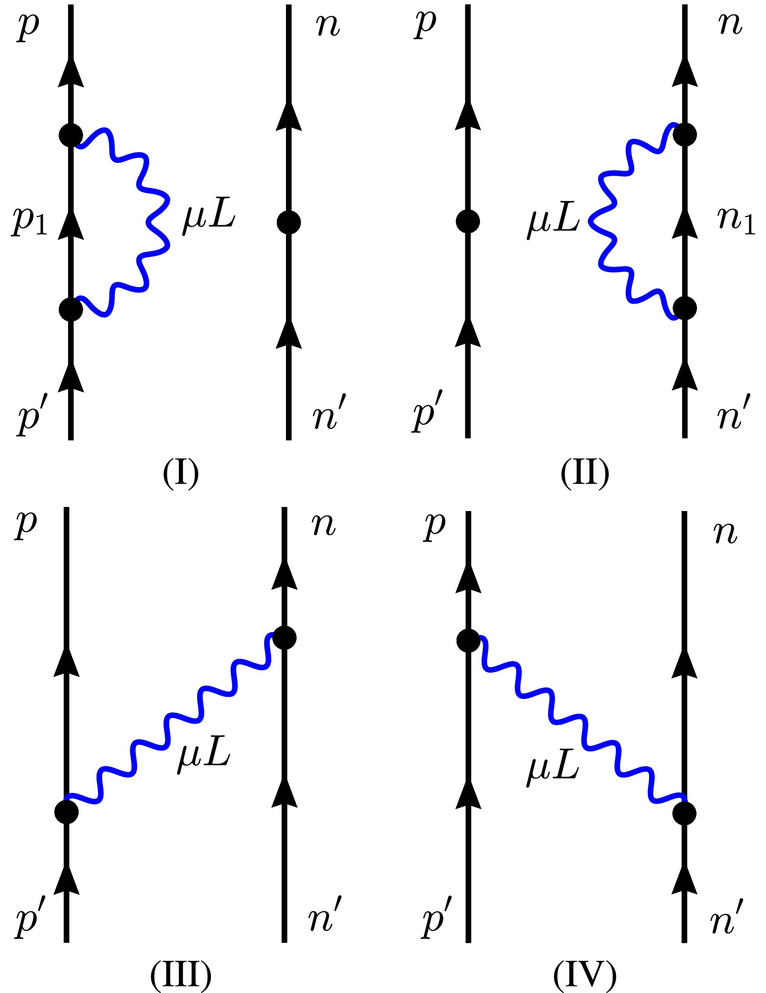

Figure 1.  (color online) Quasiparticle-phonon coupling diagrams contributing to the spreading term $ W^{\downarrow J}_{pn,p'n'} $. Solid arrows denote proton or neutron quasiparticle propagation, wavy lines denote a non-charge-exchange QRPA phonon $ \mu L $, and filled circles denote the coupling vertex $ \gamma^{\mu L} $. In (I) and (II), the neutron and proton are spectators, respectively. In (III) and (IV), the phonon connects the proton and neutron lines in the two possible orientations.

with

The quantities $ E_i $ and $ \Omega_{\mu L} $ represent the quasiparticle and non-charge-exchange QRPA phonon energies, respectively. The reduced quasiparticle-phonon vertex $ \gamma^{\mu L}_{ab} $ is

where $ \mathcal{N}_{ab}^{L} = \sqrt{1 + \delta_{ab}(-1)^L} / (1 + \delta_{ab}) $ is the coupled-pair normalization factor, and $ \hat{L} = \sqrt{2L + 1} $. The terms $ X^{\mu L}_{ab} $ and $ Y^{\mu L}_{ab} $ represent the forward and backward amplitudes of the non-charge-exchange QRPA phonon $ |\mu L \rangle $. The effective interaction involved in this vertex is

Here, u and v represent the BCS occupation amplitudes. The matrix elements for the particle-hole and particle-particle residual interactions, denoted as $ V^{{\rm ph},L} $ and $ V^{{\rm pp},L} $ respectively, are provided in detail in Appendix A.

At each scanning energy ω, Eq. (22) gives the QPVC response to a one-body external field $ \hat O $. The associated strength function is

Here, Δ represents the smearing parameter. For the GT strength distributions, we set $ \Delta = 1 $ MeV to simulate the experimental resolution, while $ \Delta = 0.2 $ MeV is employed in the β-decay calculations. Since the QPVC Hamiltonian is complex, the numerator is a complex square rather than an absolute square. The term $ \mathcal{M}_k $ is derived from Eq. (21), which provides

where $ M_{\nu J} $ is the pnQRPA transition amplitude.

The operators for GT$ ^\pm $ excitations take the form [1, 4, 55]

where A is the nuclear mass number, $ \sigma_{M} $ is the spherical component of the Pauli spin operator, and $ \tau_\pm $ is the isospin raising or lowering operator.

The quasiparticle energies in the QPVC equation include the neutron and proton chemical potentials. Consequently, the excitation energy relative to the parent ground state for the GT$ ^\pm $ channels is

where the upper (lower) sign applies to GT$ ^+ $ (GT$ ^- $). In the limit of vanishing pairing, this shift recovers the corresponding PVC excitation energy and defines the energy E used below.

With the PCF-PK1 density functional, pnQRPA already provides an accurate description of the GTR centroid energy without any additional phenomenological adjustment ². Therefore, the subtraction method [47, 54] is applied in the calculations of the GTR strength distributions.

The $ \beta^- $ decay half-life in the allowed Gamow-Teller (GT) approximation is determined from the GT$ ^- $ strength within the $ Q_\beta $ decay window [16, 28, 35, 56]:

Here, $ D=6163.4\; \mathrm{s} $, and $ \Delta_{nH}=m_n-m_p-m_e=0.782\; \mathrm{MeV} $ represents the neutron-hydrogen mass difference. The quenched value $ g_A=1.0 $ is adopted. The term $ S_{{\rm GT}^-}^{\beta}(E) $ denotes the GT$ ^- $ strength at the excitation energy E relative to the parent ground state. For a transition occurring at energy E, the maximum total energy of the emitted electron is given by $ E_m=m_e+\Delta_{nH}-E $. The integrated phase-space factor is

Here, $ m_e $, $ p_e $, and $ E_e $ denote the electron rest mass, momentum, and total energy, respectively; $ Z_d=Z+1 $ represents the daughter proton number; and $ F_0 $ is the Fermi function, which includes Coulomb and finite-size corrections [57].

The QPVC strength distribution in Eq. (28) exhibits Lorentzian tails. Within the decay window, as E decreases, the phase-space factor increases approximately as $ (\Delta_{nH}-E)^5 $, which is a more rapid increase than the decrease of the Lorentzian tail. Consequently, even a minor Lorentzian tail can significantly contribute to the decay rate due to the substantial phase-space factor, ultimately leading to a divergence as $ E \rightarrow -\infty $. To prevent this divergence, we substitute the Lorentzian tail of the strength distribution with a Gaussian form, which decays more rapidly than the phase-space factor increases.

We begin by expressing $ \mathcal M_k^2(\omega)=\mathcal R_k(\omega)+\mathrm{i}\mathcal I_k(\omega) $, where $ \mathcal R_k $ and $ \mathcal I_k $ are the real and imaginary components of the complex squared transition amplitude, respectively. With $ x_k=\omega-\Omega_k(\omega) $ and $ a_k=\Gamma_k(\omega)/2+\Delta $, Eq. (28) becomes

The first term has the standard Lorentzian form, which can be directly substituted with a Gaussian form.

with $ \sigma_{1k} = [\Gamma_k(\omega) + 2\Delta] / (2\sqrt{2\ln2}) $. The second term is multiplied by a Gaussian damping factor as follows:

with $ \sigma_{2k} = \Gamma_k(\omega) + 2\Delta $. The total modified strength is

We have confirmed that the modified and original strength distributions exhibit nearly identical peak positions and resonance structures, differing mainly in their far tails. Consequently, the Gaussian-modified GT$ ^- $ strength is employed in the calculation of β-decay half-lives. Notably, the subtraction method is not applied in the QPVC calculation for β-decay half-lives.

The localized RHFB ground-state equations are solved in a harmonic-oscillator basis with an oscillator frequency of $ \hbar\omega_0=70A^{-1/3} $ MeV, including single-particle states with total angular momentum $ j\leq j_{\max}=21/2 $.

In the QRPA calculations, the truncation for two-quasiparticle configurations is controlled by the canonical single-particle energy cutoff $ E_{\rm sp} $ and the occupation-amplitude threshold $ (uv)_{\min}= u_a v_b $, where u and v are the BCS occupation amplitudes for these two quasiparticles. In the QPVC calculations, the pnQRPA states are used as the basis, and an additional cutoff $ B_{\min} $ is applied to this basis. This cutoff represents the minimum non-energy-weighted sum-rule (NEWSR) fraction carried by the pnQRPA states, enhancing calculation efficiency. The selection of phonons entering the doorway state of QPVC calculations is specified by the maximum phonon energy $ E_{\max} $, the maximum total angular momentum $ L_{\max} $ of the phonons, and the collectivity threshold $ v_{\min} $. The threshold $ v_{\min} $ sets the minimum collectivity of the retained phonons, as discussed in detail below.

Using $ ^{74} $Ni as an example, we examine the numerical convergence of the GT$ ^- $ strength distribution calculated by the pnQPVC model using the PCF-PK1 interaction with respect to these parameters in Figs. 2 and 3.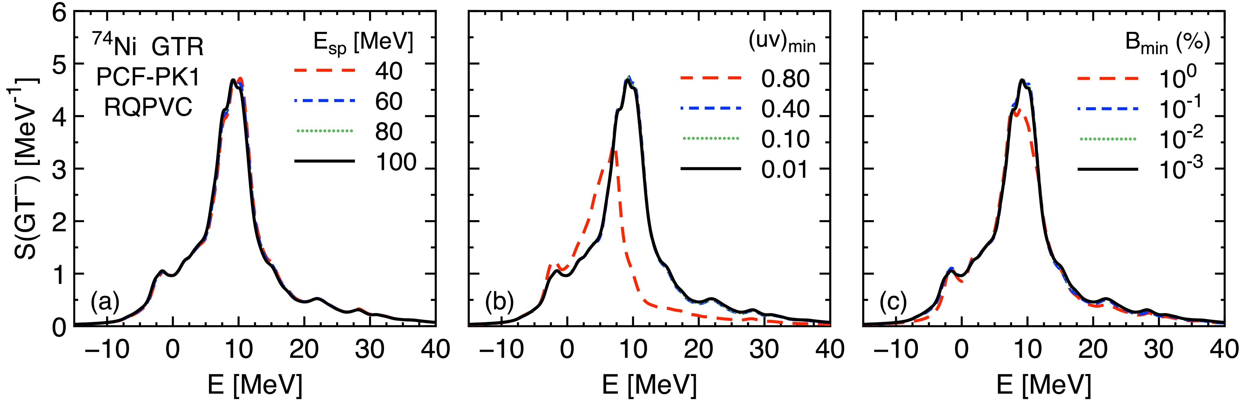

Figure 2.  (color online) Numerical convergence of the GT$ ^- $ strength distribution in $ ^{74} $Ni calculated using the pnQPVC model with the PCF-PK1 interaction. The variables under consideration are: (a) the single-particle energy cutoff $ E_{\rm sp} $, (b) the minimum product of BCS occupation amplitudes $ (uv)_{\min} $, and (c) the minimum NEWSR percentage $ B_{\min} $ carried by a charge-exchange pnQRPA state retained in the pnQPVC basis. In each panel, the other two cutoffs are held constant at their adopted values. The black solid curves represent the final selections: $ E_{\rm sp}=100 $ MeV, $ (uv)_{\min}=0.01 $, and $ B_{\min}=10^{-3}\% $.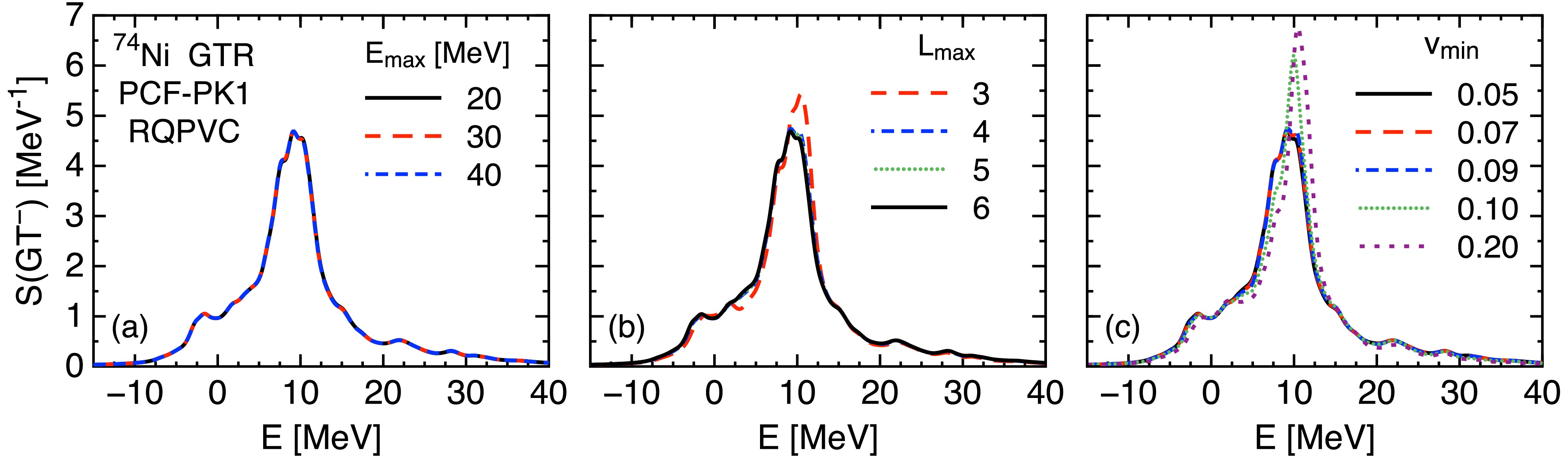

Figure 3.  (color online) The same as Fig. 2, but for the convergence check of phonon space. Panels (a), (b), and (c) illustrate variations in the maximum phonon energy $ E_{\max} $, the maximum total angular momentum $ L_{\max} $ of the phonons, and the collectivity cutoff $ v_{\min} $, respectively. The other two parameters are held constant at their adopted values. The black solid curves represent the final choices: $ E_{\max}=20 $ MeV, $ L_{\max}=6 $, and $ v_{\min}=0.05 $.

Figure 2(a) shows that the curve for $ E_{\rm sp}=40 $ MeV differs around the main resonance, whereas the curves for 60, 80, and 100 MeV are nearly indistinguishable over the full energy interval. Figure 2(b) shows a visible deviation for $ (uv)_{\min}=0.80 $, while the curves for $ (uv)_{\min}=0.40 $, 0.10, and 0.01 are nearly indistinguishable throughout the displayed range. For each charge-exchange pnQRPA state, its discrete GT$ ^- $ strength is evaluated as a percentage of the total GT$ ^- $ non-energy-weighted sum. The state is retained for the pnQPVC basis, as shown in Eq. (21), only when this percentage exceeds $ B_{\min} $. The curve for $ B_{\min}=1\% $ differs around the main resonance, whereas the curves for $ 10^{-1}\% $, $ 10^{-2}\% $, and $ 10^{-3}\% $ are nearly indistinguishable over the displayed range. Consequently, we adopt $ E_{\rm sp}=100 $ MeV, $ (uv)_{\min}=0.01 $, and $ B_{\min}=10^{-3}\% $ in the subsequent calculations, as shown by the black solid curves in Fig. 2.

We next examine the convergence of GT$ ^- $ distributions in Fig. 3 with respect to the cutoff parameters for the phonon space. This space retains only natural-parity phonons, $ \pi=(-1)^L $. Unnatural-parity phonons generally lie at higher excitation energies and are therefore expected to contribute less to the spreading term $ W^\downarrow(\omega) $. The cutoff $ E_{\max} $ limits the energies $ \Omega_{\mu L} $ of the non-charge-exchange phonons, whereas $ L_{\max} $ limits their total angular momenta. The threshold $ v_{\min} $ selects phonons according to their collectivity. Following Ref. [58], we take $ |v_{\mu L}| $ as a measure of collectivity. The selection criterion is

Thus, only phonons with a dimensionless interaction strength $ |v_{\mu L}| $ that exceeds the cutoff $ v_{\min} $ are retained. Here, $ \langle V\rangle_{\mu L} $ represents the expectation value of the residual interaction V in the QRPA phonon state $ |\mu L\rangle $:

$ \Omega_{\mu L} $ is the phonon energy, and $ \langle\Omega^{(0)}_{\mu L}\rangle $ is defined as

where

with

Here, $ h_{ac} $ and $ \Delta_{a\bar c} $ represent the single-particle Hamiltonian and pairing-field matrix elements in the canonical basis, respectively, where $ \bar c $ denotes the time-reversed partner of c.

By incorporating QRPA phonons with $ |v_{\mu L}| \gt v_{\rm min} $, we ensure the inclusion of sufficiently collective phonons to minimize violations of the Pauli principle and mitigate the issue of double counting associated with second-order contributions [58].

Figure 3(a) illustrates a weak dependence on $ E_{\max}=20 $–40 MeV. In Fig. 3(b), the curve for $ L_{\max}=3 $ shows a deviation around the main resonance, whereas the curves for $ L_{\max}=4 $–6 are nearly indistinguishable across the displayed energy range. Figure 3(c) demonstrates that the response remains stable for $ v_{\min}=0.05 $–0.09. Consequently, we adopt $ E_{\max}=20 $ MeV, $ L_{\max}=6 $, and $ v_{\min}=0.05 $ for the subsequent calculations.

With the verified numerical setup, we employ the pnQRPA plus pnQPVC theory to investigate the GT$ ^- $ strength distributions in $ ^{116-134} $Sn, focusing on the effects of QPVC correlations and the roles of the tT and tPV coupling channels. Additionally, we investigate the $ \beta^- $ decay half-lives in neutron-rich Ni and Sn nuclei, as well as in the $ N=50 $ and $ N=82 $ isotones.

Figure 4 compares the QRPA and QPVC GT$ ^- $ strength distributions in even-even $ ^{116-134} $Sn with the available experimental data. In both calculations, the overall GT$ ^- $ strength increases, and the centroid energy shifts downward with the neutron number increasing.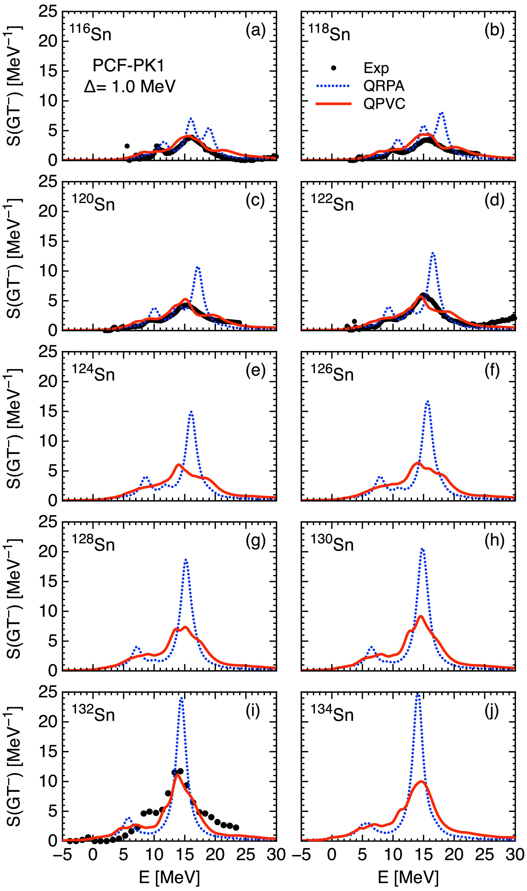

Figure 4.  (color online) GT⁻ strength distributions with respect to the parent nucleus in even-even $ ^{116-134} $Sn are calculated using the QRPA (blue dotted line) and QPVC (red solid line) models, respectively, with the interaction PCF-PK1. Available experimental data (black symbols) are provided for comparison. For $ ^{116,122} $Sn [59] and $ ^{132} $Sn [60], the experimental strengths shown are divided by $ q_{\rm GT}^2 $, where $ q_{\rm GT}=0.75 $. For $ ^{118,120} $Sn, the zero-degree IAS-subtracted cross-sections are converted to equivalent GT strength functions using the formula $ S_{\rm GT}(E)=[d^2\sigma/(d\Omega\,dE)]/[\hat{\sigma}_{\rm GT}F(q,\omega_{\rm tr})] $. Here, $ d^2\sigma/(d\Omega\,dE) $ represents the measured double-differential cross section, $ \hat{\sigma}_{\rm GT} $ is the GT unit cross section, and $ F(q,\omega_{\rm tr}) $ is the kinematic correction at momentum transfer q and reaction energy transfer $ \omega_{\rm tr} $. For $ ^{118} $Sn ($ ^{120} $Sn), $ \hat{\sigma}_{\rm GT}=2.88(24) $ [$ 2.78(16) $] mb/sr and $ F(q,\omega_{\rm tr})=1.04 $ (1.03) are adopted from Ref. [61].

The QRPA strength distribution comprises a low-energy component and a high-energy GTR. As the neutron number approaches $ N=82 $, the high-energy GTR strength evolves from several separated peaks into a single dominant peak.

The low-energy components of these tin isotopes receive contributions from the $ \nu 2d_{5/2}\rightarrow \pi 2d_{3/2} $ spin-flip transition and several non-spin-flip transitions. Beyond $ N=82 $, the occupation of the neutron $ 2f_{7/2} $ orbit introduces a significant $ \nu 2f_{7/2}\rightarrow \pi 2f_{5/2} $ spin-flip contribution in $ ^{134} $Sn. The high-energy GTR is dominated by the $ \nu 1g_{9/2}\rightarrow \pi 1g_{7/2} $ and $ \nu 1h_{11/2}\rightarrow \pi 1h_{9/2} $ transitions. As the neutron number increases toward $ N=82 $, the neutron $ 1h_{11/2} $ orbit becomes progressively filled, enhancing the h-shell transition. The corresponding unperturbed two-quasiparticle energy approaches that of the g-shell transition. Consequently, the residual spin-isospin interaction enhances the mixing of these configurations, concentrating the GTR strength into a single dominant peak from $ N=74 $.

Comparison with experimental data reveals two systematic limitations of QRPA. First, QRPA produces insufficient spreading. In $ ^{116,118} $Sn, it predicts separated GTR peaks, whereas experiments show a single broad resonance. In $ ^{120,122,132} $Sn, the QRPA peaks are too narrow and thus overly strong. Second, the dominant QRPA peaks in $ ^{118-122} $Sn are at higher energies than the measured resonances. Thus, while QRPA captures the evolution of the GTR peak structure with neutron number, it underestimates the spreading and slightly overestimates the resonance energies in the lighter isotopes.

Incorporating the QPVC effect produces a spreading width that significantly broadens the QRPA strength. For $ ^{116-122} $Sn, QPVC merges the separated GTR peaks into a single broad resonance and aligns their energies more closely with experimental data. After $ N=74 $, QPVC reduces the narrow, overly strong QRPA peak, yielding a strength distribution in good agreement with experiment in $ ^{132} $Sn.

Beyond changes in peak positions and widths, the experimental GT strengths are generally lower than the theoretical results. We quantify this difference by integrating the GT$ ^- $ strength within the experimental energy windows and comparing it with the Ikeda sum-rule value $ 3(N-Z) $. For $ ^{116,122,132} $Sn, the experimental fractions are $ (38\pm 7)\% $, $ (48\pm 6)\% $, and $ (56\pm 5 (\rm{stat})_{-10}^{+11}(\rm{syst}))\% $, respectively [59, 60]. This reduction of the measured GT strength relative to the Ikeda sum-rule value is the well-known GT quenching problem. The corresponding pnQRPA fractions are $ 93.0\% $, $ 90.7\% $, and $ 88.3\% $, while pnQPVC gives $ 88.4\% $, $ 85.6\% $, and $ 82.9\% $. Thus, QPVC correlations account for only part of the observed quenching. To compare with experiment, experimental strengths of these nuclei in Fig. 4 are divided by the commonly adopted phenomenological factor $ q_{\rm GT}^{2} $, with $ q_{\rm GT}=0.75 $ [62]. SSRPA studies of GT strength in $ ^{48} $Ca, $ ^{78} $Ni, $ ^{90} $Zr, and $ ^{132} $Sn found that 2p-2h correlations shift substantial strength to higher energies, improving the description of the observed quenching without an additional phenomenological factor [37, 38, 63]. The weaker reduction in QPVC may reflect its restricted space of collective phonons, whereas SSRPA treats a broader set of 2p-2h configurations.

For $ ^{118,120} $Sn, only the double differential cross sections are provided in Ref. [61]. To compare with our calculated results, we extract the GT strength using a simplified procedure: dividing the zero-degree IAS-subtracted cross sections by the GT unit cross section and a constant kinematic correction. The corresponding integrated experimental strengths amount to $ 58.7\% $ and $ 66.1\% $ of the Ikeda sum-rule value, compared with $ 88.1\% $ and $ 88.0\% $ from pnQRPA as well as $ 79.1\% $ and $ 79.3\% $ from pnQPVC, respectively. The QPVC effect accounts for about $ 10\% $ of the quenching, leaving only differences of $ 20.4\% $ and $ 13.2\% $ of $ 3(N-Z) $ from the extracted strengths for $ ^{118} $Sn and $ ^{120} $Sn, respectively. Therefore, we do not introduce any additional phenomenological quenching factor for the two spectra shown in Fig. 4, and the resulting GT strength distribution still agrees well with the experimental data.

Taking $ ^{122} $Sn as an example, Fig. 5 examines the effects of the tT and tPV channels on the GT$ ^- $ strength distribution at the QRPA and QPVC levels. In panel (a), the full charge-exchange QRPA residual interaction shifts the unperturbed strength to higher energies and concentrates it into a collective peak near 17 MeV. Omitting either tT (blue dashed line) or tPV (red dash-dotted line) shifts the strength to lower energies and redistributes it among several peaks. The comparable changes show that the two channels provide similar repulsive contributions. When both channels are omitted, the strength distribution (green dashed line) nearly recovers the unperturbed result, showing that their combined repulsive contribution produces the collective GTR.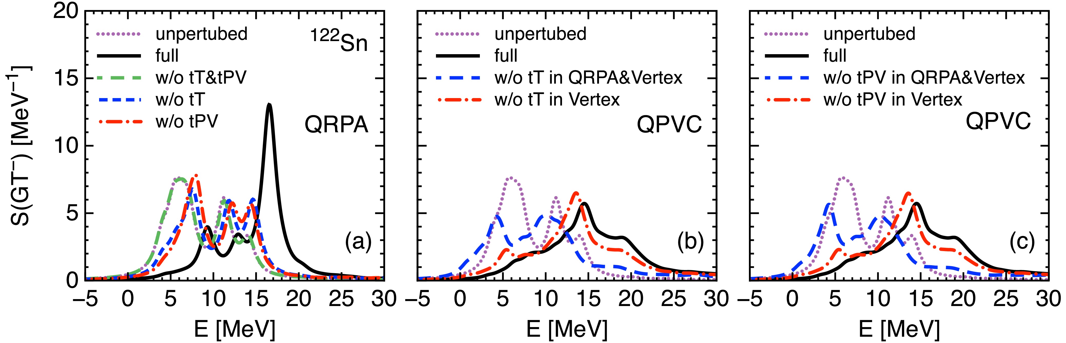

Figure 5.  (color online) Effects of the isovector-tensor (tT) and isovector-pseudovector (tPV) coupling channels on the GT$ ^- $ strength distribution in $ ^{122} $Sn. Panel (a) compares the unperturbed response with the full pnQRPA result and pnQRPA calculations where the tT, tPV, or both channels are omitted from the pnQRPA residual interaction. Panel (b) contrasts the unperturbed response with the full pnQPVC result, the pnQPVC calculation where the tT channel is omitted only in the QPVC vertex, and the pnQPVC calculation where the tT channel is omitted in both the pnQRPA and QPVC vertex. Panel (c) is the same as panel (b) but for the tPV channel. In all QPVC results, non-charge-exchange phonons are calculated by QRPA with the full residual interaction.

Panels (b) and (c) separate the effects of tT and tPV in the charge-exchange QRPA residual interaction from their contributions through the QPVC vertices. Removing tT or tPV only from the QPVC vertices produces little change relative to the full QPVC result, indicating that their contributions through the vertices are small. In contrast, removing the same channel also from the charge-exchange QRPA residual interaction substantially changes the strength distribution, showing that tT and tPV affect the GTR mainly at the QRPA level. When tT or tPV is omitted from both the QRPA residual interaction and the QPVC vertices, QPVC correlations still broaden the QRPA strength and shift it toward lower excitation energies, even slightly below the unperturbed peaks. The remaining broadening and downward energy shifts therefore arise mainly from the other coupling channels in the QPVC vertices.

Having examined the GTR strength distributions, we now focus on the $ \beta^- $-decay half-lives and evaluate the effects of QPVC correlations. The roles of the tT and tPV channels are analyzed separately, using $ ^{134} $Sn as an example.

Figure 6 compares the calculated $ \beta^- $-decay half-lives along the neutron-rich Ni and Sn isotopic chains with experimental data. For both chains, QRPA generally overestimates the measured half-lives, whereas QPVC reduces them. This reduction occurs because QPVC redistributes GT strength toward lower energies, where the decay phase-space factor is larger, thereby shortening the half-lives [35].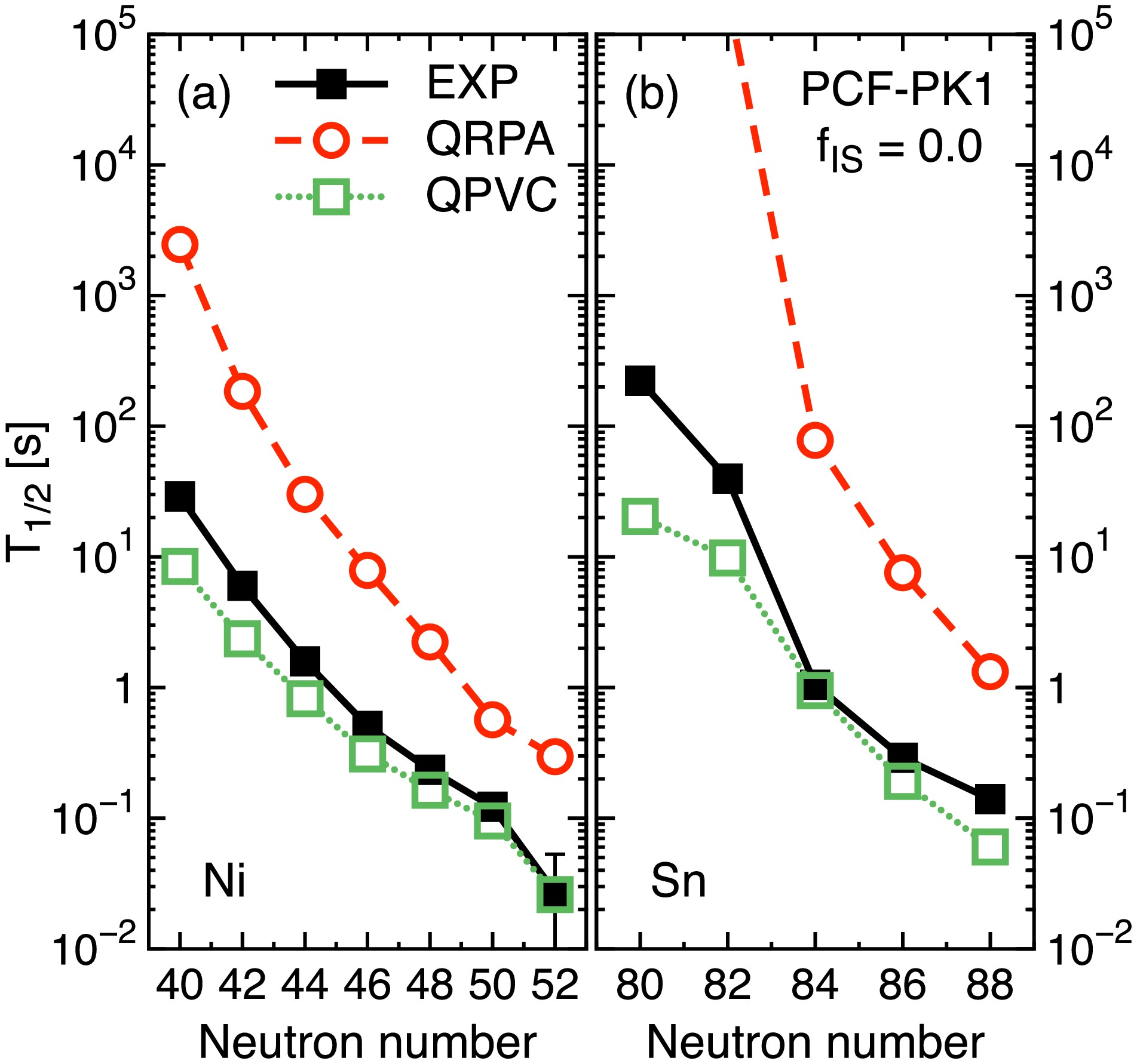

Figure 6.  (color online) $ \beta^- $-decay half-lives along the (a) Ni and (b) Sn isotopic chains are presented. Black solid squares represent experimental values [64, 65]; red dashed lines with open circles and green dotted lines with open squares indicate the QRPA and QPVC results, respectively. All calculations employ PCF-PK1, consider only allowed GT transitions, and set the isoscalar pairing strength to $ f_{\rm IS}=0 $

For the Ni isotopes in Fig. 6(a), QRPA systematically overestimates the measured half-lives and shows only a weak change from $ N=50 $ to 52, failing to capture the rapid experimental decrease across the magic number. This experimental phenomenon is reproduced by QPVC, which lowers the half-lives at $ N=52 $ more substantially than at $ N=50 $.

For the Sn isotopes in Fig. 6(b), the QRPA half-lives at $ N=80 $ and 82 exceed the displayed range. QPVC significantly reduces these half-lives but underestimates the experimental values. From $ N=84 $ to 88, QRPA overestimates the measured half-lives by about one to two orders of magnitude, whereas QPVC brings the predictions closer to the experimental data. QPVC also reproduces the pronounced experimental decrease from $ N=82 $ to 84, although the calculated change is less pronounced because the $ N=82 $ half-life is underestimated.

In Fig. 7(a), both models predict increasing half-lives along the $ N=50 $ isotonic chain with increasing proton number. However, QRPA significantly overestimates the half-lives and the growth trend with proton number. In contrast, QPVC properly reproduces the measured half-life magnitudes and their increasing trends. For the $ N=82 $ chain in Fig. 7(b), the measured half-lives increase sharply at the magic number $ Z=50 $. QRPA greatly overestimates this increasing trend and even predicts $ ^{134} $Te to be stable against $ \beta^- $ decay. QPVC offers a much better description of the abrupt change at the magic number, as well as the overall experimental systematics. For the $ N=50 $ isotonic chain, QPVC also predicts an abrupt change at the magic number $ Z=28 $, which requires confirmation by future experiments.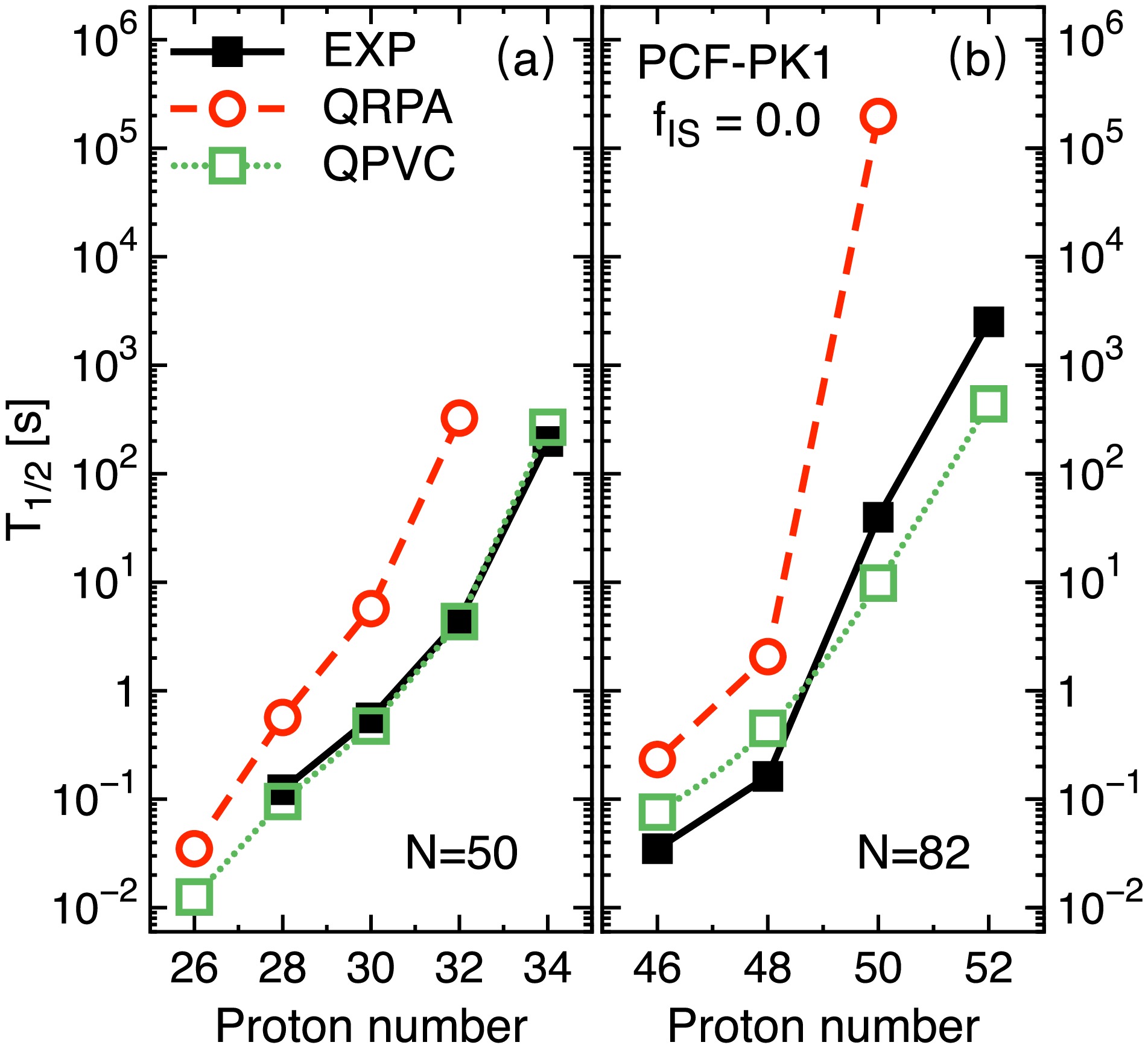

Figure 7.  (color online) Same as Fig. 6, but for the isotonic chains with (a) $ N=50 $ and (b) $ N=82 $.

Taking $ ^{134} $Sn as an example, Fig. 8 examines the roles of the tT and tPV channels in the calculated $ \beta^- $-decay half-life. When both channels are omitted, the QRPA alters the half-life only slightly from the unperturbed result. Successively restoring tPV and then tT increases the half-life to $ 77.943 $ s in the full QRPA calculation. This behavior is consistent with their repulsive effects on the GT strength distribution in Fig. 5(a): both channels shift the GT strength to higher energies, where the phase-space factor is smaller, thereby lengthening the half-life. The tT and tPV channels thus account for most of the QRPA-induced increase in the $ ^{134} $Sn half-life.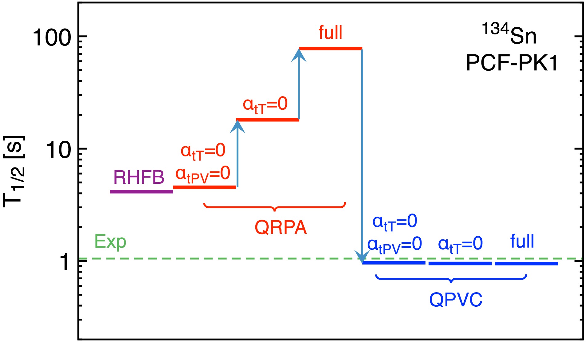

Figure 8.  (color online) Effects of the tT and tPV channels on the calculated $ \beta^- $-decay half-life of $ ^{134} $Sn. The green dashed line represents the experimental value [64]. The purple segment illustrates the unperturbed two-quasiparticle result, whereas the red and blue segments depict the pnQRPA and pnQPVC results, respectively. In the red pnQRPA sequence, $ \alpha_{\rm tT}=0 $ and $ \alpha_{\rm tT}=\alpha_{\rm tPV}=0 $ indicate the exclusion of the specified channels from the pnQRPA residual interaction. In the blue pnQPVC sequence, these labels signify their exclusion solely from the QPVC vertices, while the complete pnQRPA calculation is maintained. The label "full" refers to calculations without any channel exclusion.

At the QPVC level, omitting only tT, or both tT and tPV, from the vertices changes the half-life by less than $ 2\% $, indicating that their contributions through the vertices are minimal. The substantial reduction from the full QRPA result persists and therefore arises mainly from the other coupling channels in the QPVC vertices. This behavior is consistent with the GTR analysis in Figs. 5(b) and (c). The complete QPVC calculation yields $ 0.948 $ s, which is close to the experimental value of $ 1.050 $ s.

We have developed a relativistic proton-neutron quasiparticle random-phase approximation (pnQRPA) plus proton-neutron quasiparticle-vibration coupling (pnQPVC) model for charge-exchange excitations, based on localized RHFB theory with the PCF-PK1 functional. This model incorporates exchange terms localized through the Fierz transformation as well as tensor couplings. The residual interaction of pnQRPA, particularly the tPV channel, is determined fully self-consistently without phenomenological adjustment. Building on the pnQRPA basis, the model incorporates two-quasiparticle-phonon doorway configurations to account for correlations beyond pnQRPA.

Applying the newly developed relativistic pnQPVC model, we find that, compared with pnQRPA, QPVC broadens and redistributes the GT strength in $ ^{116-134} $Sn, improving the calculated GTR widths and strength distributions relative to experimental data. QPVC also substantially reduces the calculated β-decay half-lives, enhancing agreement with experimental trends along the neutron-rich Ni and Sn isotopic chains, as well as the $ N=50 $ and $ N=82 $ isotonic chains. Channel analyses further show that tT and tPV channels affect the GT response and β-decay half-lives mainly through the pnQRPA residual interaction, whereas their contributions through the QPVC vertices are minimal.

In the present calculations, QPVC-induced correlations in the parent ground state are not included. Such correlations admix configurations beyond the quasiparticle-vacuum reference and may shift GT strength to higher energies, thereby lengthening the calculated half-lives, which may be essential for nuclei whose half-lives are underestimated in the present calculations. The present β-decay calculations are also restricted to allowed GT transitions. First-forbidden transitions can become significant near shell closures and generally shorten the half-lives by opening additional decay channels [52]. Consistently including ground-state correlations and first-forbidden transitions may therefore further improve the description of β-decay half-lives presented in this work.

This appendix provides the particle-hole (ph) and particle-particle (pp) residual-interaction matrix elements in Eq. (27), which are utilized in the QPVC vertices for coupling to non-charge-exchange phonons. The ph channel is derived from the second derivative of the energy density functional used for the ground state in Eq. (10), evaluated at the ground-state density $ \rho_0 $,

with the rearrangement term

For a spherical nucleus, coupling the two-body matrix elements of this kernel to the phonon's total angular momentum L results in

Here, $ \alpha=(a,m_\alpha) $, $ C_{j_1m_1 j_2m_2}^{LM} $ denotes a Clebsch-Gordan coefficient, and M is the projection of the total angular momentum L. The quantity $ \mathcal N_{ab}^{L} $ is the normalization factor for the angular-momentum-coupled pair, as defined following Eq. (26).

The complete ph matrix element is given by

where $ V_{ab,cd}^{{\rm C},L} $ and $ V_{ab,cd}^{{\rm der},L} $ represent the Coulomb and scalar-derivative contributions, respectively. The scalar-derivative contribution is

The Coulomb matrix element is decomposed as: $ V_{ab,cd}^{{\rm C},L}=V_{ab,cd}^{{\rm C},0,L} +V_{ab,cd}^{{\rm C},{\rm s},L} $. The expressions below represent its temporal and spatial components, respectively:

Here, $ j_\lambda(kr) $ denotes a spherical Bessel function of the first kind, with $ \lambda = L $ or $ \ell $.

The matrix elements $ V_{ab,cd}^{\chi,L} $ represent the scalar (S), isovector-scalar (tS), vector (V), isovector-vector (tV), tensor (T), isovector-tensor (tT), pseudoscalar (PS), isovector-pseudoscalar (tPS), pseudovector (PV), and isovector-pseudovector (tPV) contributions. In contrast, $ V_{ab,cd}^{{\rm R},\chi,L} $ denote the corresponding rearrangement terms, where $ \chi = {\rm S, tS, V, tV, T, tT, PS, tPS, PV, tPV} $. In the ground states of even-even nuclei, parity and time-reversal invariance result in the PS, tPS, PV, and tPV densities vanishing, thus eliminating any rearrangement contributions from these channels.

The V, tV, T, tT, PV, and tPV contributions can be decomposed into temporal and spatial components,

The contributions from the S, tS, PS, and tPS channels, along with the temporal components of the V, tV, T, tT, PV, and tPV channels, are expressed as follows:

In the matrix elements above, $ G_x(r) $ and $ F_x(r) $ represent the radial wave functions of the large and small components of the canonical Dirac state x, respectively. Here, $ q_x=1 $ for a neutron and $ q_x=-1 $ for a proton, while $ Q_x=(1-q_x)/2 $. The operator $ \mathscr T_{L\ell M}(\hat{\boldsymbol r}) $ appearing in the aforementioned matrix elements is defined by

The reduced angular matrix elements read

A prime on a state label denotes the component with $ l'_a = 2j_a - l_a $. The isovector factor in these expressions is given by

The spatial components of the V, tV, T, tT, PV, and tPV channels are expressed by the following equations:

Density dependence generates the following non-zero rearrangement contributions:

The rearrangement contributions involve the ground-state densities:

For the non-charge-exchange excitations, the separable pp interaction in Eq. (8) acts between proton-proton and neutron-neutron pairs in the $ (S,T)=(0,1) $ channel. Its angular-momentum-coupled matrix element takes the form

In a spherical harmonic-oscillator basis, separable pp interaction gives

with

where N and n represent the radial harmonic-oscillator quantum numbers for the center-of-mass and relative coordinates, respectively. Here, $ R_{n0}(r,b_0) $ denotes the radial harmonic-oscillator wave function with oscillator length $ b_0 $, and $ M_{n_al_an_bl_b}^{NLn0} $ is a Talmi-Moshinsky bracket that satisfies

Transforming the oscillator-basis matrix elements to the canonical basis yields the pp matrix element that enters the effective interaction in Eq. (27),

Here, $ D_{ia}=\langle i|a\rangle $ represents the expansion coefficient of the canonical state a in the oscillator basis state i.