Quasinormal modes of massless scalar and electromagnetic perturbations for Euler–Heisenberg black holes surrounded by perfect fluid dark matter

The detection of gravitational waves from compact binary mergers by the LIGO and Virgo Collaborations [1, 2] has opened a new observational window into the strong-field regime of gravity. In particular, the ringdown phase of a perturbed black hole is governed by quasinormal modes (QNMs), which characterize the damped oscillations of spacetime under external perturbations [3−5]. Since the quasinormal spectrum depends on the parameters of the black hole and the underlying gravitational theory, QNMs provide powerful probes of black hole physics and possible deviations from general relativity [6, 7]. In recent years, quasinormal spectra have been extensively investigated for charged black holes in higher-dimensional theories [8], regular and scale-dependent black holes [9−11], black holes in modified gravity [12], and AdS black holes in critical gravity [13]. The pursuit of non-singular spacetimes is also a central theme in broader quantum gravity frameworks, where non-singular cosmological evolutions have been explored in Loop Quantum Cosmology-inspired M-theory models [14].

Meanwhile, dark matter remains one of the most important open problems in modern cosmology and astrophysics. Observations of galactic rotation curves [15], galaxy cluster dynamics [16], and cosmic microwave background measurements [17] provide compelling evidence for its existence. Among the various phenomenological models, perfect fluid dark matter (PFDM) offers an effective framework for describing dark matter environments around black holes [18, 19, 37, 38]. In this model, the surrounding dark matter distribution introduces logarithmic corrections to the spacetime geometry, thereby modifying particle motion, effective potentials, and wave propagation near black holes. Notably, the quasinormal modes and absorption cross sections of a Bardeen black hole surrounded by PFDM were recently studied in four dimensions [20].

In parallel, nonlinear electrodynamics plays an important role in regimes with strong electromagnetic fields. The Euler–Heisenberg (EH) effective action, derived from one-loop quantum electrodynamics [21, 22], describes vacuum polarization effects and naturally extends classical Maxwell theory. Black holes in nonlinear electrodynamics exhibit rich physical properties, including modified horizon structures, thermodynamics, optical behavior, and perturbation spectra [23, 24]. In particular, non-singular black hole solutions constructed via gravitational decoupling have been explored for their thermodynamic properties [25], and the quasinormal modes of Bardeen black holes with a cloud of strings have been systematically analyzed [11]. Recently, Euler–Heisenberg black holes surrounded by PFDM have attracted considerable attention [26, 27]. Such spacetimes incorporate both one-loop QED corrections characterized by the EH parameter a and logarithmic dark matter corrections governed by the PFDM parameter λ, leading to rich phenomenological structures.

Recently, Belchior et al. [49] investigated the greybody factors and absorption cross sections of spin-$ 0 $, $ 1 $, and $ 1/2 $ fields propagating in Euler–Heisenberg black holes surrounded by PFDM. Using the Boonserm–Visser rigorous bound method, they showed that both the EH parameter and the PFDM parameter significantly modify the effective potential barrier and transmission probability. Meanwhile, greybody factors and their rigorous bounds have also been studied for quantum-corrected black holes [28] and regular scale-dependent black holes [29], while the greybody factors of four-dimensional AdS black holes in critical gravity were investigated together with their thermodynamic properties [13]. In addition, optical properties and shadow structures of black holes in dark matter environments have been extensively studied in recent years [30, 31]. The intrinsic connections between the shadow radius and quasinormal modes in the eikonal limit have been established for specific black hole spacetimes [32], and the correspondence between gravitational-wave signals and black hole imaging has been explored for modified black holes [33].

While these recent studies [49, 50] provide valuable insights into the scattering and optical properties of Euler–Heisenberg black holes surrounded by PFDM, they are subject to inherent methodological limitations. Specifically, Ref. [49] employs the Boonserm–Visser rigorous lower-bound method, which yields analytical bounds but cannot provide the exact transmission probabilities required for precise absorption cross sections. Ref. [50] relies on the eikonal quasinormal-mode correspondence, which is valid only in the large-angular-momentum limit ($ l \to \infty $) and fails to capture the greybody behavior at low multipoles, which is crucial for astrophysical Hawking radiation spectra. Moreover, neither work computes the full quasinormal-mode spectrum in conjunction with greybody factors within a single self-consistent framework beyond the eikonal limit. In addition, asymptotically flat black holes remain of particular astrophysical relevance, since realistic black holes such as M87^* [30] and Sagittarius A^* [31] can be effectively described within asymptotically flat backgrounds.

Motivated by these considerations, in this work we systematically investigate the quasinormal modes and greybody factors of massless scalar and electromagnetic perturbations around asymptotically flat Euler–Heisenberg black holes surrounded by PFDM. The quasinormal frequencies are computed using the asymptotic iteration method (AIM) [34] together with the sixth-order WKB approximation [35] for comparison and consistency checks. We analyze the effects of the black hole charge Q, the Euler–Heisenberg parameter a, and the PFDM parameter λ on the oscillation frequencies and damping rates. Our results reveal characteristic signatures of nonlinear electrodynamics and dark matter effects in black hole ringdown signals, providing potential theoretical predictions for future gravitational-wave observations.

This paper is organized as follows. In Sec. II, we present the Euler–Heisenberg black hole spacetime in perfect fluid dark matter and derive the perturbation equations for scalar and electromagnetic fields, along with the corresponding effective potentials. In Sec. III, we calculate the fundamental quasinormal frequencies using the asymptotic iteration method and the sixth-order WKB approximation, and analyze their dependence on the charge Q, nonlinear electrodynamics parameter a, dark matter parameter λ, and angular momentum l. In Sec. IV, we evaluate the greybody factors using the WKB method. Finally, we conclude and discuss the observational implications in Sec. V. The numerical methods are detailed in the Appendices.

The spacetime geometry of an EH black hole surrounded by PFDM, originally constructed in Refs. [26, 27], is described by the following static, spherically symmetric line element

where the metric function $ f(r) $ is given by [26, 27]

Here, M and Q denote the black hole mass and magnetic charge, respectively, whereas the parameter a characterizes the nonlinear corrections associated with Euler–Heisenberg electrodynamics [21−23]. The PFDM contribution is encoded by the parameter λ, which measures the intensity of the surrounding dark matter distribution [18, 19].

Several well-known black hole solutions can be recovered for particular parameter limits:

● In the limit $ \lambda \to 0 $, the solution reduces to the standard Euler–Heisenberg (EH) black hole spacetime [26, 27].

● For $ Q \to 0 $, the spacetime reduces to a Schwarzschild black hole surrounded by PFDM [18, 19].

● In the limits $ Q \to 0 $ and $ \lambda \to 0 $, the metric further reduces to the Schwarzschild black hole solution [39].

● In the simultaneous limits $ a \to 0 $ and $ \lambda \to 0 $, the metric reduces to the Reissner–Nordström black hole solution [40, 41].

When the scalar field is treated as a test perturbation propagating in a fixed black hole background, its dynamics is governed by the massless Klein–Gordon equation.

After substituting the metric (1) into Eq. (3), the scalar field can be decomposed using separation of variables as [42]

where $ Y_{lm}(\theta,\varphi) $ denotes a spherical harmonic function. After separating the angular variables, the radial part of the perturbation equation can be recast in Schrödinger-like form.

where the tortoise coordinate $ r_* $ is defined by

Here, $ \psi_s(r) $ denotes the radial wave function, and ω is the quasinormal frequency. The effective potential $ V_s(r) $ is given by [42]

where l denotes the multipole number of the quasinormal modes. Thus, the effective potential depends on both the black hole spacetime geometry and the multipole number l.

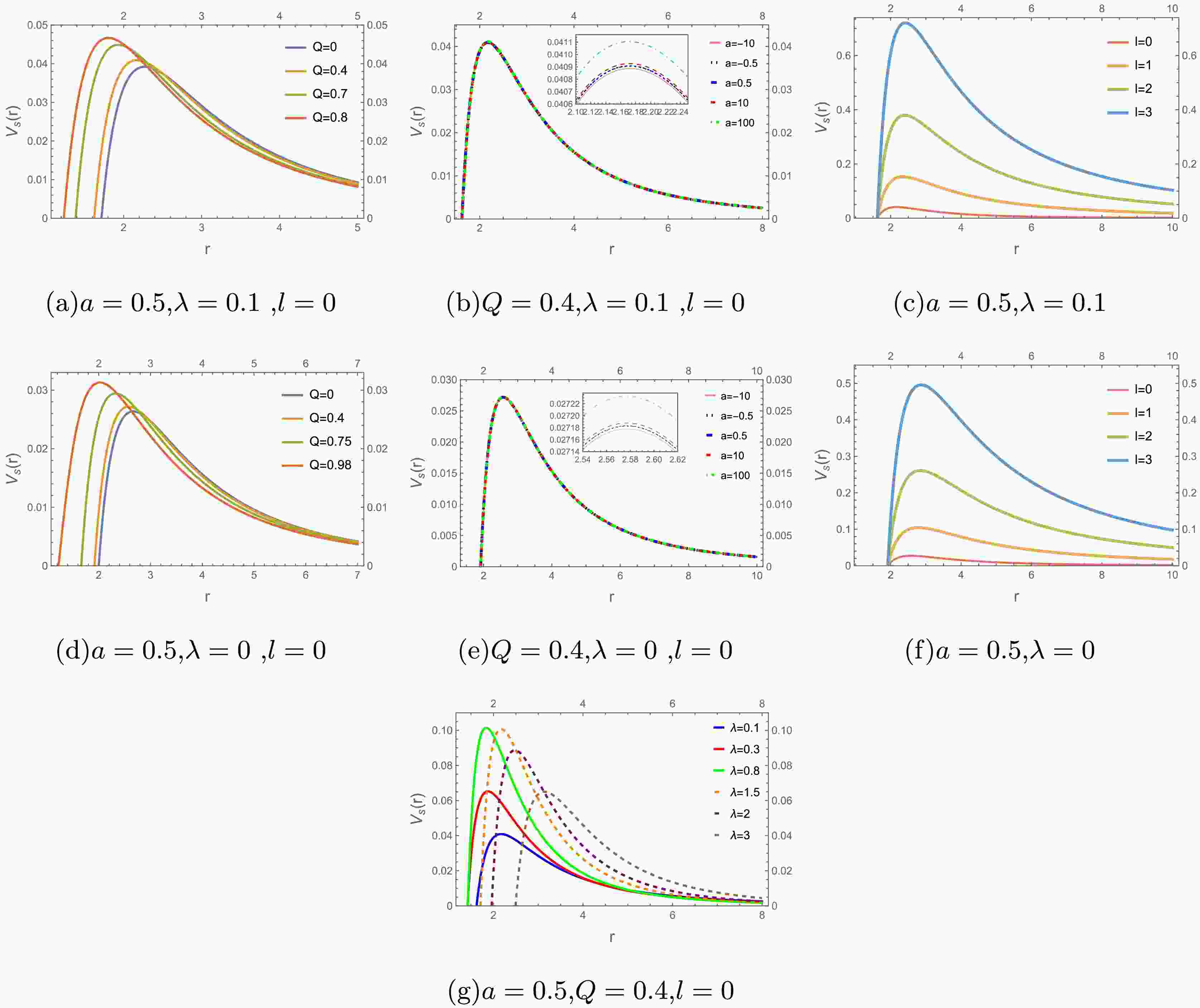
Fig. 1 shows the effective potential $ V_{s}(r) $ for massless scalar perturbations around the Euler–Heisenberg black hole surrounded by perfect fluid dark matter, with $ M=1 $. Figs. 1(a) and 1(d) show that the potential barrier increases monotonically with the black hole charge Q, becoming higher and slightly narrower. The PFDM background ($ \lambda=0.1 $) consistently produces a larger barrier than the vacuum case. Figs. 1(b) and 1(e) indicate that the barrier height increases with the Euler–Heisenberg parameter a, although this effect remains relatively weak and the overall profile changes only slightly. Figs. 1(c) and 1(f) demonstrate that increasing l substantially raises and narrows the barrier, accompanied by a small outward shift in the peak position, confirming the dominant role of the angular momentum term in the scalar effective potential. Fig. 1(g) reveals a nonmonotonic dependence on λ: the barrier becomes higher and narrower at small and intermediate λ, whereas sufficiently large λ leads to a lower and broader barrier. These results indicate that l, Q, and λ primarily govern the scalar effective potential, whereas the nonlinear parameter a introduces only mild corrections near the horizon.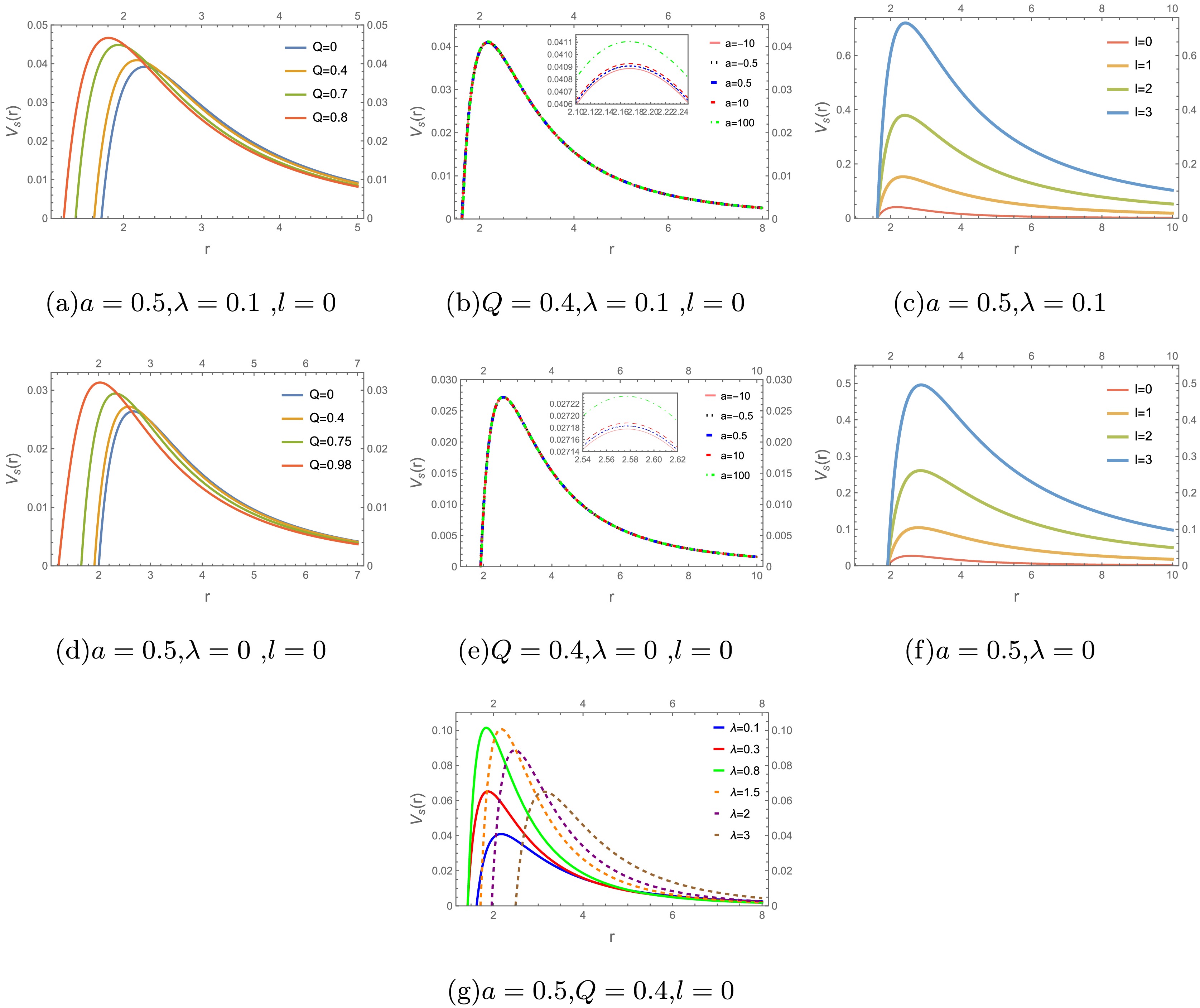

Figure 1.  (color online) The effective potential $ V_s(r) $ for massless scalar-field perturbations of a black hole with $ M=1 $.

Maxwell’s equations govern the dynamics of a massless electromagnetic field propagating in curved spacetime and minimally coupled to the background geometry.

where the electromagnetic field-strength tensor is defined as

where $ A_\mu $ denotes the vector potential of the perturbed electromagnetic field. Using the standard decomposition in spherical symmetry [42, 43], the vector potential can be expressed as

where $ Y_{l,m}(\theta,\varphi) $ are the spherical harmonics, and l and m denote the angular and azimuthal quantum numbers, respectively. The first term in Eq. (10) corresponds to the axial (odd-parity) sector, with parity $ (-1)^{l+1} $, whereas the second term represents the polar (even-parity) sector, with parity $ (-1)^l $.

Upon substituting the above decomposition into Maxwell’s equations (8), both the axial and polar electromagnetic perturbations can be reduced to a unified Schrödinger-like wave equation,

where the effective potential [42, 43] is given by

The master variable $ \Psi_e(r) $ has different forms in the odd- and even-parity sectors:

Fig. 2 displays the effective potential $ V_{e}(r) $ for massless electromagnetic perturbations around the Euler–Heisenberg black hole surrounded by perfect-fluid dark matter with $ M=1 $. Figs. 2(a) and 2(d) show that the potential barrier increases with the black hole charge Q, with the enhancement becoming more pronounced near the extremal regime, as in the scalar case. Figs. 2(b) and 2(e) indicate that the barrier height decreases slightly as the Euler–Heisenberg parameter a increases, although the overall potential profile remains nearly unchanged. This behavior reflects the weak influence of the nonlinear correction on electromagnetic perturbations. Figs. 2(c) and 2(f) demonstrate that increasing l substantially raises and narrows the barrier, with a smoother and more regular variation than that observed for scalar perturbations. Fig. 2(g) reveals a nonmonotonic dependence on λ: the barrier becomes higher and narrower for small λ, whereas sufficiently large λ yields a lower and broader barrier. These results confirm that l, Q, and λ primarily govern the electromagnetic effective potential, whereas the nonlinear parameter a introduces only mild near-horizon corrections.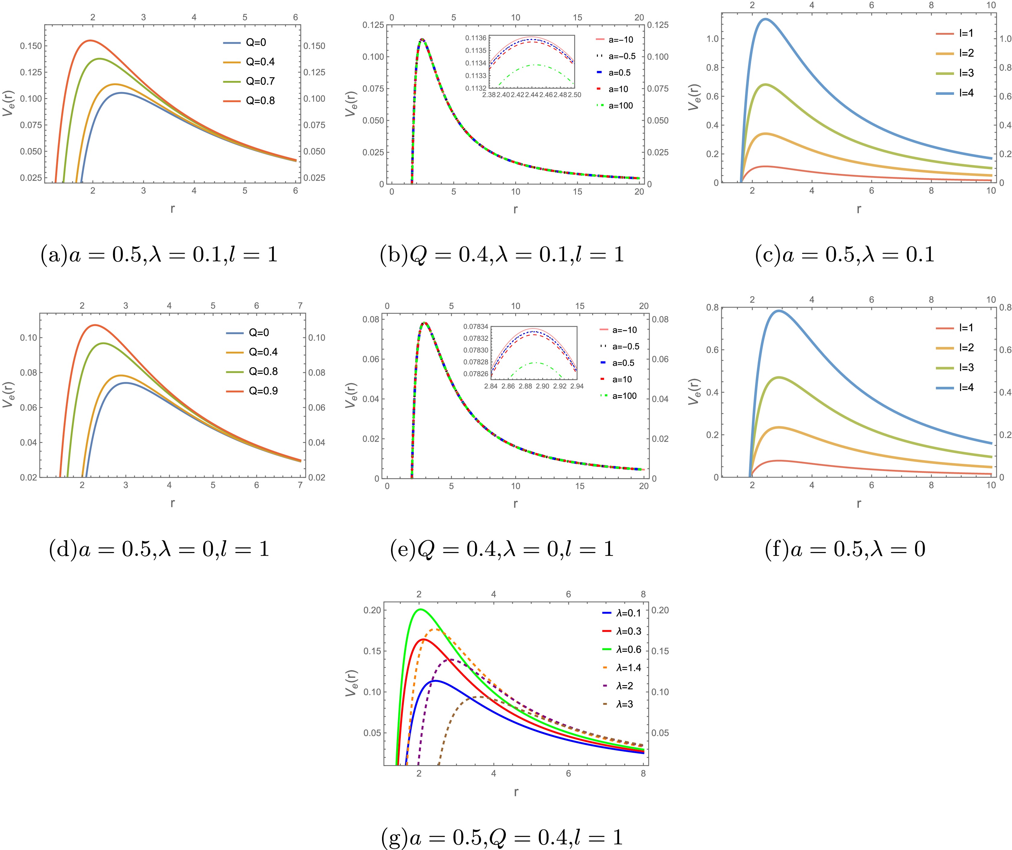

Figure 2.  (color online) The effective potential $ V_e(r) $ for a massless electromagnetic field in the background of a black hole with $ M=1 $.

Having constructed the effective potentials for scalar and electromagnetic perturbations, we proceed to compute the quasinormal frequencies (QNFs) of magnetically charged Euler–Heisenberg black holes surrounded by perfect fluid dark matter. The quasinormal frequencies ω are the characteristic complex oscillation frequencies of the perturbed spacetime, subject to physically motivated boundary conditions [4, 5] imposed on the radial wave function:

which require purely ingoing wave solutions at the event horizon and purely outgoing wave solutions at spatial infinity.

Because the perturbation equations do not admit closed-form analytical solutions, we employ two independent high-precision numerical approaches to determine the fundamental quasinormal frequencies ($ n=0 $), which dominate the black hole ringdown signal in gravitational-wave observations. Specifically, we use the asymptotic iteration method (AIM) [34] and the sixth-order Wentzel–Kramers–Brillouin (WKB) approximation [35]. For completeness, detailed implementations of both methods are summarized in Appendices A and B.

To quantify the consistency between the two sets of results, we define the relative percentage deviation

This provides a reliability check for our computed QNFs.

Our numerical results for the fundamental modes are systematically presented in Tables I and II, and the parametric dependence on the black hole charge Q, nonlinear parameter a, dark matter parameter λ, and angular momentum l is illustrated in Figs. 3–14. Throughout the analysis, we focus on the fundamental mode $ n=0 $, which has the longest damping time and dominates the late-time ringdown waveform. Although the first overtone ($ n=1 $) has been identified in the ringdown analysis of GW150914 [36], higher overtones ($ n\geq 2 $) decay much more rapidly and contribute subdominantly to the observed signal. Extensions to higher overtones will be considered in future work.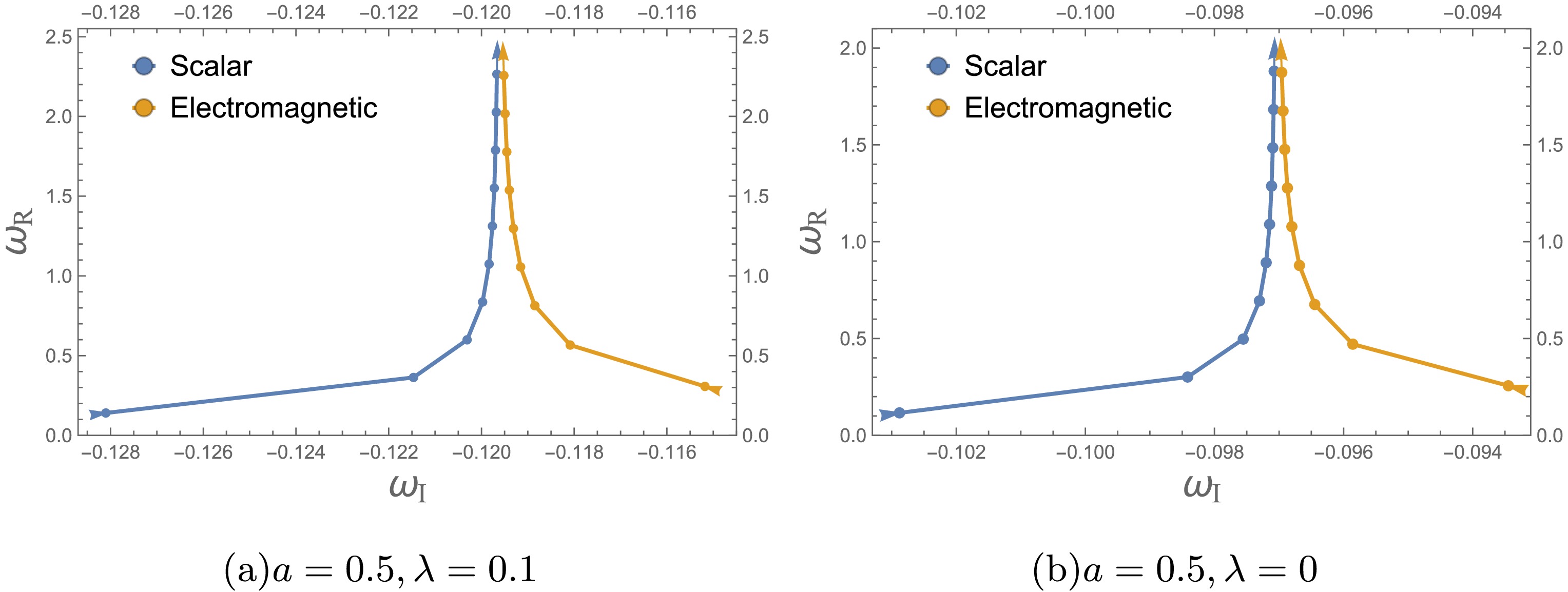

Figure 3.  (color online) Variation of scalar and electromagnetic fundamental QNFs ($ n=0 $) for different values of l, with $ M=1 $ and $ Q=0.4 $. The arrow indicates the direction of increasing angular momentum parameter l. Panels (a) and (b) show the scalar field modes with $ l=0, 1, 2, 3, 4, 5, 6, 7, 8 $ and the electromagnetic field modes with $ l=1, 2, 3, 4, 5, 6, 7, 8 $, respectively.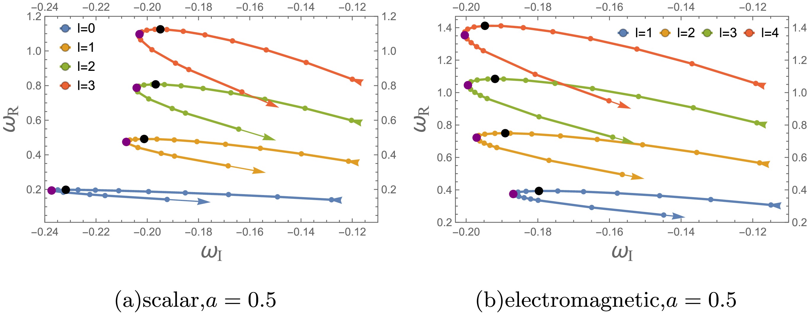

Figure 4.  (color online) Variation of the scalar and electromagnetic fundamental QNFs ($ n=0 $) as functions of λ for $ M=1 $ and $ Q=0.4 $. The arrows in panels (a) and (b) indicate the direction of increasing λ for $ \lambda\in[0.1,3] $. Black dots mark the maxima of $ \omega_{\rm{R}} $, and purple dots mark the minima of $ \omega_{\rm{I}} $ as functions of λ. For scalar QNFs with $ l=0,1,2,3 $, the black dots occur near $ \lambda=0.9,0.8,0.77,0.75 $, respectively, and the purple dots occur near $ \lambda=1.22,1.19,1.17,1.15 $, respectively. For electromagnetic QNFs with $ l=1,2,3,4 $, the black dots occur near $ \lambda=0.7,0.73,0.75,0.8 $, respectively, and the purple dots occur near $ \lambda=1.1,1.13,1.15,1.2 $, respectively.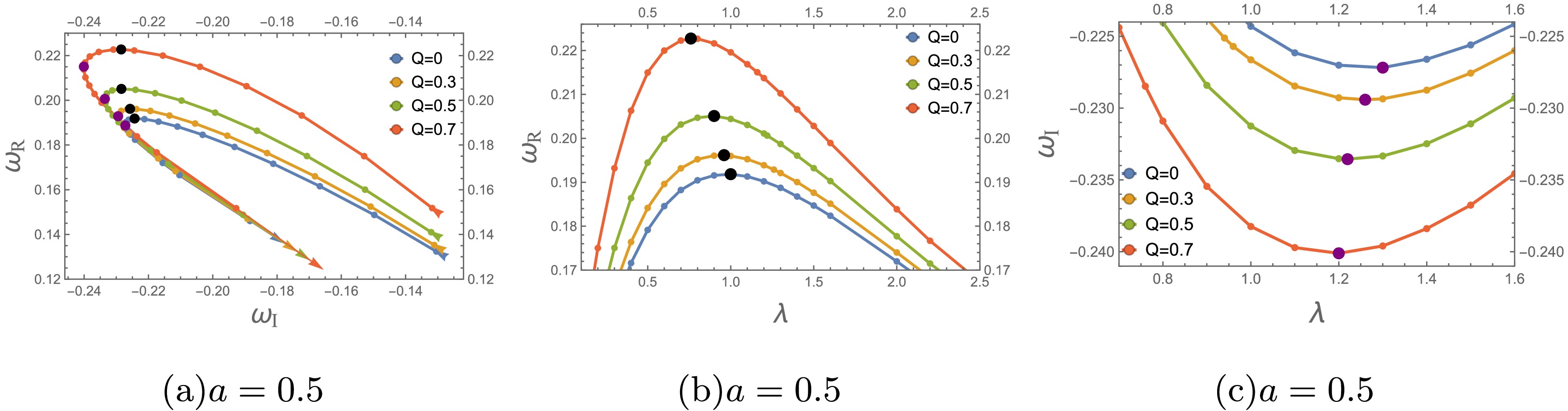

Figure 5.  (color online) Variations in the scalar fundamental QNFs ($ n=0 $) as functions of λ for $ M=1 $ and $ l=0 $. The arrows in panel (a) indicate the direction of increasing λ, with $ \lambda\in[0.1,3] $. The black dots mark the maxima of $ \omega_{\rm{R}} $, and the purple dots mark the minima of $ \omega_{\rm{I}} $ as functions of λ. Panels (b)–(c) show the separated real and imaginary parts, $ \omega_{\rm{R}} $ and $ \omega_{\rm{I}} $, respectively, corresponding to panel (a), from which the values of λ at the black and purple dots can be directly obtained.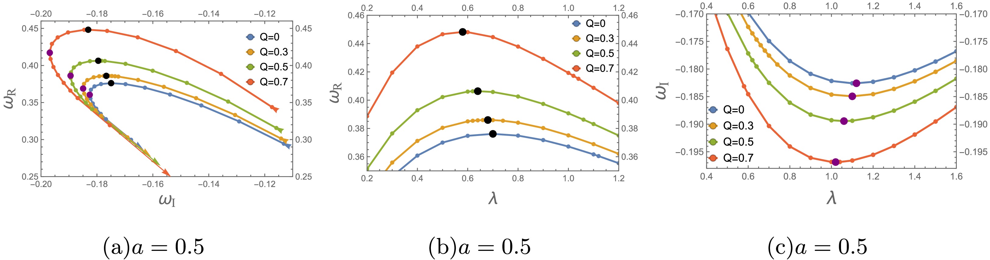

Figure 6.  (color online) Variation of the electromagnetic fundamental QNFs ($ n=0 $) as functions of λ for $ M=1 $, $ l=1 $. The arrows in panel (a) indicate the direction of increasing λ for $ \lambda\in[0.1,3] $. Black dots denote the maxima of $ \omega_{\rm{R}} $, and purple dots denote the minima of $ \omega_{\rm{I}} $ as functions of λ. Panels (b) and (c) show the decomposed real and imaginary parts, $ \omega_{\rm{R}} $ and $ \omega_{\rm{I}} $, corresponding to panel (a), respectively; the values of λ at the black and purple dots can be extracted directly from these panels.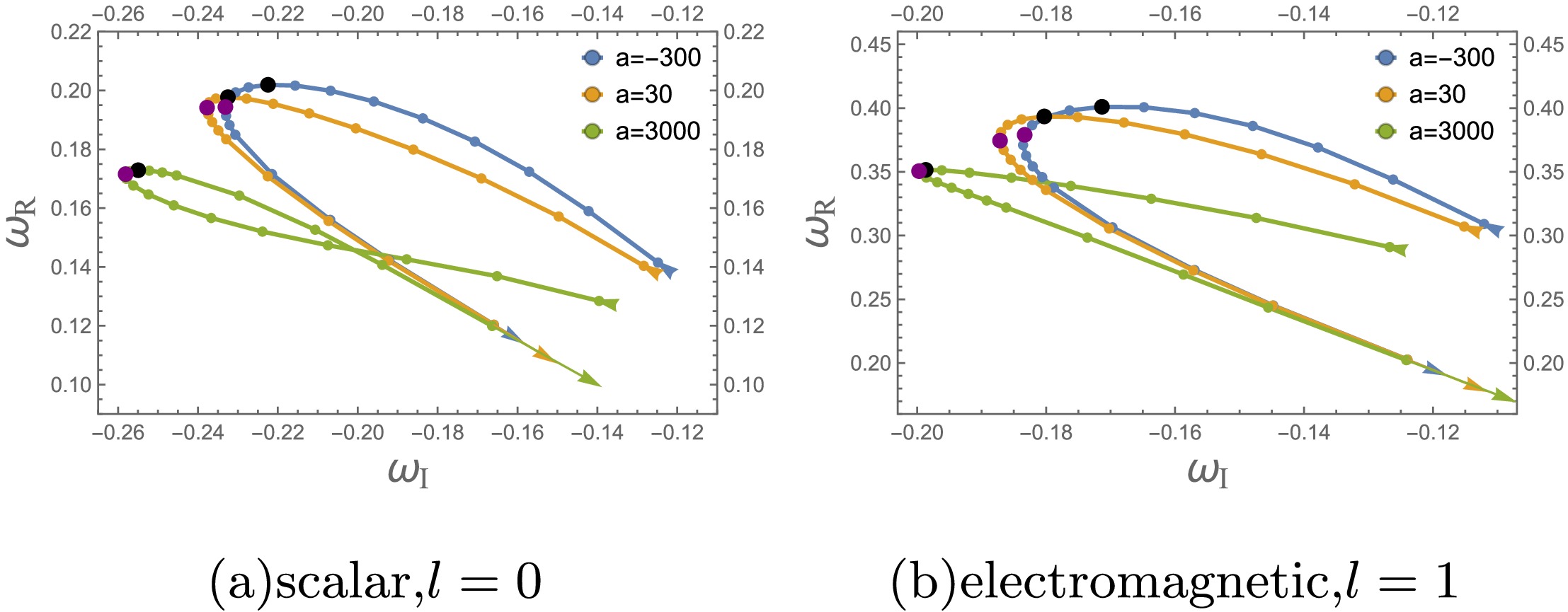

Figure 7.  (color online) Variation of the fundamental scalar and electromagnetic QNFs ($ n=0 $) with λ for $ M=1 $. The arrows in panels (a) and (b) indicate the direction of increasing λ for $ \lambda\in[0.1,4] $. Black dots denote the maxima of $ \omega_{\rm{R}} $, and purple dots denote the minima of $ \omega_{\rm{I}} $ as functions of λ. For $ a=-300,30,3000 $, the black dots are located near $ \lambda=0.86,0.92,1.27 $, respectively, and the purple dots near $ \lambda=1.3,1.21,1.1 $, respectively, in panel (a). In panel (b), the black dots are located near $ \lambda=0.67,0.73,0.8 $, respectively, and the purple dots near $ \lambda=1.1,1.03,0.9 $, respectively.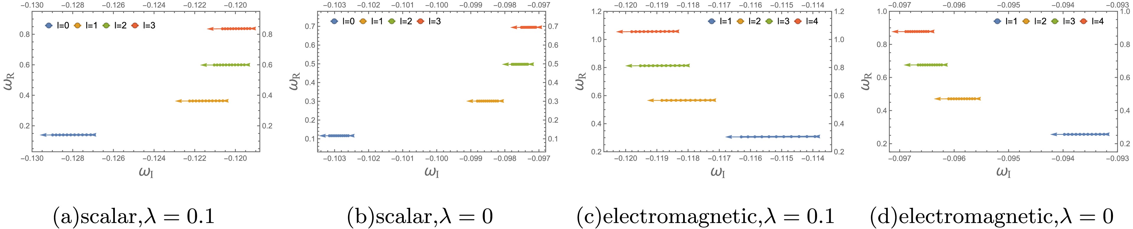

Figure 8.  (color online) Variation of scalar and electromagnetic fundamental QNFs ($ n=0 $) with parameter a for $ M=1 $ and $ Q=0.4 $. Panels (a) and (b) show scalar QNFs, while panels (c) and (d) show electromagnetic QNFs. The arrows indicate the direction in which parameter a increases. Curves with different colors correspond to distinct l values and share the same sampled values of a: $ a=-100, -80, -60, -40, -20, 0, 20, 40, 60, 80,100 $.

Figure 9.  (color online) Variation of the scalar ($ l=0 $) and electromagnetic ($ l=1 $) fundamental QNFs ($ n=0 $) as a function of the parameter a for $ M=1 $. The arrows indicate the direction of increasing a. Curves with different colors corresponding to distinct Q values share identical sampling nodes of a, with the parameter sequence $ a=-10, 20, 60,100,140,180,220,260,300 $.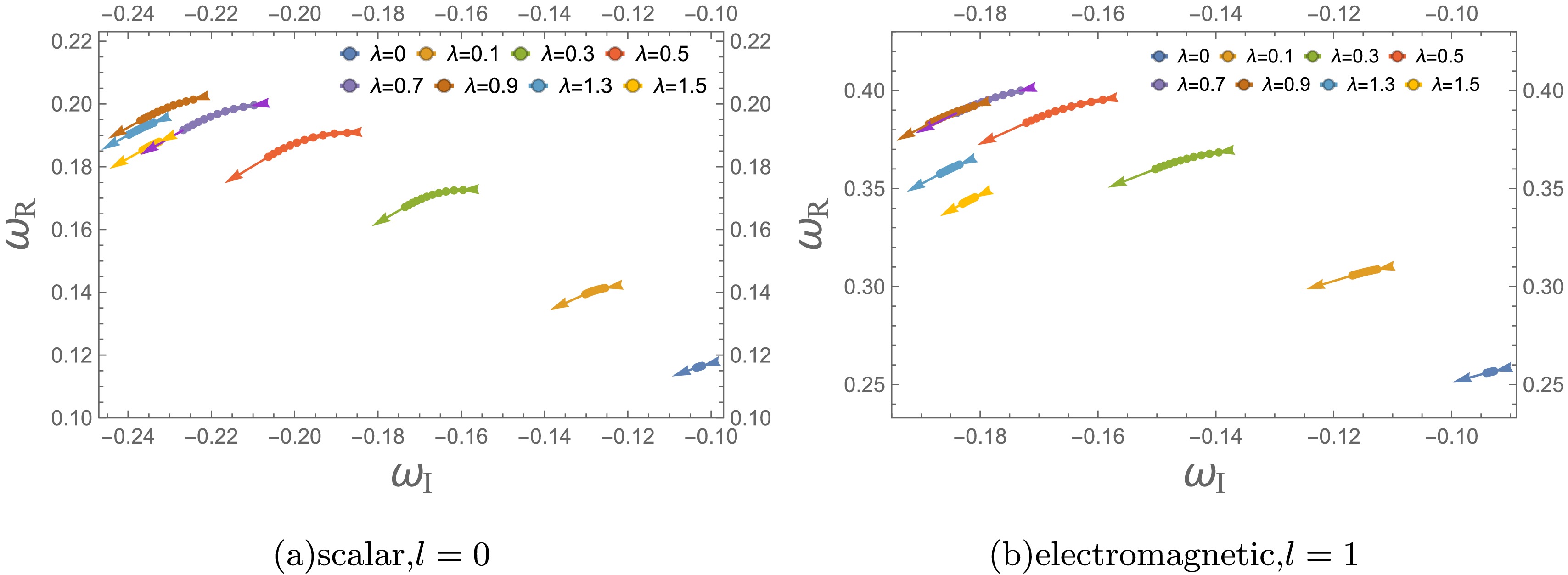

Figure 10.  (color online) Variation of the fundamental QNFs ($ n=0 $) for external fields as functions of a, for $ M=1 $ and $ Q=0.4 $. The arrows in panels (a) and (b) indicate the direction of increasing a. The sampling points on the curves, with different colors corresponding to different values of λ, are taken from the same sequence of a values: $ a=-250, -200, -150, -100, -50, 0, 50,100,150,200,250 $.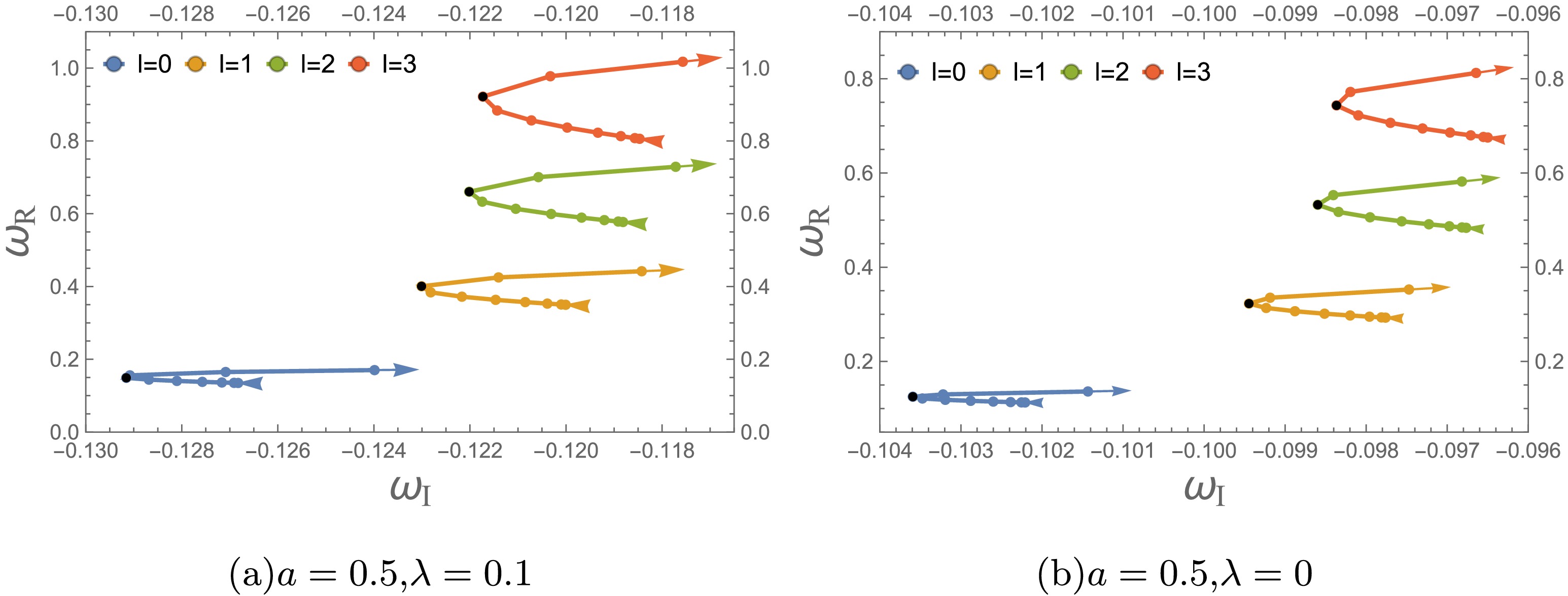

Figure 11.  (color online) Variation in the scalar fundamental QNFs ($ n=0 $) as a function of Q for $ M=1 $. The arrows in panels (a)–(d) indicate the direction of increasing $ Q\in[0,Q_c) $, where $ Q_c $ is the extremal parameter. Black dots denote the minima of $ \omega_{\rm{I}} $ as a function of Q. In (a), the black dots are near $ Q\approx0.7 $ for $ l=1,2,3 $ and $ Q\approx0.6 $ for $ l=0 $. In (b), the black dots are near $ Q\approx0.7 $ for $ l=0,1,2,3 $.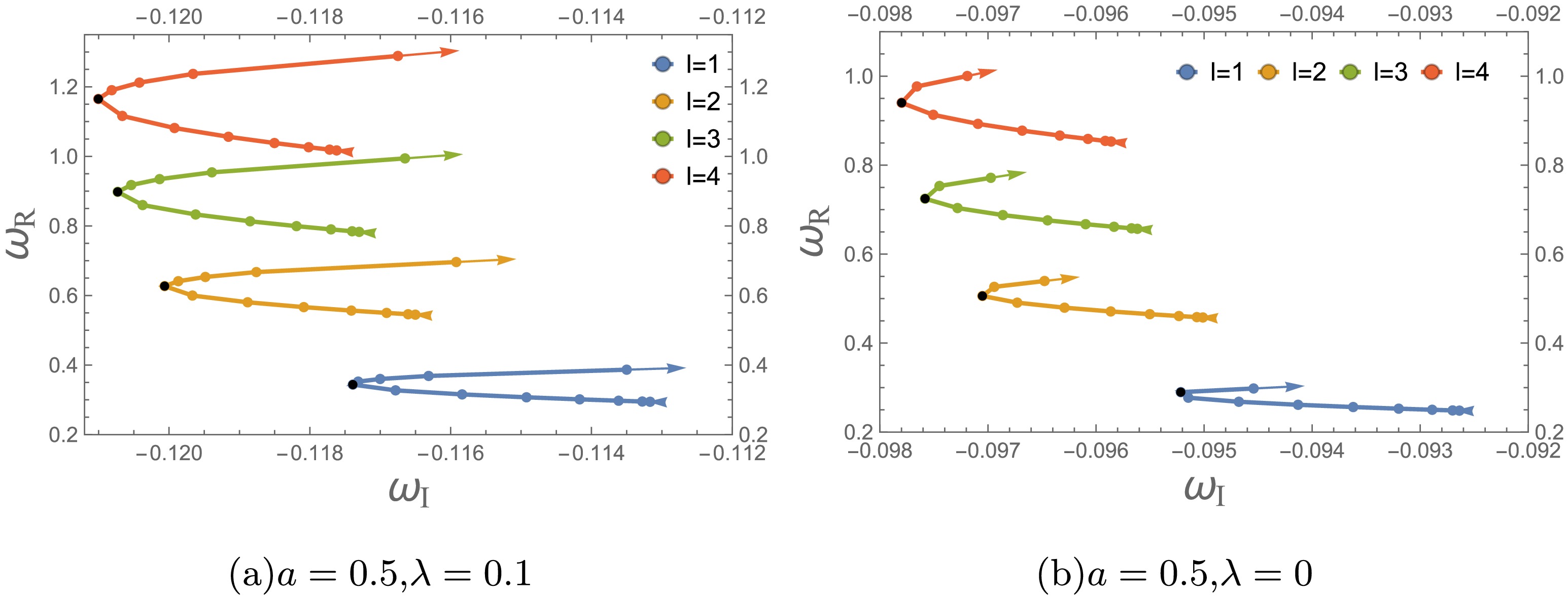

Figure 12.  (color online) Variation of the fundamental electromagnetic QNFs ($ n=0 $) as a function of different Q values for $ M=1 $. The arrows in panels (a)–(d) indicate the direction of increasing $ Q\in[0,Q_c) $, where $ Q_c $ is the extremal parameter. Black dots denote the minima of $ \omega_{\rm{I}} $ as a function of Q. In (a), the black dots occur near $ Q\approx0.7 $ for $ l=1,2,3,4 $. In (b), the black dots occur near $ Q\approx0.7 $ for $ l=2,3,4 $ and near $ Q\approx0.8 $ for $ l=1 $.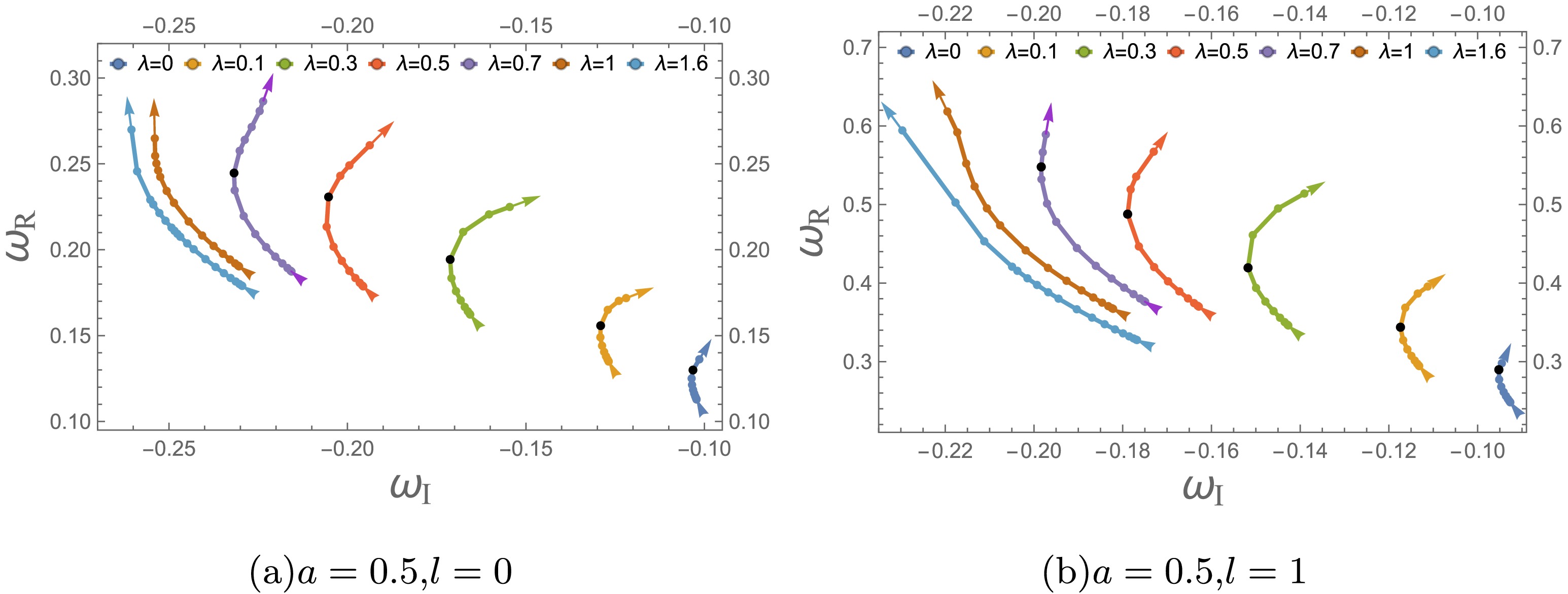

Figure 13.  (color online) Variation of the scalar ($ l=0 $) and electromagnetic ($ l=1 $) fundamental QNFs ($ n=0 $) with Q for $ M=1 $. Arrows indicate the direction of increasing $ Q\in[0,Q_c) $ ($ Q_c $ increases with λ). Black dots mark the minima of $ \omega_{\rm{I}} $ as a function of Q. For scalar QNFs, minima occur near $ Q=0.7,0.6,0.68,0.72,0.85 $ (panel (a)) for $ \lambda=0,0.1,0.3,0.5,0.7 $, respectively, with no minima for $ \lambda=1,1.6 $. For electromagnetic QNFs, minima occur near $ Q=0.8,0.69,0.71,0.8,0.92 $ (panel (b)) for the same values of λ and vanish at $ \lambda=1,1.6 $.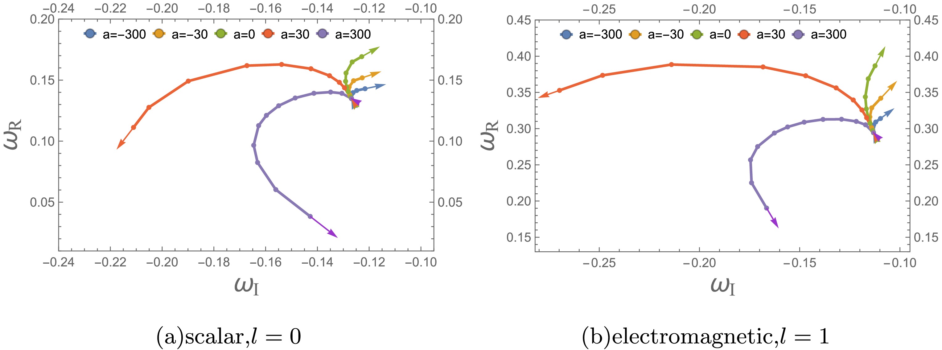

Figure 14.  (color online) Variation of the fundamental QNFs ($ n=0 $) of external fields as functions of Q, with $ M=1 $ and $ \lambda=0.1 $. The arrows in panels (a) and (b) indicate the direction of increasing $ Q\in[0,Q_{\rm{c}}) $, where the extremal parameter $ Q_{\rm{c}} $ increases with a. For the curves corresponding to $ a=-300 $, $ -30 $, $ 0 $, $ 30 $, and $ 300 $, the respective ranges of Q are $ [0,0.45] $, $ [0,0.68] $, $ [0,0.85] $, $ [0,1.6] $, and $ [0,2.4] $.

Fig. 3 presents the trajectories of the fundamental quasinormal frequencies ($ n=0 $) in the complex ω-plane for scalar ($ l=0, 1, 2, \dots, 8 $) and electromagnetic ($ l=1, 2, \dots, 8 $) perturbations as the angular momentum parameter l varies. In both perturbation sectors, increasing l shifts the QNM trajectories toward larger real parts $ \omega_{\rm{R}} $ and more negative imaginary parts $ \omega_{\rm{I}} $, indicating higher oscillation frequencies and faster damping. The same trend appears in both the PFDM background ($ \lambda=0.1 $) and the vacuum case ($ \lambda=0 $), corresponding to Fig. 3(a) and Fig. 3(b), respectively.

The scalar and electromagnetic modes exhibit qualitatively similar trajectory patterns, with both sectors showing monotonic increases in $ \omega_{\rm{R}} $ as l increases. This behavior reflects the elevation and narrowing of the effective potential barriers at higher angular momentum numbers, which strengthens the confinement of perturbation waves near the photon sphere. The systematic displacement along the trajectories indicates that higher multipole modes oscillate more rapidly and decay faster.

Comparison of the two panels in Fig. 3 shows that the PFDM environment ($ \lambda=0.1 $) systematically modifies the QNM trajectories relative to the vacuum case. It enhances both the oscillation frequency and the damping rate, consistent with the higher and narrower effective-potential barriers discussed above. This effect becomes more pronounced as l increases because the stronger angular-momentum contribution makes the spectrum more sensitive to PFDM-induced changes in the potential. The case $ a = -0.5 $ exhibits behavior qualitatively similar to that of $ a = 0.5 $; therefore, we use $ a = 0.5 $ as the representative fixed value in the following discussion, as illustrated in Fig. 3.

The fundamental quasinormal frequencies ($ n=0 $) of scalar and electromagnetic perturbations exhibit a pronounced nonmonotonic dependence on the PFDM parameter λ, as illustrated in Figs. 4–7. In both sectors, the QNM trajectories in the complex ω-plane display a characteristic hook-like structure. As λ increases, the oscillation frequency $ \omega_{\rm{R}} $ first rises to a maximum, marked by black dots, and then decreases, whereas $ \omega_{\rm{I}} $ follows the opposite trend, reaching a minimum, marked by purple dots, before increasing. This behavior indicates that PFDM initially strengthens the effective potential barrier and wave confinement, but the barrier response eventually reverses in the strong-dark-matter regime, facilitating tunneling.

A distinct difference appears in the angular-momentum dependence of these critical points, as shown in Fig. 4. For scalar perturbations in Fig. 4(a), the critical values of λ shift toward smaller values as l increases (e.g., black dots near $ \lambda \approx 0.9, 0.8, 0.77, 0.75 $). For electromagnetic perturbations in Fig. 4(b), they instead shift toward larger λ (e.g., black dots near $ \lambda \approx 0.7, 0.73, 0.75, 0.8 $). This contrast follows from the different effective-potential structures: the scalar potential contains an additional derivative term involving the metric function, whereas the electromagnetic potential is governed primarily by the centrifugal barrier. Consequently, angular momentum regulates the PFDM scale at which the QNMs reach their extrema differently in the two perturbation sectors.

The influence of the black hole charge Q on this nonmonotonic structure is shown in Figs. 5–6 for scalar ($ l=0 $) and electromagnetic ($ l=1 $) perturbations, respectively. In both sectors, increasing Q shifts the trajectories toward larger $ \omega_{\rm{R}} $ and more negative $ \omega_{\rm{I}} $, reflecting the charge-induced enhancement of the effective potential barrier. More importantly, the critical values of λ associated with the maxima of $ \omega_{\rm{R}} $ and the minima of $ \omega_{\rm{I}} $ move systematically toward smaller values as Q increases, as seen in the decomposed panels of these figures. Thus, a stronger charge causes the nonmonotonic response to emerge at a smaller PFDM parameter, increasing the spectral sensitivity to the dark-matter environment.

A strong coupling between the nonlinear parameter a and λ is further revealed in Fig. 7, where scalar ($ l=0 $) and electromagnetic ($ l=1 $) QNFs are plotted for different values of a. Increasing a shifts the critical λ for the $ \omega_{\rm{R}} $ maximum toward larger values, while moving the critical λ for the $ \omega_{\rm{I}} $ minimum toward smaller values—a trend observed in both perturbation sectors. Specifically, for $ a=-300, 30, 3000 $, the black dots are located near $ \lambda= 0.86, 0.92, 1.27 $ and the purple dots near $ \lambda=1.3, 1.21, 1.1 $ in Fig. 7(a), whereas in Fig. 7(b), the black dots are near $ \lambda=0.67, 0.73, 0.8 $ and the purple dots near $ \lambda= 1.1, 1.03, 0.9 $. This opposite displacement shows that nonlinear corrections modify the characteristic PFDM scales at which oscillation and damping reach their extrema, rather than simply rescaling the spectrum.

Taken together, Figs. 4–7 establish a clear hierarchy of parameter couplings. The PFDM parameter λ drives the nonmonotonic evolution of the QNM spectrum, the charge Q shifts the characteristic scale toward smaller values, and the nonlinear parameter a modifies the locations and ranges of the extrema. The influence of a is nevertheless suppressed in the strong-dark-matter regime, where the trajectories are dominated by λ. The observed oscillation and damping behavior therefore results from competition among the three parameters. The case $ a = -0.5 $ exhibits behavior qualitatively similar to that for $ a = 0.5 $; thus, we use $ a = 0.5 $ as the representative fixed value in the following discussion, as illustrated in Figs. 4–6.

Figure 8 illustrates the evolution of the fundamental quasinormal frequencies ($ n=0 $) in the complex ω-plane as the nonlinear Euler–Heisenberg parameter a varies. The scalar modes are shown in Fig. 8(a) and Fig. 8(b), while the electromagnetic modes are shown in Fig. 8(c) and Fig. 8(d). A universal trend emerges in both the PFDM environment ($ \lambda=0.1 $, Fig. 8(a) and Fig. 8(c)) and the vacuum case ($ \lambda=0 $, Fig. 8(b) and Fig. 8(d)): increasing a systematically shifts the QNM trajectories toward a smaller real part $ \omega_{\rm{R}} $ and a more negative imaginary part $ \omega_{\rm{I}} $, corresponding to slower oscillations and faster damping. The multipole number l further modulates this nonlinear effect. Although larger l shifts the trajectories toward higher oscillation frequencies, it simultaneously reduces the displacement induced by varying a, indicating that the centrifugal barrier suppresses the subleading geometric corrections introduced by the nonlinear parameter.

The influence of the black hole charge Q on this parameter dependence is detailed in Fig. 9. The scalar ($ l=0 $) and electromagnetic ($ l=1 $) modes are shown in Fig. 9(a)–Fig. 9(d). A larger charge Q significantly enhances the spectral sensitivity to the nonlinear parameter a, whereas the PFDM background primarily translates the trajectories in the complex plane without fundamentally altering their qualitative behavior.

The intricate interplay between the nonlinear parameter a and the dark matter parameter λ is shown in Fig. 10. The fundamental QNFs for the scalar ($ l=0 $) and electromagnetic ($ l=1 $) fields are shown in Fig. 10(a) and Fig. 10(b), respectively. The magnitude of the QNM shift induced by a depends nonmonotonically on λ: the displacement initially increases with λ but eventually saturates and weakens in the strong-PFDM regime. In this limit, the QNM trajectories form compact clusters, indicating that the perturbation dynamics are increasingly governed by the dark-matter halo and that the relative influence of a is suppressed.

This phenomenological behavior can be traced to the structure of the effective potential. The parameter a predominantly alters the near-horizon geometry, leaving the global shape of the potential barrier largely intact. Consequently, the spectral signature of a becomes most pronounced in the strong nonlinear regime and is further enhanced by a sufficiently large charge Q or a moderate dark matter density λ. Conversely, an overwhelming dark matter environment masks these nonlinear corrections. In summary, the parameter hierarchy is well defined: Q sets the primary scale for oscillation, λ determines the macroscopic environmental modifications, and a acts as a secondary, nonlinear perturbation whose observational footprint depends strongly on the ambient dark matter density and the angular momentum of the perturbed field.

In Figs. 11–14, we present the trajectories of the fundamental quasinormal frequencies ($ n=0 $) in the complex ω-plane for scalar and electromagnetic perturbations as the black hole charge Q varies. As shown in Figs. 11 and 12, the real oscillation frequency $ \omega_{\rm{R}} $ increases monotonically with Q. This behavior results from the charge-induced enhancement of the effective potential barrier and the consequent stronger confinement of perturbation waves near the photon sphere. Low-multipole perturbations are particularly sensitive to this effect. For scalar perturbations, the black dots lie near $ Q\approx0.7 $ for $ l=1,2,3 $ and near $ Q\approx0.6 $ for $ l=0 $ in Fig. 11(a), while they lie near $ Q\approx0.7 $ for $ l=0,1,2,3 $ in Fig. 11(b). For electromagnetic perturbations, the corresponding black dots lie near $ Q\approx0.7 $ for $ l=0,1,2,3 $ in Fig. 12(a); in Fig. 12(b), they lie near $ Q\approx0.7 $ for $ l=2,3,4 $ and near $ Q\approx0.8 $ for $ l=1 $. In contrast, $ \omega_{\rm{I}} $ depends nonmonotonically on Q: it first decreases to a minimum at the black dots and then increases, reflecting the competition between the barrier height and its curvature near the peak.

The influence of the dark-matter environment on this damping structure is shown in Fig. 13. Increasing λ monotonically raises $ Q_c $. Quantitatively, for scalar QNFs, minima emerge near $ Q=0.7, 0.6, 0.68, 0.72, 0.85 $ in Fig. 13(a) for $ \lambda=0, 0.1, 0.3, 0.5, 0.7 $, with no minima for $ \lambda=1, 1.6 $. For electromagnetic QNFs, minima appear near $ Q= 0.8, 0.69, 0.71, 0.8, 0.92 $ in Fig. 13(b) for the same λ values and vanish at $ \lambda=1, 1.6 $. When $ \lambda\gtrsim1 $, the nonmonotonic damping feature disappears, and $ \omega_{\rm{I}} $ becomes monotonic in Q. This transition occurs in both perturbation sectors and is nearly independent of the sign of a.

The role of the nonlinear parameter a is shown in Fig. 14. In the strongly nonlinear regime, increasing a changes the dependence of $ \omega_{\rm{R}} $ on Q from a monotonic increase to a trend that first rises and then decreases. It also makes the behavior of $ \omega_{\rm{I}} $ more complex and increases the critical charge $ Q_c $. For instance, as a increases from $ -300 $ to $ 300 $, the accessible charge range extends from $ Q\in[0,0.45] $ to $ Q\in[0,2.4] $.

Finally, a direct comparison between Figs. 11 and 12 demonstrates that scalar perturbations are more sensitive to Q than electromagnetic perturbations, owing to the additional derivative term in the scalar effective potential. Overall, Q controls the growth of the oscillation frequency and regulates the damping behavior through the curvature of the barrier, whereas λ and a reshape the damping structure and the location of the extremum charge as environmental and nonlinear parameters, respectively. The case $ a = -0.5 $ exhibits qualitatively similar behavior to $ a = 0.5 $; thus, we use $ a = 0.5 $ as the representative fixed value in the following discussion, as illustrated in Figs. 11–13.

In this section, we use the WKB approximation to calculate the greybody factors for scalar perturbations. The boundary condition for the scattering process differs from that for the QNMs and can be written as [3, 5]

where R and T represent the reflection and transmission coefficients, respectively. The greybody factor is defined as the probability that an outgoing wave reaches infinity or that an incoming wave is absorbed by the black hole [45−47]. Therefore, $ |T(\omega)|^2 $ is the greybody factor, and $ R(\omega) $ and $ T(\omega) $ should satisfy the following relation:

The reflection and transmission coefficients can be obtained using the sixth-order WKB method [35, 44].

where K is a parameter that can be obtained using the WKB formula [35]

In Figs. 15 and 16, we present the greybody factors $ |T(\omega)|^2 $ for scalar and electromagnetic perturbations ($ l=1 $) for varying charge Q. For both PFDM ($ \lambda=0.1 $) and vacuum ($ \lambda=0 $) backgrounds, increasing Q systematically shifts the transmission curves to higher frequencies and suppresses the greybody factor, reflecting the monotonic enhancement of the effective potential barrier. The influence of the nonlinear parameter a is shown in Figs. 17 and 18; varying a produces only minor modifications confined to the low-frequency region, consistent with its localized near-horizon corrections.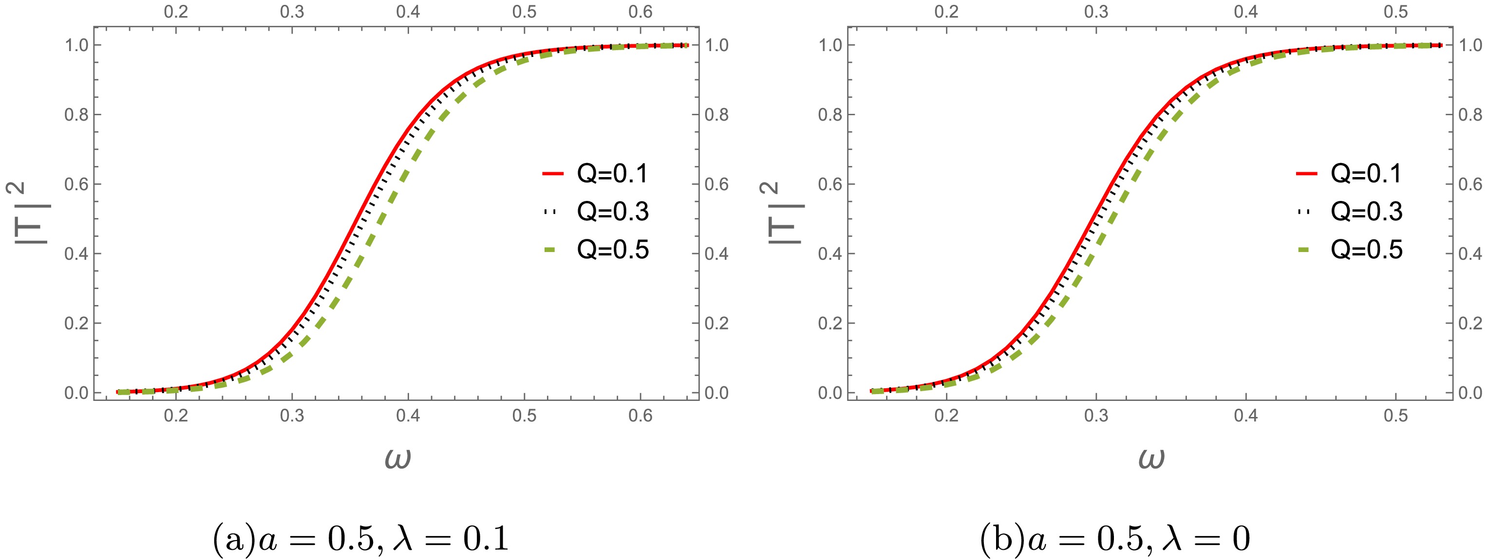

Figure 15.  (color online) Scalar-field greybody factor as a function of Q for $ M=1 $ and $ l=1 $.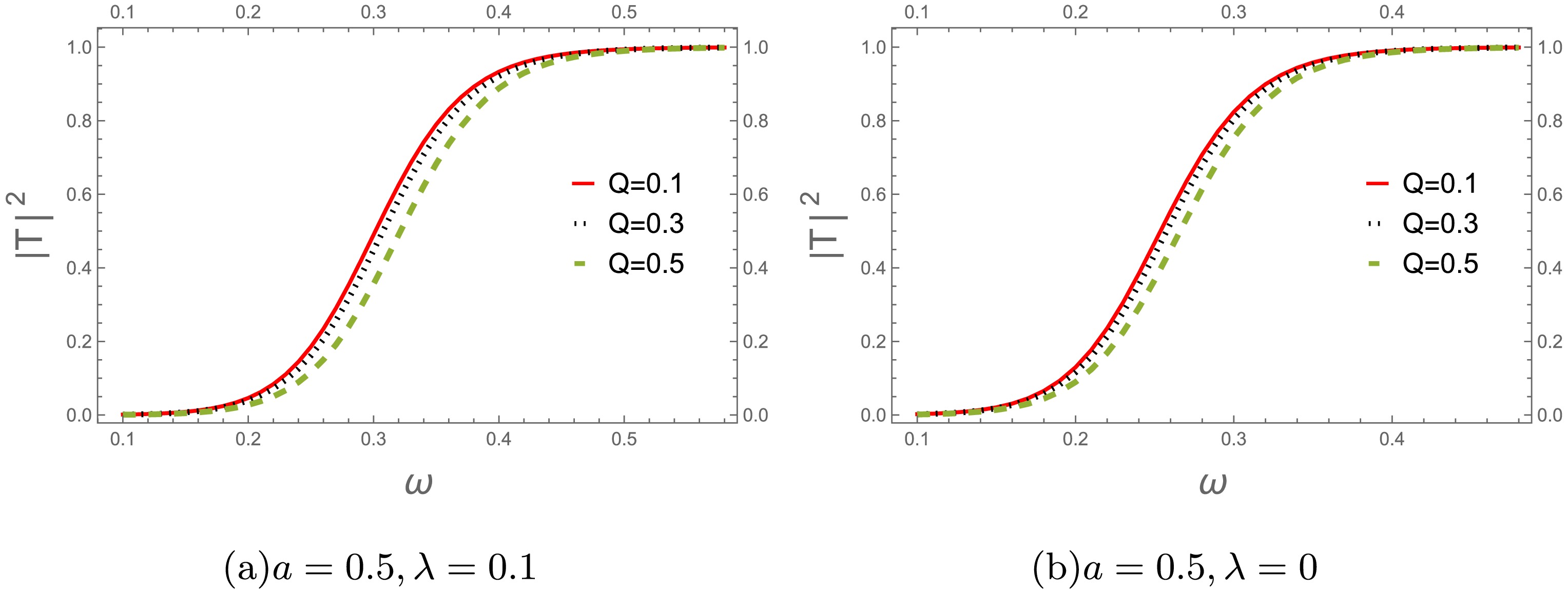

Figure 16.  (color online) Electromagnetic field greybody factor as a function of Q for $ M=1 $ and $ l=1 $.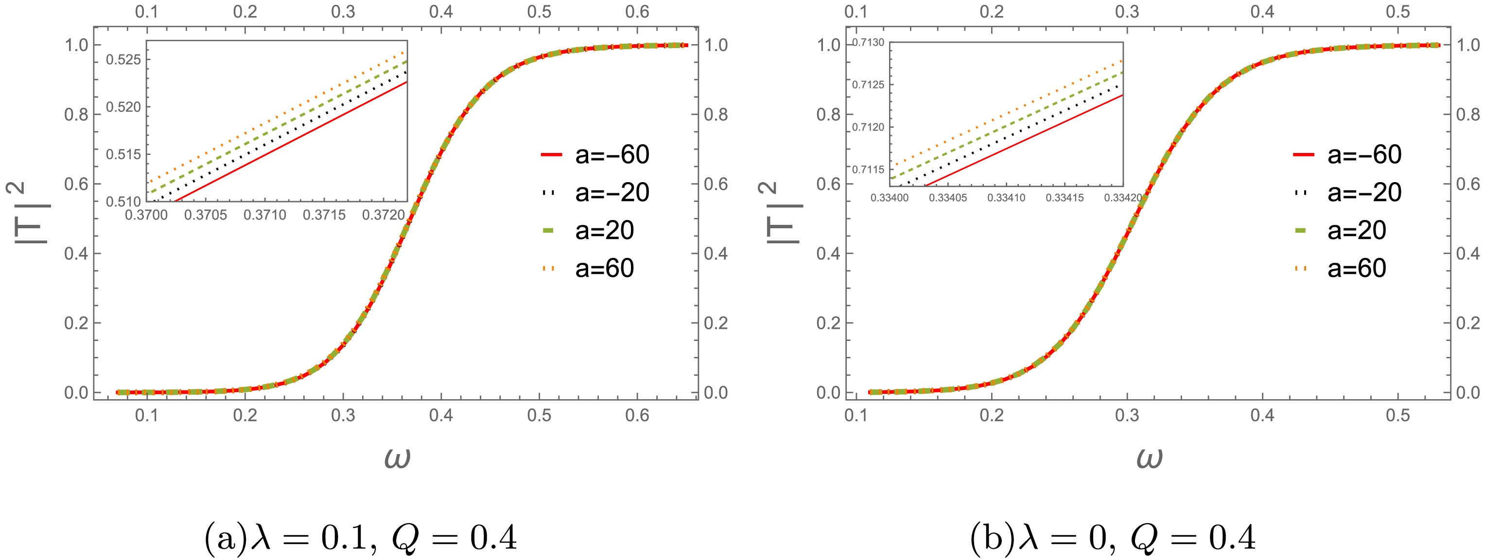

Figure 17.  (color online) The scalar field greybody factor vs. a for $ M=1 $ and $ l=1 $.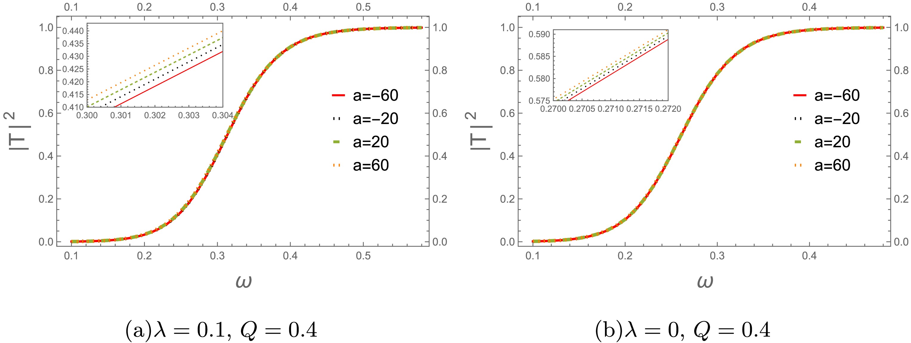

Figure 18.  (color online) The electromagnetic-field greybody factor as a function of a for $ M=1 $ and $ l=1 $.

The dependence on the PFDM parameter λ is detailed in Figs. 19 and 20. In the weak- and moderate-PFDM regimes (Figs. 19(a) and 20(a)), increasing λ suppresses low-frequency transmission and shifts the transition region toward higher ω, indicating a strengthened barrier. However, in the strong-PFDM regime (Figs. 19(b) and 20(b), $ \lambda \gtrsim 1.4 $), the curves exhibit a reverse shift with increased transmission probability. This nonmonotonic behavior directly reflects the lowering and broadening of the effective potential barrier in the strong-dark-matter regime, which facilitates wave tunneling.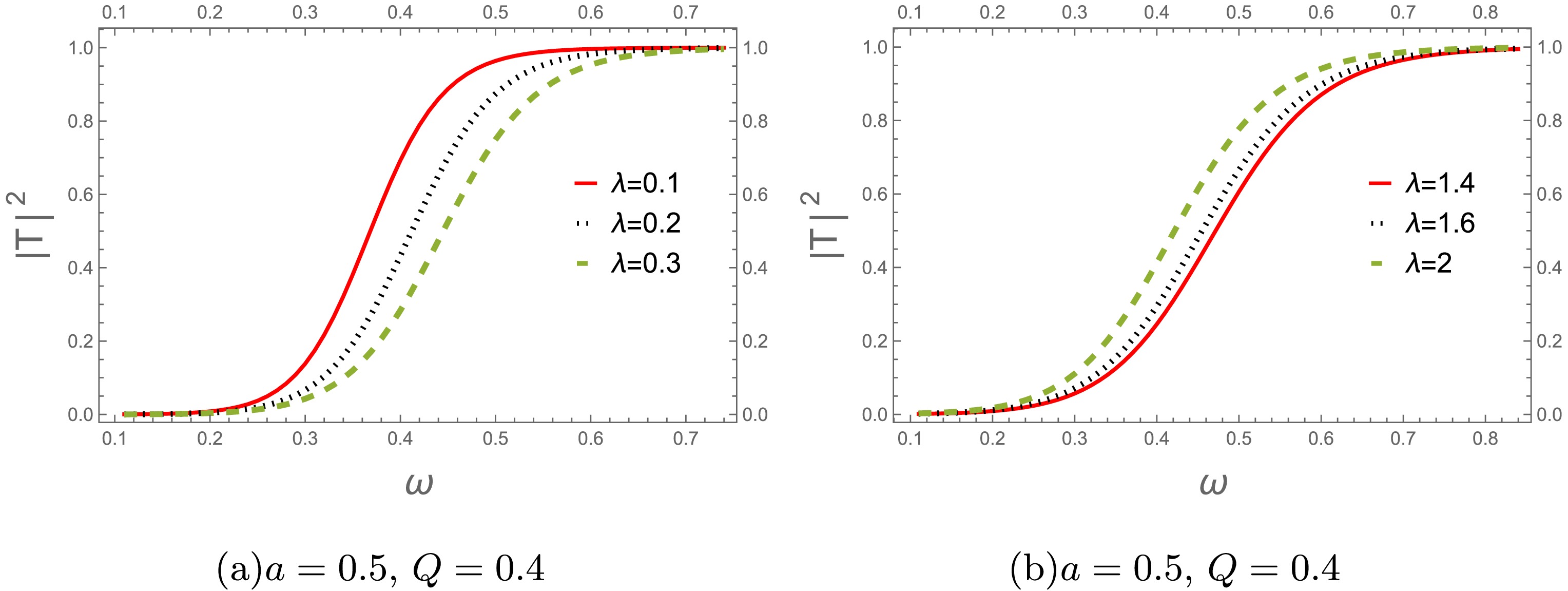

Figure 19.  (color online) The scalar-field greybody factor as a function of λ for $ M=1 $ and $ l=1 $.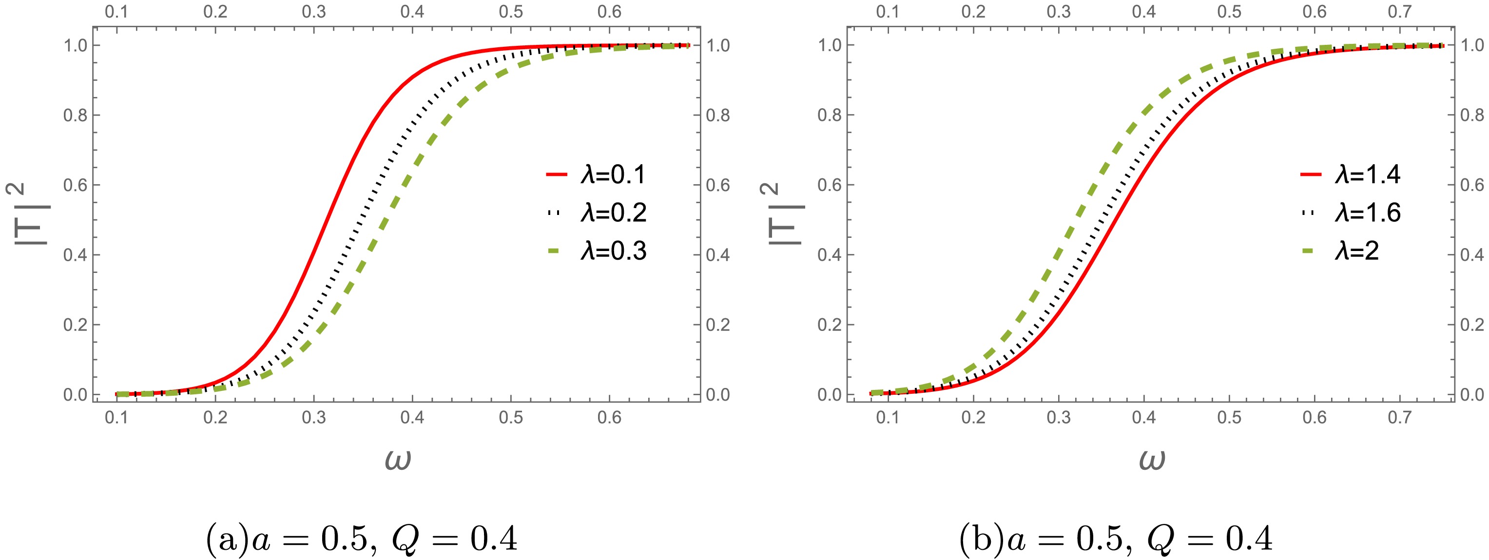

Figure 20.  (color online) Electromagnetic-field greybody factor as a function of λ for $ M=1 $ and $ l=1 $.

Comparison of Figs. 15–20 shows that Q and λ significantly regulate the transmission probability, whereas a acts as a subleading correction. Both perturbation sectors exhibit qualitatively similar behavior, indicating that the dominant features are governed by the background geometry rather than by the field spin. Overall, the suppression of low-frequency transmission indicates barrier strengthening by Q and weak-to-moderate λ, whereas the reverse shift for $ \lambda \gtrsim 1.4 $ confirms barrier lowering in the strong-dark-matter regime. As illustrated in Figs. 15–16 and 19–20, we adopt $ a=0.5 $ as the representative value, having verified that $ a=-0.5 $ yields qualitatively similar results.

In this work, we systematically investigate the quasinormal modes (QNMs) and greybody factors of massless scalar and electromagnetic perturbations around the Euler–Heisenberg black hole surrounded by perfect fluid dark matter (PFDM). Using the asymptotic iteration method (AIM) together with the sixth-order WKB approximation, we analyze the effects of the black hole charge Q, the PFDM parameter λ, and the nonlinear Euler–Heisenberg parameter a on the dynamical properties of the spacetime. The excellent agreement between the AIM and WKB results confirms the reliability and accuracy of the obtained quasinormal spectra.

The effective potential analysis shows that both the black hole charge and the PFDM environment significantly modify the structure of the scattering barrier. Increasing the charge parameter Q generally increases the height of the effective potential barrier for both scalar and electromagnetic perturbations, leading to stronger confinement of perturbative waves near the photon-sphere region. By contrast, the PFDM parameter λ has a more intricate influence on the effective potential. In the weak-PFDM regime, increasing λ raises and sharpens the effective potential barrier, whereas for sufficiently large values of λ, the barrier becomes lower and smoother, reducing the curvature near the potential peak. The nonlinear Euler–Heisenberg correction primarily affects the near-horizon geometry and becomes prominent in the strong nonlinear regime.

The quasinormal spectra exhibit several remarkable dynamical features. For moderate values of the nonlinear parameter a, the oscillation frequency $ \omega_{\rm{R}} $ increases monotonically with Q, while the damping magnitude $ |\omega_{\rm{I}}| $ exhibits a characteristic nonmonotonic dependence, reaching a clear minimum at the critical charge $ Q_c $, i.e., at extremality. This behavior originates from the competition between the height and curvature of the effective potential near its peak. The PFDM parameter λ increases $ Q_c $, and sufficiently strong dark matter can even eliminate the nonmonotonic damping behavior entirely. These results indicate that environmental dark matter effects can qualitatively alter the ringdown properties of charged black holes.

A comparison between scalar and electromagnetic perturbations reveals that scalar modes are generally more sensitive to the background geometry and the PFDM environment. This distinction arises because the scalar effective potential contains an additional derivative term $ rf(r)f'(r) $, whereas the electromagnetic potential depends only on the centrifugal contribution. Consequently, scalar perturbations exhibit stronger variations in both oscillation frequency and damping rate under changes in the spacetime parameters. Nevertheless, both fields share consistent qualitative behavior, demonstrating the universality of the underlying physical mechanism.

In the strong nonlinear regime, the Euler–Heisenberg correction introduces qualitatively new effects into the quasinormal dynamics. The dependence of $ \omega_{\rm{R}} $ on Q gradually changes from a monotonic increase to a trend of initially increasing and then decreasing near extremality. Meanwhile, the damping structure becomes more complex, indicating that strong nonlinear electrodynamic effects substantially reshape the curvature of the effective potential near its peak. A robust result is that the critical charge $ Q_c $ increases monotonically with a, demonstrating that stronger nonlinear corrections push the extremal condition toward larger black hole charge.

From a physical perspective, the parameter λ determines the density and distribution of the perfect fluid dark matter halo surrounding the black hole. As λ increases in the weak-PFDM regime, the dark matter distribution introduces an additional effective gravitational dragging effect, which pulls the peak of the effective potential outward and sharpens it. This leads to a higher oscillation frequency. However, in the strong-PFDM regime (large λ), the background geometry becomes strongly dominated by the dark matter fluid, flattening the spacetime curvature near the photon sphere. This physical competition explains the nonmonotonic behavior observed in the damping rate $ \omega_{\rm{I}} $. We consider λ to be the most relevant parameter in our study, as it determines the macroscopic deviation from standard vacuum general relativity.

The greybody-factor analysis further confirms the close connection between scattering properties and the effective potential structure. Increasing Q suppresses low-frequency transmission, while λ regulates wave confinement and tunneling. Both nonlinear electrodynamics and PFDM leave characteristic imprints on black hole absorption and scattering, which may be detectable in future observations.

Overall, the interplay between black hole charge, nonlinear electrodynamics, and perfect fluid dark matter yields rich and nontrivial modifications to quasinormal spectra and greybody factors. The competition between the height and curvature of the effective potential governs the oscillation and damping characteristics of perturbative modes. Our results provide valuable theoretical templates for future gravitational-wave observations, black hole spectroscopy, and tests of strong-field gravity and nonlinear electrodynamics in dark matter environments. In particular, the recently proposed gravitational-wave–black hole imaging correspondence for modified black holes [33] offers a promising framework for connecting our quasinormal mode predictions with future Event Horizon Telescope observations.

We remark that two recent investigations have addressed greybody factors in the same Euler–Heisenberg black hole spacetime surrounded by PFDM [49, 50]. While both works provide important contributions, they are constrained by their respective methodologies: the rigorous lower-bound approach [49] cannot yield exact transmission probabilities, and the eikonal approximation [50] is restricted to the large-l limit. Our work was conducted independently and complements these studies in several fundamental respects. First, by employing the sixth-order WKB approximation, we compute greybody factors at finite angular momenta ($ l = 1 $), providing quantitative transmission probabilities that go beyond both the rigorous bounds and the eikonal limit. Second, within a unified WKB framework, we identify new physical features inaccessible to the aforementioned methods. Most notably, we reveal the nonmonotonic transition of greybody factors induced by the lowered potential barrier in the strong-PFDM regime ($ \lambda \gtrsim 1.4 $), the nonmonotonic dependence of quasinormal frequencies on λ, and the critical charge $ Q_c $ structure in the damping rate. These results demonstrate that our combined QNM and greybody analysis provides complementary and, in certain aspects, more detailed information than the lower-bound or eikonal approaches, thereby significantly enriching the theoretical understanding of black hole scattering in nonlinear electrodynamic and dark matter environments.

The asymptotic iteration method (AIM) provides a stable and accurate semi-analytic strategy for solving second-order linear ordinary differential equations governing black-hole perturbations [34, 48]. This appendix outlines the full implementation of AIM for computing quasinormal frequencies, with all key equations retained in their original form.

We begin by introducing a compactified radial coordinate

This maps the exterior region $ r\in[r_{+},\infty) $ onto $ u\in[0,1) $. Substituting this transformation into the radial perturbation equation yields the following second-order ordinary differential equation in terms of u:

This second-order differential equation governs the radial behavior of perturbations and serves as the starting point for the AIM procedure.

We first analyze the asymptotic behavior near the horizon, $ u\to0 $. The metric function can be expanded to linear order as $ f(u)\approx u f'(0) $. Substituting this expression into (A1) yields the simplified equation

whose general solution is

The physically ingoing boundary condition requires $ C_{2}=0 $.

Next, we consider the asymptotic form at spatial infinity, $ u\to1 $. In this limit, the equation reduces to

Upon introducing $ \zeta=\dfrac{i r_{+}\omega}{1-u} $, the solution becomes

The purely outgoing boundary condition imposes $ D_{1}=0 $.

We now construct a global ansatz satisfying both boundary conditions:

where $ \chi(u) $ is regular on $ (0,1) $. Substituting (A6) into (A1) rewrites the equation in the canonical AIM form [34, 48]:

For scalar perturbations, the initial iteration coefficients are given by

and

For electromagnetic perturbations, the coefficient $ \lambda_{0}(u) $ is unchanged:

while $ s_{0}(u) $ takes the form

The iteration is then repeated recursively until convergence, yielding robust, high-precision quasinormal frequencies.

The sixth-order Wentzel–Kramers–Brillouin (WKB) approximation provides a reliable semianalytic method for computing quasinormal-mode frequencies and greybody factors in black hole perturbation theory [35]. This approach approximates the perturbed field equation near the peak of the effective potential barrier, where the field exhibits its dominant oscillatory behavior.

The central condition that determines the quasinormal-mode frequencies is given by

where $ n=0,1,2,\dots $ labels the overtone number. Here, $ V_0=V(r_0) $ denotes the value of the effective potential at its maximum $ r=r_0 $, and $ V_0'' $ denotes the second derivative at the peak, characterizing the curvature of the potential barrier. The terms $ \Lambda_k $ represent higher-order corrections derived from the k-th derivatives of $ V(r) $ at $ r_0 $, which systematically improve the accuracy up to sixth order.

Unlike lower-order expansions, the sixth-order scheme reliably captures the local structure of the potential near the peak, yielding accurate frequencies even in moderately strong-field regimes [35]. This method is computationally efficient and consistent with the asymptotic iteration method [34], especially for modes satisfying $ l\ge n $, for which the potential barrier is sufficiently pronounced and the WKB expansion converges rapidly. The same framework is used to compute greybody factors by evaluating the transmission probability across the potential barrier.