Phenomenological advantages of the normal neutrino mass ordering

1. Introduction

• 1. Introduction
• 2. The solar octant
• 3. The two Majorana CP phases
• 4. Conclusion

The neutrino oscillation [1, 2] is the first established new physics beyond the Standard Model (SM) of particle physics [3], although it is not clear whether it is due to a genuine mass or just an environmental matter effect [4–9]. In the last 20 years, various neutrino experiments have made impressive progresses by measuring the neutrino mixing angles and two mass splittings [10, 11]. The neutrino oscillation (mixing and mass splitting) patterns are coherently weaved, to be wise after the event. In 1995, S. Wojcicki pointed out that there seems to be an intelligent design of neutrino parameters [12], as a "light-hearted argument" [13]: 1) The solar splitting $\Delta m^2_s \equiv \Delta m^2_{21} =$$7.39^{+0.21}_{-0.20} \times 10^{-5}\,{\rm{eV}}^2$ is at the right scale to have the MSW resonance [14–17]; 2) The solar angle $\theta_s \equiv \theta_{12} = {33.82^\circ}^{+0.78^\circ}_{-0.76^\circ}$ takes the right choice to have sufficiently large oscillations ($\sim 0.8$) at KamLAND; 3) The atmospheric splitting $\Delta m^2_a \equiv \Delta m^2_{31} = 2.528^{+0.029}_{-0.031} \times 10^{-3}\,{\rm{eV}}^2$ allows full oscillation in the middle range of possible distances travelled by atmospheric neutrinos; 4) The atmospheric angle $\theta_a \equiv \theta_{23} = {48.6^\circ}^{+1.0^\circ}_{-1.4^\circ}$ is big enough so that oscillations could be easily seen; 5) The reactor angle $\theta_r \equiv \theta_{13} =$ ${8.60^\circ} \pm 0.13^\circ$ is small enough so as not to confuse the above measurements, but nevertheless large enough to allow the leptonic CP phase and mass ordering (MO) measurements. The recent T2K and NOνA data indicates a nearly maximal Dirac CP phase, $\delta_{\rm{D}} = {221^\circ}^{+39^\circ}_{-28^\circ}$, which is also a good sign. All the quoted best-fit and uncertainty values are obtained with the normal ordering (NO), $m_1^{}<m_2^{}<m_3^{}$.

The only exception comes from the neutrino MO. According to the global fit [10, 11] and cosmological constraint [18], NO is preferred [10]. This is especially notunderstandable, in contrast to the coherent picture of mixing angles and mass splittings described above. With NO, the neutrinoless double beta ($0 \nu 2 \beta$) decay has a sizeable chance ($\gtrsim$1% for $|m_{ee}| \leqslant 1\,{\rm{meV}}$) to fall into the funnel region [19] and hence becomes invisible. Even if the effective mass $|m_{ee}|$ is not inside the funnel region, it is still much more difficult to measure the $0 \nu 2 \beta$ decay with NO. A naive expectation is that the inverted ordering (IO), $m_3^{}<m_1^{}<m_2^{}$, is a better choice. Why make it difficult to measure the Majorana nature of neutrinos after paving the way for measuring the oscillation patterns? Especially, the Majorana nature is theoretically well motivated. While the mixing angles and mass splittings are essentially model parameters [20], the Majorana nature is driven by the seesaw mechanisms [21–33], leptogenesis [34], and charge quantization [35, 36]. If there is an intelligent design behind the established oscillation patterns, it is hard to imagine that the $0 \nu 2 \beta$ decay for measuring the Majorana nature is left unattended. Thus, choosing the NO is hence dubbed as "God's Mistake" [13].

This naive expectation is not necessarily true, and we provide two arguments. The NO makes it possible to exclude the higher solar octant and simultaneously measure the two Majorana CP phases. Note that the so-called "intelligent design" [12] and "God's mistake" [13] are just triggers of our thinking and should not be considered as the logic starting point or ingredient of our scientific argument. In this paper, we try to explore the phenomenological potentials of the $0 \nu 2 \beta$ decay experiments with the NO, rather than making predictions on which mass ordering should be correct.

2. The solar octant

• 1. Introduction
• 2. The solar octant
• 3. The two Majorana CP phases
• 4. Conclusion

In the presence of the vector type non-standard interaction (NSI), the solar octant becomes obscured by the degeneracy with MO, the Dirac CP phase, and for high energy experiments also the $\epsilon_{ee}$ element from the vector NSI [37]. To make it clear, we parametrize the neutrino mixing matrix as $V_\nu = U_{23}(\theta_a) U_{13}(\theta_r) U_{12}(\theta_s, \delta_{\rm{D}})$ and the Hamiltonian as

where $D_{\nu}^{2} \equiv {\rm{diag}}\{- \dfrac{ 1} {2} \Delta m^2_s, \dfrac {1}{ 2} \Delta m^2_s, \Delta m^2_a - \dfrac {1}{ 2} \Delta m^2_s\}$ is the diagonal mass matrix. Note that parametrizing the Dirac CP phase $\delta_{\rm{D}}$ in the 1–2 mixing $U_{12}(\theta_s, \delta_{\rm{D}})$ is equivalent to the conventional parametrization [3] in the 1–3 mixing, up to a rephasing matrix on each side of $V_\nu$. For simplicity, only the real $\epsilon_{ee}$ element of the vector NSI is considered since the others are not relevant. The vacuum term ${\cal{H}}_{\rm{vac}}$ of Eq. (1), i.e., the first term on the right side of the equation, changes into $- {\cal{H}}^*_{\rm{vac}}$ under the transformation: $\sin \theta_s \leftrightarrow \cos \theta_s$, $\delta_{\rm{D}} \rightarrow \pi - \delta_{\rm{D}}$, and $\Delta m^2_a \rightarrow - \Delta m^2_a + \Delta m^2_s$^① [37]. For the matter potential term, the minus sign comes from $\epsilon_{ee} \rightarrow - 2 - \epsilon_{ee}$. Without breaking this degeneracy, the solar mixing angle has two solutions in the lower or higher octant, respectively.

Although neutrino scattering data can help to break the degeneracy to some extent [38–40], it can only apply to suffciently heavy mediators. The HO (LMA-dark) solution [41, 42] is not uniquely related to heavy mediators but can also be contributed by light mediators since their NSI effects are proportional to coupling over mass, something like $g^2 / m^2$. By proportionally adjusting coupling and mass, there is no particular mass scale for NSI. Especially, for light mediators [43–48], it is always possible to tune the coupling $g$ to be small enough to evade those experimental searches with sizeable momentum transfer including the coherent scattering experiments, since the propagator $g^2 / (q^2 - m^2) \approx g^2/q^2$ can be highly suppressed by the tiny $g$ [49–51].

In this paper, we discuss how to exclude the solar HO solution by the $0 \nu 2 \beta$ decay measurement with the help of the precision measurement at the reactor neutrino oscillation experiments, which can apply universally to both light and heavy mediators. Since the $0 \nu 2 \beta$ decay is free of NSI, and the reactor neutrino oscillation with very low energy is not sensitive to matter effects [52], to which the NSI effect belongs, their combination can provide an independent check for the aforementioned degeneracy. In Ref. [53], the authors have pointed out that the effective mass has different distributions in the LO and HO cases. Especially, the HO case can be readily measured and sets a new sensitivity goal. Their conclusion also briefly mentioned the possible 'refutal' of the HO. This section elaborates the aspect of excluding the HO solution. Especially, we stress the crucial role played by the precision measurements of reactor neutrino experiments JUNO and Daya Bay in significantly reducing the uncertainty of relevant oscillation parameters ($\theta_r$, $\theta_s$, $\Delta m^2_a$, and $\Delta m^2_s$). In addition, we discuss in detail how the cosmological mass sum can also help to exclude the HO solution once combined.

The octant transformation, $c_s \leftrightarrow s_s$ where $(c_x, s_x) \equiv$$(\cos \theta_x, \sin \theta_x)$, is actually equivalent to $m_1 \leftrightarrow m_2$. The effective mass $m_{ee}$ for the $0 \nu 2 \beta$ decay is,

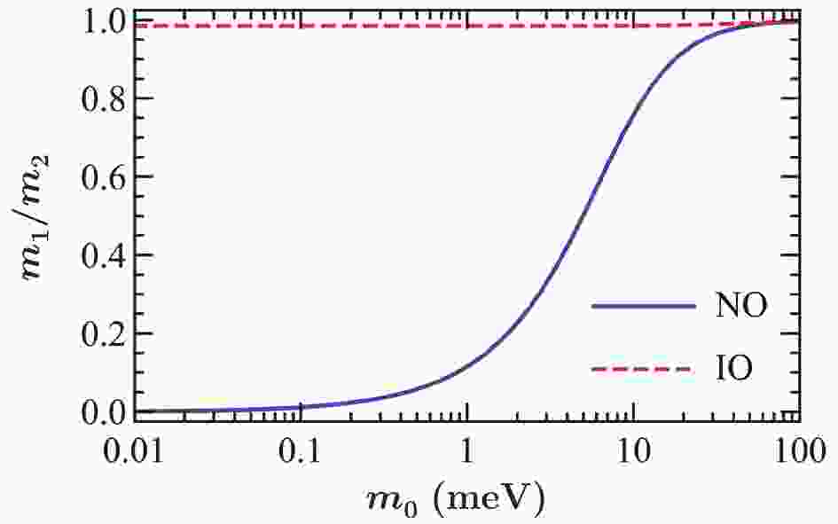
where $\tilde \delta_{\rm{Mi}} \equiv \delta_{\rm{Mi}} - \delta_{\rm{D}}$ is a combination of the Majorana CP phase $\delta_{\rm{Mi}}$ and the Dirac phase $\delta_{\rm{D}}$. Note that this form is the same as the conventional parametrization with two complex phases attached to the $m_1$ and $m_3$ terms. Although the $m_2$ term has no complex phase, it plays an equal role as the $m_1$ term, since both are vectors on the complex plane. This becomes more transparent by simply rotating the phase ${\rm e}^{{\rm i} \tilde \delta_{\rm{M3}}}$ away from the $m_3$ term, rendering both the $m_1$ and $m_2$ terms complex. Since the two Majorana CP phases $\tilde \delta_{\rm{Mi}}$ are unknown and can take any values, the effective mass $|m_{ee}|$ distribution is invariant under the combined switch $c^2_s m_1 \leftrightarrow s^2_s m_2$. The effect of $c_s \leftrightarrow s_s$ is the same as $m_1 \leftrightarrow m_2$. A direct consequence is that, if $m_1 \simeq m_2$, the octant transformation $c_s \leftrightarrow s_s$ would leave no significant consequence in the $0 \nu 2 \beta$ decay. Since the two Majorana CP phases are completely free, the transformation of the Dirac CP phase, $\delta_{\rm{D}} \rightarrow \pi - \delta_{\rm{D}}$, can be easily absorbed into its Majorana counterparts. To see the effect of switching the solar octants, the two mass eigenvalues have to be non-degenerate, which also applies for the beta decay where the key parameter is $m_\beta \equiv c^2_r c^2_s m_1 +$$c^2_r s^2_s m_2 + s^2_r m_3$ [54].

The Fig. 1 shows the ratio of $m_1/m_2$ as a function of the lightest mass, $m_0 \equiv m_1$ for NO and $m_0 \equiv m_3$ for IO. Since the atmospheric mass splitting is much larger than the solar one, $\Delta m^2_s / \Delta m^2_a$≈ 3% << 1, $m_1$ and $m_2$ are almost degenerate across the whole parameter space for IO. In contrast, they can be non-degenerate for NO. With $m_1 \lesssim 40\,{\rm{meV}}$, there is apparent deviation from being degenerate. The smaller $m_1$, the bigger the deviation.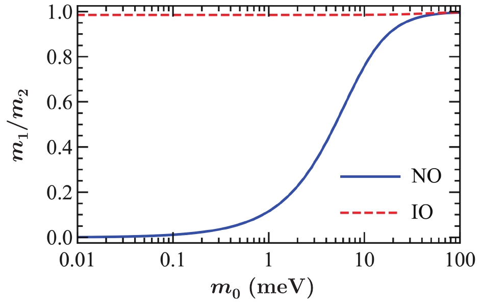

Figure 1

Figure 1.  (color online) The mass ratio $m_1 / m_2$ for NO and IO.

DownLoad: Full-Size Img PowerPoint

As expected, there is no visible difference between the solar octants for IO while for NO the effect is sizeable, as shown in Fig. 2. For IO, the predictions with LO and HO almost completely overlap with each other. So, we show only one case in green color and label it as "IO". For NO, the prediction with LO (in red color and labeled as "NO-LO") is totally different from the one with HO (in blue color and labeled as "NO-HO"). Especially, the funnel region for NO-LO completely disappears for NO-HO. Instead, the effective mass $|m_{ee}|$ is bounded from below across the whole parameter range. The different effective mass distributions between NO-LO and NO-HO as well as the degenerate distributions between IO-LO and IO-HO [53] is actually a reflection of the $m_1$–$m_2$ non-degeneracy or degeneracy, respectively.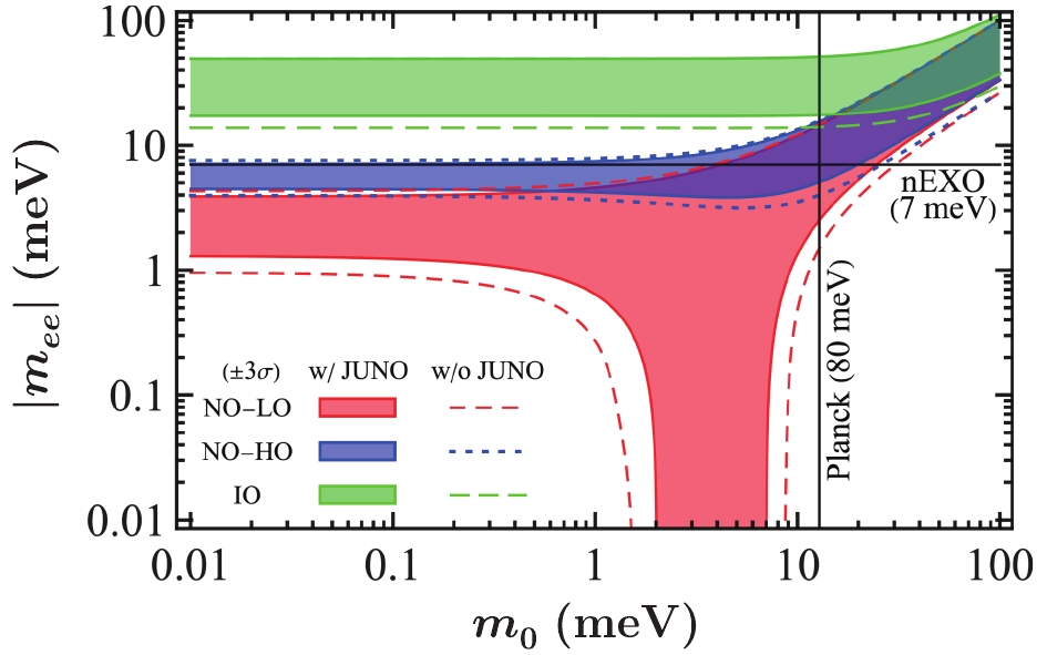

Figure 2

Figure 2.  (color online) The allowed range of $|m_{ee}|$ for NO with LO (NO-LO, red), NO with HO (NO-HO, blue), and IO (green). The dashed lines indicate the $3\sigma$ uncertainty according to the current global fit [10, 11] of neutrino oscillation parameters ($\theta_s$, $\theta_r$, $\Delta m^2_s$, and $\Delta m^2_a$) while for the filled region we further impose the projected precision of $\sin^2\theta_s$ (0.54%) and $\Delta m_s^2$ (0.24%) at the future JUNO experiment [60]. For comparison, the typical future prospects of the $0 \nu 2 \beta$ decay measurement [55] and cosmological constraint [18, 56] are shown as horizontal and vertical lines, respectively.

DownLoad: Full-Size Img PowerPoint

According to the geometrical picture [57], the lower and upper limits are completely determined by the lengths of the three complex vectors, ($L^{\rm{LO}}_1 \equiv c^2_r c^2_s m_1$, $L^{\rm{LO}}_2 \equiv c^2_r s^2_s m_2$, and $L_3 \equiv s^2_r m_3$ for LO). With $m_1$ and $m_2$ switched, namely $L^{\rm{HO}}_1 \equiv c^2_r s^2_s m_1$ and $L^{\rm{HO}}_2 \equiv c^2_r c^2_s m_2$ for HO, the situation becomes totally different from the LO case. For convenience, we use only the LO value for the solar angle, $\theta_s < \pi/4$, globally. As shown in Fig. 3, $L^{\rm{HO}}_2 > L^{\rm{HO}}_1 + L_3$ holds for the whole parameter space. Consequently, the lower limit of the effective mass is always $|m_{ee}|^{\rm{NO-HO}}_{\min} = L^{\rm{HO}}_2 - L^{\rm{HO}}_1 - L_3$. Most importantly, $L^{\rm{HO}}_2$ never crosses with $L^{\rm{HO}}_1 + L_3$, since interchanging $c_s \approx \sqrt{2/3}$ and $s_s \approx \sqrt{1/3}$ to switch from LO to HO can significantly amplify $L^{\rm{HO}}_2$ and suppress $L^{\rm{HO}}_1$. This is especially true for small $m_1$, and hence small $m_1/m_2$. Although $L_3$ contains the largest mass eigenvalue $m_3$, the suppression of $s^2_r$ makes $L_3$ too small to compensate the difference between $L^{\rm{HO}}_1$ and $L^{\rm{HO}}_2$, and hence the inequality $L^{\rm{HO}}_2 > L^{\rm{HO}}_1 + L_3$ always holds. For comparison, the boundary parameters for NO-LO can be found in Fig. 10b of [19].

Figure 3

Figure 3.  (color online) The relevant boundary parameters for NO-HO.

DownLoad: Full-Size Img PowerPoint

Although the lower boundary for the effective mass $|m_{ee}|$ with NO-HO is established, the prediction can still receive significant uncertainty from the neutrino oscillation parameters for both the lower and upper boundaries, shown as the regions between the dashed curves for the $3 \sigma$ variations in Fig. 2. As argued in similar situations [19, 58, 59], the largest variation comes from the uncertainties in the solar angle $\theta_s$. This is the place where the intermediate baseline reactor neutrino experiment JUNO [60] can help. The precision measurement on the solar angle $\theta_s$ comes from the slow oscillation modulated by the smaller solar mass splitting $\Delta m^2_s$ [59, 61],

where $\Delta_s \equiv \Delta m^2_s L / 4 E_\nu$ while $\cdots$ stands for the higher frequency modes modulated by the larger atmospheric mass splitting $\Delta m^2_a$ and its variation $\Delta m^2_a - \Delta m^2_s$. The above Eq. (3) clearly indicates that the constraint on the solar angle is in the form of $\sin^2 2 \theta_s = 4 c^2_s s^2_s$, instead of the individual $c_s$ or $s_s$. The simulations found that $\sin^2 \theta_s$ can be measured with 0.54% precision [52, 60, 61], from which the uncertainty of the individual $s^2_s$ can be extracted as

The right-hand side of Eq. (4) is invariant under the octant transformation $c_s \leftrightarrow s_s$, regardless of an overall minus sign. Since the coefficient $2 c_s s_s$ of the solar angle variation $\delta \theta_s$ is also invariant under the octant transformation, the absolute uncertainty of the solar angle is not affected, no matter which octant it rests in. The JUNO experiment precision on the solar angle is quite robust against the solar octant degeneracy, and we can directly use the simulated precision from the JUNO Yellow Book [60].

The filled regions in Fig. 2 show the $3 \sigma$ range after taking JUNO into account. Adding JUNO significantly reduces the uncertainty in the predicted effective mass, which already seems significant in a log scale plot. Especially, in the vanishing mass limit, $m_1 \rightarrow 0$, the two regions of NO-LO and NO-HO overlap with each other when taking the current global fit values of the oscillation parameters and separate from each other after combining the projected JUNO result. For $m_1 < 0.4\; {\rm{meV}}$, the NO-HO and NO-LO distributions detach from each other. Since the lightest mass eigenvalue $m_1$ is negligible in this range, the upper limit for NO-LO, $|m_{ee}|^{\rm{NO-LO}}_{\max} = L^{\rm{LO}}_2 + L_3$, and the lower limit for NO-HO, $|m_{ee}|^{\rm{NO-HO}}_{\min} = L^{\rm{HO}}_2 - L_3$ are fully determined by the $m_2$ and $m_3$ terms. The difference between these two limits is, $L^{\rm{HO}}_2 - L^{\rm{LO}}_2 - 2 L_3 = c^2_r (c^2_s -$$s^2_s) m_2 - 2 s^2_r m_3$. Since the ratio of the coefficients $2 s^2_r /[ c^2_r (c^2_s - s^2_s)] \approx 6 s^2_r$≈13.4% is smaller than $m_2 / m_3 \approx \sqrt{\Delta m^2_s / \Delta m^2_a}$≈17.1%, $|m_{ee}|^{\rm{NO-HO}}_{\min} - |m_{ee}|^{\rm{NO-LO}}_{\max}$ is always positive. To avoid overlap between the NO-LO and NO-HO regions, the solar angle cannot be too large,

where the boundary is more than $4\sigma$ away from the current experimental best-fit value [10, 11]. In other words, even considering the fact that the best-fit value of $\sin^2 2 \theta_s$ could vary, it is highly unlikely that the NO-LO and NO-HO regions can overlap in the range of $m_1 \lesssim 0.4\; {\rm{meV}}$. Having $s^2_s \approx 1/3$ so that the missing solar neutrino measurements consistently measured 1/3 of the predicted flux, is not just a coincidence. The solar angle not being too large so that the $0 \nu 2 \beta$ decay can optimize the chance forexcluding the solar HO solution adds one more argument to the advertised intelligent design of neutrino parameters [12, 13].

Since the JUNO experiment can measure $(\sin^2\theta_s,\Delta m_s^2, \Delta m_a^2)$ with better than 1% precision [60] and the Daya Bay experiment can measure $\sin^2 2{\theta}_r$ with 3% precision [62], the remaining uncertainty mainly comes from the $0 \nu 2 \beta$ decay measurement itself, including the effective mass sensitivity $\sigma_{|m_{ee}|^2}$ and its central value $|m_{ee}|^2_{\rm{c}}$, as well as the uncertainty of the cosmological constraint on the neutrino mass sum, $\sigma_{\rm{sum}}$. For both observations, we assume Gaussian distribution with central value at zero unless stated otherwise. The direct observable in $0\nu2\beta$ experiments is the event rate that follows the exponential law, $N(t) = N_0 {\rm e}^{-t/T}$, where $T$ is the corresponding lifetime. From the measured signal event number $\Delta N = N_0^{}\Delta t/T$ within the experimental exposure time $\Delta t \ll T$, the decay lifetime can be derived, $T = N_0 \Delta t / \Delta N$. Conventionally, the lifetime can be equivalently denoted as the half-lifetime, $T_{1/2} \equiv T \ln 2 = 1/(G|M|^2 |m_{ee}|^2)$, where $G$ is the phase space factor, and $M$ denotes the nuclear matrix element. The lifetime $T$ is measured experimentally, while the phase factor $G$ and the nuclear matrix element come from theoretical calculations. The effective mass is then obtained as $|m_{ee}|^2 = 1/( G |M|^2 T \ln 2)$. The major uncertainty comes from the experimental one in the lifetime measurement and the theoretical one in the nuclear matrix element calculation, both contributing to the uncertainty $\sigma_{|m_{ee}|^2}$,

For generality, we introduce the central value $|m_{ee}|^2_{\rm{c}}$. If no event is observed, the distribution peaks at vanishing $\Delta N$ or $|m_{ee}|_{\rm{c}} = 0$. Similarly, we assume the Gaussian probability distribution of the sum of neutrino masses to be:

As pointed out above, the combined JUNO [60] measurement and Daya Bay [62, 63] can significantly reduce the uncertainties from the oscillation parameters to make them negligibly small compared with the uncertainties from the $0 \nu 2 \beta$ decay measurement itself. So, we fix the oscillation parameters ($\theta_r$, $\theta_s$, $\Delta m^2_a$, and $\Delta m^2_s$) to their current best-fit values [10, 11] in the following discussions. The only remaining parameters are just the two Majorana CP phases ($\tilde \delta_{\rm{M1}}$ and $\tilde \delta_{\rm{M3}}$) and the lightest mass $m_0$. Given a particular mass ordering (NO or IO), its corresponding likelihood ${\cal{L}}_{\rm{MO}}(\sigma_{|m_{ee}|^2}, \sigma_{\rm{sum}})$ can be evaluated as

where $m_0 = m_1 (m_3)$ for MO = NO (IO), respectively. The relative probability

quantifies how well the normal (inverted) mass ordering fits the observations, namely, the NO (IO) sensitivity. We show how $P_{\rm{NO}}$ changes with different $\sigma_{\rm{sum}}$ and $\sigma_{|m_{ee}|^2}$ in Fig. 4, assuming no $0 \nu 2 \beta$ decay is observed and hence $|m_{ee}|_c = 0$. For $\sqrt{\sigma_{|m_{ee}|^2}} \gtrsim 50\,{\rm{meV}}$, the NO sensitivity mainly comes from the cosmological constraint and otherwise from the $0 \nu 2 \beta$ decay. Around $\sqrt{\sigma_{|m_{ee}|^2}} \sim 50\,{\rm{meV}}$, the two mass orderings can already be distinguished with sensitivity $P_{\rm{NO}} \approx 0.7$. In other words, the NO can be identified with ${\cal O}(10\,{\rm{meV}})$ sensitivity of $\sqrt{\sigma_{|m_{ee}|^2}}$.

Figure 4

Figure 4.  (color online) The relative probability of NO as a function of cosmological sensitivity ($\sigma_{\rm{sum}}$) and the $0 \nu 2 \beta$ decay sensitivity ($\sigma_{|m_{ee}|^2}$).

DownLoad: Full-Size Img PowerPoint

After establishing the NO, distinguishing the solar octants takes the similar definition,

to quantify the probability that the lower (higher) solar octant is favored. Fig. 5 illustrates the values of $P_{\rm{LO}}^{}$ with different $\sqrt{\sigma_{|m_{ee}|^2}}$ and $|m_{ee}^{}|^{}_{\rm{c}}$. It is possible to exclude the NO-HO solution if the $0 \nu 2 \beta$ decay sensitivity further improves to $\sqrt{\sigma_{|m_{ee}|^2}} \lesssim 4\,{\rm{meV}}$. According to Fig. 2, the lowest point of the lower boundary for NO-HO is $|m_{ee}| = 3.2\,{\rm{meV}}$ at $m_1 = 5.3\,{\rm{meV}}$ without JUNO or $|m_{ee}| = 3.8\,{\rm{meV}}$ at $m_1 = 4.5\,{\rm{meV}}$ with JUNO, lower than $4\,{\rm{meV}}$ [53, 64]. However, the realistic measurement has no clear cut. As long as the $0 \nu 2 \beta$ sensitivity $\sqrt{\sigma_{|m_{ee}|^2}}$ is below $10\,{\rm{meV}}$, which is within the exploration range of future experiments such as nEXO [55] and the proposed JUNO-LS detector [65], the possibility for excluding the NO-HO solution can appear: If the $0 \nu 2 \beta$ decay is not observed, the NO-HO solution can be excluded, with external input of the Majorana nature of neutrinos [66–78]. Note that there are already quite a few discussions on the prospectof the ${\cal{O}}({\rm{meV}})$ sensitivity of $|m_{ee}|$ [19, 55, 79–83] from both experimental and theoretical perspectives.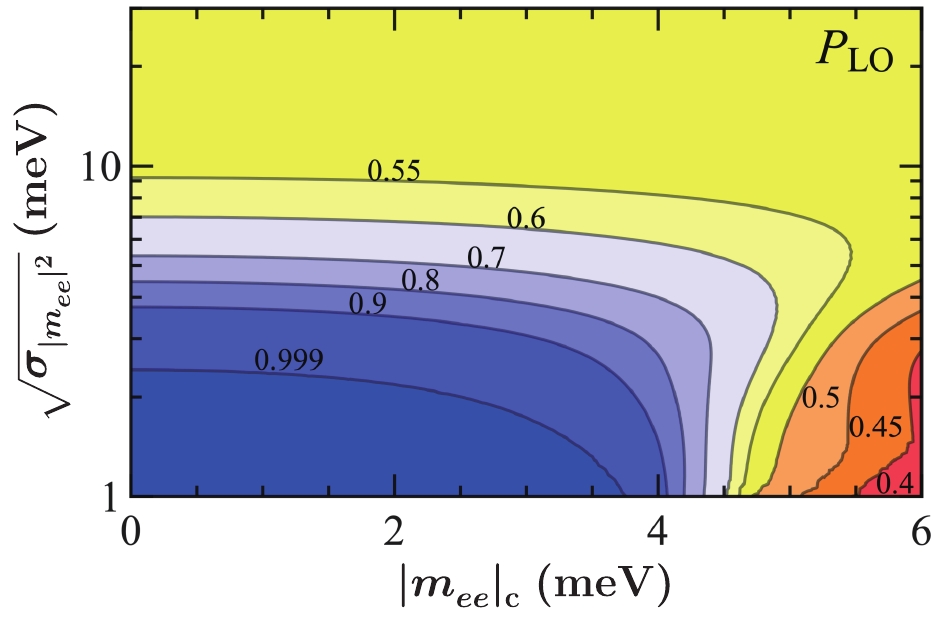

Figure 5

Figure 5.  (color online) The relative probability of NO-LO from the $0 \nu 2 \beta$ decay effective mass sensitivity ($\sigma_{|m_{ee}|^2}$) and its central value ($|m_{ee}|^2_{\rm c}$).

DownLoad: Full-Size Img PowerPoint

3. The two Majorana CP phases

• 1. Introduction
• 2. The solar octant
• 3. The two Majorana CP phases
• 4. Conclusion

If the $0 \nu 2 \beta$ decay sensitivity further improves to the sub-meV scale, it is then possible to simultaneously determine the two Majorana CP phases [19, 80, 81]. The basic logic is that the three complex vectors in Eq. (2) form a closed Majorana triangle on the complex plane if the effective mass $|m_{ee}|$ vanishes. Once the lengths $L_i$ of its three sides are known, its three inner angles can be uniquely determined as functions of $L_i$. Two of the three inner angles are actually the two Majorana CP phases as defined in Eq. (2).

Observing the $0 \nu 2 \beta$ decay indicates a nonzero effective mass $|m_{ee}|$, corresponding to only one degree of freedom. Then, only one combination of the two Majorana CP phases can be determined or constrained. But a vanishing effective mass, $|m_{ee}| = 0$, yields two independent constraints, $m_{ee} = 0$ or more explicitly, $\mathbb{R}(m_{ee}) = \mathbb{I}(m_{ee}) = 0$, where $\mathbb{R}$ and $\mathbb{I}$ extract the real and imaginary components, respectively. Two constraints can resolve two degrees of freedom, explaining why the two Majorana CP phases can be simultaneously determined. The same situation can happen for the more realistic case with some upper limit $U$, $|m_{ee}| \leqslant U$, which can convert to two independent upper limits, $\mathbb{R}(m_{ee}) \leqslant U$ and $\mathbb{I}(m_{ee}) \leqslant U$. The two Majorana CP phases are then determined/constrained within some contour. Again, the JUNO [60] and Daya Bay [63] experiments can play an important role by significantly reducing the experimental uncertainties from the oscillation parameters.

This simultaneous determination of the two Majorana CP phases can only happen when the effective mass $|m_{ee}|$ falls into the funnel region, and hence only for NO. With IO, one physical degree of freedom would become invisible forever, which is a big loss for physics search. In contrast, NO makes it possible to measure all physical variables without losing any information. No physical degrees of freedom would be missing.

It seems that the vanishing $|m_{ee}|$ is a disappointing future for the $0 \nu 2 \beta$ decay experiments, which is not necessarily true. The prospect of simultaneously determining the two Majorana CP phases provides a continuous motivation for improving the experimental sensitivity. Either we can verify the Majorana nature or measure the two Majorana CP phases. Both are physically important. To some extent, the $0 \nu 2 \beta$ decay has no-loss future. With other alternative measurements providing the Majorana nature [66–78], the $0 \nu 2 \beta$ experiment can simultaneously measure the two Majorana CP phases.

4. Conclusion

• 1. Introduction
• 2. The solar octant
• 3. The two Majorana CP phases
• 4. Conclusion

We envision the future prospect of neutrino mass ordering and its role in the $0 \nu 2 \beta$ decay by assuming the Majorana nature of neutrinos. The NO is not the seemingly boring option or "God's Mistake", but can lead to much more vivid landscapes. First, with ${\cal{O}}(10\,{\rm{meV}})$ sensitivity on the effective mass $|m_{ee}|$, the $0 \nu 2 \beta$ decay measurement can distinguish NO from IO. Second, if the sensitivity further improves to ${\cal{O}}({\rm{meV}})$, the $0 \nu 2 \beta$ decay measurement can exclude the solar HO. Different from the NO-LO option that has a funnel region in the effective mass distribution, the effective mass of the NO-HO option is bounded from below, $|m_{ee}| \geq 3.2\,(3.8)\,{\rm{meV}}$ without (with) input from JUNO. The solar angle is at the right value to separate the NO-LO region from the NO-HO one with vanishing or relatively small $m_1$. Finally, if the sensitivity improves even further to sub-meV, NO allows the two Majorana CP phases to be simultaneously determined in the absence of the $0 \nu 2 \beta$ decay signal, observing all physical degrees of freedom. During this adventure, the input of the solar angle from JUNO and the Majorana nature from independent measurements are necessary. The rich mine in the $0 \nu 2 \beta$ decay is just starting to appear, and the global fit preference of NO is not a nightmare, but an inspiring herald of a new era.

SFG would like to thank the hospitality of KIAS where this paper was partially finalized. SFG is also grateful to Danny Marfatia for bringing attention to the NSI degeneracies in the neutrino mass ordering and the solar octant.

References