-
The origin of elements in the universe is a hot topic not only in astrophysics but also in nuclear physics [1, 2]. The rapid neutron-capture process (r-process) is responsible for the production of about half of the elements heavier than iron, synthesizing elements by continuous neutron captures and
$ \beta $ decays [3-5]. The$ \beta $ decay governs the r-process matter flow between neighboring isotopic chains, and hence sets the time scale of the r-process. Therefore,$ \beta $ decay is a key process in r-process nucleosynthesis, and has been the focus of much attention in recent r-process studies [6-9].There are some potential candidates for r-process sites, which can provide the conditions of high neutron density and high temperature, such as the neutrino-driven wind after the formation of a proto-neutron star in core collapse supernovae [10-12] and neutron star mergers [13, 14]. However, the r-process sites have still not been fully determined, partly due to the uncertainties in its nuclear physics inputs, including nuclear
$ \beta $ -decay half-lives and neutron-capture rates [15]. Therefore, it is essential to obtain accurate nuclear$ \beta $ -decay half-lives from theoretical and experimental studies. Although the measurements of$ \beta $ -decay half-lives have made great progress in recent years [16, 17], many neutron-rich nuclei related to the r-process still cannot be reached by present or even next-generation experimental facilities, so theoretical predictions are essential to r-process simulations. Many approaches have been developed to study nuclear$ \beta $ -decay half-lives, including the gross theory [18-20] and the shell model [21]. Moreover, quasiparticle random-phase approximation (QRPA) approaches based on the finite-range droplet model (FRDM) [22-24], density functional theory (DFT) [25-27], and covariant DFT [28-32] have also been widely employed to predict nuclear$ \beta $ -decay half-lives. In addition, the QRPA with particle-vibration coupling has also been applied to the predictions of nuclear$ \beta $ -decay half-lives [33, 34]. However, there are large variations among these half-life predictions with different approaches. Therefore, it is necessary to investigate the uncertainties in theoretical predictions of nuclear$ \beta $ -decay half-lives.The shell model is only feasible for light nuclei or nuclei near the magic numbers, due to the limitation of configuration spaces. Although the QRPA approach can in principle be applied to arbitrary heavy systems, it is still very time consuming when making systematic calculations for deformed systems. Recently, an empirical formula based on the Fermi theory has been proposed to predict the nuclear
$ \beta $ -decay half-lives [35]. The parameters in this empirical formula can be obtained by fitting to the known half-lives, and it can even deal with both shell and pairing effects, so it can describe nuclear$ \beta $ -decay half-lives with a high accuracy approaching that of machine learning calculations [36]. This gives us the confidence to predict the half-lives of unknown neutron-rich nuclei with this empirical formula. The$ \beta $ -decay energy is a key input for this empirical formula, in addition to the proton number Z and neutron number N. However, the decay energies predicted by different nuclear mass models are very different, which can certainly induce the variations in the half-life predictions.In this work, we will investigate the uncertainties of nuclear
$ \beta $ -decay half-life predictions with this empirical formula by employing ten nuclear mass models. These include two microscopic mass models (the relativistic mean field (RMF) [37] and the Hartree-Fock-Bogoliubov (HFB-31) [38]), five macroscopic-microscopic mass models (the extended Thomas-Fermi plus Strutinsky integral (ETFSI-Q) [39], ETFSI-2 [40], the Koura-Tachibana-Uno-Yamada (KTUY) [41], FRDM12 [42] and the Weizsäcker-Skyrme (WS4) [43]), one macroscopic mass model (the Bethe and von Weizsäcker (BW2) [44]), and two other global mass models (Bhagwat [45] and DZ28 [46]). These nuclear mass models can provide reasonable estimates of nuclear masses, while the accuracy of their mass predictions can be further improved by the radial basis function (RBF) approach [47-49], the RBF approach with odd-even effects [50-52], and the Bayesian neural network (BNN) approach [53-56]. Therefore, it is interesting to explore the uncertainties of half-life predictions with this empirical formula. Special attention is focused on the theoretical uncertainties from nuclear$ \beta $ -decay energies and the parameters of the empirical formula. The corresponding results and discussion are presented in Section III. The basic formula employed in this work will be given in Section II, and a summary will be presented in Section IV. -
The nuclear
$ \beta $ -decay half-life can be described with the well-known Fermi theory [57], where the phase-space factor is complicated and should be calculated with a numerical method. The emitted electron from$ \beta $ decay of a neutron-rich nucleus generally has a very large speed, and hence the phase-space factor in the Fermi theory can be approximated with the extreme-relativistic limit [35]. With the corrections from pairing and shell effects, the nuclear$ \beta $ -decay half-life$ T_{1/2} $ can be predicted with the following empirical formula [35]$ \begin{aligned}[b] \log T_{1/2} = & a_{6}+\left({\alpha}^{2}Z^{2}-5-a_{7}\frac{N-Z}{A}\right)\log(Q-a_{8}\delta) \\ &+a_{9}{\alpha}^{2}Z^{2}+\frac{1}{3}{\alpha}^{2}Z^{2}\log A-{\alpha} Z\pi+S(Z,N),\; \; \; \; \end{aligned} $

(1) where
$ \alpha = 1/137 $ is the fine structure constant,$ A = Z+N $ is the mass number, and$ \delta = (-1)^{N}+(-1)^{Z} $ is a quantity related to the nuclear pairing effect. The last term$ S(Z,N) $ is introduced to describe the shell effect in nuclear$ \beta $ -decay half-lives, which is:$ \begin{aligned}[b] S(Z,N) =& a_{1}{\rm{e}}^{-\left((N-28)^{2}+(Z-20)^{2}\right)/12} \\ &+ a_{2}{\rm{e}}^{-\left((N-50)^{2}+(Z-38)^{2}\right)/43} \\ &+ a_{3}{\rm{e}}^{-\left((N-82)^{2}+(Z-50)^{2}\right)/13} \\ &+ a_{4}{\rm{e}}^{-\left((N-82)^{2}+(Z-58)^{2}\right)/24} \\ &+ a_{5}{\rm{e}}^{-\left((N-110)^{2}+(Z-70)^{2}\right)/244}. \end{aligned} $

(2) Q in Eq. (1) is the
$ \beta $ -decay energy, which can be determined from mass predictions of nuclear models. The nine parameters$ a_i\; (i = 1,\; 2,\; ...,\; 9) $ in Eqs. (1) and (2) are optimized from a least squares fit to the experimental half-lives with the Levenberg-Marquardt method. The experimental half-lives are taken from NUBASE2016 [16], and only those nuclei with$ Z,\; N\geqslant 8 $ and$ T{_{1/2}}\leqslant 10^6 $ s are retained. To study the influence of these parameters on half-life predictions, they are determined with three different data sets, i.e. those sets for nuclei with half-lives shorter than$ 10^{6} $ ,$ 10^{3} $ , and 1 s, which are denoted by$ T_{1/2}^{\rm S6},\; T_{1/2}^{\rm S3} $ , and$ T_{1/2}^{\rm S0} $ for simplicity hereafter. There are$ 1009 $ ,$ 824 $ , and$ 381 $ experimental half-lives in the data sets for$ T_{1/2}^{\rm S6},\; T_{1/2}^{\rm S3} $ , and$ T_{1/2}^{\rm S0} $ , respectively.In order to evaluate the performance of this empirical formula with Q values for different mass models, the root-mean-square (rms) deviation of the logarithms of the calculated half-lives
$ T_{1/2}^{\rm{cal}} $ with respect to that of the experimental data$ T_{1/2}^{\exp} $ is employed in the following$ {\sigma _{{\rm{rms}}}}({\log _{10}}{T_{1/2}}) = \sqrt {\dfrac{1}{n}\displaystyle\sum\limits_{i = 1}^n {\left[ {{{\log }_{10}}\left( {\dfrac{{T_{1/2}^{{\rm{cal}}}}}{{T_{1/2}^{\exp }}}} \right)} \right]_i^2} } . $

(3) Here, n is the number of nuclei in a given data set from NUBASE2016 [16]. For each nucleus, the theoretical uncertainties of this empirical formula from different Q predictions are estimated with the following rms quantity:
$ {\delta _{{\rm{rms}}}}({\log _{10}}{T_{1/2}}) = \sqrt {\dfrac{1}{{m - 1}}\displaystyle\sum\limits_{j = 1}^m {\left[ {{{\log }_{10}}\left( {\dfrac{{T_{1/2}^{{\rm{cal}}}}}{{T_{1/2}^{{\rm{aver}}}}}} \right)} \right]_j^2} } ,$

(4) where
$ T_{1/2}^{\rm{aver}} $ is the average value of$ T_{1/2}^{\rm{cal}} $ from the different mass models. m is the number of nuclear mass models, which are used to determine Q values. To get a reasonable estimation of uncertainty, we only calculate$ \delta_{\rm{rms}}(\log_{10} T_{1/2}) $ for those nuclei whose Q values can be obtained by at least$ 6 $ mass models. -
We study the accuracy of the empirical formula for different nuclei with different half-lives. The rms deviations
$ \sigma _{\rm{rms}}(\log_{10} T_{1/2}) $ defined in Eq. (3) are shown in Table 1 for various nuclear mass models. It is clear that this formula can reproduce the known half-lives$ T_{1/2}<10^6 $ s within one order of magnitude for all mass models considered here. The BW2 and WS4 models give the largest and smallest$ \sigma_{\rm{rms}}(\log_{10} T_{1/2}) $ , which are$ 0.94 $ and$ 0.66 $ , respectively. This accuracy is similar to, and even better than, that obtained by the QRPA approach based on FRDM [23], whose$ \sigma_{\rm{rms}}(\log_{10} T_{1/2}) = 0.82 $ . It is also found that$ \sigma_{\rm{rms}}(\log_{10} T_{1/2}) $ gradually decreases for the nuclear sets with shorter half-lives, which indicates that this formula better reproduces the experimental data of nuclei with shorter half-lives. The best accuracy is achieved with the WS4 mass prediction, whose$\sigma_{\rm{rms}}(\log_{10} T_{1/2}) = 0.22$ for the nuclear set with$ T_{1/2}<1 $ s, i.e. it can reproduce the experimental half-lives within about a factor of 2.Model $ \sigma_{\rm{rms}}(\log_{10}T^{\rm S6}_{1/2}) $ 

$ \sigma_{\rm{rms}}(\log_{10}T^{\rm S3}_{1/2}) $ 

$ \sigma_{\rm{rms}}(\log_{10}T^{\rm S0}_{1/2}) $ 

Bhagwat 0.69 0.41 0.24 BW2 0.94 0.58 0.30 DZ28 0.74 0.42 0.23 ETFSI-2 0.73 0.45 0.23 ETFSI-Q 0.79 0.57 0.26 FRDM2012 0.72 0.44 0.25 HFB-31 0.81 0.51 0.27 KTUY 0.67 0.43 0.26 RMF 0.83 0.55 0.30 WS4 0.66 0.39 0.22 Table 1. The rms deviations
$ \sigma _{\rm{rms}}(\log_{10} T_{1/2}) $ of nuclear$ \beta $ -decay half-lives with respect to the experimental data for various nuclear mass models. The rms deviations for$ T^{\rm S6} $ ,$ T^{\rm S3} $ , and$ T^{\rm S0} $ are calculated with respect to the experimental data of nuclear sets with$ T_{1/2}<10^6 $ s,$ T_{1/2}<10^3 $ s, and$ T_{1/2}<1 $ s, respectively.To check the extrapolation ability of the empirical formula,
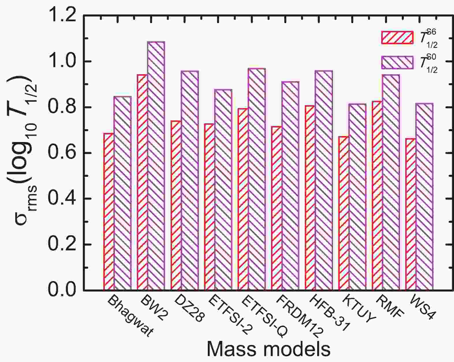
$ \sigma _{\rm{rms}}(\log_{10} T_{1/2}) $ of$ T_{1/2}^{\rm S0} $ for the nuclear set with$ T_{1/2}<10^6 $ s are shown by the right-hand bars in Fig. 1. For comparison, the corresponding results for$ T_{1/2}^{\rm S6} $ are shown by the left-hand bars in Fig. 1. Since the known half-lives with$ 1\; {\rm{s}}<T_{1/2}<10^6\; {\rm{s}} $ are not the fitting data of$ T_{1/2}^{\rm S0} $ , it is found that the accuracies of$ T_{1/2}^{\rm S0} $ are worse than those of$ T_{1/2}^{\rm S6} $ for the nuclear set with$ T_{1/2}<10^6 $ s. However, they are still reasonable, with$ \sigma _{\rm{rms}}(\log_{10} T_{1/2}) $ between$ 0.81 $ and$ 1.08 $ for various nuclear mass models. This indicates that the empirical formula has reliable extrapolation ability even for long-lived nuclei, whose half-lives are generally difficult to describe with microscopic nuclear models.
Figure 1. (color online) The rms deviations
$ \sigma _{\rm{rms}}(\log_{10} T_{1/2}) $ for the nuclear set with$ T_{1/2}<10^6 $ s. For each nuclear model, the left- and right-hand bars correspond to the results for$ T_{1/2}^{\rm S6} $ and$ T_{1/2}^{\rm S0} $ , respectively.As in Fig. 1, we show
$ \sigma _{\rm{rms}}(\log_{10} T_{1/2}) $ of$ T_{1/2}^{\rm S6} $ for the nuclear set with$ T_{1/2}<1 $ s in Fig. 2, and the corresponding results for$ T_{1/2}^{\rm S0} $ are also shown for comparison. Clearly,$ T_{1/2}^{\rm S6} $ still reproduces the experimental data better for the short-lived nuclei, whose$ \sigma _{\rm{rms}}(\log_{10} T_{1/2}) $ for the nuclear set with$ T_{1/2}<1 $ s is only about half of its value for nuclear set with$ T_{1/2}<10^6 $ s. The accuracy of$ T_{1/2}^{\rm S6} $ is slightly larger than that of$ T_{1/2}^{\rm S0} $ , but it is still reasonable to make half-life predictions. For example, the accuracy of$ T_{1/2}^{\rm S6} $ for the WS4 model is similar to those of the$ T_{1/2}^{\rm S0} $ for BW2 and RMF models. Therefore, both$ T_{1/2}^{\rm S6} $ and$ T_{1/2}^{\rm S0} $ will be used to evaluate the uncertainties of half-lives for those unknown neutron-rich nuclei in the following, and their differences are employed to describe the uncertainties of half-life predictions from the parameters of the empirical formula.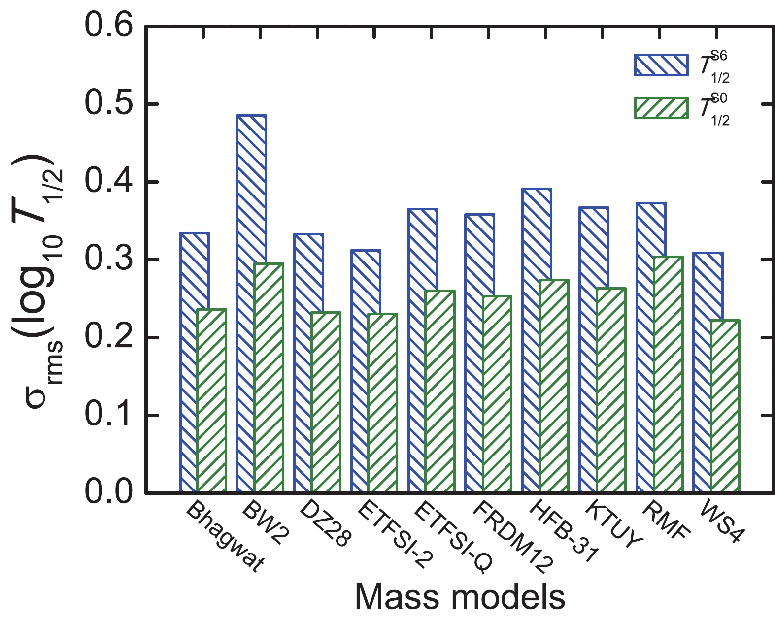
Figure 2. (color online) Same as Fig. 1, but the rms deviations
$ \sigma _{\rm{rms}}(\log_{10} T_{1/2}) $ are for the nuclear set with$ T_{1/2}<1 $ s.To investigate the predictive ability of the empirical formula in detail, we show the predicted
$ \beta $ -decay half-lives of the$ N = 50,\; 82 $ , and$ 126 $ isotones with$ T_{1/2}^{\rm S6} $ and$ T_{1/2}^{\rm S0} $ in Fig. 3. Clearly, the empirical formula reproduces the experimental data well for both$ T_{1/2}^{\rm S6} $ and$ T_{1/2}^{\rm S0} $ .$ T_{1/2}^{\rm S6} $ predicts longer half-lives than$ T_{1/2}^{\rm S0} $ for nuclei with$ T_{1/2} \gtrsim 0.01 $ s, and shorter half-lives than$ T_{1/2}^{\rm S0} $ for nuclei with$ T_{1/2} \lesssim 0.01 $ s, while they predict similar half-lives for nuclei with$ T_{1/2}\sim 0.01 $ s. Furthermore, it is found that the uncertainties in the half-lives are relatively large for$ N = 50 $ and$ 82 $ isotones with$ T_{1/2} \lesssim 0.01 $ s and$ T_{1/2} \gtrsim 1 $ s, while the uncertainties remain large for all$ N = 126 $ isotones shown here. The large uncertainties can be understood from the sensitivity of$ T_{1/2} $ to the Q value and the large uncertainties of the Q values. For the long-lived nuclei, their Q values are so small that tiny differences in Q values would induce large uncertainties in the half-life predictions. For the short-lived nuclei, the uncertainties in the Q values become large since they are far from the known region, which leads to the large uncertainties in the half-lives. For$ N = 126 $ isotones, only a few long-lived nuclei are known, so the uncertainties in the Q values are always large for the unknown nuclei and hence induce the large uncertainties in the half-lives. In addition, it should be pointed out that the uncertainties for the r-path nuclei at$ N = 126 $ are about one order of magnitude, which is relatively larger than those for r-path nuclei at$ N = 50 $ and$ 82 $ . Therefore, future experiments on r-process-path nuclei around$ N = 126 $ would help to reduce the uncertainties in their half-lives and further improve our understanding of the r-process. Similar to Fig. 3, the half-lives of$ Z = 28,\; 50 $ , and$ 82 $ isotopes are shown in Fig. 4. The conclusion found in Fig. 3 is also valid for the$ Z = 28,\; 50 $ , and$ 82 $ isotopes, which further testify to the reliability of the empirical formula to study nuclear$ \beta $ -decay half-lives.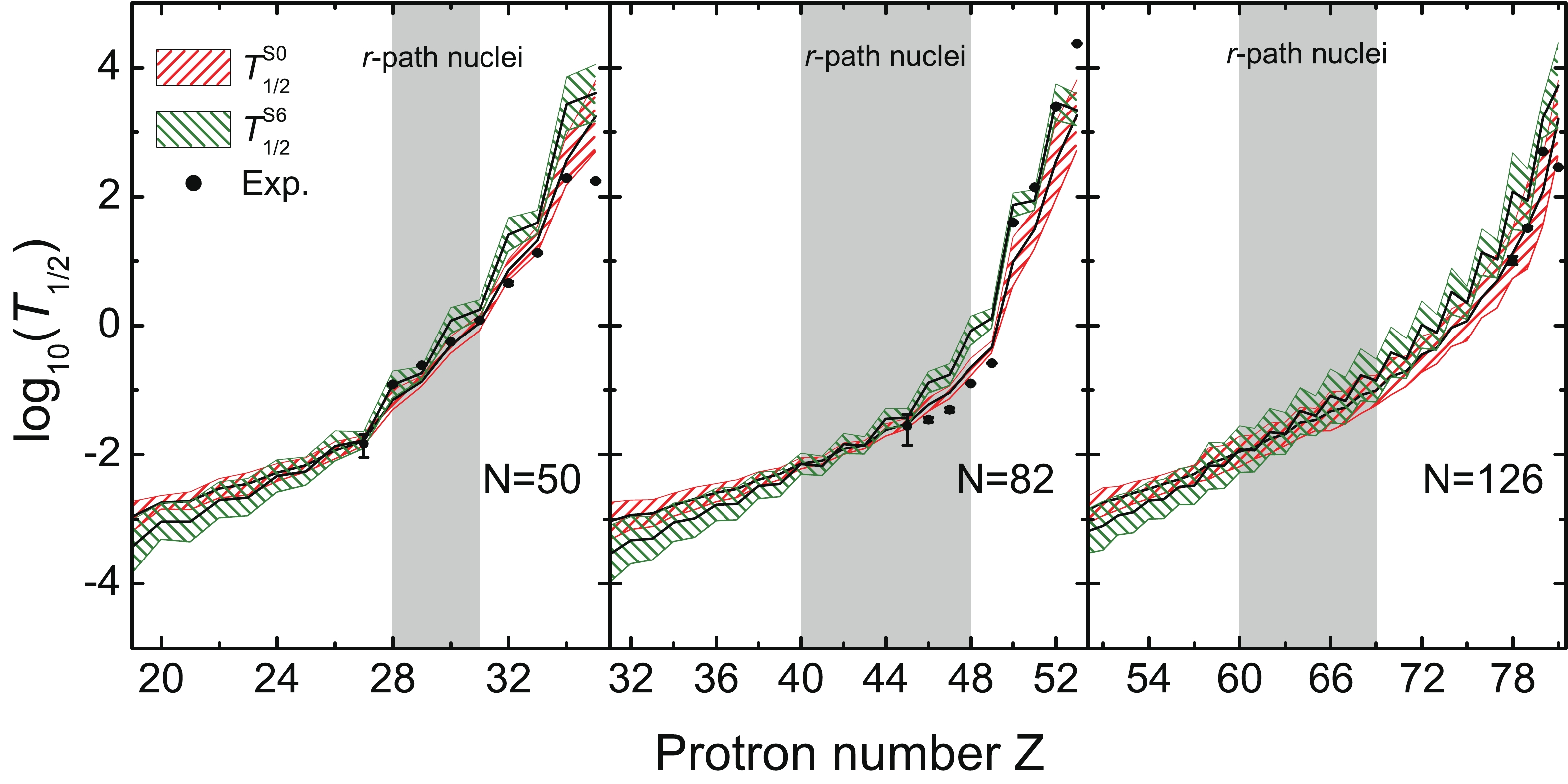
Figure 3. (color online) The logarithm of nuclear
$ \beta $ -decay half-lives for$ N = 50, \;82,\;126 $ isotones. The red-hatched and olive-hatched bands correspond to the error bands of$ T_{1/2}^{\rm S0} $ and$ T_{1/2}^{\rm S6} $ , respectively, which are evaluated with$ \sigma _{\rm{rms}}(\log_{10} T_{1/2}) $ in Eq. (3). For comparison, the experimental half-lives are shown by the filled circles.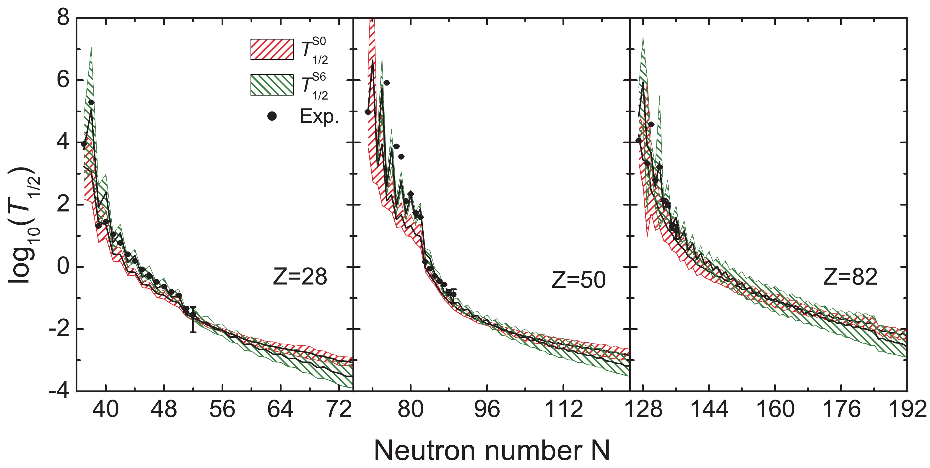
Figure 4. (color online) Same as Fig. 3, but for
$ Z = 28,\; 50 $ , and$ 82 $ isotopes.In order to systematically study the theoretical uncertainties in the calculation of nuclear
$ \beta $ -decay half-lives with the empirical formula, the rms deviations$ \delta_{\rm{rms}}(\log_{10} T_{1/2}) $ defined in Eq. (4) for$ T_{1/2}^{\rm S0} $ and$ T_{1/2}^{\rm S6} $ are shown in Fig. 5(a) and (b), respectively. Clearly, the uncertainties in the$ \beta $ -decay half-lives from nuclear mass uncertainties for$ T_{1/2}^{\rm S0} $ are generally smaller than those for$ T_{1/2}^{\rm S6} $ . The heavy nuclei and the nuclei near the neutron-drip line are generally far away from the known region, so different models usually predict very different nuclear masses and hence lead to large uncertainties in the$ \beta $ -decay energies. From Eq. (1), it is clear that the nuclear$ \beta $ -decay half-lives are very sensitive to decay energies, so the uncertainties in the half-lives would be relatively larger for the heavy nuclei and the nuclei near the neutron-drip line, which is also clearly shown in Fig. 5. For the nuclei around$ Z = 70 $ and$ N = 160 $ , their$ \beta $ -decay energies suddenly drop from about 20 MeV to about 5 MeV for the ETFSI-Q model. However, they remain about 20 MeV for all other models considered here. This sudden drop of decay energy leads to the sudden increase of half-lives in the ETFSI-Q model. Therefore, the predicted half-lives from the ETFSI-Q model are very different from those of other models for these nuclei, which further leads to large uncertainty around$ Z = 70 $ and$ N = 160 $ in both subfigures of Fig. 5.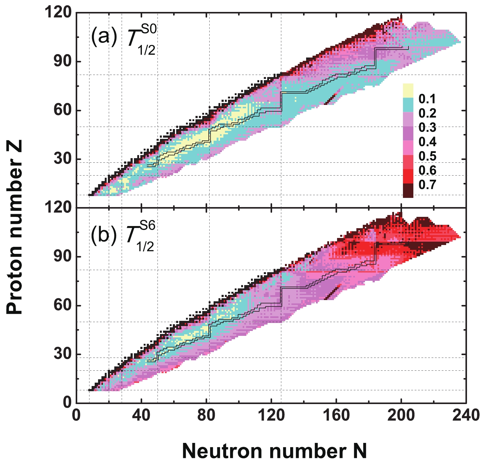
Figure 5. (color online) Uncertainties of nuclear
$ \beta $ -decay half-lives$ \delta_{\rm{rms}}(\log_{10} T_{1/2}) $ for$ T_{1/2}^{\rm S0} $ and$ T_{1/2}^{\rm S6} $ . To guide the eye, the r-process path calculated with the RMF mass model [37] and the stable nuclei are shown by the black lines and black filled squares, respectively.The differences in the average values of
$ \beta $ -decay half-lives between$ T_{1/2}^{\rm S0} $ and$ T_{1/2}^{\rm S6} $ are shown in Fig. 6. A remarkable odd-even staggering is found for the differences in$ \beta $ -decay half-lives, and the differences for the even-even nuclei are generally larger than the odd-odd nuclei. This implies the importance of pairing correlation on the accurate predictions of$ \beta $ -decay half-lives. It is interesting to find that the differences in$ \beta $ -decay half-lives are generally smaller for nuclei around the r-process path, so it would be relatively reliable to make r-process calculations using the$ \beta $ -decay half-life predictions of this empirical formula. The data table for the$ \beta $ -decay half-life predicted in this work is available at xsx.ahu.edu.cn/T12Data.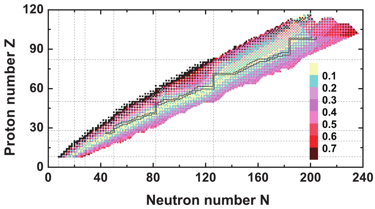
Figure 6. (color online) Same as Fig. 5, but for the differences in the average values of
$ \beta $ -decay half-lives between$ T_{1/2}^{\rm S0} $ and$ T_{1/2}^{\rm S6} $ . -
In this work, the uncertainties in theoretical predictions of nuclear
$ \beta $ -decay half-lives have been explored with the latest empirical formula. Special attention is focused on the theoretical uncertainties from nuclear$ \beta $ -decay energies and the parameters of the empirical formula. It is found that the uncertainties in the half-lives are relatively large for heavy nuclei and nuclei near the neutron-drip line. For the nuclei on the r-process path, the uncertainties for those with$ N = 126 $ are about one order of magnitude, which is considerably larger than those with$ N = 50 $ and$ 82 $ . The parameters in the empirical formula were determined for three different data sets with half-lives shorter than$ 10^{6} $ ,$ 10^{3} $ , and 1 s, with the resulting empirical formulas denoted$ T_{1/2}^{\rm S6} $ ,$ T_{1/2}^{\rm S3} $ , and$ T_{1/2}^{\rm S0} $ , respectively. The differences between the predictions of$ T_{1/2}^{\rm S6} $ and$ T_{1/2}^{\rm S0} $ were employed to describe the uncertainties in the half-life predictions from the parameters of the empirical formula. The empirical formula reproduces the experimental data well for both$ T_{1/2}^{\rm S6} $ and$ T_{1/2}^{\rm S0} $ , especially for those short-lived nuclei with$ T_{1/2}< 1 $ s.$ T_{1/2}^{\rm S6} $ predicts longer half-lives than$ T_{1/2}^{\rm S0} $ for nuclei with$ T_{1/2} \gtrsim 0.01 $ s and shorter half-lives than$ T_{1/2}^{\rm S0} $ for nuclei with$ T_{1/2} \lesssim 0.01 $ s, while they predict similar half-lives for nuclei with$ T_{1/2}\sim 0.01 $ s. Since the half-lives of nuclei on the r-process path are typically around$ 0.01 $ s, the uncertainties from the parameters of the empirical formula are relatively small for these r-path nuclei. This indicates that the empirical formula is very suitable for$ \beta $ -decay half-life predictions in r-process simulations. -
We would like to express our gratitude to N. N. Zhou, B. R. Yu, and Z. B. Pei for fruitful discussions.
Exploring the uncertainties in theoretical predictions of nuclear β-decay half-lives
- Received Date: 2020-10-14
- Available Online: 2021-04-15
Abstract: Nuclear


 Abstract
 HTML
HTML Reference
 Related
 PDF
PDF




 DownLoad: