Cosmological implications of a B − L charged hidden scalar: leptogenesis and gravitational waves

Since the discovery of the standard model (SM) Higgs at the Large Hadron Collider (LHC), understanding the hierarchy problem has become one of the most challenging theoretical difficulties in the SM. In light of null results in searches of new physics at the LHC, in particular the supersymmetric particles, concern on the hierarchy problem is increasing. This is also intimately related to the spontaneous electroweak symmetry breaking (EWSB), which is responsible for the generation of SM particle masses, and might imply more fundamental theories at a higher energy scale. One elegant solution is the Coleman-Weinberg mechanism [1], in which the original potential is classically conformal and EWSB is induced when the mass term is generated radiatively. As the conformal invariant version of the SM is not consistent with the Higgs data, the Higgs portal interaction and an extra singlet scalar Φ can be used to obtain a natural EWSB [2, 3]. Recently, the conformal $U(1)_{B-L}$ model has raised great interests as this model can naturally accommodate tiny neutrino masses via the type-I seesaw mechanism [4-8]. Furthermore, lepton asymmetry can be generated through the leptogenesis mechanism [9], which is then transferred to baryon asymmetry through the electroweak sphaleron process. Some relevant recent studies are reported in Refs. [10, 11].

The breaking of $U(1)_{B-L}$ symmetry can occur through phase transition as the Universe cools. Afterward, gravitational waves (GWs) might be emitted from cosmic strings [12-14]. If the phase transition is of first order, GWs could be generated and probed through future GW experiments [15-23], such as LISA [24, 25], Taiji [26], TianQin [27], Big Bang Observer (BBO) [28], DECi-hertz Interferometer Gravitational wave Observatory (DECIGO) [29], and Ultimate-DECIGO [30]. It has been found that a complex scalar charged under the $U(1)_{B-L}$ symmetry can trigger a first-order phase transition within the conformal framework [31].

In this study, we investigated the impact of a hidden complex singlet scalar ${\cal{S}}$ on leptogenesis and GWs in the conformal $U(1)_{B-L}$ model, with ${\cal{S}}$ charge $n_{\cal{S}}$ under the $U(1)_{B-L}$ symmetry (see Table 1). For the sake of concreteness, we considered the TeV-scale resonant leptogenesis with two mass quasi-degenerate right-handed neutrinos (RHNs) [32-35]. The heavy RHNs couple to the conformal scalar Φ and the heavy $Z'$ gauge boson from the $U(1)_{B-L}$ symmetry breaking, and the processes $NN \to$$f\bar{f},\, \Phi\Phi,\, \Phi Z'$ (where f represents SM fermions) will dilute the heavy RHNs by two units, thus potentially reducing the lepton and baryon asymmetry significantly [36-41]. For our study, the leptogenesis diffusion process was found to be further disturbed by the annihilation process $NN \to {\cal{S}} {\cal{S}}^\dagger$ due to the $B-L$ charge of ${\cal{S}}$ (see the diagrams in Fig. 2). It is found that this extra dilution effect of ${\cal{S}}$ falsifies leptogenesis in a large region of parameter space (see Fig. 3). The hidden scalar ${\cal{S}}$ can also play an important role in the phase transition and GW emission; see examples in Fig. 4. For appropriate charges $n_{\cal{S}}$, ${\cal{S}}$ can be stabilized by the accidental $B-L$ symmetry, and thus play the role of dark matter (DM). However, the stringent limits from the DM direct detection experiments, LUX [42], PandaX-II [43, 44] and Xenon1T [45], have ruled out the possibility of ${\cal{S}}$ as WIMP DM with the observed relic density within the framework under study [46-48]. Therefore, we refer to ${\cal{S}}$ as a “hidden” scalar throughout this paper.

	SU(3)c	SU(2)L	U(1)Y	U(1)B−L
$q_{L}^i$	3	2	+1/6	+1/3
$u_R^i$	3	1	+2/3	+1/3
$d_R^i$	3	1	−1/3	+1/3
$\ell^i_L$	1	2	−1/2	−1
$N_i$	1	1	0	−1
$e_R^i$	1	1	−1	−1
H	1	2	+1/2	0
Φ	1	1	0	+2
${\cal{S}}$	1	1	0	$n_{\cal{S}}$

Table 1.  Particle content of the conformal $U(1)_{B-L}$ model: In addition to the SM particles, there are three RHNs $N_i$ ($i=1,2,3$), a complex singlet scalar Φ, and another complex singlet scalar ${\cal{S}}$.

The rest of this paper is organized as follows: In Section II, we introduce the conformal $U(1)_{B-L}$ extension of the SM with the hidden scalar ${\cal{S}}$. The current LHC constraints on the $Z'$ boson and the collider search prospect of ${\cal{S}}$ are also explored. The impact of ${\cal{S}}$ on resonant leptogenesis is studied in Section III. The cosmological symmetry breaking history and the GWs generated during phase transition are investigated in Section IV, and then, we conclude the study in Section V. The renormalization group equations (RGEs) of the conformal $U(1)_{B-L}$ model are presented in Appendix A, the theoretical constraints of stability and perturbativity are discussed in Appendix B, and the reduced cross sections for leptogenesis are provided in Appendix C.

The particle content of the conformal $U(1)_{B-L}$ model is presented in Table 1, where $q_L$, $u_R$ and $d_R$ are respectively the SM quark doublets and singlets, $\ell_L$ and $e_R$ are the SM lepton doublets and singlets, and H is the SM-like Higgs doublet. Three RHNs $N_i$, two complex singlet scalars Φ, and ${\cal{S}}$ are introduced to the model. To implement EWSB, the most general scalar potential for the fields H, Φ, and ${\cal{S}}$ reads

with

For simplicity, all the coupling coefficients in potential (1) are assumed to be positive, which ensures that no vacuum expectation value (VEV) is generated for ${\cal{S}}$. The hidden scalar ${\cal{S}}$ can be stabilized by the accidental $B-L$ symmetry [48] when its $B-L$ charge $n_{\cal{S}} \neq \pm2 n$ with the positive integer $n\leqslant 4$. The Yukawa interactions are given below:

where we do not show explicitly the flavor indices for the sake of clarity, and C is the charge conjugate operator. The 1-loop Coleman-Weinberg potential of the scalar field Φ triggers the breakdown of the $B-L$ symmetry. With the scalar field $\Phi = \phi/\sqrt{2}$, the Coleman-Weinberg potential can be calculated using [1]

where the couplings $\lambda_\phi$ and $\lambda_P$ depend on the energy scale µ, and the exact expression for the β-function $\beta_{\lambda_\phi}$ is given in Eq. (A3). The potential in Eq. (4) leads to the $B-L$ symmetry breaking with $\langle \Phi \rangle = v_{BL}/\sqrt2$. After this, tiny neutrino masses are generated through the type-I seesaw mechanism $m_\nu = - Y_D {\cal{M}}_N^{-1} Y_D^{\sf T} v_{\rm{EW}}^2/2$, with ${\cal{M}}_N =$$Y_\phi v_{BL}/\sqrt2$, the RHN mass matrix. The mass for the $U(1)_{B-L}$ gauge boson $Z'$ is given by

where $g_{BL}$ is the gauge coupling for the $U(1)_{B-L}$ gauge group. The mass for the ${\cal{S}}$ field is

The mass of the ϕ field can be expressed as

One can see from Eq. (7) that the spontaneous symmetry breaking of the $U(1)_{B-L}$ symmetry requires $4 m_{S}^4+6 m_{Z'}^4 \gtrsim m_N^4$. Assuming $Y_\phi$ is much smaller than $g_{BL}$ and $\lambda_{\phi S}$, which implies that the RHNs are much lighter than the $v_{BL}$ scale, we have

If both the contributions of $\lambda_{\phi S}$ and $Y_\phi$ to $\beta_{\lambda_\phi}$ are negligible in Eq. (A3), the above relation reduces to

After the breaking of $B-L$ symmetry, a non-vanishing VEV of Φ generates a mass parameter $\mu_H^2 = - \dfrac12 \lambda_{\rm{P}} v_{BL}^2$ for the doublet H in the potential of Eq. (2), which induces the spontaneous EWSB. The $U(1)_{B-L}$ breaking scale $v_{BL}$ and the SM-like Higgs VEV $v_{\rm{EW}}$ are related through the following:

Here, for the sake of simplicity, we assumed that the quartic coupling $\lambda_{HS}$ is sufficiently small such that the electroweak contribution to the hidden scalar mass $m_{\cal{S}}$ is negligible.

Before proceeding to the next subsection, we express the explicit coupling of $Z'$ to RHNs, which turns out to be

and it plays an important role in resonant leptogenesis in Section III.

For a TeV-scale $v_{BL}$, the $Z'$ mass is stringently constrained by the dilepton data $pp \to Z' \to \ell^+ \ell^-$ (with $\ell =$$e,\, \mu$) at the LHC [49, 50]. For a sequential $Z'$ boson with the same couplings as in the SM, the current ATLAS and CMS 13 TeV data requires that $m_{Z'} > 4.05$ TeV at the 95% confidence level [51, 52]. The production cross section $\sigma (pp \to Z' \to \ell^+ \ell^-)$ in the $U(1)_{B-L}$ model can be obtained by rescaling that of a sequential heavy $Z'$ boson, as a function of the gauge coupling $g_{BL}$ [53]. Accordingly, the partial decay widths of the $Z'$ boson into the SM fermions, the heavy RHNs, and the hidden scalar ${\cal{S}}$ are respectively given as

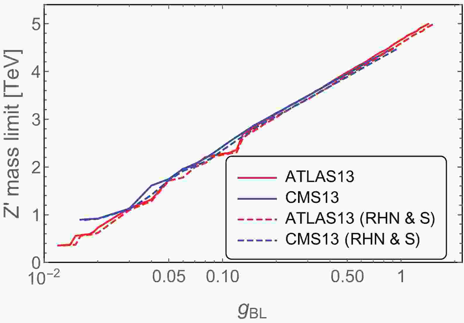
where $N_C$ is the color factor (3 for quarks and 1 otherwise); $B_f$ and $L_f$ are the baryon and lepton numbers for the SM fermions, respectively; and $S_f$ is the symmetry factor (1 for the quarks and charged leptons and $1/2$ for the light neutrinos). All these decay modes are universally proportional to $g_{BL}$. In the absence of the heavy RHNs and the ${\cal{S}}$ field, the branching fraction ${\rm{BR}} (Z' \to \ell^+ \ell^-)$ is a constant, being $8/23$, in the limit of $m_{Z'} \gg m_f$, and the production cross section $\sigma (pp \to Z') \propto g_{BL}^2$. As a result, when $g_{BL}$ increases, the dilepton limits on the $Z'$ mass tend to be stronger (See also Ref. [54] for the latest LHC bounds on the $B-L$ $Z'$ mass from Run-2 data). The constraints from the ATLAS [51] and CMS [52] 13 TeV data are shown respectively as the solid red and blue curves in Fig. 1. As a comparison, the dilepton limits on $Z'$ mass in the presence of the three RHNs and ${\cal{S}}$ are also shown by the dashed curves, assuming their masses are significantly lower than $m_{Z'}/2$; thus, the decays $Z' \to NN,\, {\cal{S}} {\cal{S}}^\dagger$ are kinematically allowed. As a result of these extra decays modes, the dilepton limits in Fig. 1 are slightly weaker. For illustration purpose, we adopted three different benchmark values of $g_{BL} = 0.1$, $0.3$, and $1.0$, interpreted the solid lines in Fig. 1, and obtained the current dilepton constraints on the $Z'$ boson mass and the corresponding limits on $v_{BL}$, which are presented in Table 2. At the high-luminosity LHC (HL-LHC) and future 100 TeV colliders, the prospects of the $Z'$ boson could be largely improved [55-57].

Figure 1.  (color online) Dilepton limits on the $Z'$ boson mass from the 13 TeV data by ATLAS [51] (red) and CMS [52] (blue), as a function of the gauge coupling $g_{BL}$. The solid curves assume that the $Z'$ boson decays only into the SM fermions, while for the dashed curves, $Z'$ decays also into the three RHNs and hidden scalar ${\cal{S}}$.

gBL	without RHNs & ${\cal S}$			with RHNs & ${\cal S}$
	$m_{Z'}$/TeV	$v_{BL}$/TeV		$m_{Z'}$/TeV	$v_{BL}$/TeV
0.1	2.42	17.2		2.35	16.6
0.3	3.49	8.22		3.43	8.08
1.0	4.66	3.30		4.59	3.25

Table 2.  Lower bounds on the $Z'$ boson mass $m_{Z'}$ and the corresponding lower limits on the $v_{BL}$ scale in the $U(1)_{B-L}$ model from the current LHC13 data [51, 52] (cf. Fig. 1).

The hidden scalar ${\cal{S}}$ can be produced at high-energy colliders in the scalar portal or the gauge portal. In the scalar portal, ${\cal{S}}$ and ${\cal{S}}^\dagger$ can be pair produced through both the SM Higgs h and the scalar ϕ, assisted by the $h - \phi$ mixing, which is induced by the $\lambda_P$ term in the potential (2). In particular, the most important production channel is from the gluon-fusion production of SM Higgs h or ϕ, associated with a gluon jet emitted from the initial partons, i.e.,

The hidden scalar particles ${\cal{S}}$ and ${\cal{S}}^\dagger$ depart the detectors without leaving any signal or track, and we have a high-energy jet with large missing transverse energy at colliders. However, the production cross section is suppressed by the effective loop-level couplings of h and ϕ to gluons, and the LHC monojet data can not set any limit on the scalar sector in the $U(1)_{B-L}$ model [58-61]. In the gauge portal, the most efficient way to produce hidden scalar ${\cal{S}}$ is from the on-shell $Z'$ decay in the following process:

Considering the current stringent limits on the $Z'$ boson mass [51, 52], as shown in Fig. 1, the monojet searches at LHC are too weak to set any limit on the hidden sector [58-61].

In the framework of type-I seesaw, leptogenesis provides a natural way to generate the lepton asymmetry from the out-of-equilibrium decays of heavy RHNs [9]. If the RHN masses are hierarchical, the lepton asymmetry is predominately from the interference of tree-level and loop-level contributions to the decay $N_1 \to \ell_L H$ of the lightest RHN into the SM Higgs and leptons. The CP asymmetry $\varepsilon$ of RHN decay is proportional to the imaginary part of the Yukawa couplings $Y_D^2 \sim {m_\nu m_N}/v_{\rm{EW}}^2$ of the RHN. If the RHN mass $m_N$ is too small, $\varepsilon$ will be suppressed by $Y_D^2 \propto m_N$. Therefore there is a lower limit on $m_N$, i.e., the so-called Davidson-Ibarra bound [62], calculated as $\sim 10^9$ GeV. Even if fine tuning and flavor effects are considered, RHN masses are still larger than $\sim 10^6$ GeV [63]. If the masses of two RHNs $N_{1,\,2}$ are quasi-degenerate, the mixing of $N_{1,\,2}$ will largely enhance the CP asymmetry, i.e., the framework of resonant leptogenesis [32-35]. In particular, $N_2$ will enter the decay $N_1 \to \ell_L H$ at 1-loop level and contribute to the self-energy correction of $N_1$. In this case, the CP asymmetry is

where $i = 1,\,2$ is the mass index, $m_{N_{1,\,2}}$ are the masses of $N_{1,\,2}$, and A is a “regulator” term dependent on the RHN widths [64]. It is clear in Eq. (17) that $\varepsilon_i$ can be largely enhanced by the resonance effect in the limit of $\Delta m_N \equiv |m_{N_2} - m_{N_1}| \to 0$, which would otherwise be largely suppressed by the small Yukawa couplings $y_{\alpha i}$. Therefore, a small splitting $\Delta m_N / m_{N_{1,2}} \lesssim 10^{-5}$ is crucial for resonant leptogenesis and stable against the renormalization group running effects [65, 66]. The time-scale for resonant leptogenesis is determined by the RHN mass scale $m_N \cong m_{N_{1,2}}$. For simplicity, we assumed here that the third RHN $N_3$ is significantly heavier than $N_{1,\,2}$ and is not involved in resonant leptogenesis. More details of leptogenesis in the classically conformal theories can be found in Ref. [10].

The heavy $Z'$ boson, the conformal scalar ϕ, and the hidden scalar ${\cal{S}}$ play important roles in the generation of lepton asymmetry from the decay of RHNs, as they would induce processes that dilute the heavy RHNs by two units, as implied by the interactions given in Eqs. (3) and (11). These lepton number-violating processes all stem fundamentally from the Majorana nature of RHNs, which does not contradict with the SM gauge symmetry. However, this will significantly reduce the lepton and baryon asymmetry in large regions of a parameter space [36-41]. Such $\Delta N = 2$ processes include

with f running over all the flavors of SM quarks, charged leptons, and neutrinos. The corresponding Feynman diagrams are shown in Fig. 2. One should note that the scalar mixing between h and ϕ, however, does not play any role in freeze-out leptogenesis, as the latter takes place prior to EWSB. Thus, the processes $NN \to f \bar{f}$ are only mediated by the $Z'$ gauge boson, as shown in Fig. 2(a). The Feynman diagrams $NN \to Z' \phi$ in Figs. 2(b) and (c) are mediated by the gauge and Yukawa couplings, and the process $NN \to \phi\phi$ in Figs. 2(d) and (e) by the Yukawa couplings and the scalar quartic coupling $\lambda_\phi$ in the potential (2), which is fixed by the match condition given by Eq. (26). If ${\cal{S}}$ is lighter than the RHNs $N_{1,\,2}$, i.e., $m_{\cal{S}} \lesssim m_N$, the process $NN \to {\cal{S}} {\cal{S}}^\dagger$ in Figs. 2(f) and (g) is also important in some regions of the parameter space, which is induced through both the gauge ($Z'$) and scalar (ϕ) portals. There also exists in principle the process $NN \to Z' Z'$. However, in the conformal theories, the RHN masses are constrained, as shown in Eq. (7); with $N_3$ heavier than $N_{1,2}$ and neglecting the mass $m_{\cal{S}}$, Eq. (7) implies that $m_N = m_{N_{1,2}} < 2^{1/8} m_{Z'} \simeq 1.09 m_{Z'}$. As a result the $NN \to Z'Z'$ process is insignificant for the purpose of leptogenesis, suppressed by the kinematical space.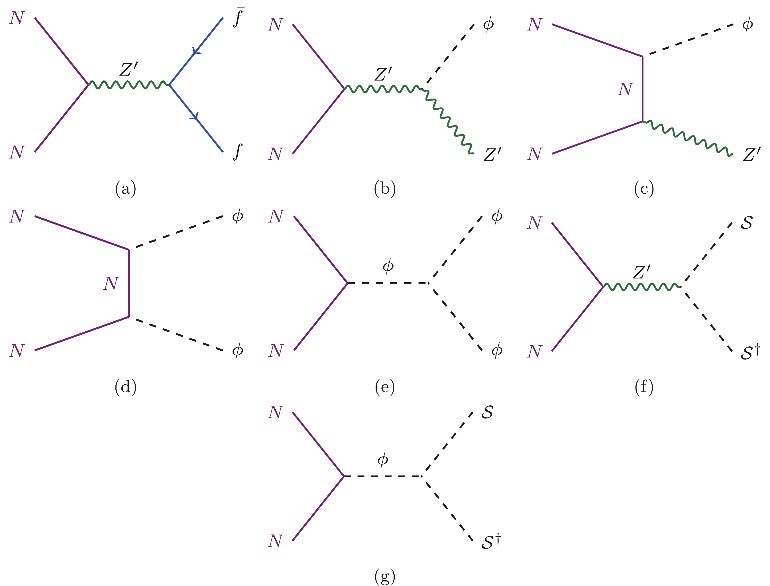

Figure 2.  (color online) Feynman diagram for the process (a) $N N \to f\bar{f}$, (b) and (c) $NN \to Z^\prime \Phi$, (d) and (e) $NN \to \Phi\Phi$, and (f) and (g) $NN \to {\cal{S}} {\cal{S}}^\dagger$.

The Boltzmann equations, which govern the evolution of the RHN number density and the lepton asymmetry, are given by

where $z\equiv m_N/T$ is a dimensionless parameter, $H_N\equiv$$H(z = 1)\simeq 17m_N^2/M_{\rm{Pl}}$ is the Hubble expansion rate at temperature $T = m_N$, $n_\gamma = 2T^3\zeta(3)/\pi^2$ is the number density of photons, and $\eta_N\equiv n_N/n_\gamma$ is the normalized number density of RHNs (similarly $\eta_{\Delta L} = (n_L-n_{\bar{L}})/n_\gamma$ for the lepton asymmetry). $\gamma$ represents the various thermalized interaction rates: $\gamma_D$ is for the RHN decay $N_{1,\,2} \to \ell_L H$, and $\gamma_{s} = \gamma_{H s} + \gamma_{Vs}$ and $\gamma_{t} = \gamma_{H t} + \gamma_{V t}$ are the standard $\Delta L = 1$ scattering processes as in Refs. [35, 67], with the subscripts $s,t$ denoting respectively the s and t-channel exchange of the SM Higgs doublet H or the SM gauge bosons $V = W_{i},\,B$ (with $i = 1,2,3$) before EWSB. Here, the integration over different momenta has already been performed, assuming implicitly kinetic equilibrium. The new scattering processes in our model in Fig. 2 correspond to the scattering rates $\gamma_{NN}$ in Eq. (19), and all the corresponding reduced cross sections $\hat{\sigma} (NN \to$$f\bar{f},\, Z'\phi, \, \phi\phi, {\cal{S}} {\cal{S}}^\dagger)$ are provided in Appendix C. The prefactor of 2 in Eq. (19) accounts for the reduction of RHN by a unit of two. The thermal corrections to the SM particles are included in the calculations [67, 68]. If the $\gamma_{NN}$ term is comparable or larger than the other terms on the right side of Eq. (19), these extra processes in Fig. 2 could significantly dilute the RHN number density before the sphaleron decoupling temperature $T_c\simeq 131.7$ GeV [69], thus potentially making type-I seesaw freeze-out leptogenesis ineffective. Then, we can set limits on the heavy particle masses and the couplings in the conformal $U(1)_{B-L}$ model.

To be specific, we considered two distinct scenarios, as follows:

(i) without the hidden scalar ${\cal{S}}$ involved in the lepton asymmetry generation in the RHN decay, and

(ii) with the scalar ${\cal{S}}$ involved in leptogenesis.

The case (i) corresponds to the limit of $m_{\cal{S}} \gg m_N$ and the case (ii) to the relation $m_{\cal{S}} \lesssim m_N$. In both cases, the dilution effect depends on the effective neutrino mass $\widetilde{m}\equiv v^2 (Y_D^{\dagger} Y_D)_{11}/m_N$ (or effectively on the Yukawa coupling $Y_D$) and the CP asymmetry ε. As in this study we were mostly concerned with the role of the new particles $Z'$, ϕ, and ${\cal{S}}$ in resonant leptogenesis, we did not consider the flavor structure details in the neutrino sector, but fixed $\widetilde{m}\simeq \sqrt{\Delta m^2_{\rm{atm}}} \simeq 50 \, {\rm{meV}}$, without any significant tuning or cancellation in the type-I seesaw formula for light neutrino masses [41]. A large ε can then be generated by the resonant enhancement mechanism, increasing to order one if $\Delta m_N \sim \Gamma_N$, where $\Gamma_N$ is the averaged RHN decay width [36, 64]. For concreteness, we adopt the value of $\varepsilon_{} = 10^{-2}$ throughout this paper.

In the strong washout regime, the RHN is typically close to the thermal equilibrium, i.e., $|\eta_N / \eta_N^{\rm{eq}} - 1| \ll 1$. In this case, the r.h.s. of Eq. (19) can be simplified as

and the leptogenesis constraints on the conformal model in this paper can thus be qualitatively obtained by requiring that $4 \gamma_{NN} \lesssim \gamma_D + \gamma_{s} + 2\gamma_{t}$. In most of the parameter space of interest, it is a good approximation to solve Eqs. (19) and (20) by taking the equilibrium limit $\eta_N \simeq \eta_N^{\rm{eq}}$. In this case, the final lepton asymmetry around the sphaleron decoupling temperature $T_c \simeq 131.7$ GeV can be factorized as [70]

with the effective K-factor

Without the dilution term $\gamma_{NN}$, we will recover the standard resonant leptogenesis. In this case, the lepton asymmetry $\eta_{\Delta L}$ will depend on the rates $\gamma_{D,\, s,\, t}$ for RHN decay and scattering processes; RHN width $\Gamma_N$ and the CP asymmetry ε, which are functions of the RHN mass $m_N$; the coupling matrix $Y_D$; and the mass splitting $\Delta m_N$. With the extra dilution processes in Eq. (18), the final lepton asymmetry will also depend on the masses of $Z'$, ϕ, and their couplings to the SM matter and RHNs. In the presence of ${\cal{S}}$, the mass $m_{\cal{S}}$ and its couplings to $Z'$ and ϕ will also affect the lepton asymmetry. In short, as long as the $\gamma_{NN}$ term is large compared to the other terms in Eq. (22), the lepton asymmetry will be suppressed. Throughout this paper, we follow this analytical approximation to derive the constraints and switch to the numerical solutions whenever necessary.

In case (i) without the hidden scalar ${\cal{S}}$, the dilution effect depends on $m_N$, the $Z'$ mass $m_{Z'}$, the conformal scalar mass $m_\phi$, and the quartic coupling $\lambda_\phi$; the last three are functions of the gauge coupling $g_{BL}$ and the $B-L$ scale $v_{BL}$ in the conformal theory, as shown in Eqs. (5), (7), and (26), respectively. Therefore, we chose the free parameters to be $m_N$, $g_{BL}$, and $v_{BL}$ in the conformal model, with the Yukawa coupling $Y_\phi$ determined by the RHN mass for fixed $v_{BL}$, which enters some of the diagrams in Fig. 2. For the three benchmark values of $g_{BL} = 0.1,\, 0.3,\,1$ in Table 2, the LHC dilepton limits on $v_{BL}$ are shown as the horizontal dashed red, green, and blue lines, respectively, in the left panel of Fig. 3. As stated in Ref. [41], in the case without ${\cal{S}}$, if the RHN mass $m_N \lesssim m_\phi$ and $2m_N \lesssim m_\phi + m_{Z'}$, the dilution is dominated by the $Z'$ mediated process $NN \to f \bar{f}$, benefiting from the (almost) massless fermions in the final state and the large number of degrees of freedom. The clear resonance structure can be seen in the left panel of Fig. 3, corresponding to the inverse decay process $N N \to Z'$ with the subsequent decay of the on-shell $Z'$ boson into SM fermions, which largely enhances the dilution effect. For sufficiently heavy RHNs with $m_N \gtrsim m_\phi$ and/or $2m_N \gtrsim m_\phi + m_{Z'}$, the processes $NN \to \phi\phi$ and/or $NN \to Z'\phi$ are also important, which are suppressed by the small Yukawa coupling $Y_\phi$ when $m_N \ll v_{BL}$. The effects of the different processes in Eq. (18) on the dilution of lepton asymmetry are additive; therefore, the dilution effect does not depend on the branching factions of the RHN annihilation processes. In the left panel of Fig. 3, all the red, green, and blue shaded regions are falsified by the extra diluting processes.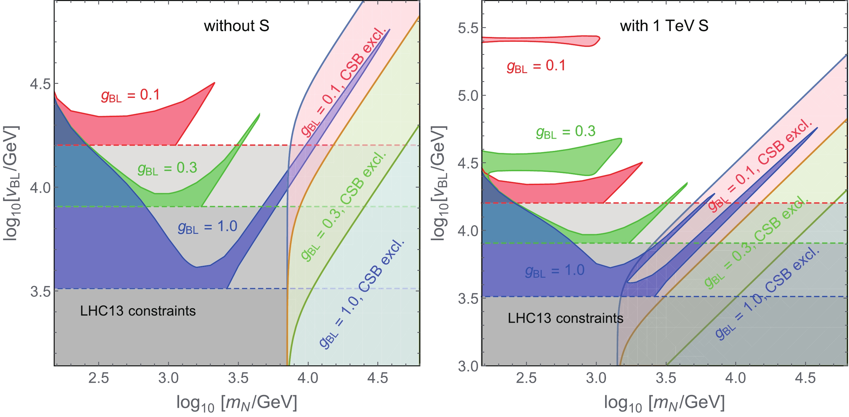

Figure 3.  (color online) Parameter space for leptogenesis for case (i) without ${\cal{S}}$ (left) and case (ii) with a 1 TeV ${\cal{S}}$. The gray regions are excluded by the dilepton limits on the $Z'$ mass (cf. Fig. 1 and Table 2), and the red, green and blue shaded regions are falsified by the processes shown in Fig. 2, with $g_{BL} = 0.1$, $0.3$, and $1$, respectively. The lighter shaded regions are excluded by the condition $m_\phi^2>0$ in Eq. (7).

When the hidden scalar mass $m_{S} \lesssim m_N$, the process $NN \to {\cal{S}} {\cal{S}}^\dagger$ would contribute to the dilution of lepton asymmetry generation, which corresponds to case (ii). This process is mediated by the $Z'$ and ϕ bosons, with the Feynman diagrams shown in Figs. 2(f) and (g). With the dashed curves in Fig. 1, the dilepton limits on the $Z'$ mass and the $v_{BL}$ scale are slightly lower than the case without ${\cal{S}}$, as shown in Table 2. The $Z'$ mediated process $NN \to Z' \to {\cal{S}} {\cal{S}}^\dagger$, however, can not complete the processes $NN \to ff$ as a result of the large degrees of freedom in the SM, unless the $B-L$ charge $n_{\cal{S}}$ of ${\cal{S}}$ is very large. Meanwhile, the cross section $\sigma (NN \to$$\phi \to {\cal{S}} {\cal{S}}^\dagger)$ in the scalar portal is proportional to the trilinear scalar coupling $(\lambda_{\phi S} v_{BL})^2$, which might significantly enhance the cross section when the $v_{BL}$ scale is large. Compared to the case without ${\cal{S}}$, the new scalar portal opens the possibility of new resonance, due to the relation $2E_N \simeq m_\phi$ (with $E_N$ the RHN energy) before the RHN decays. This corresponds to the extra peak structures in the right panel of Fig. 3, where for the sake of concreteness, we have fixed the hidden scalar mass as $m_{S} =$$1$ TeV. As in the left panel of Fig. 3, all the red, green, and blue shaded regions are falsified by the diluting processes, which reduce the RHN number by two units.

In short, all the red, green, and blue shaded regions in both panels of Fig. 3 are falsified by the Feynman diagrams in Fig. 2; for a viable leptogenesis framework to generate the baryon asymmetry in the early Universe, parameters in the unshaded regions in Fig. 3 should be chosen. Approximately, when the gauge coupling $g_{BL}$ (and the quartic coupling $\lambda_{\phi S}$) increases, the (reduced) cross sections for the dilution processes become larger, and the allowed parameter space shrinks significantly, depending on the RHN mass $m_N$. The bounds from the correct symmetry breaking (CSB) condition imposed by $m_\phi^2>0$ (see Eq. (7)) are also presented in the two panels of Fig. 3, which exclude sizable regions in the parameter space of $m_N$ and $v_{BL}$, as indicated by the light shaded regions. Furthermore, as seen in Fig. 3, the CSB constraints are largely complementary to the limits from leptogenesis.

As seen in Fig. 2, the quartic coupling $\lambda_\phi$ induces the channel $N N \to \phi^\ast \to \phi\phi$. However, this channel subleads to the channels $N N \to f \bar{f}$, with the latter enhanced by the large degrees of freedom in the SM. Therefore, the quartic coupling $\lambda_\phi$ is not very important for the dilution effect in resonant leptogenesis. One should also note that $\lambda_\phi$ is loop-induced and suppressed by the factor of $1/16\pi^2$ (see Eqs. (7) and (26)).

As the Universe cools, the EWSB is induced by the dynamical breaking of the $U(1)_{B-L}$, i.e., phase transition. If the phase transition is of strong first-order, GWs can be produced and probed by the space-based interferometers like LISA. In this section, we first demonstrate the calculative approach of the phase transition analogous to that in Ref. [31]. The phase transition dynamics is determined by the thermal potential as follows:

where

which is obtained from Eq. (4) after considering the matching condition at $\mu = v_{BL}$

The finite temperature corrections to the effective potential at one-loop are given by [71]

where the functions

with the + ($-$) sign corresponding to bosonic (fermionic) contributions. Here, to appropriately describe the behaviors at high and low temperatures, the integrals $J_{B, F}$ can be expressed as a sum of the second kind of modified Bessel functions $K_2(x)$ [72]:

As in Ref. [31], the dominant contributions come from the hidden scalar ${\cal{S}}$, RHNs $N_i$, and the extra gauge field $Z'$. The field-dependent mass and thermal corrections are given respectively as

Our study indicates that increasing the RHN masses may lead to a decrease in the phase transition temperature, while the RHN mass is severely bounded by the EWSB conditions given in Eq. (7). The hidden scalar ${\cal{S}}$ is useful for generating the proper vacuum barrier at the phase transition temperature. We note that the phase transition can be sensitive to the mass of ${\cal{S}}$ and the coupling $\lambda_{\phi S}$ for fixed $m_{Z'}$ and $m_N$.

The bounce configuration of the nucleated bubble, i.e., the bounce configuration of the field that connects the $U(1)_{B-L}$ broken vacuum (true vacuum) and the $U(1)_{B-L}$ conserving vacuum (false vacuum), can be obtained by extremizing

through solving the equation of motion for $\phi_b$ (which is the ϕ field for the scenario under study),

with the following boundary conditions:

At the nucleation temperature $T_n$, the thermal tunneling probability for bubble nucleation per horizon volume and per horizon time is of order unity with [73-75]

Two parameters are crucial for the calculations of GW radiation:

● $\alpha$, which describes the strength of the phase transition and is defined as the energy density released from the phase transition $\Delta \rho$ normalized by the radiation energy density:

where $\rho_R = \pi^2 g_\star T_*^4/30$ is the total radiation energy density with $g_\ast$ and $T_\ast$ respectively the relativistic degrees of freedom and temperature at the time of phase transition.

● β, which approximately describes the inverse time duration of the strong first order phase transition and is related to the peak frequency of the GW spectrum. It can be calculated from the action $S_3$ in Eq. (35) through

where $H_n$ is the Hubble parameter at the bubble nucleation temperature $T_n$.

In Ref. [76], the authors considered the “neutrino option” model, where the contributions of the real singlet and the RHNs dominate the phase transition and a significant supercooling is predicted [15-17, 21, 77, 78]. In our model considered here, there is no significant supercooling and the phase transition occurs with a relatively small $\alpha \sim O(10^{-1})$. We therefore have $T_*\approx T_n$ for the calculation of the GW spectrum. We are now ready to calculate the stochastic GW background generated at the first-order phase transition. Significant progress has been made in recent years on the calculations of GWs from phase transitions (e.g., see Refs. [79-81] for recent reviews). For the scenario studied here, it is now generally believed that the dominant source for the GW production in this process is the sound waves (SWs) in the plasma, which lasts long after the phase transition is completed [82, 83], though the bubble collision contribution has also been theoretically well modeled [84-91]. Another contribution comes from the magnetohydrodynamic (MHD) turbulence in the magnetized plasma with high Reynolds number [92, 93]. The total resultant energy density spectrum can be approximated by the following linear summation of the individual contributions mentioned above:

The dominant GW spectrum from SWs can be found by fitting to the result of numerical simulations based on the fluid-order parameter field model [15, 16, 77, 83]:

where $v_w$ is the bubble wall velocity; $\tau_{\rm{SW}}$ is the lifetime of SWs; $\kappa_v$ is the fraction of the released energy that is transferred to the kinetic energy of the plasma and can be calculated by analyzing the hydrodynamics around a single bubble for a given set of $(v_w, \alpha)$ [94]; and $f_{\rm{SW}}$ is the present peak frequency of the spectrum, given by

This spectrum, when the factor Υ is neglected, is obtained by assuming a very long lifetime, i.e., $\tau_{\rm{SW}} \rightarrow \infty$ [83]. However, the SWs can be disrupted by the onset of shocks and turbulence, and damped by other dissipative processes [83]. Therefore, its lifetime is usually smaller than a Hubble time [15, 16, 77]. In a recent thorough analysis of GW production in the expanding universe [95], it was found that the additional factor Υ needs to be included, which suppresses the spectrum. For a phase transition happening in a radiation dominated universe, it is given by [95]

Its value depends on the lifetime $\tau_{\rm{SW}}$, which can be chosen as the timescale for the onset of the turbulence [81] as

Here, $R_{\ast}$ is the mean bubble separation and is related to β through the relation $R_{\ast}(t) = (8\pi)^{1/3} {v_w}/{\beta}$ for exponential nucleation (see [96] for a derivation in the Minkowski spacetime and see [95] for the derivation in a generic expanding universe). Moreover, $\bar{U}_f$ is the root-mean-square (RMS) fluid velocity and can be expressed in terms of $\alpha$ and $\kappa_v$ [15, 97, 98]

The wall velocity $v_w$ should be calculated from the microdynamics, but it is usually taken as a free parameter due to the theoretical uncertainty of its determination [99-102]. We follow the same strategy and choose the value of $v_w$, which corresponds to the Jouguet detonation, given by [103]

The GW spectrum from the MHD turbulence can be theoretically modelled with inputs of the magnetic and turbulence power spectra [92, 104-106], and improved by numerically evolving the MHD equations [107, 108]. A fitting formula is also available, given by [92, 93]:

where the inverse Hubble time $h_\ast$ at the time of EWPT is

and the peak frequency $f_{\rm{MHD}}$ is given by

The energy fraction $\kappa_{\rm{MHD}}$ transferred to the MHD turbulence is uncertain as of now and can vary between 5% and 10% of $\kappa_v$ [83]. Here, we tentatively take $\kappa_{\rm{MHD}} = 0.1 \kappa_v$.

To assess the discovery prospects of the GW spectra, we calculated the signal-to-noise ratio (SNR) [79] as follows:

where $h^2 \Omega_{\rm{exp}}(f)$ is the experimental sensitivity for the detectors and ${\cal{T}}$ is the mission duration (in unit of year) for each experiment.

The expected GW energy spectra for the three different $g_{BL}$ values (see Table 2) are shown in Fig. 4. The color-shaded regions on the top are the sensitive regions for several proposed space-based GW experiments. Six benchmark scenarios with $g_{BL} = 0.1$, 0.3, 1 and two different values of $m_{\cal{S}}$ are shown respectively as the long and short dashed lines in the left, middle, and right panels of Fig. 4. The values of $m_{Z'}$, $m_N$, and $m_{\cal{S}}$ were chosen to satisfy the current LHC constraints on the $Z'$ mass in Table 2 and the leptogenesis limits in Fig. 3. The three panels of Fig. 4 demonstrate that the amplitudes of GW signal spectra decrease as $g_{BL}$ increases, implying that the GW prospects are weaker when the $B-L$ charge of the hidden scalar ${\cal{S}}$ is large. Furthermore, a larger hidden scalar mass leads to a lower GW amplitude and a higher peak frequency for the GW spectrum, which corresponds to a larger $m_\phi$ and a larger $\lambda_\phi$, as can be seen from Eqs. (7) and (26). Moreover, as seen in Fig. 4, the GW spectra of the following three benchmark scenarios,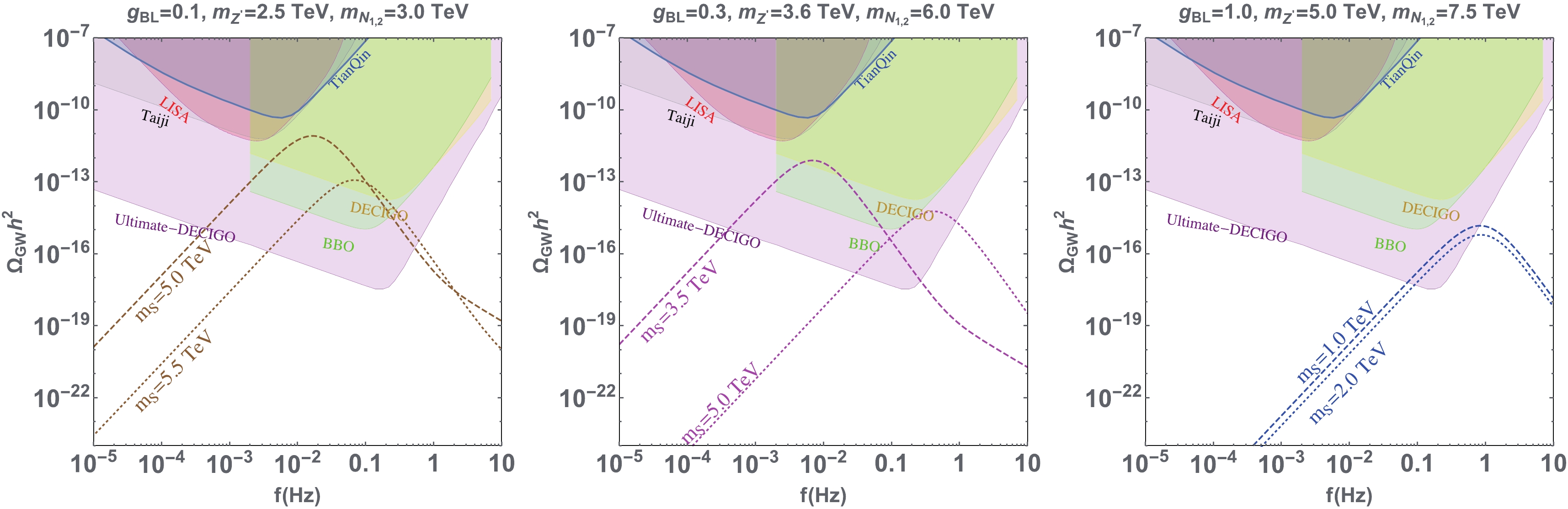

Figure 4.  (color online) The expected GW spectra for six benchmark scenarios in the conformal $U(1)_{B-L}$ model, shown as the long and short dashed curves, with $g_{BL} = 0.1$ (left), 0.3 (middle), and 1 (right) and two different values of $m_{\cal{S}}$. The shaded regions denote the GW prospects at LISA [24], Taiji [26], TianQin [27], BBO [28], DECIGO [29], and Ultimate-DECIGO [30].

can be probed in the far-future GW experiment, Ultimate-DECIGO.

In this paper, a hidden complex singlet scalar ${\cal{S}}$ is introduced to the $U(1)_{B-L}$ extension of the SM with classical conformal symmetry, which affects the dynamical EWSB by dimensional transmutation through the Coleman-Weinberg mechanism. As seen in Fig. 3, the correct spontaneous breaking of the U(1)$_{B-L}$ symmetry restricts the scales of the hidden scalar, and in a sizable region of the parameter space, the resonant leptogenesis mechanism is disturbed by the hidden scalar ${\cal{S}}$, depending on the mass hierarchy between it and the RHNs. As exemplified in Fig. 4, for smaller gauge coupling $g_{BL}$, a relatively light ${\cal{S}}$ at the TeV-scale is crucial to realize a strongly first-order phase transition, and produce GW signals to be probed by future GW experiments. It was found that the GW search is very useful to probe the hidden scalar ${\cal{S}}$ in the conformal $U(1)_{B-L}$ theory, which is difficult to directly search for at the high-energy colliders.

We would like to thank the Center for High Energy Physics, Peking University; the Institute of Theoretical Physics, Chinese Academy of Sciences; the Tsung-Dao Lee Institute; and the Institute of High Energy Physics, Chinese Academy of Sciences for generous hospitality, where the study was partially conducted.

Following Ref. [109], the RGEs for the scalar quartic couplings in the conformal $U(1)_{B-L}$ model read

with

where $g_1^2 = 5 g_Y^2/3$; $g_{2,\,Y}$ is the gauge coupling for the SM gauge groups $U(1)_Y$ and $SU(2)_L$; and $y_t$ is the SM top Yukawa coupling. For simplicity we neglected all other Yukawa couplings in the SM as well as the coupling matrix $Y_D$, which are much smaller. For the top quark Yukawa coupling $y_t$ and the coupling matrix $Y_\phi$ for the three RHNs, the RGEs are respectively

and the RGEs for the gauge couplings are given by

where $g_3$ is the gauge coupling for the SM gauge group $SU(3)_C$.

For the sake of completeness, we also checked the limits on the conformal $U(1)_{B-L}$ model from vacuum stability and perturbativity. The one-loop RGEs for all the quartic, Yukawa, and gauge couplings are presented in Appendix A, and the tree-level stability conditions are given below, which are consistent with those given in Ref. [110] (The two-loop level vacuum stability conditions in a different conformal $B-L$ theory has been studied in Ref. [111]):

With the RGEs in Appendix A and the initial conditions for all SM couplings at the scale $\mu = m_t$ (where $m_t$ is the top quark mass), we ran all the couplings up to the Planck scale $\mu = M_{\rm{Pl}} = 1.22 \times 10^{19}$ GeV. Then, using the relations in Eq. (B1), we could determine the Landau pole and vacuum stability bounds on the quartic couplings, the $U(1)_{B-L}$ gauge couplings $g_{BL}$, and the $B-L$ charge $n_{\cal{S}}$ of the hidden scalar ${\cal{S}}$.

As a result, the vacuum stability issue is not better in the SM as the GW prospects of the conformal $U(1)_{B-L}$ model prefer small quartic couplings of $\lambda_{HS,\,P}$. Furthermore, a large Yukawa coupling $Y_\phi$ for the RHNs would result in the Landau pole problem, as they tend to dominate the running of the quartic couplings at sufficiently high scale. The Landau pole appears at a scale much lower than $M_{\rm{Pl}}$ for the benchmark scenarios in the middle and right panels of Fig. 4; as a comparison, the scenarios in the left panel of Fig. 4 are much better, benefitting from a smaller coupling of $g_{BL} = 0.1$. The vacuum stability and Landau pole limits on the RHN mass $m_N$ and $m_{\cal{S}}$ with the hidden scalar charge $n_{\cal{S}} = 1$ are shown in Fig. B1 by the gray and orange shaded regions, respectively. As a good approximation, the limits in Fig. B1 are not sensitive to other couplings in the conformal $U(1)_{B-L}$ model.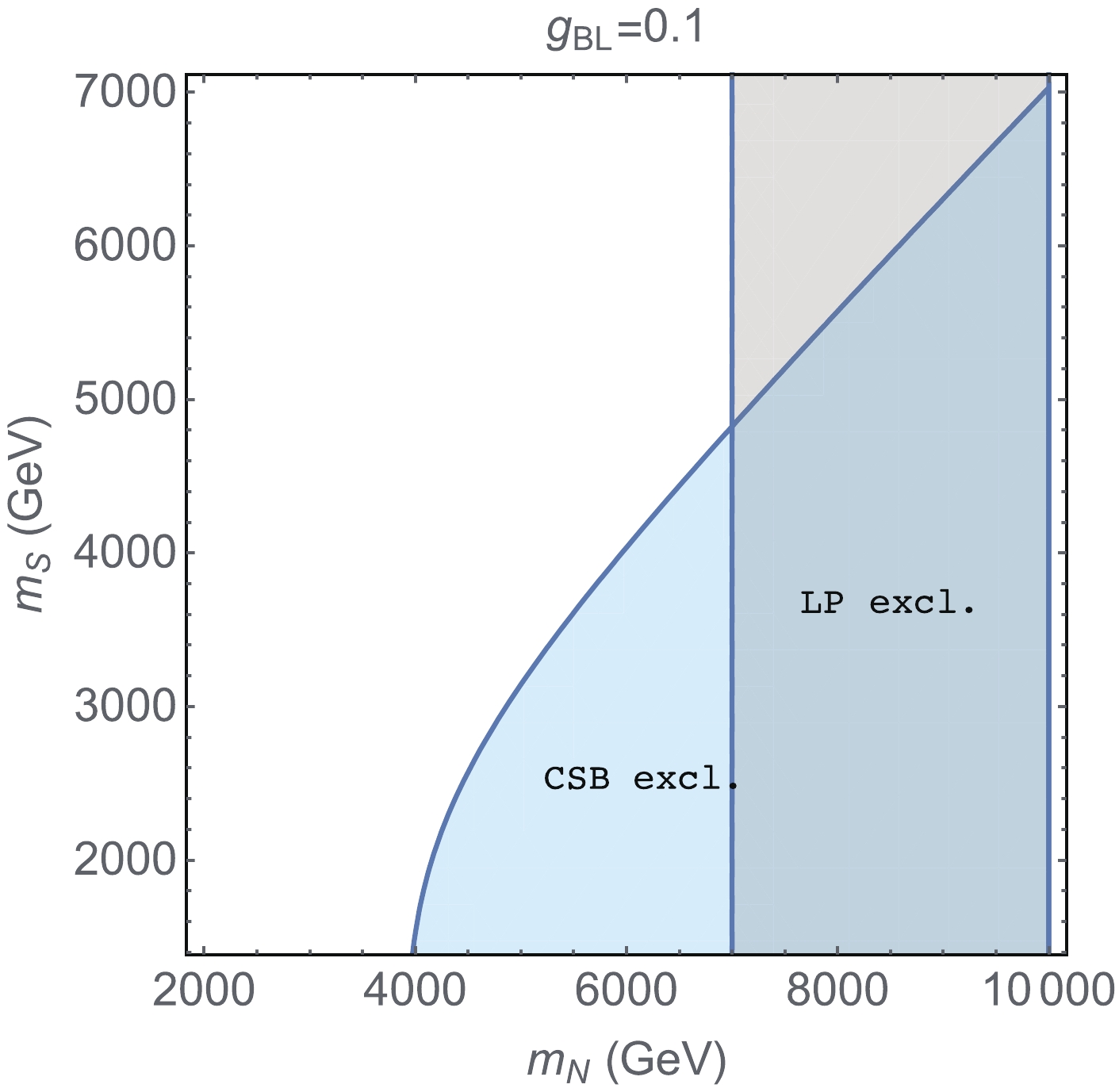

Figure B1.  (color online) Landau pole (orange) and vacuum stability (gray) excluded regions for the $g_{BL}=0.1$ scenarios given in the left panel of Fig. 4.

In this appendix, we list the explicit analytical formulas for the reduced cross sections for various $2\leftrightarrow 2$ scatterings involving the RHNs used in our leptogenesis calculations in Section III. All the relevant Feynman diagrams can be found in Fig. 2. The calculations follow closely Ref. [41]. For the fermionic channels,

with $x = s/m_N^2$, $w = m_{Z'}^2 / m_N^2$, and the symmetry factor $S_f = 1$ for the charged fermions and $1/4$ for neutrinos. For the bosonic channels,

with the ${\cal{A}}_{SS}$ and ${\cal{A}}_{VS}$ terms given as

where $r = m_{\phi}^2 / m_N^2$ and

At the $Z'$ resonance, i.e., $m_{Z'} \simeq 2 m_N$, the propagator $1/|x-w|$ should be modified accordingly to include the $Z'$ width. For the hidden scalar channel,

with $y = m_{S}^2 / m_N^2$, and