


 Abstract
 HTML
HTML Reference
 Related
 PDF
PDF


-
The allowed regions for the neutrino oscillation parameters, including neutrino mass squared differences, leptonic mixing angles, and the Dirac CP violating phase, taken from Ref. [1], are shown in Table 1. This confirms that the Standard Model (SM) must be extended to explain these experimental data.
Parameters $\mathrm{Normal \; Hierarchy\, (NH)}$ 

$\mathrm{Inverted \; hierarchy\, (IH)}$ 

$ \mathrm{bfp}\pm 1\sigma $ 

$ \mathrm{bfp}\pm 1\sigma $ 

$ \sin^2\theta_{12} $ 

$ 0.318\pm 0.016 $ 

$ 0.318\pm 0.016 $ 

$ \sin^2\theta_{23} $ 

$ 0.574\pm 0.014 $ 

$ 0.578^{+0.010}_{-0.017} $ 

$ \dfrac{\sin^2\theta_{13}}{10^{-2}} $ 

$ 2.200^{+0.069}_{-0.062} $ 

$ 2.225^{+0.064}_{-0.070} $ 

$\delta_{\rm CP}/\pi$ 

$ 1.08^{+0.13}_{-0.12} $ 

$ 1.58^{+0.15}_{-0.16} $ 

$ \dfrac{\Delta m^2_{21}}{10^{-5} \, \mathrm{eV}^2} $ 

$ 7.50^{+0.22}_{-0.20} $ 

$ 7.50^{+0.22}_{-0.20} $ 

$ \dfrac{|\Delta m^2_{31}|}{10^{-3} \, \mathrm{eV}^2} $ 

$ 2.55^{+0.02}_{-0.03} $ 

$ 2.45^{+0.02}_{-0.03} $ 

Table 1. Neutrino oscillation parameters taken from Ref. [1].
Among various extensions of the SM, the
$ B-L $ gauge model [2-21] is a promising candidate because it can explain various phenomena, such as the neutrino mass [14], leptogenesis [7, 21], dark matter [9-13, 16], the muon anomalous magnetic moment [14], gravitational wave radiation [8], and inflation [20]. However, by itself, this model cannot give a natural explanation for fermion mixing. Non-Abelian discrete symmetries have shown many outstanding advantages in explaining the observed patterns of fermion masses and mixing, and have been widely used in literature.An observed lepton mixing scenario can be successfully described using the cobimaximal mixing pattern (a pattern that predicts
$ \theta_{13} \neq 0,\, \theta_{23} = \dfrac{\pi}{4} $ and$ \delta_{\rm CP} = -\dfrac{\pi}{2} $ ), which has recently gained wider attention [22-29]. In order to explain the cobimaximal neutrino mixing pattern, alternative discrete symmetries have been used [22-29] with more than one$SU(2)_{L}$ Higgs doublet. However, the cobimaximal neutrino mixing pattern has not previously been considered in models with$ Q_4 $ symmetry. There are substantial differences between previous studies and this study regarding the explanation of the cobimaximal neutrino mixing pattern [22-29], namely, the cobimaximal lepton mixing form obtained with$ A_4 $ symmetry and three$ SU(2)_L $ Higgs doublets in the lepton sector with a general neutrino mass matrix [23], in one loop with the symmetry$ Z_2\times A_4\times Z_2\times U(1)_D $ and two$ SU(2)_L $ Higgs doublets [24], with the symmetry$ S_3\times Z_2 $ and two$ SU(2)_L $ doublets [25], with the symmetry$ S_3\times Z_2 $ and four$ SU(2)_L $ doublets [26], with the symmetry$ U(1)_\mathcal{X} \times U(1)_L \times U(1)_D \times \Delta(27)\times $ $ Z_2\times Z_3 $ and three$ SU(2)_L $ doublets [27], with the symmetry$ U(1)_\mathcal{X} \times \Delta(27)\times Z_4 \times R_L $ and four$ SU(2)_L $ doublets [28], and with the symmetry$ \Delta(27)\times Z_2 \times Z_{10} $ and two$ SU(2)_L $ doublets [29]. In this study, we suggest a non-renormalizable gauge$ B-L $ model based on the flavor symmetry$ Q_4\times Z_{4} \times Z_2 $ in which the first family of the left-handed lepton ($ \psi_{1L} $ ) is put in$ {1}_2 $ while the two others ($ \psi_{2, 3L} $ ) are put in$ {2} $ of$ Q_4 $ . For the right-handed leptons, the first family ($ l_{1R} $ ) is put in$ {1}_4 $ while the two others ($ l_{2,3R} $ ) are put in$ {2} $ of$ Q_4 $ . For the right-handed neutrinos, the first family ($ \nu_{1R} $ ) is put in$ {1}_1 $ while the two others ($ \nu_{2,3R} $ ) are put in$ {2} $ of$ Q_4 $ . As a result, the neutrino mass hierarchies, the tiny neutrino masses, and the cobimaximal lepton mixing pattern are generated at tree-level.$ Q_4 $ is the smallest group of the binary dihedral group$ Q_N $ with$ N = 4 $ , whose five irreducible representations are denoted as$ \mathbf{1}_k \, (k = 1,2,3,4) $ and$ \mathbf{2} $ , which are presented in Refs. [30-33]. We will consider the two-dimensional representation$ \mathbf{2} $ of$ Q_4 $ to be pseudo-real [30-33], i.e.,$ \mathbf{2}^*(a_1^*, a_2^*) = \mathbf{2}(a_2^*, -a_1^*) $ , and its basic tensor product rule is$ \begin{aligned}[b]\mathbf{2}(a_1, a_2) \otimes \mathbf{2}(b_1, b_2) = &\mathbf{1}_1(a_1b_2-a_2b_1) \oplus \mathbf{1}_2(a_1b_1-a_2b_2)\\& \oplus\mathbf{1}_3(a_1b_1+a_2b_2)\oplus \mathbf{1}_4(a_1b_2+a_2b_1).\end{aligned} $

This paper is organized as follows. In Section II, we present the particle content as well as the lepton sector of the model. Section III deals with the numerical analysis, and Section IV contains our conclusions.
-
In this study, the
$ B-L $ model [14, 17] is supplemented by$ Q_4\times Z_4 \times Z_2 $ symmetry; the total symmetry of our model is$ \Gamma \equiv SU(3)_C \times SU(2)_L\times U(1)_Y \times U(1)_{B-L} \times $ $ Q_4 \times Z_4 \times Z_2 $ . Moreover, three$ SU(2)_L $ singlet scalars ($ \chi, \rho, \eta $ ) with$ B-L = 0 $ and one$ SU(2)_L $ singlet scalar ($ \varphi $ ) with$ B-L = 2 $ are added to the$ B-L $ model particle content to describe the observed lepton mixing. The particle content of the model is summarized in Table 2.Fields $\psi_{1L}$ 

$\psi_{\alpha L}$ 

$l_{1R}$ 

$l_{\alpha R}$ 

$\nu_{1 R}$ 

$\nu_{\alpha R}$ 

H $\chi$ 

$\rho$ 

$\eta$ 

$\phi$ 

$\varphi$ 

${SU}(3)_{\rm C}$ 

${1}$ 

${1}$ 

${1}$ 

${1}$ 

${1}$ 

${1}$ 

${1}$ 

${1}$ 

${1}$ 

${1}$ 

${1}$ 

${1}$ 

${SU}(2)_L$ 

${2}$ 

${2}$ 

${1}$ 

${1}$ 

${1}$ 

${1}$ 

${2}$ 

${1}$ 

${1}$ 

${1}$ 

${1}$ 

${1}$ 

${U}(1)_Y$ 

$-\frac{1}{2}$ 

$-\frac{1}{2}$ 

$-1$ 

$-1$ 

$0$ 

$0$ 

$\frac{1}{2}$ 

$0$ 

$0$ 

$0$ 

$0$ 

$0$ 

$U(1)_{B-L}$ 

$-1$ 

$-1$ 

$-1$ 

$-1 $ 

$-1$ 

$-1$ 

$0$ 

$0$ 

$0$ 

$0$ 

$2$ 

$2$ 

$Q_4$ 

${1}_2$ 

${2}$ 

${1}_4$ 

${2}$ 

${1}_1$ 

${2}$ 

${1}_1$ 

${1}_3$ 

${1}_4$ 

${2}$ 

${1}_1$ 

${1}_2$ 

$Z_4$ 

$1$ 

$1$ 

$-i$ 

$-i$ 

i i i $1$ 

$1$ 

$1$ 

$-1$ 

$-1$ 

$Z_2$ 

$+$ 

$+$ 

$-$ 

$-$ 

$+$ 

$+$ 

$-$ 

$+$ 

$-$ 

$-$ 

$+$ 

$+$ 

Table 2. Particle and scalar content of the model (
$ \alpha = 2,3 $ ).The scalar potential minimum condition, as shown in Appendix A, yields the vacuum expectation value (VEV) of scalars.
$ \begin{aligned}[b] &\langle H \rangle = \left(0 \,\,v_H \right)^T,\quad \langle \chi \rangle = v_\chi, \quad\langle \rho \rangle = v_\rho, \\ & \langle \eta \rangle = (\langle \eta_1 \rangle, \; \langle \eta_{2} \rangle), \quad \langle \eta_1 \rangle = \langle \eta_2 \rangle = v_\eta, \\ &\langle \phi \rangle = v_\phi, \quad \langle \varphi \rangle = (\langle \varphi_1 \rangle,\; \langle \varphi_{2} \rangle), \quad \langle \varphi_1 \rangle = \langle \varphi_2 \rangle = v_\varphi. \end{aligned} $

(1) From the particle content given in Table 2 and the tensor products of
$ Q_4 $ , the charged lepton masses can arise from the couplings of$\bar{\psi}_{(1, \alpha) {L}} l_{(1, \alpha){R}}$ to scalars, where$\bar{\psi}_{1L} l_{1R}$ transform to$ \left(1, 2, -\dfrac{1}{2}, 0, {1}_3, -i, -\right) $ ,$\bar{\psi}_{1{L}} l_{ \alpha {R}}\sim \bar{\psi}_{ \alpha {L}} l_{1 {R}} $ $ \sim \left(1, 2, -\dfrac{1}{2}, 0, {2}, -i, -\right)$ , and$\bar{\psi}_{ \alpha {L}} l_{ \alpha {R}} \sim (1, 2, -\dfrac{1}{2}, $ $ 0, {1}_1 \oplus {1}_2$ $ \oplus \,{1}_3 $ $ \oplus{1}_4, -i, - ) $ . Thus, to generate masses for the charged leptons, we require one$ SU(2)_L $ doublet H and one$ SU(2)_L $ singlet$ \chi $ placed in$ \mathbf{1}_1 $ and$ \mathbf{1}_3 $ under$ Q_4 $ , respectively. The Yukawa interactions in the charged lepton sector are$\begin{aligned}[b] -\mathcal{L}^{\rm clep}_{Y} =& \frac{x^{cl}_{1}}{\Lambda} (\bar{\psi}_{1L} l_{1R})_{{1}_3} (H\chi)_{{1}_3} + x^{cl}_{2}\left(\bar{\psi}_{ \alpha L} l_{ \alpha R}\right)_{\mathbf{1}_1} H\\& + \frac{x^{cl}_{3}}{\Lambda} \left(\bar{\psi}_{ \alpha L} l_{ \alpha R}\right)_{\mathbf{1}_3} (H\chi)_{\mathbf{1}_3} + \mathrm{H.c.} \end{aligned} $

(2) It is noted that
$ (\overline{\psi}_{1 L} l_{1R}) H $ is forbidden by the$ Z_4 $ symmetry;$ (\overline{\psi}_{1 L} l_{1R})H\rho $ and$ (\overline{\psi}_{1 L} l_{1R})H\eta $ are forbidden by the$ Q_4 $ symmetry;$ (\overline{\psi}_{1 L} l_{1R})H\phi $ and$ (\overline{\psi}_{1 L} l_{1R})H\varphi $ are forbidden by two symmetries,$ Q_4 $ and$ B-L $ ;$ (\overline{\psi}_{1 L} l_{ \alpha R}) H $ and$ (\overline{\psi}_{1 L} l_{ \alpha R}) H\chi $ are forbidden by the$ Q_4 $ symmetry;$ (\overline{\psi}_{1 L} l_{ \alpha R})H\rho $ is forbidden by the$ Q_4 $ and$ Z_2 $ symmetries;$ (\overline{\psi}_{1 L} l_{ \alpha R})H\eta $ is forbidden by the$ Z_2 $ symmety;$ (\overline{\psi}_{1 L} l_{ \alpha R})H\phi $ and$ (\overline{\psi}_{1 L} l_{ \alpha R})H\varphi $ are forbidden by three symmetries,$ Q_4, Z_4 $ , and$ B-L $ ;$ (\overline{\psi}_{ \alpha L} l_{ \alpha R}) H\rho $ and$ (\overline{\psi}_{ \alpha L} l_{ \alpha R}) H\eta $ are forbidden by two symmetries,$ Q_4 $ and$ Z_2 $ ; and$ (\overline{\psi}_{ \alpha L} l_{ \alpha R})H\phi $ and$ (\overline{\psi}_{ \alpha L} l_{ \alpha R})H\varphi $ are forbidden by three symmetries,$ Q_4, Z_4 $ , and$ B-L $ . In the charged-lepton sector, the invariant Yukawa interactions are shown in Eq. (2). With the help of Eq. (1), the Lagrangian mass term of the charged leptons can be written in the form$ -\mathcal{L}^{\mathrm{mass}}_l = (\bar{l}_{1L},\bar{l}_{2L},\bar{l}_{3L}) {M}_l (l_{1R},l_{2R},l_{3R})^T+ {\rm H. c}, $

(3) where
$ {M}_l = \left( \begin{array}{ccc} a_l & \quad 0 & \quad 0 \\ 0 & \quad b_l& -c_l\\ 0 & \quad c_l & \quad b_l\\ \end{array} \right), $

(4) with
$a_l = \frac{x^{cl}_{1}}{\Lambda} v_H v_\chi, \quad b_l = x^{cl}_{2} v_H, \quad c_l = \frac{x^{cl}_{3}}{\Lambda} v_H v_\chi. $

(5) Let us first define a Hermitian matrix
$ m_l $ , given by$ {m}_l = {M}^+_L {M}_L = \left( \begin{array}{ccc} \alpha_{l} & 0 & 0 \\ 0 & \quad \beta_l& \quad {\rm i} \gamma_{l} \\ 0 & \quad -{\rm i} \gamma_{l} & \quad \beta_l \\ \end{array} \right), $

(6) where
$ \alpha_l = a_{0l}^2,\quad \beta_l = b_{0l}^2+c_{0l}^2,\quad \gamma_l = 2 b_{0l} c_{0l} \sin \varphi_{l}, $

(7) and
$ \varphi_l = \varphi_{b}-\varphi_{c}, \;\, a_{0l} = |a_l|, \;\, b_{0l} = |b_l|, \;\, c_{0l} = |c_l| $ , and$ \varphi_{b} = $ $ \arg (b_l),\; \varphi_{c} = \arg (c_l) $ .The matrix
${m}_l$ can be diagonalized by${u}_{{L, R}}$ , satisfying${u}^+_{{L}} {m}_l {u}_{{R}} = \mathrm{diag} (m^2_e, m^2_\mu, m^2_\tau)$ , where$ {u}_{L} = {u}_{R} = \frac{1}{\sqrt{2}}\left( \begin{array}{ccc} \sqrt{2} & 0 & 0 \\ 0 & \quad i & \quad i\\ 0 & \quad -1 & \quad 1 \\ \end{array} \right), $

(8) $ m^2_e = \alpha_{l}, \,\, m^2_{\mu, \tau} = \beta_{l}\mp \gamma_l. $

(9) Comparing the obtained result in Eq. (9) with the experimental values of the charged lepton masses at the weak scale taken from Ref. [34],
$ m_e = 0.51099 \;\mathrm{MeV}, m_\mu = $ $ 105.65837\;\mathrm{MeV},\; m_\tau = 1776.86 \;\mathrm{MeV} $ , we get$ \alpha_l = 0.261\; \mathrm{MeV},\; \beta_l = 1.58 \times 10^{6}\; \mathrm{MeV},\; \gamma_l = 1.57 \times 10^{6} \; \mathrm{MeV}. $

(10) Regarding the neutrino sector, the Dirac mass terms are generated from the couplings of
$ \bar{\psi}_{i L} \nu_{j R}\, (i,j = 1,2,3) $ to scalars, where$ \bar{\psi}_{1 L} \nu_{1 R}\sim (1, 2, \dfrac{1}{2}, 0, {1}_2, i, +) $ ,$ \bar{\psi}_{1 L} \nu_{ \alpha R}\sim \bar{\psi}_{ \alpha L} \nu_{1 R} $ $ \sim (1, 2, \dfrac{1}{2}, 0, {2}, i, +) $ , and$ \bar{\psi}_{ \alpha L} \nu_{ \alpha R}\sim (1, 2, \dfrac{1}{2}, 0, {1}_1\oplus $ $ {1}_2 \oplus{1}_3 \oplus{1}_4, $ $ i, +) $ . The Majorana neutrino masses are generated from the couplings of$ \bar{\nu}^c_{i R}\nu_{j R} \, (i,j = 1,2,3) $ to scalars, where$ \bar{\nu}^c_{1 R}\nu_{1 R}\sim (1, 1, 0, -2, {1}_1, -1, +) $ ,$\bar{\nu}^c_{1 R}\nu_{ \alpha R}\sim\bar{\nu}^c_{ \alpha R}\nu_{1 R}\sim (1, 1, 0, -2, $ $ {2}, -1, +)$ , and$ \bar{\nu}^c_{ \alpha R}\nu_{ \alpha R}\sim (1, 1, 0, -2, {1}_1\oplus{1}_2\oplus{1}_3\oplus $ $ {1}_4, -1, +) $ . The Yukawa interactions in the neutrino sector are$ \begin{align} -\mathcal{L}^{\nu}_{Y}= &\frac{x_{1\nu}}{\Lambda}(\bar{\psi}_{1 L} \nu_{ \alpha R}+\bar{\psi}_{ \alpha L} \nu_{1 R})_{2} (\widetilde{H}\eta)_{2}+\frac{x_{2\nu}}{\Lambda} \left(\bar{\psi}_{ \alpha L} \nu_{ \alpha R}\right)_{\mathbf{1}_3}(\widetilde{H}\rho)_{\mathbf{1}_3} \\ &+\frac{y_{1\nu}}{2} \left(\bar{\nu}^c_{1 R} \nu_{1 R}\right)\phi+\frac{y_{2\nu}}{2} \left(\bar{\nu}^c_{ \alpha R}\nu_{ \alpha R}\right)_{\mathbf{1}_2}\varphi +\mathrm{H.c.} \\[-5pt]\end{align} $

(11) In the neutrino sector,
$ (\overline{\psi}_{1 L} \nu_{1R}) \widetilde{H} $ and$ (\overline{\psi}_{1 L} \nu_{1R}) \widetilde{H}\chi $ are forbidden by two symmetries,$ Q_4 $ and$ Z_2 $ ;$ (\overline{\psi}_{1 L} \nu_{1R})\widetilde{H}\rho $ and$ (\overline{\psi}_{1 L} \nu_{1R})\widetilde{H}\eta $ are forbidden by the$ Q_4 $ symmetry;$ (\overline{\psi}_{1 L} \nu_{1R})\widetilde{H}\phi $ is forbidden by four symmetries,$ Q_4, Z_4, Z_2, B-L $ ;$ (\overline{\psi}_{1 L} \nu_{1R})\widetilde{H}\varphi $ is forbidden by three symmetries$ Z_4, Z_2 $ , and$ B-L $ .$ (\overline{\psi}_{1 L} \nu_{ \alpha R}) \widetilde{H} $ and$ (\overline{\psi}_{1 L} \nu_{ \alpha R}) \widetilde{H}\chi $ are forbidden by two symmetries,$ Q_4 $ and$ Z_2 $ ;$ (\overline{\psi}_{1 L} \nu_{ \alpha R})\widetilde{H}\rho $ is forbidden by the$ Q_4 $ symmetry;$ (\overline{\psi}_{1 L} \nu_{ \alpha R})\widetilde{H}\phi $ and$ (\overline{\psi}_{1 L} \nu_{ \alpha R})\widetilde{H}\varphi $ are forbidden by four symmetries,$ Q_4, Z_4, Z_2 $ , and$ B-L $ .$ (\overline{\psi}_{ \alpha L} \nu_{ \alpha R}) \widetilde{H} $ and$ (\overline{\psi}_{ \alpha L} \nu_{ \alpha R}) \widetilde{H}\chi $ are forbidden by the$ Z_2 $ symmetry;$ (\overline{\psi}_{ \alpha L} \nu_{ \alpha R})\widetilde{H}\eta $ is forbidden by the$ Q_4 $ symmetry;$ (\overline{\psi}_{ \alpha L} \nu_{ \alpha R})\widetilde{H}\phi $ and$ (\overline{\psi}_{ \alpha L} \nu_{ \alpha R})\widetilde{H}\varphi $ are forbidden by three symmetries,$ Z_4, Z_2 $ , and$ B-L $ . Furthermore,$ (\overline{\nu}^c_{1 R} \nu_{1 R}) H $ is forbidden by four symmetries,$ Y, B-L, Z_4 $ , and$ Z_2 $ ;$ (\overline{\nu}^c_{1 R} \nu_{1 R}) \chi $ is forbidden by three symmetries,$ B-L, Q_4 $ , and$ Z_4 $ ;$ (\overline{\nu}^c_{1 R} \nu_{1 R}) \rho $ and$ (\overline{\nu}^c_{1 R} \nu_{1 R}) \eta $ are forbidden by four symmetries,$ B-L, Q_4, Z_4 $ , and$ Z_2 $ ; and$ (\overline{\nu}^c_{1 R} \nu_{1 R}) \varphi $ is forbidden by the$ Q_4 $ symmetry.$ (\overline{\nu}^c_{1 R} \nu_{ \alpha R}) H $ is forbidden by five symmetries,$ Y, B-L, Q_4, Z_4 $ , and$ Z_2 $ ;$ (\overline{\nu}^c_{1 R} \nu_{ \alpha R}) \chi $ is forbidden by three symmetries,$ B-L, Q_4 $ , and$ Z_4 $ ;$ (\overline{\nu}^c_{1 R} \nu_{ \alpha R}) \rho $ and$ (\overline{\nu}^c_{1 R} \nu_{ \alpha R}) \eta $ are forbidden by four symmetries,$ B-L, Q_4, Z_4 $ , and$ Z_2 $ ; and$ (\overline{\nu}^c_{1R} \nu_{ \alpha R}) \varphi $ and$ (\overline{\nu}^c_{1 R} \nu_{ \alpha R}) \phi $ are forbidden by the$ Q_4 $ symmetry.$ (\overline{\nu}^c_{ \alpha R} \nu_{ \alpha R}) H $ is forbidden by four symmetries,$ Y, B-L, Z_4 $ , and$ Z_2 $ ;$ (\overline{\nu}^c_{ \alpha R} \nu_{ \alpha R}) \chi $ is forbidden by two symmetries,$ B-L $ and$ Z_4 $ ;$ (\overline{\nu}^c_{ \alpha R} \nu_{ \alpha R}) \rho $ is forbidden by three symmetries,$ B-L, Z_4 $ , and$ Z_2 $ ; and$ (\overline{\nu}^c_{ \alpha R} \nu_{ \alpha R}) \eta $ is forbidden by four symmetries,$ B-L, Q_4, Z_4 $ , and$ Z_2 $ . All other terms of the form$ (\overline{\nu}^c_{1 R} \nu_{1 R}) \Phi, \, (\overline{\nu}^c_{1 R} \nu_{ \alpha R})\Phi $ , and$ (\overline{\nu}^c_{ \alpha R} \nu_{ \alpha R})\Phi $ , where$ \Phi $ are the combinations of scalar fields such as$ H \chi, H\rho, H\eta, H\phi, H\varphi; \chi\rho, \chi\eta, \chi\phi, \chi\varphi $ , are forbidden by one or some of the model's symmetries. In addition,$ (\overline{\nu}^c_{ \alpha R} \nu_{ \alpha R})_{\mathbf{1}_1} \phi = (\overline{\nu}^c_{2 R} \nu_{3 R}-\overline{\nu}^c_{3 R} \nu_{2 R})_{\mathbf{1}_1} \phi = 0 $ . For the neutrino sector, the invariant Yukawa interactions are shown in Eq. (11).With the VEVs given in Eq. (1), we obtain the Dirac and Majorana neutrino mass matrices using the following:
$ M_D= \left( \begin{array}{ccc} 0 & \quad -a_D & \quad a_D \\ a_D & \quad 0 & \quad b_D \\ a_D & \quad b_D & 0 \\ \end{array} \right),\quad M_R = \left( \begin{array}{ccc} a_R & 0 & 0 \\ 0 & b_R & 0 \\ 0& 0 & -b_R \\ \end{array} \right), $

(12) where
$ \begin{aligned}[b] a_D=& \frac{x_{1\nu}}{\Lambda} v_H v_\eta,\\ b_D =& \frac{x_{2\nu}}{\Lambda} v_H v_\rho, \\a_R =& y_{1\nu} v_\phi,\\ b_R =& y_{2\nu} v_\varphi.\end{aligned}$

(13) The effective neutrino mass matrix is obtained through the type-I seesaw mechanism as follows:
$ {{M}}_{\mathrm{eff}}= -M_D {M}_R^{-1}M^T_D = \left( \begin{array}{ccc} 0 & \dfrac{a_D b_D}{b_R} & -\dfrac{a_D b_D}{b_R} \\ \dfrac{a_D b_D}{b_R} & \dfrac{b^2_D}{b_R}-\dfrac{a^2_D}{a_R} & \dfrac{a^2_D}{a_R} \\ -\dfrac{a_D b_D}{b_R} & \dfrac{a^2_D}{a_R} & -\dfrac{a^2_D}{a_R}-\dfrac{b^2_D}{b_R} \end{array} \right). $

(14) The mass matrix
$ {M}_{\mathrm{eff}} $ in Eq. (14) has three eigenvalues:$ m_1= 0, m_{2,3} = - \alpha \mp \beta, $

(15) with
$ \alpha= \frac{a_D^2}{a_R}, \,\,\, \beta = \frac{\sqrt{a_D^4 b_R^2+a_R^2 b_D^2 \left(2 a_D^2+ b_D^2\right)}}{a_R b_R}. $

(16) The corresponding mixing matrix is
$ \boldsymbol{K} = \left( \begin{array}{ccc} \dfrac{\kappa}{\sqrt{\kappa^2+2}} &\dfrac{\kappa_1}{\sqrt{\kappa^2_1+\tau^2_1+1}}&\dfrac{\kappa_2}{\sqrt{\kappa^2_2+\tau^2_2+1}}\\ -\dfrac{1}{\sqrt{\kappa^2+2}} &\dfrac{\tau_1}{\sqrt{\kappa^2_1+\tau^2_1+1}}&\dfrac{\tau_2}{\sqrt{\kappa^2_2+\tau^2_2+1}}\\ -\dfrac{1}{\sqrt{\kappa^2+2}} &\dfrac{1}{\sqrt{\kappa^2_1+\tau^2_1+1}} &\dfrac{1}{\sqrt{\kappa^2_2+\tau^2_2+1}} \end{array}\right), $

(17) where
$ \kappa, \kappa_{1,2} $ , and$ \tau_{1,2} $ are given by$ \begin{aligned}[b] &\kappa = \frac{ b_D}{a_D}, \quad\kappa_{1,2} = \frac{2 a_D a_R b_D}{a_R b_D^2+a_D^2 b_R \pm \sqrt{\Omega}}, \\&\tau_{1, 2} = \frac{\pm \sqrt{\Omega}-a_R \left(a_D^2+b_D^2\right)}{a_D^2 (a_R-b_R)}, \\ &\Omega = a_D^4 b_R^2+a_R^2 b_D^2 \left(2 a_D^2+b_D^2\right), \end{aligned} $

(18) which satisfy the following relations:
$\begin{aligned}[b]1 + \kappa_1 \kappa_2 + \tau_1 \tau_2& = 0, \\1 - \kappa \kappa_1 + \tau_1 =& 0, \\1 - \kappa \kappa_2 + \tau_2 =& 0. \end{aligned}$

(19) Whether the neutrino mass spectrum has a normal or inverted hierarchy depends on the sign of
$ \Delta m^2_{31} $ [34]. For NH,$ 0 = m_1\ll m_{2}\sim m_{3} $ . For IH,$ 0 = m_3\ll m_1\sim m_2 $ . The neutrino mass matrix$ M_{\mathrm{eff}} $ in Eq. (14) is diagonalized as$\begin{aligned}\\ {u}_{\nu }^T {M}_{\mathrm{eff}} {u}_{\nu } = \left\{ \begin{aligned} \left( \begin{array}{ccc} 0 & 0 & 0 \\ 0 & - \alpha - \beta & 0 \\ 0 & 0 & - \alpha + \beta \end{array} \right), \quad {u}_{\nu } = \left( \begin{array}{ccc} \dfrac{\kappa}{\sqrt{\kappa^2+2}} &\dfrac{\kappa_1}{\sqrt{\kappa^2_1+\tau^2_1+1}}&\dfrac{\kappa_2}{\sqrt{\kappa^2_2+\tau^2_2+1}}\\ -\dfrac{1}{\sqrt{\kappa^2+2}} &\dfrac{\tau_1}{\sqrt{\kappa^2_1+\tau^2_1+1}}&\dfrac{\tau_2}{\sqrt{\kappa^2_2+\tau^2_2+1}}\\ -\dfrac{1}{\sqrt{\kappa^2+2}} &\dfrac{1}{\sqrt{\kappa^2_1+\tau^2_1+1}} &\dfrac{1}{\sqrt{\kappa^2_2+\tau^2_2+1}} \end{array}\right) \quad {\rm{for}}\;{\rm{NH}}, \\[1em] \left( \begin{array}{ccc} - \alpha - \beta & 0 & 0 \\ 0 & - \alpha + \beta & 0 \\ 0 & 0 & 0 \end{array} \right) , \quad {u}_{\nu } = \left( \begin{array}{ccc} \dfrac{\kappa_1}{\sqrt{\kappa^2_1+\tau^2_1+1}}&\dfrac{\kappa_2}{\sqrt{\kappa^2_2+\tau^2_2+1}}& \dfrac{\kappa}{\sqrt{\kappa^2+2}}\\ \dfrac{\tau_1}{\sqrt{\kappa^2_1+\tau^2_1+1}}&\dfrac{\tau_2}{\sqrt{\kappa^2_2+\tau^2_2+1}}& -\dfrac{1}{\sqrt{\kappa^2+2}} \\ \dfrac{1}{\sqrt{\kappa^2_1+\tau^2_1+1}} &\dfrac{1}{\sqrt{\kappa^2_2+\tau^2_2+1}}& -\dfrac{1}{\sqrt{\kappa^2+2}} \end{array}\right) \quad {\rm{for}}\;{\rm{IH}}, \\\end{aligned} \right. \end{aligned} $ 
(20) where
$ \alpha, \;\beta $ ,$ \kappa, \;\kappa_{1,2} $ , and$ \tau_{1,2} $ are given in Eqs. (16) and (19). The corresponding leptonic mixing matrix is defined as follows:$ {U}_{\mathrm{Lep}} = {u}_{\mathrm{L}}^{\dagger} {u}_{\nu } = \left\{ \begin{aligned} \left( \begin{array}{ccc} \dfrac{\kappa}{\sqrt{\kappa^2+2}} & \dfrac{\kappa_1}{\sqrt{\kappa_1^2+\tau_1^2+1}} &\dfrac{\kappa_2}{\sqrt{\kappa_2^2+\tau_2^2+1}} \\ \dfrac{i+1}{\sqrt{2} \sqrt{\kappa^2+2}} & -\dfrac{1+i \tau_1}{\sqrt{2} \sqrt{\kappa_1^2+\tau_1^2+1}} & -\dfrac{1+i \tau_2}{\sqrt{2} \sqrt{\kappa_2^2+\tau_2^2+1}} \\ \dfrac{i-1}{\sqrt{2} \sqrt{\kappa^2+2}} & \quad \dfrac{1-i \tau_1}{\sqrt{2} \sqrt{\kappa_1^2+\tau_1^2+1}} & \quad \dfrac{1-i \tau_2}{\sqrt{2} \sqrt{\kappa_2^2+\tau_2^2+1}} \end{array} \right) \; \;{\rm{for}}\;{\rm{NH}}, \\ \left( \begin{array}{ccc} \dfrac{\kappa_1}{\sqrt{\kappa_1^2+\tau_1^2+1}} &\dfrac{\kappa_2}{\sqrt{\kappa_2^2+\tau_2^2+1}}& \dfrac{\kappa}{\sqrt{\kappa^2+2}} \\ -\dfrac{1+i \tau_1}{\sqrt{2} \sqrt{\kappa_1^2+\tau_1^2+1}} & -\dfrac{1+i \tau_2}{\sqrt{2} \sqrt{\kappa_2^2+\tau_2^2+1}}& \dfrac{i+1}{\sqrt{2} \sqrt{\kappa^2+2}} \\ \quad \dfrac{1-i \tau_1}{\sqrt{2} \sqrt{\kappa_1^2+\tau_1^2+1}} & \quad \dfrac{1-i \tau_2}{\sqrt{2} \sqrt{\kappa_2^2+\tau_2^2+1}}& \dfrac{i-1}{\sqrt{2} \sqrt{\kappa^2+2}} \\ \end{array} \right) \; \;{\rm{for}}\;{\rm{IH}}. \end{aligned} \right. $

(21) In the three neutrino oscillation picture [34-37], the leptonic Jarlskog invariant
$ J_{\rm CP} $ , which determines the magnitude of CP violation in neutrino oscillations and the lepton mixing angles, is obtained as follows:$ J_{\mathrm{CP}} = \mathrm{Im} \left({U}_{23} {U}^*_{13} {U}_{12} {U}^*_{22}\right) = s_{12}c_{12} s_{13} c_{13}^2s_{23}c_{23} \sin\delta,\quad\quad$

(22) $ s^2_{13} = |{U}_{13}|^2, \quad t^2_{12} = \left|\frac{{U}_{12}}{{U}_{11}}\right|^2,\quad t^2_{23} = \left|\frac{{U}_{2 3}}{{U}_{2 3}}\right|^2, $

(23) where
$ t_{ij} = \dfrac{s_{ij}}{c_{ij}},\, s_{ij} = \sin\theta_{ij},\, c_{ij} = \cos\theta_{ij}\, (ij = 12,23) $ with$ \theta_{12} $ ,$ \theta_{23} $ , and$ \theta_{13} $ are the solar angle, atmospheric angle, and reactor angle, respectively.Combining Eqs. (21), (22), and (23) yields
$ \frac{\kappa_2^2 \left(\tau_2^2-1\right)}{2 \left(\kappa_2^2+\tau_2^2+1\right) \left(2 \kappa_2^2+(\tau_2+1)^2\right)} = s_{12}c_{12} s_{13} c_{13}^2s_{23}c_{23} \sin\delta, \quad\quad$

(24) $s^2_{13} = \frac{\kappa_2^2}{\kappa_2^2+\tau_2^2+1}, \quad t^2_{12} = \frac{\kappa_2^2 (\tau_2-1)^2}{(\tau_2+1)^2 \left(\kappa_2^2+\tau_2^2+1\right)},\quad t^2_{23} = 1.$

(25) Solving the system of equations in (24)-(25), with the help of Eq. (19), we obtain a solution
$\theta_{23} = \frac{\pi}{4}, \sin\delta = -1 \, \left(\delta = -\frac{\pi}{2}\right), $

(26) $ \begin{aligned}[b] \kappa =& \left\{ \begin{aligned} &-\frac{\sqrt{2} c_{13}}{\sqrt{s_{13}^2+t_{12}^2}} \; \;{\rm{for}}\;{\rm{NH}}, \\ &\sqrt{2} \, t_{13} \;\;{\rm{for}}\;{\rm{IH}}, \end{aligned} \right. \\ \kappa_1 =& \left\{ \begin{aligned} & -\frac{ \sqrt{2} c_{13} t_{12} \sqrt{s_{13}^2+t_{12}^2}}{s_{13} t_{12} (s_{13}+t_{12})+s_{13}-t_{12}} \; \;{\rm{for}}\;{\rm{NH}}, \\ & \frac{\sqrt{2} c_{13}}{s_{13}-t_{12}} \;\;{\rm{for}}\;{\rm{IH}}, \end{aligned} \right. \\ \kappa_2 =& \left\{ \begin{aligned} &\frac{\sqrt{2} t_{13} \sqrt{t_{12}^2+s_{13}^2}}{t_{12}+s_{13}} \; \;{\rm{for}}\;{\rm{NH}}, \\ &\frac{\sqrt{2} c_{13} t_{12}}{\left(s_{13} t_{12}+1\right)^{\frac{3}{2}}} \;\;{\rm{for}}\;{\rm{IH}}, \end{aligned} \right. \end{aligned} $

(27) $ \begin{aligned}[b] & \tau_1 = \left\{ \begin{aligned} & - \frac{2 c_{13}^2 t_{12}}{s_{13} t_{12} (s_{13}+t_{12})+s_{13}-t_{12}}-1 \; \;{\rm{for}}\;{\rm{NH}},\\& \frac{s_{13}+t_{12}}{s_{13}-t_{12}} \;\;{\rm{for}}\;{\rm{IH}}, \end{aligned} \right.\\ & \tau_2 = \left\{ \begin{aligned} &\frac{2 s_{13}}{s_{13}+t_{12}}-1 \; \;{\rm{for}}\;{\rm{NH}},\\&1-\frac{2}{s_{13} t_{12}+1} \;\;{\rm{for}}\;{\rm{IH}}, \end{aligned} \right.\\ &J_{\rm CP} = -\frac{1}{2} s_{12} c_{12} s_{13} c_{13}^2 \;{\rm{for}}\;{\rm{both}}\;{\rm{NH}}\;{\rm{and}}\;{\rm{IH}}. \end{aligned} $

(28) Equation (20) implies that
$ \alpha, \;\beta $ , and neutrino masses can be expressed in terms of two squared mass differences$ \Delta m^2_{21} $ and$ \Delta m^2_{32} $ ,$ \alpha = \left\{ \begin{array}{l} -\dfrac{1}{2}\left(\sqrt{\Delta m^2_{31}}+\sqrt{\Delta m^2_{21}}\right) \; \;{\rm{for}}\;{\rm{NH}}, \\ \dfrac{ \sqrt{\Delta m^2_{31}}-\sqrt{\Delta m^2_{21}-\Delta m^2_{31}}}{2} \quad \,{\rm{for}}\;{\rm{IH}}, \end{array} \right. $

(29) $ \beta = \left\{ \begin{array}{l} \dfrac{1}{2}\left(\sqrt{\Delta m^2_{31}}-\sqrt{\Delta m^2_{21}}\right) \; \;{\rm{for}}\;{\rm{NH}}, \\ \dfrac{\Delta m^2_{21}}{2 \left(\sqrt{\Delta m^2_{21}-\Delta m^2_{31}}- \sqrt{\Delta m^2_{31}}\right)} \quad \,{\rm{for}}\;{\rm{IH}}. \end{array} \right. $

(30) $ \left\{ \begin{array}{l} m_1 = 0,\;\; m_2 = \sqrt{\Delta m^2_{21}},\;\; m_3 = \sqrt{\Delta m^2_{31}} \;\; {\rm{for}}\;{\rm{NH}}, \\ m_1 = \sqrt{-\Delta m^2_{31}},\;\; m_2 = \sqrt{\Delta m^2_{21}-\Delta m^2_{31}}, \quad m_3 = 0 \; \;{\rm{for}}\;{\rm{IH}}. \end{array} \right. $ 
(31) $ \sum\limits_{\nu} m_\nu \equiv \sum\limits_{i = 1}^3 m_i = \left\{ \begin{array}{l} \sqrt{\Delta m^2_{21}}+\sqrt{\Delta m^2_{31}} \quad {\rm{for}}\;{\rm{NH}}, \\ \sqrt{-\Delta m^2_{31}}+\sqrt{\Delta m^2_{21}-\Delta m^2_{31}} \; \;{\rm{for}}\;{\rm{IH}}. \end{array} \right. $

(32) The effective neutrino masses governing the beta decay (
$ m_{\beta } $ ) and neutrinoless double beta decay ($ \langle m_{ee}\rangle $ ) [38-42] have the forms$ m_{\beta } = \left(\sum \limits_{i = 1}^3 \left|U_{ei}\right|^2 m_i^2\right)^{\frac{1}{2}} = \left\{ \begin{array}{l} \sqrt{\Delta m_{21}^2 s_{12}^2 c_{13}^2 + \Delta m_{31}^2 s_{13}^2} \; \;{\rm{for}}\;{\rm{NH}}, \\ c_{13}\sqrt{\left(\Delta m_{21}^2-\Delta m_{31}^2\right) s_{12}^2-\Delta m_{31}^2 c_{12}^2} \;\;{\rm{for}}\;{\rm{IH}}, \end{array} \right. $

(33) $ \langle m_{ee}\rangle = \left| \sum \limits_{i = 1}^3 U_{ei}^2 m_i \right| = \left\{ \begin{array}{l} \sqrt{\Delta m_{21}^2} s_{12}^2 c_{13}^2 + \sqrt{\Delta m_{31}^2} s_{13}^2 \; \;{\rm{for}}\;{\rm{NH}}, \\ c_{13}^2\left(\sqrt{-\Delta m_{31}^2} c_{12}^2 + \sqrt{\Delta m_{21}^2-\Delta m_{31}^2} s_{12}^2 \right) \;\;{\rm{for}}\;{\rm{IH}}. \end{array}\right. $

(34) Equations (27)-(34) show that
$ \kappa,\, \kappa_{1,2},\, \tau_{1,2} $ , and$ J_{\mathrm{CP}} $ depend on two experimental parameters$ \theta_{12} $ and$ \theta_{13} $ ;$ \alpha, \, \beta $ ,$ m_{2, 3} $ (NH),$ m_{1, 2} $ (IH), and$ \sum\nolimits_{\nu} m_\nu $ depend on two squared mass differences$ \Delta m^2_{21} $ and$ \Delta m^2_{31} $ ; and$ m_{\beta }, \langle m_{ee}\rangle $ depend on four parameters$ \theta_{12}, \theta_{13}, \Delta m^2_{21} $ , and$ \Delta m^2_{31} $ in which$ \theta_{12}, \theta_{13}, \Delta m^2_{21} $ , and$ \Delta m^2_{31} $ have been measured with relatively high precision [1]. The sign of$ \Delta m^2_{31} $ is now undetermined and allows for two possible types of neutrino mass spectra. -
Expression (27) implies that
$ \kappa, \kappa_{1,2} $ , and$ \tau_{1,2} $ depend on two experimental parameters$ s_{12} $ and$ s_{13} $ , which are plotted in Figs. 1 and 2, respectively, within a$ 1\sigma $ range of the best-fit values taken from Ref. [1]; these are$ s_{12}\in (0.550, 0.578) $ and$ s_{13}\in (0.146, 0.151) $ for NH and$ s_{13}\in (0.147, 0.151) $ for IH. Figures 1 and 2 show the ranges of$ \kappa, \kappa_{1,2} $ , and$ \tau_{1,2} $ :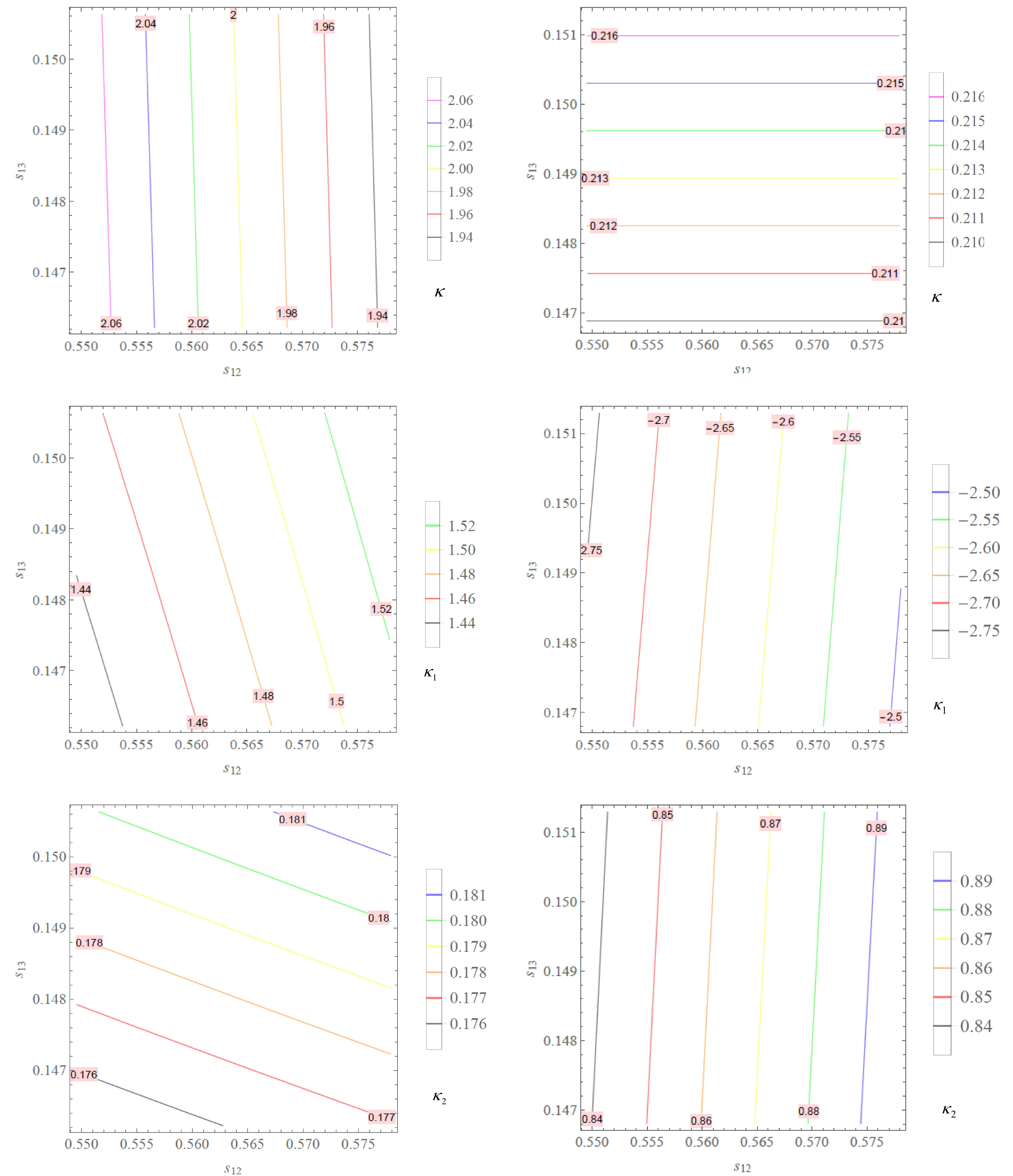
Figure 1. (color online)
$ \kappa $ and$ \kappa_{1,2} $ as functions of$ s_{12} $ and$ s_{13} $ with$ s_{12}\in (0.550, 0.578) $ and$ s_{13}\in (0.146, 0.151) $ for NH (left panel) and$ s_{13}\in (0.147, 0.151) $ for IH (right panel).
Figure 2. (color online)
$ \tau_{1,2} $ as functions of$ s_{12} $ and$ s_{13} $ with$ s_{12}\in (0.550, 0.578) $ and$ s_{13}\in (0.146, 0.151) $ for NH (left panel) and$ s_{13}\in (0.147, 0.151) $ for IH (right panel).$ \begin{aligned} &\kappa \in \left\{ \begin{array}{l} (1.94, 2.06) \; \;{\rm{for}}\;{\rm{NH}}, \\ (0.210, 0.216) \;\;{\rm{for}}\;{\rm{IH}}, \end{array} \right. \\&\kappa_1 \in \left\{ \begin{array}{l} (1.44, 1.52) \; \;{\rm{for}}\;{\rm{NH}}, \\ (-2.75, -2.50) \;\;{\rm{for}}\;{\rm{IH}}, \end{array} \right. \end{aligned} $

$ \begin{aligned}[b] &\kappa_2 \in \left\{ \begin{array}{l} (0.176, 0.181) \; \;{\rm{for}}\;{\rm{NH}}, \\ (0.84, 0.89) \;\;{\rm{for}}\;{\rm{IH}}, \end{array} \right. \\ &\tau_1 \in \left\{ \begin{array}{l} (1.93, 2.01) \; \;{\rm{for}}\;{\rm{NH}}, \\ (-1.59, -1.53) \; \;{\rm{for}}\;{\rm{IH}}, \end{array} \right. \,\, \\&\tau_2 \in \left\{ \begin{array}{l} (-0.655, -0.630) \; \;{\rm{for}}\;{\rm{NH}}, \\ (-0.822, -0.808) \; \;{\rm{for}}\;{\rm{IH}}. \end{array} \right. \end{aligned} $

(35) Expression (28) implies that
$ J_{\mathrm{CP}} $ depends on two parameters$ s_{12} $ and$ s_{13} $ , which is plotted in Fig. 3 with$ s_{12}\in (0.550, 0.578) $ and$ s_{13}\in (0.146, 0.151) $ for NH and$ s_{13}\in (0.147, 0.151) $ for IH. This shows that our model predicts a Jarlskog invariant range of$ J_{\mathrm{CP}} \in (-3.46, $ $ -3.30) 10^{-2} $ for NH and$ J_{\mathrm{CP}}\in (-3.48, -3.30) 10^{-2} $ for IH.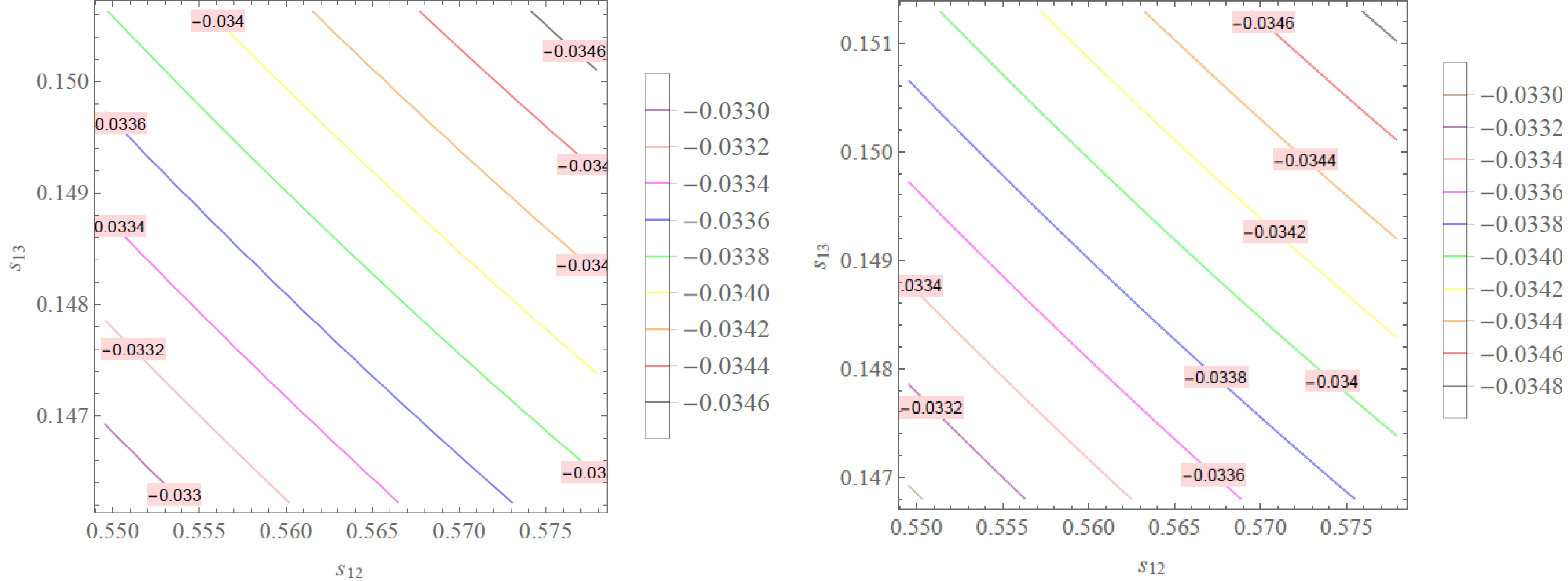
Figure 3. (color online)
$ J_{\mathrm{\rm CP}} $ as a function of$ s_{12} $ and$ s_{13} $ with$ s_{12}\in (0.550, 0.578) $ and$ s_{13}\in (0.146, 0.151) $ for NH (left panel) and$ s_{13}\in (0.147, 0.151) $ for IH (right panel).Expressions (30)-(32) show that
$ \alpha, \beta $ , and neutrino masses$ m_{2, 3} $ (NH),$ m_{1, 2} $ (IH) as well as the sum of neutrino masses$ \sum\nolimits_{\nu} m_\nu $ depend on$ \Delta m^2_{21} $ and$ \Delta m^2_{31} $ , which are plotted in Figs. 4, 5, and 6, respectively, within a$ 1\sigma $ range of the best-fit values taken from Ref. [1]. These are$ \Delta m^2_{21}\in (7.30, 7.72)\times 10^{-5} \,\mathrm{eV}^2 $ and$ \Delta m^2_{31}\in (2.52, 2.57) $ $ \times 10^{-3} \,\mathrm{eV}^2 $ for NH and$ \Delta m^2_{31}\in (-2.47, -2.42)\times 10^{-3} \,\mathrm{eV}^2 $ for IH. Figure 4 shows that the ranges of$ \alpha $ and$ \beta $ are as follows:
Figure 4. (color online)
$ \alpha $ and$ \beta $ as functions of$ \Delta m^2_{21} $ and$ \Delta m^2_{31} $ with$ \Delta m^2_{21}\in (7.30, 7.72)\times 10^{-5} \,\mathrm{eV}^2 $ and$ \Delta m^2_{31}\in (2.52, 2.57)\times 10^{-3} \,\mathrm{eV}^2 $ for NH (left panel) and$ \Delta m^2_{31}\in (-2.47, -2.42)\times 10^{-3} \,\mathrm{eV}^2 $ for IH (right panel).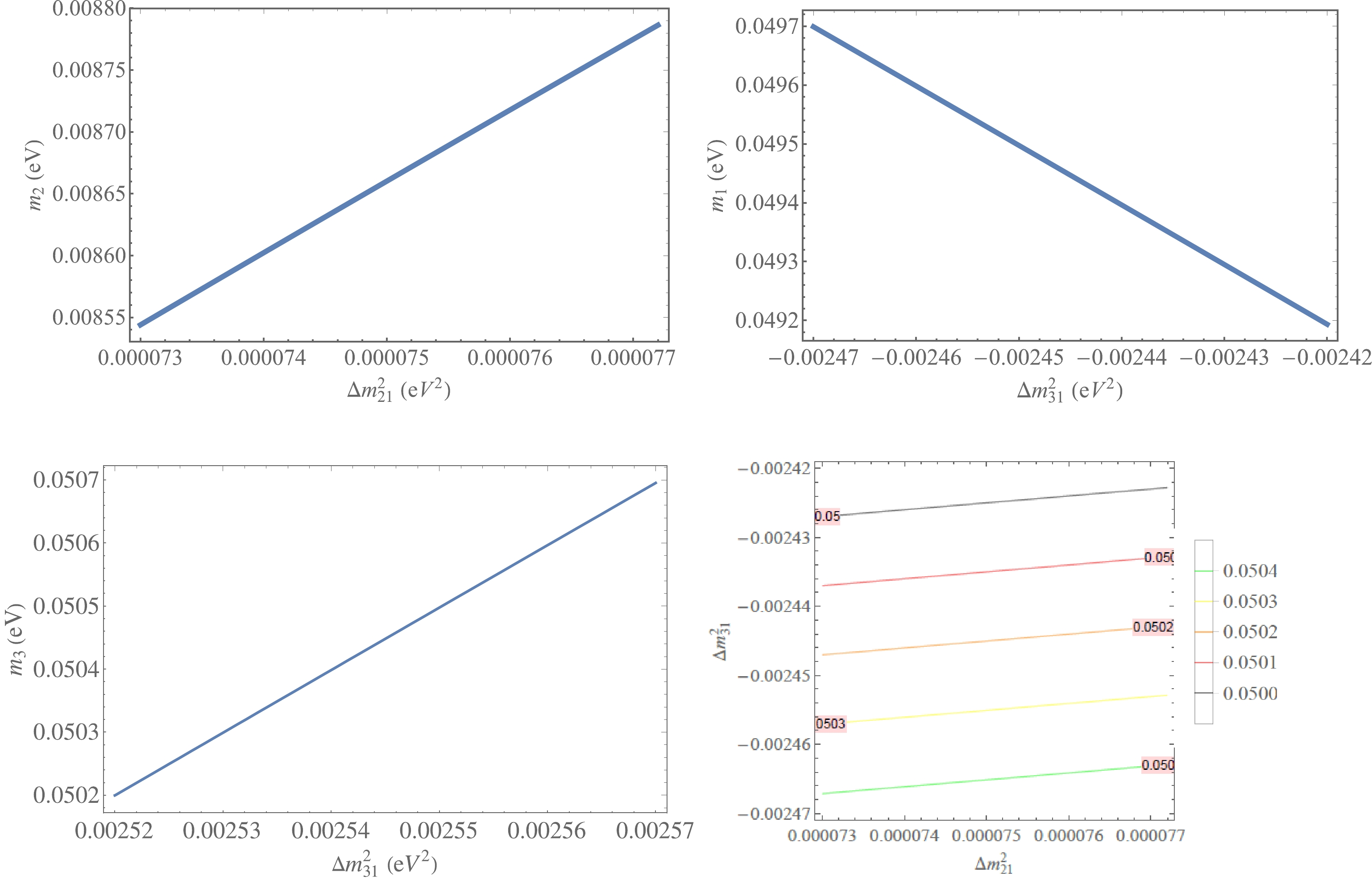
Figure 5. (color online)
$ m_{2}\, (m_3) $ as a function of$ \Delta m^2_{21} \, (\Delta m^2_{31}) $ for NH (left panel) and$ m_1 $ as a function of$ \Delta m^2_{31} $ and$ m_{2} $ as a function of$ \Delta m^2_{21} $ and$ \Delta m^2_{31} $ for IH (right panel) with$ \Delta m^2_{21}\in (7.30, 7.72)\times 10^{-5} \,\mathrm{eV}^2 $ and$ \Delta m^2_{31}\in (2.52, 2.57)\times 10^{-3} \,\mathrm{eV}^2 $ for NH and$ \Delta m^2_{31}\in (-2.47, -2.42)\times 10^{-3} \,\mathrm{eV}^2 $ for IH.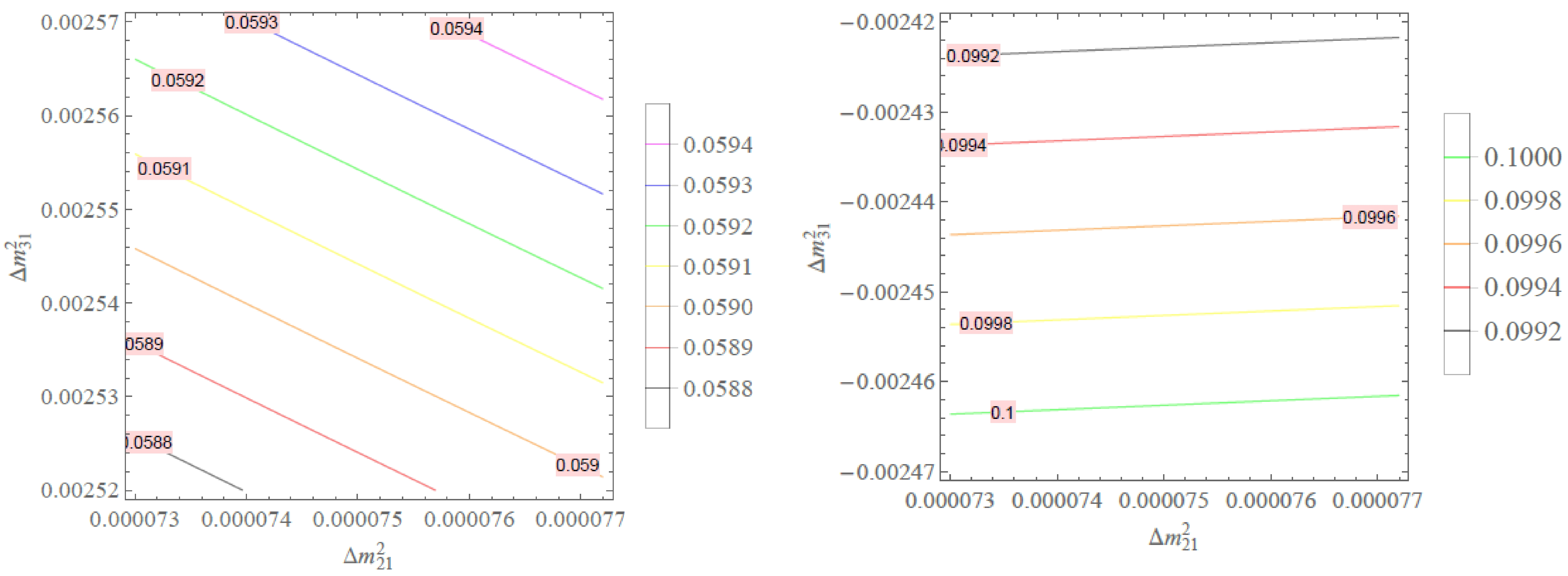
Figure 6. (color online)
$ \sum\nolimits_\nu m_{\nu} $ as a function of$ \Delta m^2_{21} $ and$ \Delta m^2_{31} $ with$ \Delta m^2_{21}\in (7.30, 7.72)\times 10^{-5} \,\mathrm{eV}^2 $ and$ \Delta m^2_{31}\in (2.52, 2.57)\times 10^{-3} \,\mathrm{eV}^2 $ for NH (left panel) and$ \Delta m^2_{31}\in (-2.47, -2.42)\times 10^{-3} \,\mathrm{eV}^2 $ for IH (right panel).$\alpha\in \left\{ \begin{array}{l} (-2.97, -2.94)\times 10^{-2}\, \mathrm{eV} \; \;{\rm{for}}\;{\rm{NH}}, \\ (-5.00, -4.96)\times 10^{-2}\, \mathrm{eV} \quad \,{\rm{for}}\;{\rm{IH}}, \end{array} \right. $

(36) $ \beta \in \left\{ \begin{array}{l} (2.075, 2.105)\times 10^{-2}\, \mathrm{eV} \; \;{\rm{for}}\;{\rm{NH}}, \\ (3.65, 3.88)\times 10^{-4}\, \mathrm{eV} \quad \,{\rm{for}}\;{\rm{IH}}. \end{array} \right. $

(37) Figure 5 shows that our model predicts the range of neutrino masses.
$ \left\{ \begin{array}{l} m_2 \in (8.55, 8.80)\times 10^{-3}\, \mathrm{eV},\\ m_3 \in (5.02, 5.07) \times 10^{-2} \, \mathrm{eV} \; \;{\rm{for}}\;{\rm{NH}}, \\ m_1 \in (4.92, 4.97)\times 10^{-2}\, \mathrm{eV},\\ m_2 \in (5.00, 5.04) \times 10^{-2} \, \mathrm{eV} \quad \,{\rm{for}}\;{\rm{IH}}. \end{array} \right. $

(38) Figure 6 shows that our model predicts the range of the sum of neutrino masses.
$\sum\limits_\nu m_\nu \in \left\{ \begin{array}{l} (5.88, 5.94)\times 10^{-2}\, \mathrm{eV} \; \;{\rm{for}}\;{\rm{NH}}, \\ (9.92\times 10^{-2}, 10^{-1}) \, \mathrm{eV} \quad \,{\rm{for}}\;{\rm{IH}}. \end{array} \right. $

(39) By taking the best-fit values of neutrino mass squared splittings for NH [1], as given in Table 1,
$ \Delta m^2_{21} = $ $ 7.50 \times 10^{-5} \, \mathrm{eV}^2, \Delta m^2_{31} = 2.55\times 10^{-3}\, \mathrm{eV}^2 $ , we obtain$\begin{aligned}[b]& \alpha = \left\{ \begin{array}{l} - 2.96\times 10^{-2}\, \mathrm{eV} \; \;{\rm{for}}\;{\rm{NH}}, \\ -4.99 \times 10^{-2} \, \mathrm{eV} \quad \,{\rm{for}}\;{\rm{IH}}, \end{array} \right. \\&\beta = \left\{ \begin{array}{l} 2.09\times 10^{-2}\, \mathrm{eV} \; \;{\rm{for}}\;{\rm{NH}}, \\ 3.76\times 10^{-4} \, \mathrm{eV} \quad \,{\rm{for}}\;{\rm{IH}}. \end{array} \right. \end{aligned}$

(40) These produce the following neutrino masses:
$ \left\{ \begin{array}{l} m_1 = 0, m_2 = 8.66\times 10^{-3}\, \mathrm{eV},\\ m_3 = 5.05\times 10^{-2}\, \mathrm{eV} \; \;{\rm{for}}\;{\rm{NH}}, \\ m_1 = 4.95 \times 10^{-2} \, \mathrm{eV}, m_2 = 5.02 \times 10^{-2} \, \mathrm{eV},\\ m_3 = 0 \;\;{\rm{for}}\;{\rm{IH}}. \end{array} \right.$

(41) The sum of the neutrino masses has the explicit values
$\sum m_{i = 1}^{3} = \left\{ \begin{array}{l} 5.92\times 10^{-2}\, \mathrm{eV} \; \;{\rm{for}}\;{\rm{NH}}, \\ 9.97 \times 10^{-2} \, \mathrm{eV} \;\;{\rm{for}}\;{\rm{IH}}. \end{array} \right. $

(42) At present, there are various bounds on
$ \sum m_{i} $ ; for instance, for NH, the upper limit on the sum of the neutrino masses is$ \sum m_i < 0.13\, \mathrm{eV} $ at a$ 2\, \sigma $ range [1], the strongest bound from cosmology [43] is$ \sum m_\nu < 0.078 \, \mathrm{eV} $ , the upper bound taken from [44] is$ \sum m_\nu < 0.12\div 0.69 \, \mathrm{eV} $ , and the constraint in Ref. [45] is$ \sum m_\nu <0.118\, \mathrm{eV} $ . For IH, the tightest$ 2 \sigma $ upper limit is$ \sum m_i < 0.15 \, \mathrm{eV} $ [1], and the upper limit taken from [46] is$ \sum m_\nu < 1.1\, \mathrm{eV} $ . Therefore, the prediction of our model in Eq. (39) is in good agreement.Expressions (33) and (34) imply that
$ m_{\beta } $ and$ \langle m_{ee}\rangle $ depend on four experimental parameters$ \Delta m_{21}^2, \Delta m_{31}^2, s_{12} $ , and$ s_{13} $ . At the best-fit points of the two neutrino mass-squared differences, two neutrino effective masses$ \langle m_{ee}\rangle $ and$ m_{\beta} $ depend on two parameters$ s_{12} $ and$ s_{13} $ , which is plotted in Fig. 7 with$ s_{12}\in (0.550, 0.578) $ and$ s_{13}\in (0.146, 0.151) $ for NH and$ s_{13}\in $ (0.147, 0.151) for IH. This shows that our model predicts the range of the effective neutrino mass parameters as follows: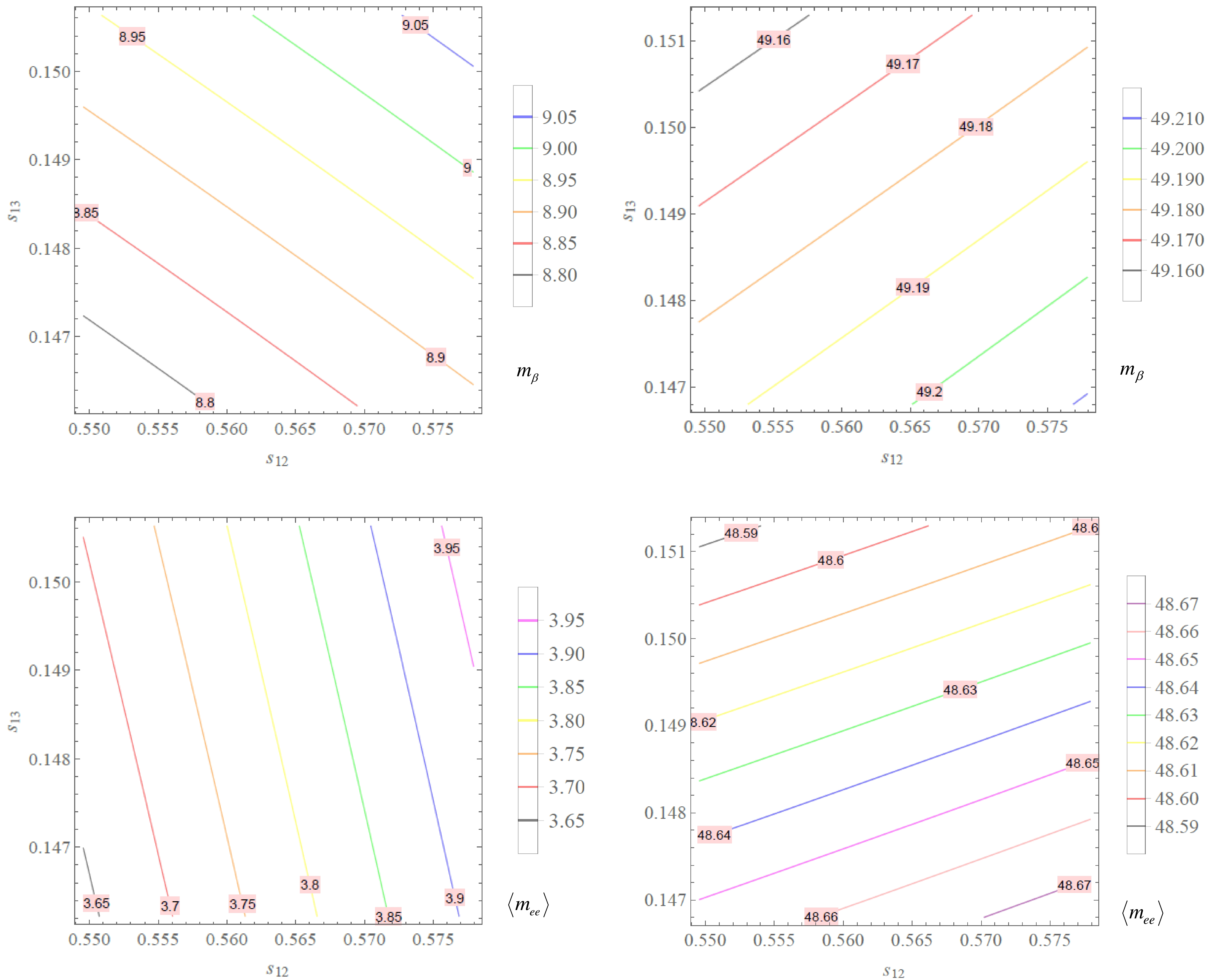
Figure 7. (color online)
$ m_{\beta} $ and$ \langle m_{ee}\rangle $ (in meV) as functions of$ s_{12} $ and$ s_{13} $ with$ s_{12}\in (0.550, 0.578) $ and$ s_{13}\in (0.146, 0.151) $ for NH (left panel) and$ s_{13}\in (0.147, 0.151) $ for IH (right panel).$ m_{\beta }\, (\mathrm{meV}) \in \left\{ \begin{array}{l} (8.80, 9.05) \; \;{\rm{for}}\;{\rm{NH}}, \\ (49.16, 49.21) \;\;{\rm{for}}\;{\rm{IH}}, \end{array}\right. $

(43) $ \langle m_{ee}\rangle \, (\mathrm{meV})\in \left\{ \begin{array}{l} (3.65, 3.95) \; \;{\rm{for}}\;{\rm{NH}}, \\ (48.59, 48.67) \;\;{\rm{for}}\;{\rm{IH}}. \end{array} \right. $

(44) At the best-fit points of
$ s_{12} $ and$ s_{13} $ taken from [1], as given in Table 1, we obtain$\begin{aligned}[b]& \kappa = \left\{ \begin{array}{l} 2.00 \; \;{\rm{for}}\;{\rm{NH}}, \\ 0.213 \;\;{\rm{for}}\;{\rm{IH}}, \end{array} \right. \quad \kappa_1 = \left\{ \begin{array}{l} \,\, 1.48 \; \;{\rm{for}}\;{\rm{NH}}, \\ -2.62 \;\;{\rm{for}}\;{\rm{IH}}, \end{array} \right.\\& \kappa_2 = \left\{ \begin{array}{l} 0.178 \; \;{\rm{for}}\;{\rm{NH}}, \\ 0.867 \;\;{\rm{for}}\;{\rm{IH}}, \end{array} \right. \quad \tau_1 = \left\{ \begin{array}{l} \,\,1.97 \; \;{\rm{for}}\;{\rm{NH}}, \\ -1.56 \; \;{\rm{for}}\;{\rm{IH}}, \end{array} \right.\\& \tau_2 = \left\{ \begin{array}{l} -0.643 \; \;{\rm{for}}\;{\rm{NH}}, \\ -0.815 \;\;{\rm{for}}\;{\rm{IH}}, \end{array} \right.\end{aligned} $

(45) $J_{\mathrm{CP}} = \left\{ \begin{array}{l} -3.38\times 10^{-2} \; \;{\rm{for}}\;{\rm{NH}}, \\ -3.40\times 10^{-2} \; \;{\rm{for}}\;{\rm{IH}}, \end{array} \right. $

(46) $\begin{aligned}[b] m_{\beta } = \left\{ \begin{array}{l} 8.91 \, \mathrm{meV} \; \;{\rm{for}}\;{\rm{NH}}, \\ 49.20 \,\mathrm{meV} \;\;{\rm{for}}\;{\rm{IH}}, \end{array} \right. \end{aligned}$

$\begin{aligned}[b]\langle m_{ee}\rangle = \left\{ \begin{array}{l} 3.80 \, \mathrm{meV} \; \;{\rm{for}}\;{\rm{NH}}, \\ 48.60 \, \mathrm{meV} \; \;{\rm{for}}\;{\rm{IH}}. \end{array} \right. \end{aligned}$

(47) The corresponding mixing matrices are
${U_{{\rm{Lep}}}} = \left\{ {\begin{array}{*{20}{l}} {\left( {\begin{array}{*{20}{c}} {0.817}&{0.558}&{0.148}\\ {0.289 + 0.289i}&{ - 0.266 - 0.523i}&{ - 0.588 + 0.378i}\\ { - 0.289 + 0.289i}&{0.266 - 0.523i}&{0.588 + 0.378i} \end{array}} \right)\; \;{\rm{for}}\;{\rm{NH}},}\\ {\left( {\begin{array}{*{20}{c}} { - 0.817}&{0.558}&{0.149}\\ { - 0.220 + 0.344i}&{ - 0.445 + 0.371i}&{0.494 + 0.494i}\\ {0.220 + 0.344i}&{0.445 + 0.371i}&{ - 0.494 + 0.494i} \end{array}} \right)\; \;{\rm{for}}\;{\rm{IH}},} \end{array}} \right.$ 
(48) which are unitary and in good agreement with the entry constraint of the lepton mixing matrix in Ref. [47].
Global data analyses [44, 47] show that
$ \delta_{CP} $ is close to$ -\dfrac{\pi}{2} $ , and the best fit value of$\delta_{\rm CP}$ in [47, 48] is close to$ -\dfrac{\pi}{2} $ for both NH and IH. For$\delta_{\rm CP}$ and$ \theta_{23} $ , as shown in Eq. (26), our model predicts$\delta_{\rm CP} = -\dfrac{\pi}{2}$ and$ \theta_{23} = \dfrac{\pi}{4} $ , respectively, which are consistent with the cobimaximal mixing pattern and within the$ 3\sigma $ range of the best-fit values taken from Ref. [1]. The resulting effective neutrino mass parameters in Eq. (47) are below the upper bound arising from present$ 0\nu \beta \beta $ decay experiments; however, they are highly consistent with the future large and ultra-low background liquid scintillator detectors, which have been discussed in Ref. [49]. The$ \mathrm{meV} $ limit of the effective neutrino mass can be reached by planning future experiments [43, 50-56]. -
We have constructed a non-renormalizable gauge
$ B-L $ model based on$ Q_4\times Z_4\times Z_2 $ symmetry that leads to the successful cobimaximal lepton mixing scheme. Small active neutrino masses and both neutrino mass hierarchies are produced via the type-I seesaw mechanism at the tree-level. The model is predictive; hence, it reproduces the cobimaximal lepton mixing scheme, and the reactor neutrino mixing angle$ \theta_{13} $ and the solar neutrino mixing angle$ \theta_{12} $ can obtain best-fit values from recent experimental data. Our model also predicts the effective neutrino mass parameters of$ m_{\beta }\in (8.80, 9.05)\, \mathrm{meV} $ and$ \langle m_{ee}\rangle \in (3.65, 3.95)\, \mathrm{meV} $ for normal ordering (NO) and$ m_{\beta }\in (49.16, 49.21)\, \mathrm{meV} $ and$ \langle m_{ee}\rangle \in (48.59, 48.67)\, \mathrm{meV} $ for inverted ordering (IO), which are highly consistent with recent experimental constraints. -
The total scalar potential invariant under all of the model's symmetries is given by①
$\tag{A1} \begin{aligned}[b] \mathbf{V}_{\mathrm{total}}= & V(H)+V(\chi)+V(\rho)+V(\eta)+ V(\phi)+V(\varphi) + V(H, \chi)+V(H, \rho)+V(H, \eta)+ V(H, \phi)+V(H, \varphi) \\& +V(\chi, \rho)+V(\chi, \eta)+ V(\chi, \phi)+V(\chi, \varphi)+ V(\rho, \eta) + V(\rho, \phi)+V(\rho, \varphi)+ V(\eta, \phi)+V(\eta, \varphi)+ V(\phi, \varphi) + V_{\mathrm{multiple}}, \end{aligned} $ 
where②
$\tag{A2}V(H) = \mu_{H}^2 (H^\dagger H)_{\mathbf{1}_1} +\lambda^{H} ({H}^\dagger H)_{\mathbf{1}_1}({H}^\dagger H)_{\mathbf{1}_1}, $

$\tag{A3} V(\chi) = \mu_{\chi}^2 \chi^2 +\lambda^{\chi}_1 \chi^4+\lambda^{\chi}_2 (\chi^*\chi)_{\mathbf{1}_2}(\chi^*\chi)_{\mathbf{1}_2}, V(\rho) = V(\chi\rightarrow \rho),$

$\tag{A4} V(\eta) = \mu_{\eta}^2 (\eta^*\eta)_{\mathbf{1}_1} +\lambda^{\eta}_1 (\eta \eta)_{\mathbf{1}_3} (\eta \eta)_{\mathbf{1}_3} +\lambda^{\eta}_2 (\eta\eta)_{\mathbf{1}_4} (\eta \eta)_{\mathbf{1}_4}+\lambda^{\eta}_3 (\eta^*\eta)_{\mathbf{1}_1} (\eta^*\eta)_{\mathbf{1}_1}+\lambda^{\eta}_4 (\eta^*\eta)_{\mathbf{1}_2} (\eta^*\eta)_{\mathbf{1}_2}, $

$\tag{A5} \begin{aligned}[b] V(\phi) =& \mu_{\phi}^2 (\phi^* \phi)_{\mathbf{1}_1} + \lambda^{\phi} ({\phi}^*\phi)_{\mathbf{1}_1}({\phi}^*\phi)_{\mathbf{1}_1}, V(\varphi) = V(\phi \rightarrow \varphi), V(H, \chi) = \lambda^{H \chi}_1 ({H}^\dagger H)_{\mathbf{1}_1}(\chi^2)_{\mathbf{1}_1} \\ & + \lambda^{H\chi}_2 ({H}^\dagger \chi)_{\mathbf{1}_3}({\chi} H)_{\mathbf{1}_3}, V(H, \rho) = \lambda^{H \rho}_1 ({H}^\dagger H)_{\mathbf{1}_1}(\rho^2)_{\mathbf{1}_1}+ \lambda^{H\rho}_2 ({H}^\dagger \rho)_{\mathbf{1}_4}({\rho} H)_{\mathbf{1}_4}, \end{aligned} $

$\tag{A6}\begin{aligned}[b] V(H, \eta) =& \lambda^{H \eta}_1 ({H}^\dagger H)_{\mathbf{1}_1}({\eta}^*\eta)_{\mathbf{1}_1} + \lambda^{H\eta}_2 ({H}^\dagger \eta)_{\mathbf{2}}({\eta}^* H)_{\mathbf{2}}, V(H, \phi) = \lambda^{H \phi}_1 ({H}^\dagger H)_{\mathbf{1}_1}({\phi}^*\phi)_{\mathbf{1}_1} \\ & + \lambda^{H\phi}_2 ({H}^\dagger \phi)_{\mathbf{1}_1}({\phi}^* H)_{\mathbf{1}_1}, V(H, \varphi) = \lambda^{H \varphi}_1 ({H}^\dagger H)_{\mathbf{1}_1}({\varphi}^*\varphi)_{\mathbf{1}_1} + \lambda^{H\varphi}_2 ({H}^\dagger \varphi)_{\mathbf{1}_2}({\varphi}^* H)_{\mathbf{1}_2}, \end{aligned} $

$\tag{A7}V(\chi,\rho) = \lambda^{\chi \rho}_1 {\chi}^2\rho^2 + \lambda^{\chi\rho}_2 ({\chi}\rho)_{\mathbf{1}_2}(\rho{\chi})_{\mathbf{1}_2} + \lambda^{\chi\rho}_3 ({\chi}^*\chi)_{\mathbf{1}_2}(\rho^*{\rho})_{\mathbf{1}_2} + \lambda^{\chi\rho}_4 ({\chi}^*\rho)_{\mathbf{1}_1}(\rho^*{\chi})_{\mathbf{1}_1}, $

$\tag{A8} V(\chi,\eta) = \lambda^{\chi \eta}_1 {\chi}^2(\eta^*\eta)_{\mathbf{1}_1} + \lambda^{\chi\eta}_2 ({\chi^*}\chi)_{\mathbf{1}_2}(\eta^* \eta)_{\mathbf{1}_2} + \lambda^{\chi\eta}_3 ({\chi}\eta^*)_{\mathbf{2}}(\eta \chi)_{\mathbf{2}} + \lambda^{\chi\eta}_4 ({\chi}^*\eta)_{\mathbf{2}}(\eta^*{\chi})_{\mathbf{2}}, $

$\tag{A9} V(\chi, \phi) = \lambda^{\chi \phi}_1 {\chi}^2 (\phi^*\phi)_{\mathbf{1}_1} + \lambda^{\chi\phi}_2 (\chi \phi)_{\mathbf{1}_3}(\phi^* \chi)_{\mathbf{1}_3},\, V(\chi, \varphi) = \lambda^{\chi \varphi}_1 {\chi}^2 (\varphi^*\varphi)_{\mathbf{1}_1} + \lambda^{\chi\varphi}_2 (\chi \varphi)_{\mathbf{1}_4}(\varphi^* \chi)_{\mathbf{1}_4}, $

$\tag{A10} V(\rho,\eta) = \lambda^{\rho \eta}_1 {\rho}^2(\eta^*\eta)_{\mathbf{1}_1} + \lambda^{\rho\eta}_2 ({\rho^*}\rho)_{\mathbf{1}_2}(\eta^* \eta)_{\mathbf{1}_2} + \lambda^{\rho\eta}_3 ({\rho}\eta^*)_{\mathbf{2}}(\eta \rho)_{\mathbf{2}} + \lambda^{\rho\eta}_4 ({\rho}^*\eta)_{\mathbf{2}}(\eta^*{\rho})_{\mathbf{2}}, $

$\tag{A11} V(\rho, \phi) = \lambda^{\rho \phi}_1 {\rho}^2 (\phi^*\phi)_{\mathbf{1}_1} + \lambda^{\rho\phi}_2 (\rho \phi)_{\mathbf{1}_4}(\phi^* \rho)_{\mathbf{1}_4},\, V(\rho, \varphi) = \lambda^{\rho \varphi}_1 {\rho}^2 (\varphi^*\varphi)_{\mathbf{1}_1} + \lambda^{\rho\varphi}_2 (\rho \varphi)_{\mathbf{1}_3}(\varphi^* \rho)_{\mathbf{1}_3}, $

$\tag{A12} V(\eta, \phi) = \lambda^{\eta \phi}_1 (\eta^* \eta)_{\mathbf{1}_1}(\phi^*\phi)_{\mathbf{1}_1} + \lambda^{\eta\phi}_2 (\eta^* \phi)_{\mathbf{2}}(\phi^* \eta)_{\mathbf{2}}, V(\eta, \varphi) = V(\eta, \phi\rightarrow \varphi), $

$\tag{A13} V(\phi, \varphi) = \lambda^{\phi \varphi}_1 (\phi^* \phi)_{\mathbf{1}_1}(\varphi^*\varphi)_{\mathbf{1}_1} + \lambda^{\phi\varphi}_2 (\phi^* \varphi)_{\mathbf{1}_2}(\varphi^* \phi)_{\mathbf{1}_2}, V_{\mathrm{multiple}} = 0. $

All the other terms with three or more different scalars are forbidden by one or some of the model's symmetries. For cubic couplings, ten couplings of H and two different scalars in the set of
$ \{\chi, \rho, \eta, \phi, \varphi \} $ are prevented by the$ U(1)_Y $ symmetry; four couplings$ \chi \rho\eta, \chi\phi\varphi, \rho\phi^*\varphi $ and$ \eta\phi^*\varphi $ are forbidden by the$ Q_4 $ symmetry; and six couplings$ \chi\rho\phi, \chi\rho\varphi, \chi\eta\phi, \chi\eta\varphi, \rho\eta\phi $ and$ \rho\eta\varphi $ are prevented by the$ U(1)_{B-L} $ symmetry. For quartic couplings, ten couplings of H and three different scalars in the set of$ \{\chi, \rho, \eta, \phi, \varphi \} $ are prevented by the$ U(1)_Y $ symmetry; four couplings$ \chi \rho\eta\phi, \chi \rho\eta\varphi,\chi\eta\phi\varphi $ , and$ \rho\eta\phi\varphi $ are forbidden by the$ Q_4 $ symmetry; and the coupling$ \chi\rho\phi^*\varphi $ is prevented by the$ Z_2 $ symmetry. For quintic couplings, five couplings of H and four different scalars in the set of$ \{\chi, \rho, \eta, \phi, \varphi \} $ are prevented by the$ U(1)_Y $ symmetry; the coupling$ \chi \rho\eta\phi^*\varphi $ is forbidden by the$ Q_4 $ symmetry; and$ H^+H \phi^*\varphi\chi $ and$ H^+H \phi^*\varphi\rho $ are prevented by the$ Q_4 $ symmetry.To show that the scalar fields with the VEV alignments in Eq. (1) are natural solutions of the minimum condition of
$ V_{\mathrm{scalar}} $ in Eqs. (A1)-(A13), we put$ v^*_{H} = v_{H}, \,v^*_\chi = v_\chi, \,v^*_\rho = v_\rho, \,v_{\eta_1} = v_{\eta_2} = v_{\eta}, \,v^*_\eta = v_\eta,\, v^*_\phi = v_\phi $ and$ v^*_\varphi = v_\varphi $ , which leads to$ \dfrac{\partial V_{\mathrm{scalar}}}{\partial v^*_j} = \dfrac{V_{\mathrm{scalar}}}{\partial v_j}, \dfrac{\partial^2 V_{\mathrm{scalar}}}{\partial v^{*2}_j} = $ $ \dfrac{V_{\mathrm{scalar}}}{\partial v^2_j} \,\, (v_j = v_H, v_\chi, v_\rho, v_\eta, v_\phi, v_\varphi) $ , and the minimization condition of$ V_{\mathrm{scalar}} $ reduces to$ \tag{A14} \frac{\partial V_{\mathrm{scalar}}}{\partial v_j} =0, \frac{\partial^2 V_{\mathrm{scalar}}}{\partial v^2_j} >0. $

For simplicity, we use the following notations:
$\tag{A15} \begin{aligned}[b] &\lambda^{\chi} = \lambda^{\chi} _1 +\lambda^{\chi}_2, \lambda^{\rho} = \lambda^{\rho}_1 +\lambda^{\rho}_2, \lambda^{\eta} = \sum\limits_{k = 1}^4 \lambda^{\eta}_k, \lambda^{H\chi} = \lambda^{H\chi}_1 + \lambda^{H\chi}_2, \lambda^{\chi\rho} = \sum\limits_{k = 1}^4 \lambda^{\chi\rho}_k, \\ &\lambda^{H\rho} = \lambda^{H\rho}_1 + \lambda^{H\rho}_2, \lambda^{H\eta} = \lambda^{H\eta}_2-\lambda^{H\eta}_1, \lambda^{H\phi} = \lambda^{H\phi}_1 + \lambda^{H\phi}_2, \lambda^{H\varphi} = \lambda^{H\varphi}_1 + \lambda^{H\varphi}_2, \\ &\lambda^{\chi\eta} = \lambda^{\chi\eta}_1 +\lambda^{\chi\eta}_2+ \lambda^{\chi\eta}_3 -\lambda^{\chi\eta}_4, \lambda^{\chi\phi} = \lambda^{\chi\phi}_1+\lambda^{\chi\phi}_2, \lambda^{\chi\varphi} = \lambda^{\chi\varphi}_1 +\lambda^{\chi\varphi}_2, \\ &\lambda^{\rho\eta} = \lambda^{\rho\eta}_1+ \lambda^{\rho\eta}_2 +\lambda^{\rho\eta}_3-\lambda^{\rho\eta}_4, \lambda^{\rho\phi} = \lambda^{\rho\phi}_1 +\lambda^{\rho\phi}_2, \lambda^{\rho\varphi} = \lambda^{\rho\varphi}_1 +\lambda^{\rho\varphi}_2, \\ &\lambda^{\eta\varphi} = \lambda^{\eta\varphi}_1 +\lambda^{\eta\varphi}_2, \lambda^{\eta\phi} = \lambda^{\eta\phi}_1 +\lambda^{\eta\phi}_2, \lambda^{\phi\varphi} = \lambda^{\phi\varphi}_1 +\lambda^{\phi\varphi}_2. \\\end{aligned} $ 
Thus, the minimization conditions in Eq. (A14) reduce to
$\tag{A16} \mu_{H}^2 + 2\lambda^{H\varphi} v_\varphi^2 + \lambda^{H\chi}v_\chi^2 + 2\lambda^{H\eta}v_\eta^2 + 2 \lambda^{H} v_H^2 + \lambda^{H\phi}v_\phi^2 + \lambda^{H\rho}v_\rho^2 = 0, $

$ \tag{A17}\mu_{\chi}^2 + \lambda^{\chi\varphi} v_\varphi^2 + 2\lambda^{\chi}v_\chi^2 - 2\lambda^{\chi\eta}v_\eta^2 + \lambda^{H\chi}v_H^2 + \lambda^{\chi\phi}v_\phi^2 + \lambda^{\chi\rho}v_\rho^2 = 0, $

$\tag{A18} \mu_{\rho}^2 + \lambda^{\rho\varphi}v_\varphi^2 + \lambda^{\chi\rho}v_\chi^2 - 2\lambda^{\rho\eta}v_\eta^2 + \lambda^{H\rho}v_H^2 + \lambda^{\rho\phi}v_\phi^2 + 2\lambda^{\rho}v_\rho^2 = 0, $

$\tag{A19} 2 \mu_{\eta}^2 + 2 (\lambda^{\eta\varphi} v_\varphi^2 + \lambda^{\chi\eta}v_\chi^2 - 4\lambda^{\eta}v_\eta^2 - \lambda^{H\eta}v_H^2 + \lambda^{\eta\phi}v_\phi^2) + 2\lambda^{\rho\eta}v_\rho^2 = 0, $

$ \tag{A20}\mu_{\phi}^2 + \lambda^{\phi\varphi}v_\varphi^2 + \lambda^{\chi\phi}v_\chi^2 - 2\lambda^{\eta\phi}v_\eta^2 + \lambda^{H\phi}v_H^2 + 2 \lambda^{\phi} v_\phi^2 + \lambda^{\rho\phi}v_\rho^2 = 0, $

$ \tag{A21}\mu_{\varphi}^2 + 2 \lambda^{\varphi} v_\varphi^2 + \lambda^{\chi\varphi}v_\chi^2 - 2\lambda^{\eta\varphi}v_\eta^2 + 2\lambda^{H\varphi}v_H^2 + \lambda^{\phi\varphi}v_\phi^2 + \lambda^{\rho\varphi}v_\rho^2 = 0, $

$\tag{A22} \mu_{H}^2 + 2\lambda^{H\varphi}v_\varphi^2 + \lambda^{H\chi}v_\chi^2 + 2\lambda^{H\eta}v_\eta^2 + 6 \lambda^{H} v_H^2 + \lambda^{H\phi}v_\phi^2 + \lambda^{H\rho}v_\rho^2 >0, $

$\tag{A23} \mu_{\chi}^2 + \lambda^{\chi\varphi}v_\varphi^2 + 6\lambda^{\chi}v_\chi^2 - 2\lambda^{\chi\eta}v_\eta^2 + \lambda^{H\chi}v_H^2 + \lambda^{\chi\phi}v_\phi^2 + \lambda^{\chi\rho}v_\rho^2>0, $

$\tag{A24} \mu_{\rho}^2 + \lambda^{\rho\varphi}v_\varphi^2 + \lambda^{\chi\rho}v_\chi^2 - 2\lambda^{\rho\eta}v_\eta^2 + \lambda^{H\rho}v_H^2 + \lambda^{\rho\phi}v_\phi^2 + 6\lambda^{\rho}v_\rho^2 > 0, $

$\tag{A25} -2 \mu_{\eta}^2 - 2 (\lambda^{\eta\varphi}v_\varphi^2 + \lambda^{\chi\eta}v_\chi^2 - 12\lambda^{\eta}v_\eta^2 -\lambda^{H\eta}v_H^2 + \lambda^{\eta\phi}v_\phi^2) - 2\lambda^{\rho\eta} v_\rho^2>0, $

$\tag{A26} \mu_{\phi}^2 + \lambda^{\phi\varphi}v_\varphi^2 + \lambda^{\chi\phi}v_\chi^2 - 2\lambda^{\eta\phi}v_\eta^2 + \lambda^{H\phi} v_H^2 + 6 \lambda^{\phi} v_\phi^2 + \lambda^{\rho\phi}v_\rho^2> 0, $

$\tag{A27} \mu_{\varphi}^2 + 6 \lambda^{\varphi} v_\varphi^2 + \lambda^{\chi\varphi}v_\chi^2 - 2\lambda^{\eta\varphi}v_\eta^2 + 2\lambda^{H\varphi}v_H^2 + \lambda^{\phi\varphi}v_\phi^2 + \lambda^{\rho\varphi}v_\rho^2 > 0. $

The system of Eqs. (A16)–(A21) always have the following solutions:
$\tag{A28} \lambda^{H} = -\left(\lambda^{H\chi} v_\chi^2+2 \lambda^{H\eta} v_\eta^2+\lambda^{H\phi} v_\phi^2+\lambda^{H\rho} v_\rho^2+2 \lambda^{H\varphi} v_\varphi^2+\mu_{H}^2\right)/(2 v_H^2), $

$\tag{A29} \lambda^{\chi} = -\left(\mu_{\chi}^2 + \lambda^{\chi\varphi} v_\varphi^2 - 2 \lambda^{\chi\eta} v_\eta^2 + \lambda^{H\chi} v_H^2 + \lambda^{\chi\phi} v_\phi^2 + \lambda^{\chi\rho} v_\rho^2\right)/(2 v_\chi^2), $

$\tag{A30} \lambda^{\rho} = -\left(\mu_{\rho}^2 + \lambda^{\rho\varphi} v_\varphi^2 + \lambda^{\chi\rho} v_\chi^2 - 2 \lambda^{\rho\eta} v_\eta^2 +\lambda^{H\rho} v_H^2 + \lambda^{\rho\phi} v_\phi^2\right)/(2 v_\rho^2), $

$\tag{A31} \lambda^{\eta} = \left(\mu_{\eta}^2 + \lambda^{\eta\varphi} v_\varphi^2 + \lambda^{\chi\eta} v_\chi^2 - \lambda^{H\eta} v_H^2 + \lambda^{\eta\phi} v_\phi^2 + \lambda^{\rho\eta} v_\rho^2\right)/(4 v_\eta^2), $

$\tag{A32} \lambda^{\phi} = -\left(\mu_{\phi}^2 + \lambda^{\phi\varphi} v_\varphi^2 + \lambda^{\chi\phi} v_\chi^2 - 2 \lambda^{\eta\phi} v_\eta^2 + \lambda^{H\phi} v_H^2 + \lambda^{\rho\phi} v_\rho^2\right)/(2 v_\phi^2), $

$\tag{A33} \lambda^{\varphi} = -\left(\mu_{\varphi}^2 + \lambda^{\chi\varphi} v_\chi^2 - 2 \lambda^{\eta\varphi} v_\eta^2 + 2 \lambda^{H\varphi} v_H^2 + \lambda^{\phi\varphi} v_\phi^2 + \lambda^{\rho\varphi} v_\rho^2\right)/(2 v_\varphi^2). $

Next, with
$ \lambda^{H}, \lambda^{\chi}, \lambda^{\rho}, \lambda^{\eta}, \lambda^{\phi} $ , and$ \lambda_{\varphi} $ in Eqs. (A28)–(A33), there exist possible regions of the model's parameters such that the inequalities (A22)–(A27) are always satisfied by the solution, as shown in Eq. (1). For instance, with the benchmark point$\tag{A34} v_H \simeq v_\chi \simeq v_\rho \simeq v_\eta \simeq 10^{11}\, \mathrm{eV}, v_\varphi \simeq v_\phi = 10^{12}\, \mathrm{eV}, $

$ \tag{A35}\mu_H^2 \simeq \mu_\chi^2\simeq \mu_\rho^2\simeq \mu_\eta^2 \simeq \mu_\phi^2 \simeq \mu_{\varphi}^2 = -10^{16} \, \mathrm{eV}^2,$

$\tag{A36} \begin{aligned}[b] \lambda^{\chi\eta} =& \lambda^{\rho\eta} = \lambda^{\eta\phi} = \lambda^{\eta\varphi} = -\lambda^{\rho\varphi} = -\lambda^{H\chi} = -\lambda^{H\eta}\\=& - \lambda^{H\rho} = -\lambda^{H\phi} = - \lambda^{H\varphi} = -\lambda^{\rho\phi} = -\lambda^{\chi\phi}\\ =& -\lambda^{\chi\rho} = -\lambda^{\chi\varphi} = \lambda_{0}, \end{aligned} $

the expressions in (A22)–(A27) are always satisfied in the case of
$ \lambda_{0} \in (10^{-4}, 10^{-2}) $ , which is shown in Fig. A1. Therefore, the VEVs in Eq. (1) are natural solutions of the potential minimum condition.
A non-renormalizable B-L model with Q4 × Z4 × Z2 flavor symmetry for cobimaximal neutrino mixing
- Received Date: 2021-08-13
- Available Online: 2021-12-15
Abstract: We construct a non-renormalizable gauge


 DownLoad: