Dark matter interactions from an extra U(1) gauge symmetry with kinetic mixing and Higgs charge

The standard model (SM) with ${S U}(3)_{C} \times {S U}(2)_{L} \times {U}(1)_{Y}$ gauge interactions has achieved significant success in explaining experimental data in particle physics. Nonetheless, the SM must be extended to take into account dark matter (DM) in the Universe, whose existence has been established by astrophysical and cosmological experiments [1−4]. The standard paradigm for DM production assumes that DM was thermally produced in the early Universe, typically requiring several mediators to induce adequate DM interactions with SM particles.

A simple strategy is to assume that the DM particle carries a ${{U}}(1)_{{X}}$ charge associated with an additional ${{U}}(1)_{{X}}$ gauge symmetry, with the corresponding gauge boson acting as a mediator [5]. To minimize the impact on the interactions of SM particles, one may assume that no SM field carries ${{U}}(1)_{{X}}$ charge [6−30]. Thus, the kinetic mixing between the ${{U}}(1)_{{X}}$ and ${{U}}(1)_{{Y}}$ gauge fields [31, 32] induces DM interactions with SM particles. Such a kinetic mixing portal is able to achieve the observed DM relic abundance via the freeze-out mechanism [33−35] and satisfy the constraints from DM direct detection experiments. A comprehensive study in Ref. [19] shows that there are various viable parameter windows for Dirac or Majorana fermionic DM, and several of them are promising for the LHC phenomenology or the interpretation of the Galactic Center gamma-ray excess.

Nevertheless, it is interesting to explore more possibilities beyond the simple kinetic mixing portal, and a larger parameter space may be helpful to satisfy the increasingly severe phenomenological constraints. In this study, we assume that the SM Higgs field also carries a ${{U}}(1)_{{X}}$ charge [36], which is very small to keep the new $Z^\prime$ gauge boson weakly coupled to the SM sector. Because of the kinetic mixing term and Higgs ${{U}}(1)_{{X}}$ charge, the ${{U}}(1)_{{X}}$ and ${{U}}(1)_{{Y}}$ gauge fields mix with each other, and one electrically neutral gauge boson, namely, a photon, remains massless. To ensure the gauge invariance of the SM Yukawa couplings, SM fermions should also be charged under ${{U}}(1)_{{X}}$. To cancel chiral gauge anomalies, we assume that the fermions carry Y-sequential ${{U}}(1)_{{X}}$ charges [36−40], which are also very small because they must be proportional to the Higgs ${{U}}(1)_{{X}}$ charge. Such a case is different from those conventionally proposed [12, 39, 41−45] because the latter usually have ${\cal O}(1)$ charges to lift physical processes. It is also notable that this case is similar to that for the U-boson [46, 47], in the sense that the ${{U}}(1)_{{X}}$ gauge couplings to SM particles are considerably weaker than those to DM. Now, there is one more free parameter, that is, the Higgs ${{U}}(1)_{{X}}$ charge, that affects the $Z^\prime$ couplings to SM particles. It is necessary to investigate its impact on DM phenomenology.

In this context, we study a Dirac fermionic DM particle [8, 10, 21, 23] and find that the DM couplings to protons and neutrons are typically different [9, 10, 12, 13, 17, 18], leading to isospin-violating DM-nucleon scattering [48] in direct detection experiments. It is not obvious whether the correct DM relic abundance can be achieved until we perform numerical scans. We find that the presence of the extra parameter can accommodate wider ranges of the ${{U}}(1)_{{X}}$ gauge coupling and DM particle mass.

This paper is organized as follows. In Sec. II, we introduce ${{U}}(1)_{{X}}$ gauge theory, where the Higgs doublet carries a ${{U}}(1)_{{X}}$ charge, and discuss the induced interactions of SM fermions. In Sec. III, we study Dirac fermionic DM charged under ${{U}}(1)_{{X}}$ and explore the effective DM-nucleon scattering cross-section for direct detection and the DM relic abundance via numerical scans. Finally, we present the conclusions in Sec. IV.

In this section, we introduce ${{U}}(1)_{{X}}$ gauge theory with kinetic mixing between the ${{U}}(1)_{{X}}$ and ${{U}}(1)_{{Y}}$ gauge fields. We assign a small ${{U}}(1)_{{X}}$ charge to the SM Higgs doublet, and the SM Yukawa interactions are gauge-invariant only if the SM fermions have appropriate ${{U}}(1)_{{X}}$ charges, which are chosen to be Y-sequential, that is, obey the same relations as their ${{U}}(1)_{{Y}}$ charges, so that the theory remains free from chiral anomalies.

We denote the ${{U}}(1)_{{Y}}$ and ${{U}}(1)_{{X}}$ gauge fields as $\hat{B}_\mu$ and $\hat{Z}'_\mu$, respectively. Their gauge-invariant kinetic terms in the Lagrangian read as

where the field strengths are $\hat{B}_{\mu\nu} \equiv \partial_\mu \hat{B}_\nu - \partial_\nu \hat{B}_\mu$ and $\hat{Z}'_{\mu\nu} \equiv \partial_\mu \hat{Z}'_\nu - \partial_\nu \hat{Z}'_\mu$. The $\sin\epsilon$ term is a kinetic mixing term, which gives the kinetic Lagrangian (1) a noncanonical form.

We assume that the ${{U}}(1)_{{X}}$ gauge symmetry is spontaneously broken [49−51] by a Higgs field $\hat{S}$ with ${{U}}(1)_{{X}}$ charge $x_S = 1$ ¹. Now, the Higgs sector involves $\hat{S}$ and the SM Higgs doublet $\hat{H}$. The corresponding Lagrangian with respect to the ${S U}(2)_{L} \times {U}(1)_{Y} \times {U}(1)_{X}$ gauge symmetry is [21]

The covariant derivatives are given by

where $W^a_\mu$ ($a=1,2,3$) denote the ${S U}(2)_{L}$ gauge fields, $T^a = \sigma^a/2$ are the ${S U}(2)_{L}$ generators. $\hat{g}$, $\hat{g}'$, and $g_X$ are the ${S U}(2)_{L}$, ${{U}}(1)_{{Y}}$, and ${{U}}(1)_{{X}}$ gauge couplings, respectively. The hypercharge $Y_H = 1/2$ for $\hat{H}$ is the same as in the SM.

The presence of the ζ term is notable here. They generally reflect the ${{U}}(1)_{{X}}$ charge of the SM Higgs doublet $\hat{H}$ and the ${{U}}(1)_{{Y}}$ charge of the exotic Higgs field $\hat{S}$. Some studies have considered that this ζ charge can be absorbed into $g_X$ by scaling, whereas in this study, it is found to be an independent parameter. A different phenomenology is predicted, as shown in the following. Before starting a detailed analysis, it is also necessary to note that in comparison to the Higgs charges introduced in Refs. [12, 39, 42, 43], which were usually $\sim {\cal O}(1)$, the magnitude of ζ in this study is expected to be very small, such that ${\hat Z}^\prime$ would have a weak connection to SM particles. Nonetheless, compared to the size of the kinetic mixing parameter $\sin\epsilon$, the value of $\zeta g_X$ is not necessarily smaller. In fact, it is introduced to balance the effect from the former.

Both $\hat{H}$ and $\hat{S}$ acquire nonzero vacuum expectation values (VEVs), v and $v_S$, driving the spontaneous symmetry breaking of gauge symmetries. The Higgs fields in the unitary gauge can be expressed as

Vacuum stability requires the following conditions:

There is a transformation from the gauge basis $(H,S)$ to the mass basis $(h,s)$,

with the mixing angle $\eta \in [-\pi/4,\pi/4]$. The physical eigenstate h is the $125\; {\rm{GeV}}$ SM-like Higgs boson, whose properties are identical to those of the SM Higgs boson if $\lambda_{HS}$ and ζ vanish. The exotic Higgs boson s can be assumed to be heavy and have no effect on TeV phenomena.

The mass-squared matrix for the gauge fields $(\hat{B}_\mu, W^3_\mu, \hat{Z}'_\mu)$ generated by the Higgs VEVs reads as

which can be regarded as a generalization of the simplest Higgs structure realized in Ref. [41]. Note that $\mathcal{M}_{23}^2$ is present only for $\zeta \neq 0$. The transformation from the gauge basis $(\hat{B}_\mu, W^3_\mu, \hat{Z}'_\mu)$ to the mass basis $(A_\mu, Z_\mu, Z'_\mu)$ can be expressed as [12]

with

to make the kinetic terms canonical and the mass-squared matrix diagonalized ². $V(\epsilon)$ is a three-dimensional extension to a ${\rm{GL}}(2,\mathbb{R})$ transformation among $(\hat{B}_\mu, \hat{Z}'_\mu)$ [41], which makes the kinetic Lagrangian (1) canonical. The kinetic mixing parameter $\epsilon$ should satisfy $\epsilon \in (-1,1)$ to ensure correct signs for the canonical kinetic terms. Note that the $A_\mu$ and $Z_\mu$ fields correspond to the photon and Z boson, respectively, and the $Z'_\mu$ field leads to a new neutral massive vector boson $Z'$. These rotations introduce a massless photon and the convenience to maintain the weak mixing angle $\hat\theta_W$ in its SM form,

Furthermore, the vanishing of the Z-$Z'$ mass term $M^2_{Z Z^{\prime}}$ determines the rotation angle ξ to be ³

with

Here, $m_{Z^{\prime}}$ and $m_{Z}$ are the physical masses of the vector bosons $Z^\prime$ and Z, respectively, and $C_Z$ is a small correction originating from nonvanishing $\epsilon$ and ζ. The details are given in the appendix. It is notable that because of the existence of ζ, such mixing represented by the angle ξ does not vanish in the limit $\epsilon \rightarrow 0$.

Because the Higgs doublet $\hat{H}$ carries a ${{U}}(1)_{{X}}$ charge ζ, the SM fermions should also have appropriate ${{U}}(1)_{{X}}$ charges to keep the SM Yukawa couplings respecting the ${{U}}(1)_{{X}}$ gauge symmetry. Thus, the covariant derivatives of the SM quark fields in the gauge basis can be expressed as

where $i=1,2,3$ is the generation index $x^{\rm{L}}_q$, $x^{\rm{R}}_u$, and $x^{\rm{R}}_d$ are the ${{U}}(1)_{{X}}$ charges of the left-handed quark doublet, right-handed up-type quark singlet, and left-handed down-type quark singlet, respectively, and $Y_{q,u,d}$ is the ${{U}}(1)_{{Y}}$ hypercharges as in the SM.

With a necessary condition

the SM Yukawa interactions of quarks and the Higgs doublet respect the ${{U}}(1)_{{X}}$ gauge symmetry. For SM leptons, a similar argument leads to $\zeta = x^{\rm{L}}_l - x^{\rm{R}}_l$. However, to cancel the chiral anomalies, all these ${{U}}(1)_{{X}}$ charges are further bounded. In this study, we make a simple choice to assume that the ${{U}}(1)_{{X}}$ charges of SM fermions are proportional to their ${{U}}(1)_{{Y}}$ charges. These are the so-called Y-sequential charges [38], as listed in Table 1.

Fermions	$u'_{i{\rm{L}}},d'_{i{\rm{L}}}$	$u'_{i{\rm{R}}}$	$d'_{i{\rm{R}}}$	$l'_{i{\rm{L}}}, \nu'_{i{\rm{L}}}$	$l'_{i{\rm{R}}}$
${{U}}(1)_{{X}} \;{\rm{ charges}}\; x_f^{{\rm{L}},{\rm{R}}}$	$\zeta/3$	$4\zeta/3$	$-2\zeta/3$	$-\zeta$	$-2\zeta$

Table 1.  Y-sequential ${{U}}(1)_{{X}}$ charges for SM fermions in the gauge basis.

The charge current interactions of SM fermions at tree level are not affected by kinetic or mass mixing, maintaining the SM form of

where the charge current is $J_W^{ +,\mu } = {\hat g} ({{\bar u}_{i{{\rm{L}}}}}{\gamma ^\mu }{V_{ij}}{d_{j{{\rm{L}}}}} + {{\bar \nu }_{i{{\rm{L}}}}}{\gamma ^\mu }{\ell _{i{{\rm{L}}}}})$, and $V_{ij}$ is the Cabibbo-Kobayashi-Maskawa matrix.

The neutral current interactions are given by

Here, $j_{\rm{EM}}^\mu = \sum\nolimits_f {{Q_f}e\bar f{\gamma ^\mu }f}$ is the electromagnetic current with $e \equiv \hat{g} \hat{g}' /\sqrt{\hat{g}^2 + \hat{g}^{'2}}$, and $Q_f$ is the electric charge of a fermion f in the mass basis. The Z neutral current is

with $T^3_f$ corresponding to the third component of the weak isospin of f and

The $Z'$ neutral current is

with

It is remarkable that at the limit $\epsilon \rightarrow 0$, the corrections to the interactions between the SM fermions and the Z boson are proportional to ζ, as with their couplings to $Z^{\prime}$. Recall that $t_\xi$ (and hence ${\tilde s}^\pm_\xi$ and ${\tilde c}^\pm_\xi$) implicitly depends on ζ; therefore, Eqs. (21) and (23) explicitly demonstrate that ζ cannot be absorbed into a redefinition of $g_X$.

The above discussions indicate that not all the presented parameters are independent. It is necessary to define a convenient scheme for later calculation. First, the photon couplings to SM fermions remain in the same forms as in the SM at tree level, where the electric charge unit $e=\sqrt{4 \pi \alpha}$ can be determined using the $\overline{{\rm{MS}}}$ fine-structure constant $\alpha(m_Z) = 1/127.955$ at the Z pole [54]. The mass of the W boson receives a contribution only from the Higgs doublet VEV v in the form $m_W = {\hat g} v/2$, leading to an expression of v from the Fermi constant $G_{\rm{F}} = \hat{g}^2/(4\sqrt{2}m_W^2) =(\sqrt{2}v^2)^{-1}$.

The electroweak gauge couplings $\hat{g}$ and $\hat{g}'$ are related to e through $\hat{g}=e/\hat{s}_{\rm{W}}$ and $\hat{g}'=e/\hat{c}_{\rm{W}}$, respectively; however, the Weinberg angle $\hat{\theta}_{\rm{W}}$ is corrected by new physics. In ${{U}}(1)_{{X}}$ gauge theory, a relation at tree level is easily obtained,

Comparing it to its SM counterpart $s_{\rm{W}}^2c_{\rm{W}}^2 = \pi \alpha /(\sqrt 2 {G_{\rm{F}}}m_Z^2)$ and utilizing Eq. (40) in the appendix, we have

where $C_Z$ is defined in Eq. (A2). Therefore, the hatted weak mixing angle $\hat\theta_{\rm{W}}$ can be expressed as a correction added to its SM counterpart, whereas the latter are determined by the best-measured parameters α, $G_{\rm{F}}$, and $m_Z$ [54, 55].

The rotation angle ξ can be represented as a function of fundamental parameters such as $g_X$, $m_{Z'}$, $\epsilon$, and ζ. With the procedure described in the appendix, we can find an approximate solution as

From this equation, we can inversely solve ζ as a function of $t_\xi$. Thus, $t_\xi$ can be regarded as a free parameter, and ζ becomes an induced parameter. Fortunately, the procedure can be traded in an exact way, as detailed in the appendix. It is obvious that $t_\xi$ is more convenient as a free parameter for phenomenological discussions. Hereafter, we adopt a free parameter set as

From these free parameters, we can derive all other parameters based on the above expressions ⁴.

These free parameters are constrained by the measurements of the $Z{\bar f} f$ vector and axial-vector couplings, where the LEP-II precise measurements is most important. The quantities $\Gamma_Z$, $A^{(0,e)}_{FB}$, $A^{(0,c)}_{FB}$, and $A^{(0,b)}_{FB}$ ⁵ are recalculated in our model and confirmed within the experimental limits from Tab. I0.5 in Ref. [54]. The measurements at the Z pole further require that the correction to the Weinberg angle $s^2_{\rm{W}}$ is sufficiently small, rendering the couplings of gauge bosons close to their SM values. Moreover, searches for the $Z^\prime$ boson at the LHC [56, 57] have placed constraints on the $Z^\prime {\bar f} f$ couplings. The mixing angle η between the two Higgs bosons is set sufficiently small ($\le 0.1$); hence, no deviation is expected in the Higgs phenomena.

We are interested in the connection between the $Z^\prime$ boson and DM phenomenology. In this section, we discuss the case in which the DM particle is a Dirac fermion χ with a ${{U}}(1)_{{X}}$ charge $q_\chi$ [8, 10, 21, 23]. The Lagrangian for χ reads as

where $D_\mu \chi =(\partial_\mu - {\rm i} q_\chi g_X \hat{Z}'_\mu)\chi$, and $m_\chi$ is the χ mass. Thus, the DM neutral current appearing in Eqs. (21) and (23) is

Thus, the Z and $Z'$ bosons mediate the interaction between DM and SM fermions. The number densities of χ and its antiparticle $\bar\chi$ yielded via the freeze-out mechanism should be equal. Both χ and $\bar\chi$ fermions constitute DM in the Universe. Below, we study the phenomenology of DM direct detection, as well as relic abundance and indirect detection. $q_\chi = 1$ is adopted in the following calculation.

Only the vector current interactions between χ and quarks contribute to DM scattering off nuclei in the zero momentum transfer limit, at which DM direct detection experiments essentially operate. In the context of effective field theory [58], the interactions between the DM fermion χ and SM quarks q can be described by

with

From Eqs. (21) and (23), the vector current couplings of quarks to the Z and $Z'$ bosons are given by

The effective Lagrangian for DM-nucleon interactions induced by DM-quark interactions is

where $G^{\rm{V}}_{\chi p}=2 G^{\rm{V}}_{\chi u}+G^{\rm{V}}_{\chi d}$ and $G^{\rm{V}}_{\chi n} = G^{\rm{V}}_{\chi u} + 2 G^{\rm{V}}_{\chi d}$ represent the contributions of valence quarks to the vector current interactions of nucleons. Following the strategy in Refs. [26, 48, 59], the effective spin-independent (SI) DM-nucleon cross section for isotope nuclei with atomic number Z can be recast as

where $\sigma _{\chi p}$ is the DM-proton scattering cross section, and $\mu_{\chi A_i} \equiv m_\chi m_{A_i}/(m_\chi + m_{A_i})$ is the reduced mass of χ and an isotope nucleus with mass number $A_i$ and fractional number abundance $\eta_i$. We use this expression to compare the model prediction to the experimental results expressed by the normalized-to-nucleon cross section.

Such a setup typically leads to isospin violation in DM-nucleon scatterings. The case of $\zeta = 0$ gives ${G^{\rm{V}}_{\chi n}} = 0 \neq G^{\rm{V}}_{\chi p}$ [26]. However, in the case of a nonzero ζ, we find that ${G^{\rm{V}}_{\chi n}} = 0$ no longer holds. Interestingly, the presence of ζ is able to introduce a relative minus sign between the neutron coupling ${G^{\rm{V}}_{\chi n}}$ and proton coupling ${G^{\rm{V}}_{\chi p}}$. Eventually, a nonzero ζ may lead to destructive interference in the total cross section, which may help the model pass the stringent direct detection constraints.

Figure 1 shows the $\sigma^{\rm{SI}}_{\chi N}$ dependence on $\sin\epsilon$ for $g_X = 0.01, 0.1, 1$ assuming liquid xenon as the detection material with $m_\chi = 120\; {\rm{GeV}}$ and $m_{Z^\prime}= 500\; {\rm{GeV}}$ fixed. The black points correspond to $\zeta=0$, whereas the blue points are given by adjusting ζ for each $\sin\epsilon$ to achieve a cancellation in $\sigma^{\rm{SI}}_{\chi N}$. The calculation is double-checked by both the formula and $\mathrm{MadDM}$ code [60, 61]. We easily observe that $\sigma^{\rm{SI}}_{\chi N}$ can be decreased by two orders of magnitude for appropriate ζ. Thus, this model could easily survive in recent direct detection experiments [62−64].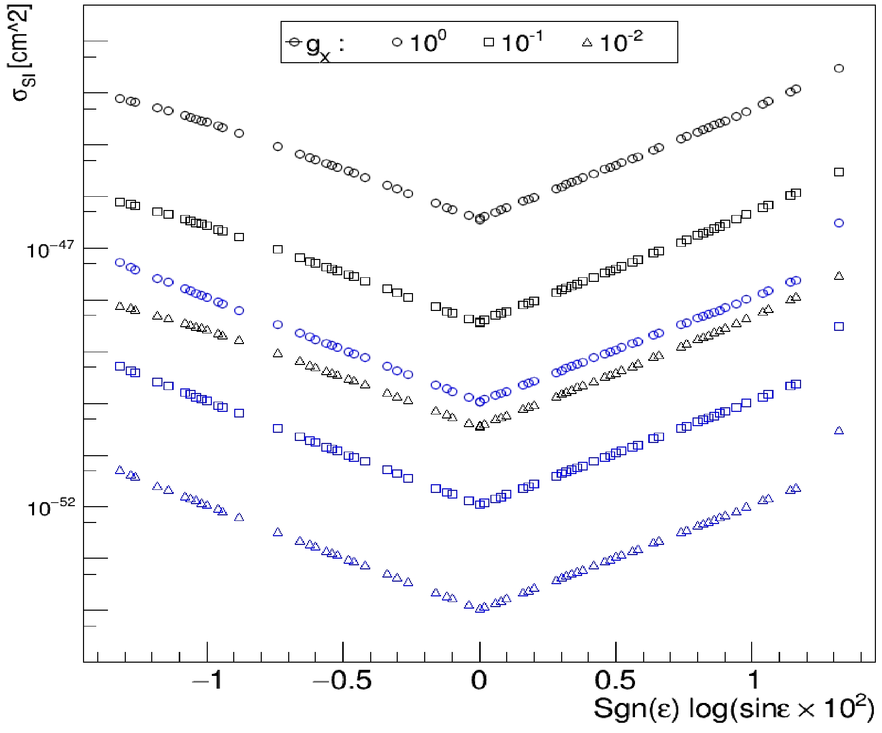

Figure 1.  (color online) $\sigma^{\rm{SI}}_{\chi N}$ dependence on $\sin\varepsilon$ for $m_\chi = 120$${\rm{GeV}}$, $m_{Z^\prime}= 500\; {\rm{GeV}}$, and $g_X = 0.01$ (triangles), $0.1$ (squares), and $1$ (circles). The zero on the horizontal coordinate indicates $\sin\varepsilon = {10}^{-2}$, whereas $\pm 1$ indicates $\sin\varepsilon = \pm {10}^{-1}$. The black points correspond to $\zeta=0$. The blue points are derived by adjusting ζ to achieve a cancellation in $\sigma^{\rm{SI}}_{\chi N}$.

The relic abundance of χ and $\bar\chi$ particles are basically determined by their annihilation cross sections at the freeze-out epoch. To investigate the effect of nonzero ζ in comparison to the case with only kinetic mixing, we compute the total $\chi \bar\chi$ annihilation cross section. The possible two-body annihilation channels involve $f\bar{f}$, $W^+W^-$, $hh$, $ss$, $hs$, $Z^{(\prime)}Z^{(\prime)}$, $hZ^{(\prime)}$, and $sZ^{(\prime)}$. All these channels are mediated via s-channel Z and $Z'$ bosons. In the case of $\zeta = 0$, all of these annihilation processes are controlled by a single parameter $t_{\varepsilon}$, such that they are typically suppressed by the observation that ${\sigma^{SI}_{\chi\; N}}$ is very small. Here, we list two interaction vertices with larger contributions to the annihilation,

where

with ${\widetilde g}_0 = e^2 v /(2 {\hat s}^2_W {\hat c}^2_W)$. Note the presence of the extra parameter ζ, which can mitigate the tension between direct detection and relic abundance. This can be confirmed by the relic density plotted with adjusted ζ in Fig. 2.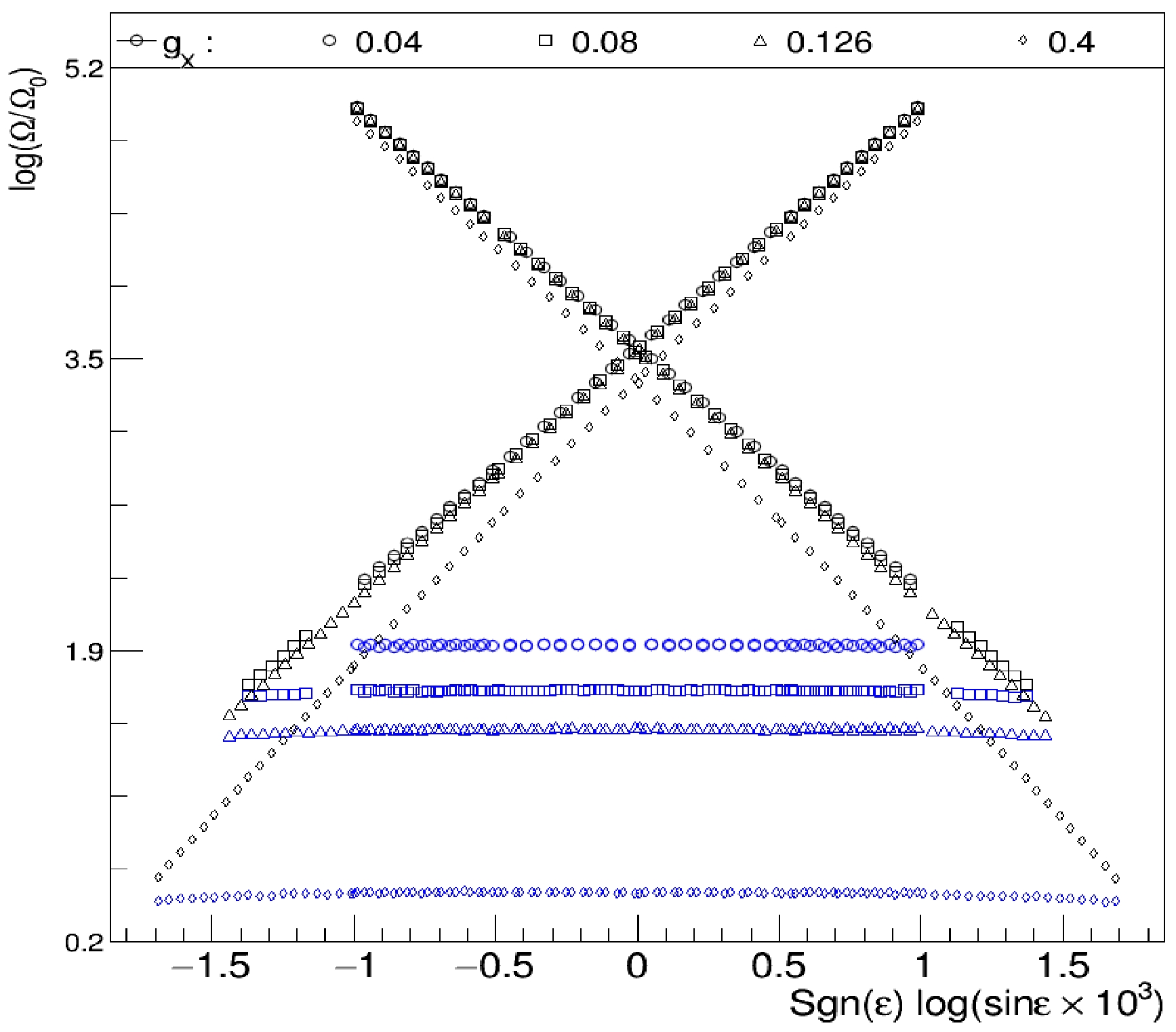

Figure 2.  (color online) DM relic density expressed as $\log(\Omega/\Omega_0)$ for nonzero ζ (blue points) and $\zeta = 0$ (black points) with $m_\chi = 210\; {\rm{GeV}}$, $m_{Z^\prime}= 500\; {\rm{GeV}}$, and $g_X = 0.04$ (circles), $0.08$ (squares), $0.126$ (triangles), and $0.4$ (diamonds). The zero on the vertical coordinate indicates $\Omega=\Omega_0$. The zero on the horizontal coordinate indicates $\sin\varepsilon = {10}^{-3}$, whereas $\pm 1$ indicates $\sin\varepsilon = \pm {10}^{-1}$.

The calculation of the DM relic abundance in our model resorts to numerical procedures, where $\mathrm{micrOmegas}$ [65, 66] is invoked, and Eq. (36) is coded into this framework after double-checks. Attempts to globally explore all the allowed parameter regions are still restrained because the numerical scans fatigue, especially when there are excessive free parameters. To highlight the effect of nonzero ζ, the results in Ref. [26] for $\zeta = 0$ can be taken as a typical reference. To this end, we prepare a scan over the model parameters, where each round of the scan starts from a sampling of parameters $\{g_X, s_\epsilon, s_\xi\}$ running from small to large ⁶. We fix $M_{Z^\prime} = 500\; {\rm{GeV}}$, and $\chi\chi$ annihilation will meet $Z'$ resonance for $m_\chi \sim m_{Z'}/2$.

Given a point in this 3D space, the LEP and LHC constraints mentioned above are calculated first (a failing parameter will be rejected hereafter), and then the effective DM-nucleon cross section is calculated and must satisfy the LZ constraint [63]. Finally, a survival point is fed to the estimation of the relic abundance $\Omega h^2$ and compared with the observed value $\Omega_0 h^2= 0.1200\pm0.0012$ [67].

The scan starts from $m_\chi = (m_h + m_Z)/2 \simeq 115\; {\rm{GeV}}$, but the relic abundance is not satisfied for such low $m_\chi$. Up to $m_\chi = 210\; {\rm{GeV}}$, as shown in Fig. 2, the relic abundance $\Omega h^2$ almost (but not yet, $\log(\Omega/\Omega_0) \sim 0.4$) reaches $0.12$. Nonetheless, such a figure demonstrates that for $g_X = 0.04$, $0.08$, $0.126$, and $0.4$, the obtained relic density for nonzero ζ (blue points) can be decreased by at least two orders of magnitude compared to the black points for $\zeta=0$.

The first physical solution, which passes all the constraints mentioned above and satisfies $|\Omega h^2 - 0.12| \le$ 0.012, is found until $m_\chi = 215\; {\rm{GeV}}$, as shown in Table 2. When the DM candidate become heavier than $260\; {\rm{GeV}}$, which is the last row in this table, physical solutions disappear again. In between, for example, $m_\chi \sim 235\; {\rm{GeV}}$, there are too many solutions to be recorded with $g_X$ running from ${10}^{-1}$ to ${10}^{-3}$. This may simply reflect the the $Z'$ resonance effect (that is, $2 m_chi \simeq m_{Z^\prime}$) [68, 69] for freeze-out DM. In the case of $\zeta = 0$, the resonance region is around $m_\chi \sim 230\text{–}250\; {\rm{GeV}}$, as shown in Fig. 4 of Ref. [26]. The consequence of nonzero ζ is to extend the window to $215\text{–}260\; {\rm{GeV}}$.

$m_\chi$	$g_X$	$s_\varepsilon$	ζ
$215$	$6.31 \times{10}^{-1}$	$5.13 \times{10}^{-2}$	$5.49 \times{10}^{-2}$
$220$	$3.98 \times{10}^{-1}$	$-6.03 \times{10}^{-2}$	$-5.96 \times{10}^{-2}$
$250$	$5.01 \times{10}^{-3}$	$-1.03 \times{10}^{-3}$	$2.70 \times{10}^{-1}$
$260$	$2.512$	$-5.25 \times{10}^{-3}$	$-1.42 \times{10}^{-3}$

Table 2.  Parameters corresponding to the correct relic density and consistent with the constraints. Unshown parameters take values from Ref. [26].

We also rescan around $m_\chi \simeq 115$ GeV but with $m_{Z^\prime}=2.05 m_\chi$ and present a small sample of the solutions in Table 3. The relation $m_{Z^\prime}=2.05 m_\chi$ ensures that the $Z'$ resonance effect is always important at the freeze-out epoch. In the $\zeta = 0$ case, this solution is entirely rejected by the direct detection constraints, as shown in Fig. 5(a) of Ref. [26]. However, in this study, it is recovered with a tuning of ζ.

$g_X$	$s_\varepsilon$	ζ
$1.0 \times{10}^{-1}$	$-1.54\times{10}^{-3}$	$-4.33 \times{10}^{-4}$
$1.0 \times{10}^{-2}$	$-1.83 \times{10}^{-3}$	$-1.03\times{10}^{-1}$
$2.51 \times{10}^{-3}$	$-1.0 \times{10}^{-3}$	$-4.15 \times{10}^{-1}$

Table 3.  Parameters corresponding to the correct relic density and consistent with the constraints for $m_\chi = (m_h +$$m_Z)/2 \simeq 115\; {\rm{GeV}}$ and $m_{Z^\prime}=2.05 m_\chi$.

With $\mathrm{micrOmegas}$, the γ-ray spectrum for DM indirect detection is also investigated to compare it with the upper bounds from Fermi-LAT γ-ray observations [70]. No excess is observed, at least upon the parameters passing the above procedures in Tables 2 and 3.

In this study, we introduce an extra ${{U}}(1)_{{X}}$ gauge symmetry, which is responsible for the interactions of Dirac fermionic DM with a ${{U}}(1)_{{X}}$ charge. In particular, we assume that the SM Higgs doublet also carries a ${{U}}(1)_{{X}}$ charge ζ. To make the SM Yukawa interaction terms gauge-invariant and ensure the theory is free from gauge anomalies, the SM fermions are assigned Y-sequential ${{U}}(1)_{{X}}$ charges proportional to ζ. The mixing between the ${{U}}(1)_{{X}}$ and ${{U}}(1)_{{Y}}$ gauge fields are induced by both kinetic mixing and the ${{U}}(1)_{{X}}$ charge of the SM Higgs doublet. Thus, the DM interactions with SM particles mediated by the Z boson and new $Z'$ boson are essentially controlled by the kinetic mixing parameter $\epsilon$ and Higgs charge ζ.

After the analytical calculation, we perform numerical scans with fixed $m_{Z^\prime}$ over the parameter space of $g_X$, $s_\epsilon$, and ζ. The new parameter ζ is found to invite destructive interference in the effective DM-nucleon cross section and can affect the relic density by approximately two orders of magnitude. Although the magnitude of ζ is small owing to the constraints from LEP and LHC experimental data, the cancellation between the interactions originating from kinetic mixing and Higgs ${{U}}(1)_{{X}}$ charge does take place. Therefore, it can definitely extend the physical windows in which the resonance effect for relic density are important. Nonetheless, the introduction of ζ itself is not sufficient to make generic parameter regions work.

L.Y. SHAN would like to thank Prof. Ying ZHANG for discussions about general U(1)_X from the viewpoint of effective field theory (Stueckelberg mechanism).

By defining $\hat{m}_{Z}^{2} \equiv (\hat{g}^{2}+\hat{g}^{\prime 2})v^{2}/4$, $\hat{m}_{Z^{\prime}}^{2} \equiv g_{X}^{2} (v_{S}^{2} + \zeta^2 v^2)$, the squared masses of the Z and $Z'$ bosons can be expressed as

where the small corrections are recast into

We can easily crosscheck that $C_{Z,Z^\prime}$ approaches $\hat{s}_W t_\epsilon t_\xi$ via Eq. (20) of Ref. [26] in the limit $\zeta\rightarrow 0$. From Eqs. (13), (27), and Eq. (A2), the presence of ζ is observed to result in more tangled nested functions and obstruct a direct elimination of $C_Z$ or ${\hat s}_{\rm{W}}$. Below, an iterative approach is adopted to solve these nested functions.

First, $t_{2\xi}$ can be shaped as a Taylor expansion around $(C_Z,{\hat s}_{\rm{W}}) \simeq (0, s_{\rm{W}})$ :

where $(n+1)$ denotes an approximation after the $n^\text{th}$ iteration. As confirmed below, the contributions from higher orders will be incorporated by balancing the expression with increasing n. The expansion is based on the fact that $C_Z$ is constrained to be small because the Z boson mass $m_Z$ is well-measured, as well as because $\hat{s}_{\rm{W}}$ is known to be close to $s_{\rm{W}}$. More expressions are required to keep the iteration system close:

The leading iteration simply starts from

This is also the leading expression in many previous studies. Together with $\hat{s}^{(1)}_{\rm{W}} = s_{\rm{W}}$, it can be utilized to obtain

When Eqs. (A7) and (A6) are inserted back into Eq. (A3), we can obtain $t^{(3)}_{2\xi}$ in Eq. (28). This expression can be increasingly expanded when the round of iterations is further extended. These formulas are helpful in demonstrating the effects of a nonzero ζ.

Alternatively, because the rotation angle ξ appears more in the Lagrangian, for example, in the interactions among SM particles, especially in the fermion sector, whereas ζ only explicitly appears in the $Z^\prime$ interactions in the Higgs sector, it is convenient to choose ξ as a free parameter and regard ζ as a derived parameter. Therefore, Eqs. (13) and (A2) are helpful in eliminating ζ (and even ${\hat s}_{\rm{W}}$):

In such a choice, we require no more than the renormalization of the Weinberg angle ${\hat \theta}_{\rm{W}}$ via Eq. (27) with a small correction from $C_Z$:

In the case where ζ is explicitly involved, it can be recalculated from

Therein, ${\hat s}_{\rm{W}}$ (${\hat c}_{\rm{W}}$) should be replaced with the above formulation. It is possible that ζ may not be small when r becomes large.

It is also straightforward to iterate $C_{Z^\prime}$ via Eq. (A5), solve

and propagate the basic parameters and corrections to the Higgs sector via

Using the above relations, all the parameters in the model are calculable with $g_X$, $m_{Z^\prime}$, $s_{\epsilon}$, ζ, $m_s$, and $s_{\eta}$, together with the well-measured parameters $G_{\rm{F}}$, $m_Z$, and α.