Nonlinear corrections for the nuclear gluon distribution in eA processes

The dynamics of parton interactions and the partonic structure of nuclei are prime research topics for both particle and nuclear physics. The formation of quark-gluon plasma inside nuclei is explored during the very first fractions of ${\rm{fm}}/c$ in high-energy nuclear collisions. This probe is based on a large momentum (or mass) $Q{\gg}\Lambda_{\rm QCD}$ scale, which is the main motivation for studying nuclear parton distributions. According to the knowledge of the parton distribution functions (PDFs) of free nucleons, arising from the measurements of deeply inelastic scattering (DIS) in lepton-nucleon ($lN$) collisions, the program of extracting nuclear PDFs (nPDFs) also relies on the DIS data [1−3]. The HERA data for the free proton reach $x{\sim}10^{-5}$ for perturbative values of $Q^2$, while the DIS-measurements for nuclear targets are bound to severely higher momentum fractions, $x{\gtrsim}10^{-2}$.

In Ref. [4], the authors studied the prospects for constraining the nuclear parton distribution functions by small-x deep inelastic scattering at the Large Hadron Electron Collider (LHeC) [5], where its extension of the kinematic covers four orders of magnitude in DIS. The effect of high-precision DIS-measurements at the LHeC in Ref. [4] is illustrated by the ratio of the reduced, inclusive DIS cross-sections, $\sigma^{A}_{{\rm{reduced}}}(x,Q^2)/\sigma^{p}_{{\rm{reduced}}}(x,Q^2)$, where

where x, y, and $Q^2$ are the standard DIS variables, and A is the number of nucleons in a nuclear target. The LHeC promises the equivalent of $1\; {\rm{fb}}^{-1}$ of luminosity for ${\rm{ePb}}$ collisions at LH(e)C energies. With its large $Q^2$ and $1/x$ range, nuclear shadowing can be measured very precisely.

At high energies, nuclear shadowing is controlled by coherence effects. Namely, shadowing is possible only if the coherence time exceeds the mean inter-nucleon spacing in nuclei, and shadowing saturates if the coherence time substantially exceeds the nuclear radius [6−8]. Nuclear shadowing at small x (i.e., $x{\lesssim}0.1$) is experimentally well studied by NMC [9]. Experiments at CERN and Fermilab focus especially on the region of small values of the Bjorken variable x and show a systematic reduction of the nuclear structure function $F^{A}_{2}(x,Q^{2})/A$ with respect to the free proton structure function $F^{p}_{2}(x,Q^{2})$. This phenomenon is known as the nuclear shadowing effect and is associated to the modification of the target parton distributions so that $xf_{i}^{A}(x,Q^{2})<Axf_{i}^{p}(x,Q^{2})$, $f_{i}=q,g,..$ [10]. The relation of the bound-proton PDFs with respect to free-proton PDFs $f_{i}^{p}$ is often expressed in terms of the nuclear modification factors $R_{i}^{A}(x,Q^2)=f_{i}^{p/A}(x,Q^2)/ f_{i}^{p}(x,Q^2)$. For a nucleus A with Z protons and $N=A-Z$ neutrons, an average PDF is obtained as

where $f_{i}^{p/A}$ are the PDFs of a bound proton and the neutron contents $f_{i}^{n/A}$ are obtained from $f_{i}^{p/A}$ via isospin symmetry [11−14]. As revealed by DIS experiments, the bound nucleon PDFs are not the same as those of a free proton but are modified in a nontrivial way and obey the Dokshitzer-Gribov-Lipatov-Altarelli-Parisi (DGLAP) evolution [15−18], which describes how the PDFs depend on the factorization scale

with splitting functions $P_{ij}$ governing the scale evolution. For the evolution of the PDFs due to the evolution equation (i.e., Eq. (3)), a non-perturbative input at some initial scale is required to obtain a PDF set. The baseline parton distributions of a proton are parametrized in the following formal form:

where the coefficients $\alpha_{1}$ and $\alpha_{2}$ control the asymptotic behavior of $f_{i}(x,Q^{2}_{0})$ in the limits $x{\rightarrow }0$ and 1, and $P_{i}$ is a sum of Bernstein polynomials dependent on $y=f(x)$, which is very flexible across the whole interval $0<x<1$. For PDFs of nuclei, an additional dependence on the atomic mass A is required [12, 14, 19]. In Ref. [20], the authors discussed the nuclear cross section in terms of nuclear volume and surface contributions

Therefore, the cross section per nucleon is assumed to be proportional to $1/A^{1/3}$ as

If $\sigma_{V}$ and $\sigma_{S}$ depend weakly on A, the $1/A^{1/3}$ dependence makes sense as the leading approximation.

A much harder task has been to determine the gluon distribution of nucleons bound in a nucleus, i.e., the nuclear gluon distribution ($xg^{A}(x,Q^{2})$). The kinematic extension of the electron - Ion collider (EIC) [21, 22] will allow us to examine the non-linear dynamics at low x. When the gluon density becomes sufficiently large at small x, one needs to consider the effects of gluon recombination (gluon-gluon fusion) leading to nonlinear corrections to the DGLAP evolution equations [23−25]. Indeed, the gluon-gluon recombination processes cause the growth of the gluon density to slow down at smaller values of x and $Q^{2}$ (but still $Q^{2}{\gg}\Lambda^{2}_{\rm QCD}$). In the Gribov-Levin-Ryskin-Mueller-Qiu (GLR-MQ) approach [23, 24], the gluon recombination is addressed by analyzing so-called $"$fan$"$ diagrams, where two gluon ladders merge into a gluon or a quark-antiquark pair. Adding these contributions to the DGLAP equations yields the nonlinear GLR-MQ evolution equations [23, 24], where the nonlinear term tames the growth of the PDFs at small x and leads to their suppression. One of the important outcomes of the study in Ref. [26] is the existence of the saturation scale $Q_{s}(x)$ ($Q_{s}^{2}=Q_{0}^{2}(x/x_{0})^{-\lambda}$ where $Q_{0}$ and $x_{0}$are free parameters), which is a characteristic scale at which the parton recombination effects become important. The solution to the non-linear equation has the property of the geometric scaling in the regime where $k<Q_{s}(x )$, whereas in the case when $k>Q_{s}(x)$, the solution enters the linear regime, where k is the gluon transverse momenta.

Effects of small-x nonlinear corrections to the DGLAP evolution equations due to gluon recombination have been extensively studied in the literature [27−32]. Recently, in Ref. [33], the authors considered the nonlinear GLR-MQ evolution equations for nPDFs using the "brute force" method in the momentum space. The authors [33] confirmed the importance of the nonlinear corrections for small $x{\lesssim}10^{-3}$, whose magnitude increases with a decrease in x and an increase in the atomic number A. This paper is organized as follows. In the next section, the theoretical formalism is presented, including the GLR-MQ evolution equation. In Sec. III, we present a detailed analytical analysis and our main results for the nuclear gluon density and predictions of the non-linear effects at higher order accuracy. In the last section, we summarize our findings.

The nonlinear corrections in the GLR-MQ evolution equations for nPDFs are defined by the following forms: ¹

and

where $\dfrac{\partial{f_{i}(x, Q^{2})}}{\partial{\ln}Q^{2}}\Big|_{{\rm{DGLAP}}}$ for the parton distributions refer to the standard DGLAP evolution equations. Here, ${\cal{R}}$ is the characteristic radius of the gluon distribution in the hadronic target. ${\cal{R}}^{A}$ for a nuclear target with the mass number A is defined by ${\cal{R}}^{A}=2\; {\rm{GeV^{-1}}}{\times}A^{1/3}$ [33]. The value of $2\; {\rm{GeV^{-1}}}$ depends on how the gluons have a hotspot-like structure within the nucleon. Here, $\chi=\dfrac{x}{x_{0}}$ and $x_{0}$ is the boundary condition under which the gluon distribution joints smoothly onto the linear region. The second terms in the right-hand sides of Eqs. (7) and (8) are expected to become important and related to the recombination of the gluons in the low-x region, when the gluon density is very large. This is known as the phenomenon of gluon saturation.

Since the parton distributions in bound and free protons are different, $f^{A}(x, Q^2){\neq}f(x, Q^2)$; therefore, the ratio of structure functions is observed to deviate clearly from unity. The nuclear modifications at $x{\lesssim}0.1$ are referred to as shadowing. The nuclear structure function $F_{2}^{A}$ in the QCD-improved parton model (in leading order (LO) of $\alpha_{s}$ or in the DIS-scheme in any higher order) can be written in terms of its parton distributions as

where $e_{q}$ is the quark charge, and $q^{A}(\overline{q}^{A})$ is the quark (antiquark) density in the nucleus A. The nuclear structure function, with assumed flavor symmetric antiquark distributions, becomes a summation of valence quark and antiquark distributions

The nonlinear equations (i.e., Eqs. (7) and (8)) show that the strong rise corresponding to the linear QCD evolution equation at small-x and $Q^2$ can be tamed by screening effects. After the successive integrating of both sides of Eqs. (7) and (8) with respect to $\ln{Q^2}$and some rearranging, we obtain the nonlinear distribution functions in terms of the linear by the following forms:

and

Integrating the first terms in the left and right hands of Eqs. (11) and (12) and using the linear and nonlinear initial conditions $xf^{A}_{i}(x, Q_{0}^{2})$(given by Eqs. (15), (19), and (20) below), we find the nonlinear corrections (NLCs) to the parton distribution functions by the following forms:

and

Here, $xf_{i}^{A}(x, Q^2)$ and $xf_{i}^{A}(x, Q_{0}^2)$ are the linear parton distribution functions at scales of $Q^2$ and $Q_{0}^{2}$, respectively, and obtained from the coupled DGLAP evolution equations using the modified nuclear distribution functions at the initial scale ². The initial nuclear parton distributions are provided at a fixed $Q^{2}$ (${\equiv}Q_{0}^{2}$) due to a free nucleon distribution function $f_{i}(x, Q_{0}^{2})$ and a multiplicative nuclear modification factor, $w_{i}(x, A, Z)$, given as

The nuclear modification is based on the QCD analysis available in the literature [14, 19, 34−38], and assumes the following modification function:

where $H_{i}(x)=b_{i}(A)x+c_{i}(A)x^2 +d_{i}(A)x^3$ is in the cubic form. An advantage of the cubic form with the additional term $d_{i}$ in contrast to a quadratic-type function, i.e., without $d_{i}$, is that the weight function becomes flexible enough to accommodate both shadowing and anti-shadowing in the valence quark distributions [14].

The nonlinear corrections enter both the gluon and the sea-quark distributions at small x through (i) modifications of the initial distributions and (ii) the presence of additional nonlinear terms in the $Q^2$-evolution equations. To study the possible importance of nonlinear corrections, we base our initial gluon and singlet distribution $xg^{\rm NLC}(x, Q_{0}^{2})$ and $xq_{s}^{\rm NLC}(x, Q_{0}^{2})$ by imposing nonlinear corrections on linear distribution functions. The nonlinear corrections to the gluon distribution at the initial scale $Q_{0}^2$ is obtained from the results in Ref. [39] as ³

where

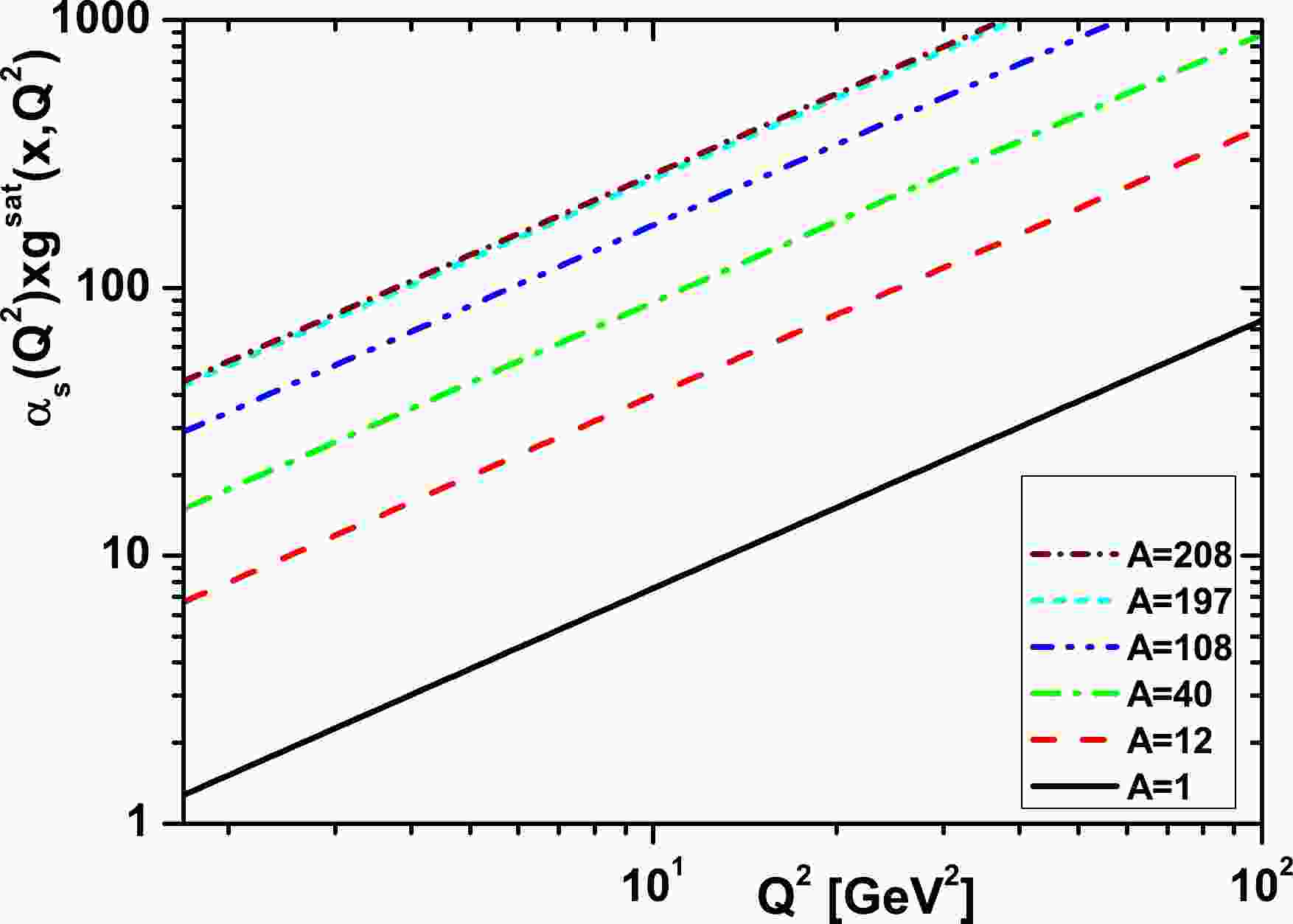
The nonlinear terms in the right-hand side of evolution equations (i.e., Eqs. (7) and (8)) are defined by $xg^{A}_{{\rm{sat}}}$, and this is the value of the gluon which would saturate the unitarity limit in the leading shadowing approximation. In Fig. 1, we show that the gluon saturation as a function of the mass number A is expected to occur for various values of $Q^2$ [40]. In Fig. 2, the gluon distribution, $\alpha_{s}xg^{A}_{{\rm{sat}}}$, increases as the mass number A increases at the initial scale $Q_{0}^{2}=1.69\; {\rm{GeV}}^2$ [41]. Therefore, the effect of the gluon saturation is expected to be larger in heavy nuclei and important for small values of $Q^2$.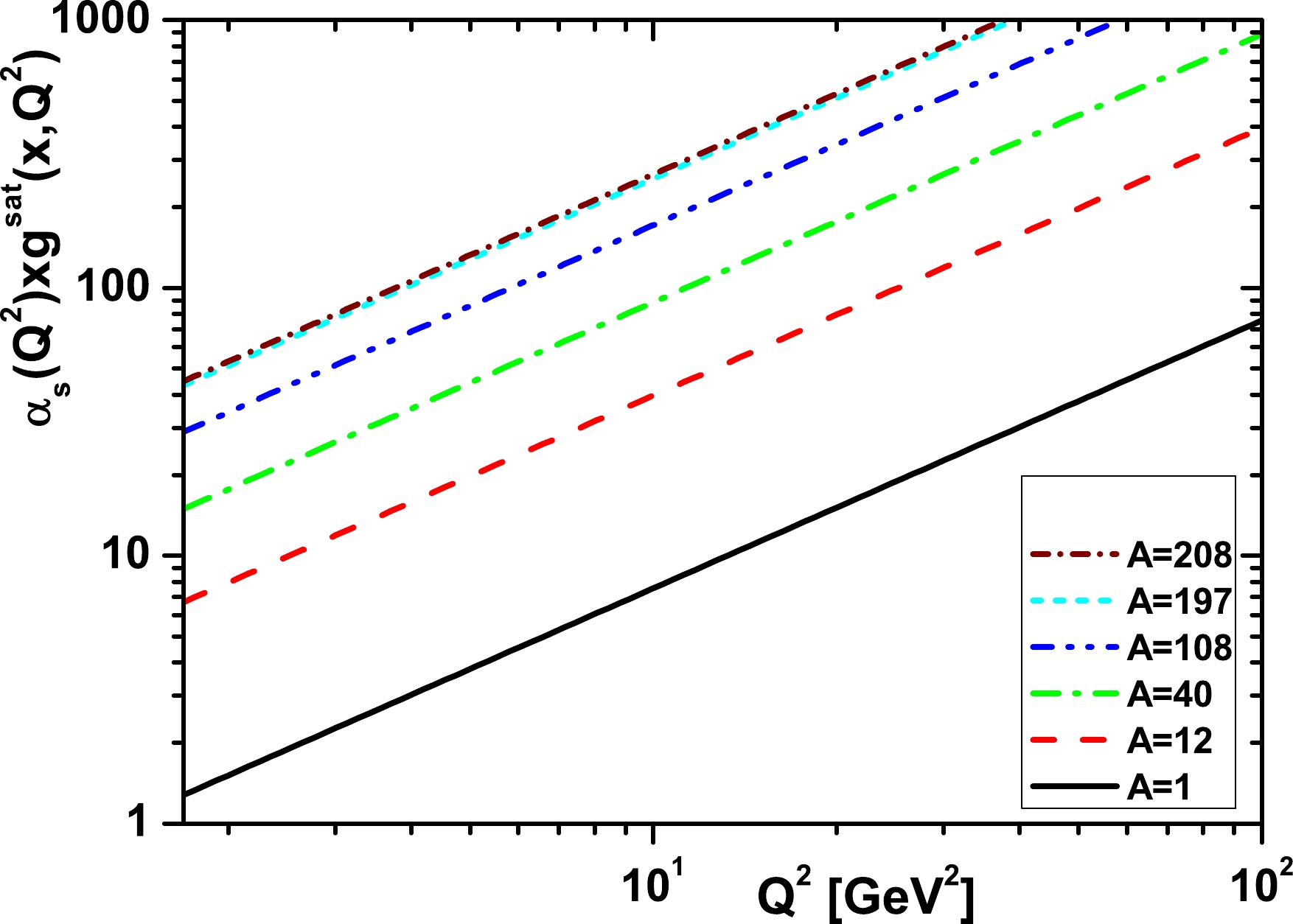

Figure 1.  (color online) Results of $\alpha_{s}xg^{A}_{{\rm{sat}}}$ for different values of $Q^2$ in a wide range of nuclei, including C-12, Ca-40, Ag-108, Au-197, Pb-208, and the free proton.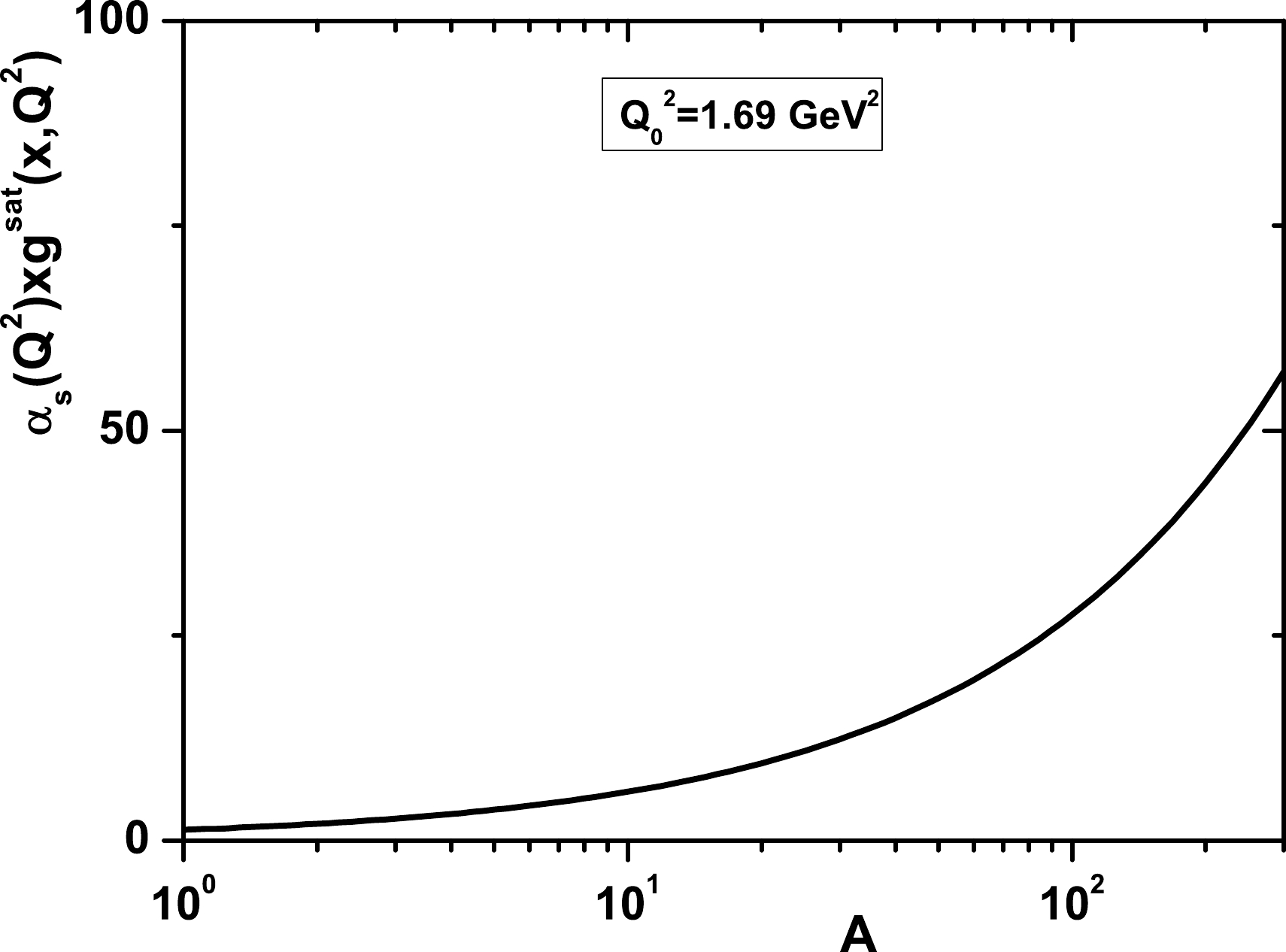

Figure 2.  (color online) Results of $\alpha_{s}xg^{A}_{{\rm{sat}}}$ in a wide range of nuclei at $Q_{0}^2=1.69\; {\rm{GeV}}^2$.

We rewrite Eq. (17) by using Eq. (16) to take into account the nonlinear correction to the nuclear gluon distribution at the initial scale for $x<x_{0}$, given as

We note that in Eq. (19), $xg^{A, {\rm{NLC}}}{\rightarrow }xg^{A}$ when ${\cal{R}}^{A}{\rightarrow }\infty$ and $xg^{A}_{{\rm{sat}}}{\rightarrow }\infty$. Also, we see that $xg^{A, {\rm{NLC}}}{\rightarrow }xg^{A}_{{\rm{sat}}}$ when $x{\rightarrow }0$. Moreover, $xg^{A, {\rm{NLC}}}$ joins smoothly onto $xg^{A}$ at $x=x_{0}(=10^{-2})$. The nonlinear corrections to the gluon distribution are reflected in the sea-quark distributions $q^{A}_{s}(x, Q^{2})$, which, at small x, are predominantly driven by the gluon and modify the nuclear structure function as ⁴

The weight function $w_{i}(x, A, Z)$ for the linear distribution functions can be obtained from the three constrains for the nuclear distributions as the nuclear charge Z, mass number A, and momentum conservations ⁵ are defined by the following forms [14, 19, 33−38]:

For a detailed investigation of these functions, we constrain our results to the functions defined in Ref. [35]. The gluon distribution at low x is dominant. Therefore, we used the standard gluon distribution at the input scale $Q_{0}^{2}=1.69\; {\rm{GeV}}^2$ obtained from the CT18 set of the free proton PDFs [43], i.e.,

where the coefficients $a_{0-4}$ are listed in Ref. [43]. The weight function $w_{g}(x, A, Z)$ for the gluon distribution function is defined by the following form [35]:

where the coefficients at the next-to-leading order (NLO) and the next-to-next-to-leading order (NNLO) approximations are listed in Ref. [35]. The strong coupling is set equal to $\alpha_{s}(M_{z})=0.118$ for both the NLO and NNLO approximations. In Figs. 3 and 4, we show representations of the nonlinear corrections to the gluon modification functions at the initial scale $Q_{0}^{2}=1.69\; {\rm{GeV}}^{2}$ for two selected nuclei, C-12 and Pb-208, at the NLO and NNLO approximations, respectively. The nuclear gluon distribution functions are analyzed using the CT18 proton PDF set as a baseline in these figures (i.e., Figs. 3 and 4) [43]. The nuclear modification factors are extracted from QCD fits to the nuclear and neutrino(antineutrino) DIS and Drell-Yan data ⁶. The resulting nonlinear corrections to the gluon distribution function are presented in Fig. 5 for carbon (left) and iron (right) at $Q_{0}^{2}=2\; {\rm{GeV}}^{2}$ in the NLO approximation. To achieve this, we used the gluon distribution for a free proton defined in Ref. [44] as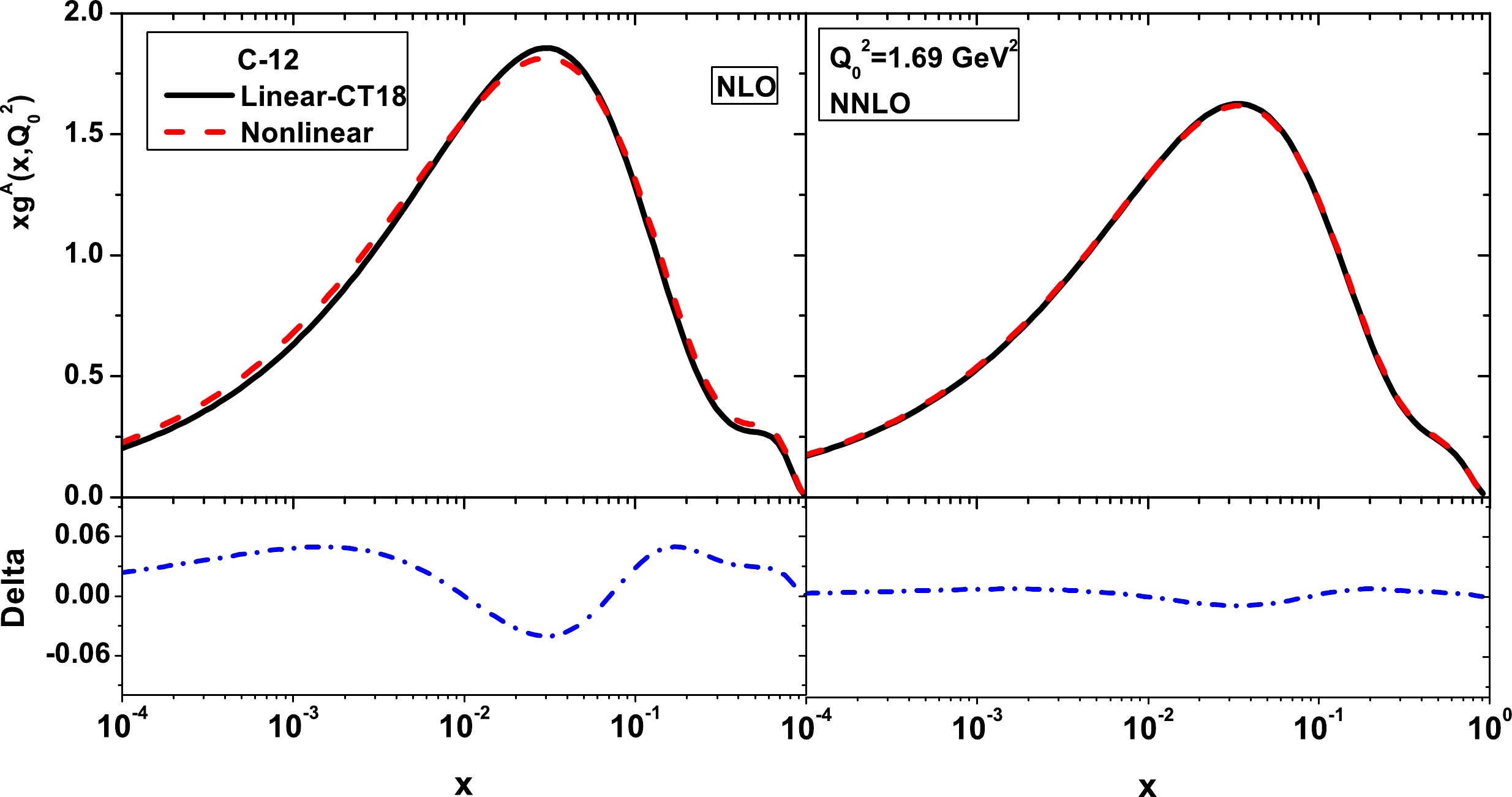

Figure 3.  (color online) Nonlinear gluon distribution function ($xg^{A, {\rm{NLC}}}(x, Q_{0}^{2})$) compared with the linear ($xg^{A}(x, Q_{0}^{2})$) for C-12 at $Q_{0}^2=1.69\; {\rm{GeV}}^2$ in the NLO and NNLO approximations. The delta values are differences between the nonlinear and linear distribution functions (${\rm{Delta}}=xg^{A,\rm NLC}(x, Q_{0}^{2})-xg^{A}(x, Q_{0}^{2})$) at the initial scale.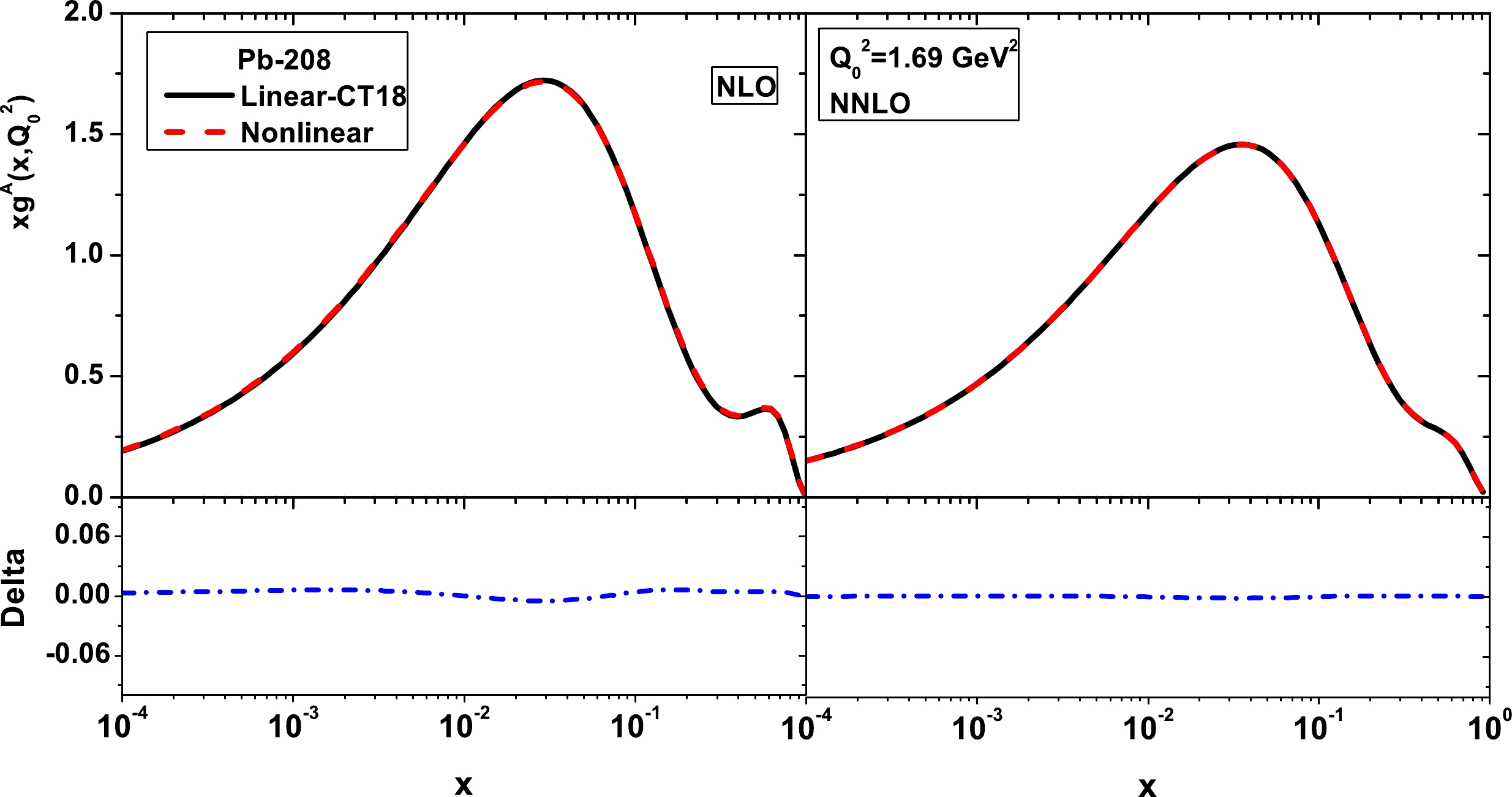

Figure 4.  (color online) Same as Fig. 3 but for lead.

Figure 5.  (color online) Nonlinear gluon distribution function ($xg^{A, {\rm{NLC}}}(x, Q_{0}^{2})$) compared with the linear ($xg^{A}(x, Q_{0}^{2})$) for carbon (left) and iron (right) at $Q_{0}^2=2\; {\rm{GeV}}^2$ in the NLO approximation. The delta values are differences between the nonlinear and linear distribution functions (${\rm{Delta}}=xg^{A,\rm NLC}(x, Q_{0}^{2})-xg^{A}(x, Q_{0}^{2})$) at the initial scale.

where the coefficients at the NLO approximation are listed in Refs. [19, 44]. The weight function for the nuclei of carbon and iron has the same form in Eq. (16), and the coefficients are presented in Ref. [19] in which the effects of shadowing, anti-shadowing, fermi motion, and the EMC regions are included.

In Fig. 6, we compare the nonlinear and linear gluon distributions in lead at the NNLO approximation to those of JR09 [45] at $Q_{0}^{2}=2\; {\rm{GeV}}^2$. The nuclear gluon distribution is obtained from JR09 parametrization at the input scale by the following form of the free proton PDFs:

Figure 6.  (color online) Nonlinear gluon distribution function ($xg^{A, {\rm{NLC}}}(x, Q_{0}^{2})$) compared with the linear ($xg^{A}(x, Q_{0}^{2})$) for lead at $Q_{0}^2=2\; {\rm{GeV}}^2$ in the NNLO approximation. The delta values are differences between the nonlinear and linear distribution functions (${\rm{Delta}}=xg^{A,\rm NLC}(x, Q_{0}^{2})-xg^{A}(x, Q_{0}^{2})$) at the initial scale.

where the parameters in the weight function are in Ref. [34]. To quantify the magnitude of NNLO corrections, we present the nonlinear corrections of nuclear gluon distributions obtained at the input scale of the CT18 and JR09 parametrizations in Figs. 3, 4, and 6 for light and heavy nuclei. The Delta functions in these figures show that the nonlinear and linear gluon distributions have a similar behavior at the input scale in a wide range of x. Therefore, Eq. (13) changes to an approximate relation at the NNLO accuracy as

In Figs. 3−5, we observe that $xg^{A, {\rm NLC}}(x, Q_{0}^{2}){\neq}xg^{A}(x, Q_{0}^{2})$ at the NLO accuracy. Therefore, the evolution of the nuclear gluon distribution functions with the nonlinear corrections are defined by the following form:

For the evolution of the nonlinear corrections of the nuclear gluon distributions, we need to a gluon analytical distribution function for a free proton at the $Q^2$ scale in the NLO and NNLO approximations. Usually, the gluon analytical distribution function at the LO approximation is defined in previous studies. To do it, we extend the analytical solution used in the DGLAP evolution to consider the nonlinear corrections in Eqs. (27) and (26) at the NLO and NNLO approximations, respectively. In the next section, we solve the DGLAP evolution equation using Laplace transform techniques.

According to the DGLAP $Q^{2}$-evolution equations, the singlet distribution function leads to the following integro-differential equation:

where $P_{qq}$ and $P_{qg}$ are the quark-quark and quark-gluon splitting functions calculated to the desired order in $\alpha_{s}$ [46−48]. Here, $<e^{2}>$ is the average of the charge $e^{2}$ for the active quark flavors. Also, $<e^{2}>=n_{f}^{-1}\sum_{i=1}^{n_{f}}e_{i}^{2}$, and the symbol $\otimes$ denotes convolution according to the usual prescription. Considering the variable definitions $\upsilon{\equiv}\ln(1/x)$ and $w{\equiv}\ln(1/z)$, one can rewrite Eq. (28) in terms of the convolution integrals and new variables as

where

The Laplace transform of ${\cal{\widehat{H}}}(\alpha_{s}(Q^{2}), \upsilon)$, are given by the following forms:

Consequently, we can rewrite Eq. (29) in the Laplace space s by using the convolution theorem for Laplace transforms and considering the fact that the Laplace transform of the convolution factors is simply the ordinary product of the Laplace transform of the factors, i.e.,

where

and

The coefficient functions Φ and Θ in the Laplace space s at the LO approximation are given by

where $\psi(x)$ is the digamma function and $\gamma_{E}=0.5772156 . . .$ is the Euler constant.

The explicit expressions for the NLO and NNLO kernels in s space are rather cumbersome; therefore, we recall that we are interested in investigating the kernels in small x [49−51]. In the Laplace space, we consider the kernels at small s, with the two and three-loop kernels given as

and

with the color factors $C_{A}=N_{c}=3$, $C_{F}=\dfrac{N_{c}^{2}-1}{2N_{c}}=\dfrac{4}{3}$, and $T_{f}=\dfrac{1}{2}n_{f}$, associated with the color group $S U(3)$, where $n_{f}$ represents the number of flavors.

Strong coupling satisfies the renormalization group equation, which, up to the NNLO, reads

where $\beta_{0}$, $\beta_{1}$, and $\beta_{2}$ are the one, two, and three loop corrections to the QCD β-function. The standard representation for QCD couplings in the NLO and NNLO (within the ${\rm{\overline{MS}}}$-scheme) approximations have the forms

where $t=\ln\dfrac{Q^{2}}{\Lambda^{2}}$, and Λ is the QCD cut-off parameter [52].

Consequently, the discretized form of Eq. (32) for the gluon distribution reads

where the kernels $k^{(\varphi)}(\alpha_{s}(Q^{2}), s)$ and $h^{(\varphi)}(\alpha_{s}(Q^{2}), s)$ contain contributions of the s-space splitting and coefficient functions up to the NNLO approximation. These kernels can be evaluated from s-space results in the following forms:

The inverse Laplace transform of coefficients $k(a_{s}(Q^{2}), s)$ and $h(a_{s}(Q^{2}), s)$ in the above equations are defined respectively as kernels

and

The kernels are dependent on υ and the running coupling at the higher order approximations. In order to obtain an analytical form for these kernels at higher order approximations, we consider the terms on the order of $1/s$, as these terms are dominant at higher orders [53]. Therefore, we have

Consequently, the general analytical expressions for the gluon distribution function in x-space at the higher order approximations are given by

Having an analytical proton structure function and its derivative with respect to $\ln{Q^{2}}$, one can extract the gluon distribution function at any desired x and $Q^{2}$ values.

Using a parametrization suggested by the authors in Ref. [54] on the proton structure functions in full accordance with the Froissart predictions [55]. The explicit expression for the $F_{2}$parametrization, obtained from a combined fit of the H1 and ZEUS collaboration data [56] in the range of the kinematical variables x and $Q^{2}$($x<0.01$ and $0.15< Q^{2}<3000\; {\rm{GeV}} ^{2}$), is given by

and

where

Here, M and $\mu^{2}$ are the effective mass and scale factor, respectively. The effective parameters in Eq. (44) are defined in Refs. [54] and [57].

Using the analytical approach outlined above (i.e., Eq. (42)) in the NLO and NNLO approximations, we solve the nonlinear gluon distributions for nuclei at low x as

and

Now, we present our numerical results of the nonlinear gluon distribution for light and heavy nuclei in the $x-Q^2$ kinematic regions, where the nonlinear corrections are important. The computed results of the nonlinear gluon distribution function for Au-197 compare with the suggested method by Rausch, Guzey, and Klasen (the RGK model) [33]. This was based on the brute force method, where the authors in Ref. [33] extended the numerical algorithm used in the ${\rm{QCDNUM16}}$ DGLAP evolution code [58] to consider the nonlinear corrections, as the nCTEQ15 nPDFs [59] are used as baseline PDFs.

In Fig. 7, we show representations of the nonlinear gluon distribution functions for Au-197 at scales $Q^2=4, \; 16$, and $100\; {\rm{GeV}}^2$ as a function of the momentum fraction x to show the effects of the $Q^2$ evolution. The nuclear weight functions for the gluon are extracted from the suggested method by Khanpour, Soleymaninia, Atashbar Tehrani, Spiesberger, and Guzey (the KSASG20 model) [35], where the CT18 nPDFs [43] are used as baseline PDFs. These results are compared to the RGK model [33], where the nCTEQ15 nPDFs [59] are used as baseline PDFs in the nonlinear GLR-MQ evolution equation. In the RGK model, the dashed-dot curves show the results of the upward evolution from $Q_{0}^{2}=4\; {\rm{GeV}}^2$ to $Q^2=16$ and $100\; {\rm{GeV}}^2$ (green curves). They also show the results of the downward evolution from $Q_{0}^{2}=100\; {\rm{GeV}}^2$ to $Q^2=16$ and $4\; {\rm{GeV}}^2$ (purple curves) [33]. The uncertainties, due to the statistical errors of the coefficient functions of the parametrization of the proton structure function [54] and the nuclear modification functions [35], are shown in Fig. 7. For the NLO analysis, the nonlinear nuclear distribution function for the gluon shows an increase as x decreases, which is similar to what one can observe in the analyses by RGK [33]. However, the magnitude of these results slightly differs at different scales, but they are within the uncertainty error bands. As can be seen in the figure, the nonlinear gluon densities come with relatively large error bands at the critical point between the linear and nonlinear (i.e., $x=0.01$), reflecting the fact that there are large errors due to the coefficients in the parametrization of the proton structure function.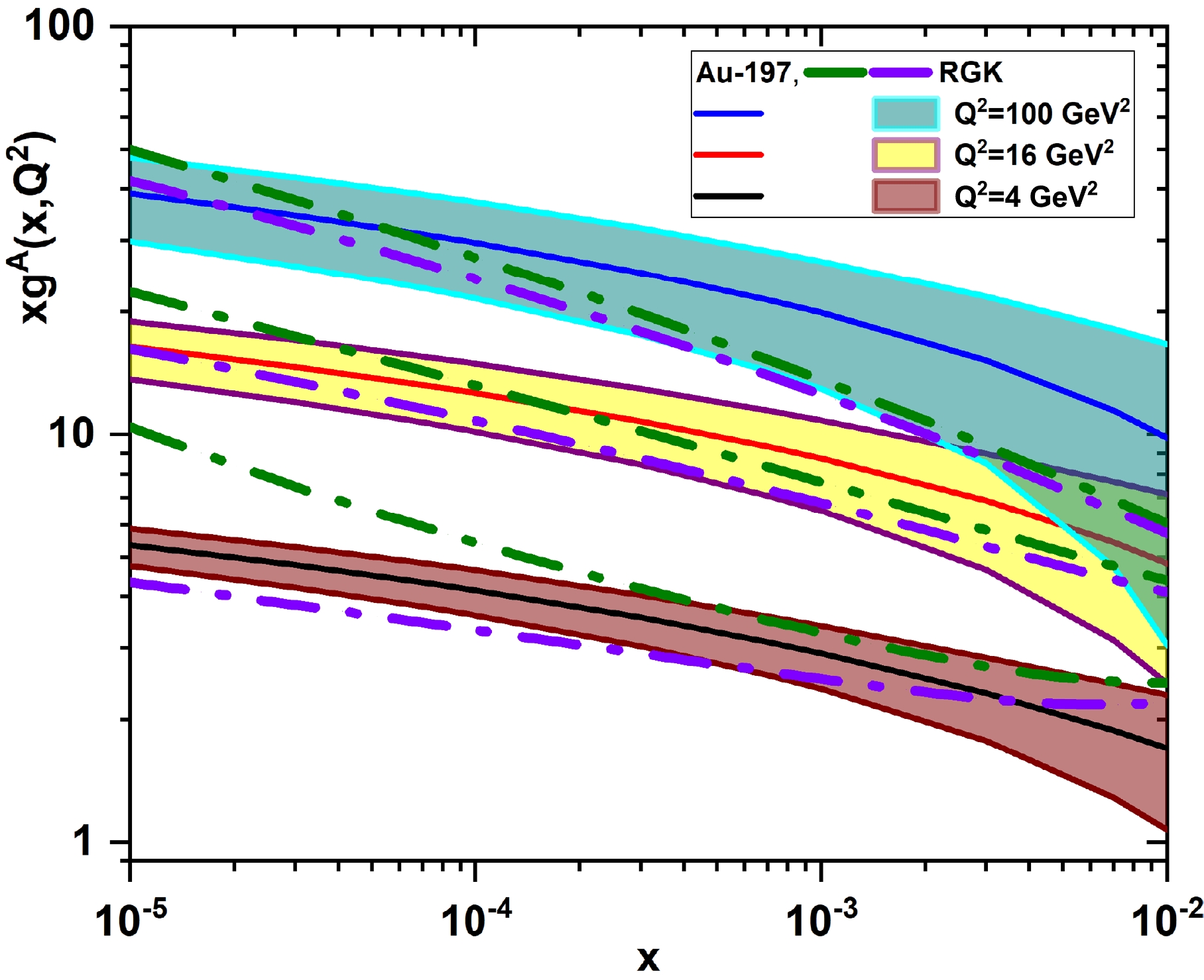

Figure 7.  (color online) Nonlinear gluon distribution functions ($xg^{A, {\rm{NLC}}}(x, Q^{2})$) and their uncertainties at $Q^2=4, \; 16$, and $100\; {\rm{GeV}}^2$ for Au-197 compared with the results of the nonlinear GLR-MQ gluon distribution function (the RGK model) [33]. The dashed-dot lines (green and purple curves) are upward and downward evolutions [33].

In Fig. 8, the nonlinear gluon distributions for C-12 and Pb-208 at the NLO approximation are considered at $Q^2=4$ and $100\; {\rm{GeV}}^2$ as a function of x and accompanied by their uncertainties. To quantify the magnitude of the nonlinear corrections, we present ratios of nuclear gluon distributions obtained in the nonlinear corrections over those of the linear. Figure 9 quantifies the size of the nonlinear corrections as a function of the mass numbers A and x for C-12 and Au-197 at $Q^2=4$ and $100\; {\rm{GeV}}^2$. The difference between the nonlinear and linear evolved gluon densities grows steadily with a decrease of x. This is largest at the smallest values of x and $Q^2$ and disappears for $x=0.01$. The saturation gluon increases as the atomic number increases. Therefore, the nonlinear/linear ratio decreases as the atomic number increases. As one can see, the nonlinear/linear ratio is slightly larger for light nuclei than for heavy nuclei. As expected, this effect is mainly due to the large gluon saturation values of heavy nuclei.

Figure 8.  (color online) Nonlinear gluon distribution functions ($xg^{A, {\rm{NLC}}}(x, Q^{2})$) and their uncertainties at $Q^2=4$ and $100\; {\rm{GeV}}^2$ for C-12(left) and Pb-208(right) as a function of x.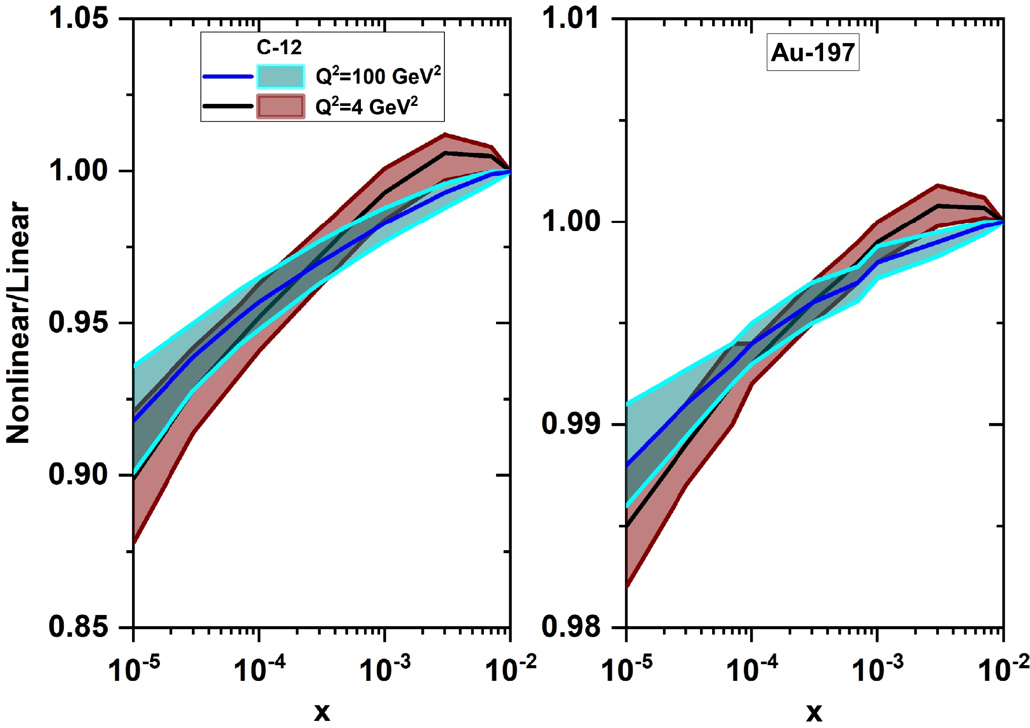

Figure 9.  (color online) Ratio of nonlinear/linear gluon distributions for C-12 and Au-197 at $Q^2=4$ and $100\; {\rm{GeV}}^2$ as a function of x with their uncertainties.

In Figs. 10 and 11, the nonlinear corrections to the gluon distribution function at the NLO approximation for the C-12 and Pb-208 nuclei are presented at $Q^2=10$ and $100\; {\rm{GeV}}^2$ as a function of the momentum fraction x, respectively. In these figures, our numerical results, which are accompanied by statistical errors, are compared with the linear results based on the KSASG20 (NLO) parametrization [35]. The KSASG20 parametrization is a new set of nuclear parton distribution functions (nuclear PDFs) at the NLO and NNLO approximations in perturbative QCD, which include the new CT18 PDFs on proton PDFs. These figures show the effects of nonlinear corrections are noticeable at small x values, and the strong growth of the gluon distributions is tamed by shadowing effects as x decreases. The solid curves represent the effect of shadowing correction for ${\cal{R}}^{A}=2A^{1/3}\; {\rm{GeV}}^{-1}$obtained using Eq. (45). As can be observed, the nuclear gluon distributions increase as x decreases, corresponding to the perturbative QCD fits at small x. However, these behaviors are tamed with respect to the nonlinear terms in the GLR-MQ equation. These tamed behaviors of nuclear gluon distributions due to the shadowing corrections satisfy the Froissart bound in the perturbative QCD mean. Hence, as one can see from Figs. 10 and 11, the deviations from the linear nuclear gluon distributions based on the KSASG20 (NLO) parametrization increase as x decreases. The deviations from the KSASG20 (NLO) nPDFs increase as $Q^2$increases, and they decrease as atomic number A increases (indeed, the nonlinear nuclear gluon distributions increase as atomic number A increases). Significant effects are found for heavier nuclei, such as lead. These behaviors for the nonlinear nuclear gluon distributions are similar to those from the analysis of RGK [33].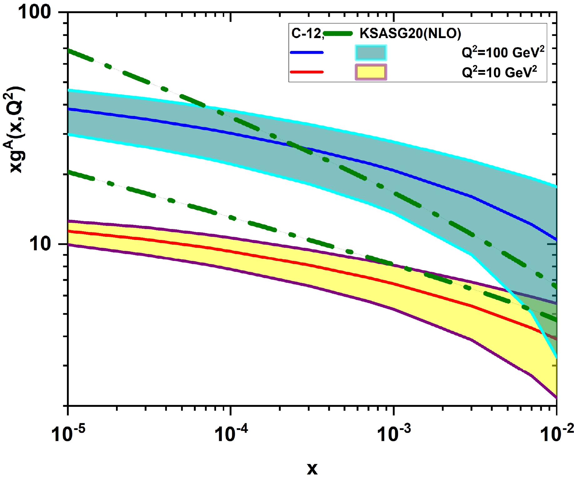

Figure 10.  (color online) Nonlinear gluon distribution functions ($xg^{A, {\rm{NLC}}}(x, Q^{2})$) and their uncertainties at $Q^2=10$ and $100\; {\rm{GeV}}^2$ for C-12 compared with the linear results based on the KSASG20 (NLO) model (dashed-dot curves) [35].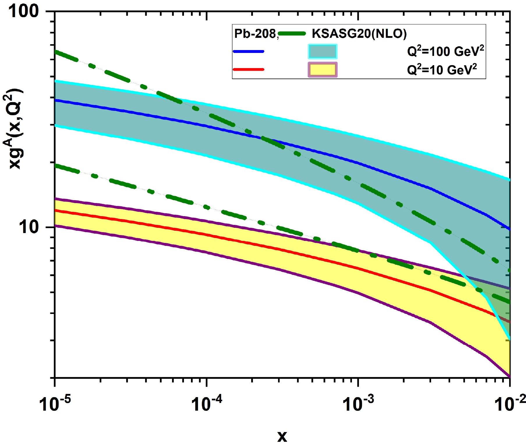

Figure 11.  (color online) Same as Fig. 10 but for Pb-208.

We conducted an analytical study on the effects of adding the nonlinear corrections to the gluon distribution function for light and heavy nuclei at small x. We used the parametrization of the proton structure function to consider an analytical solution for the gluon density at low x in the NLO approximation. The nuclear modification factors are obtained from KSASG20 nuclear PDFS, which are based on the CT18 framework. The shadowing effects of the gluon distribution at small x through modifications of the starting distributions and the presence of additional nonlinear terms in the initial point $Q_{0}^{2}$ at the NLO and NNLO approximations for light and heavy nuclei were considered. We obtained the nonlinear corrections for small x in a wide range of $Q^2$ values. These results show that the magnitude of the nonlinear corrections increases with a decrease in x and an increase in the atomic number A. Our results are consistent, within uncertainties, with the determination of nuclear gluon distribution using the upward and downward evolution from the RGK model, with nCTEQ15 nPDFs as the input. Our determination of nuclear gluon distributions includes error estimates obtained with respect to the coefficient errors in the parametrization of the proton structure function and the nuclear modification function errors. We found differences between our results and those of the RGK model in terms of the NLO accuracy; these differences occur based on the difference in assumptions, such as the input parametrizations and the approximate relation between the gluon distribution and the proton structure function due to the Laplace transform method at low x. These results for the nonlinear corrections to the nuclear gluon distribution function may be important for future experiments at the Electron-Ion Collider [21, 22], LHeC Collaboration, Future Circular Collider (FCC) [5], and Electron-Ion Collider in China (EiCC) [60] at low x.

We are grateful to Razi University for financially supporting this project. G.R. Boroun thanks V. Guzey for allowing access to data related to the nonlinear corrections for the gluon distribution function for Au-197.

Previous studies of the GLR-MQ terms in the context of extracting the parton distribution functions can be found in Ref. [39]. The nonlinear evolution equations relevant at high gluon densities have been studied at small x, where we expect annihilation or recombination of gluons to occur. A measurement of $g(x, Q^2)$ in this region probes a gluon of transverse size $\sim 1/Q$. Therefore, the transverse area of the thin disc they occupy is $\sim xg(x, Q^2)/Q^2$. The shadowing effects, at sufficiently small x where $W{\lesssim}\alpha_{s}$, can be calculated in perturbative QCD. Here, $W{\sim}\dfrac{\alpha_{s}(Q^2)}{\pi{{\cal{R}}^2}Q^2}xg(x, Q^2)$, where $\pi{{\cal{R}}^2}$ is the transverse area and ${\cal{R}}$ is the proton radius. The QCD evolution equation modified for the gluon distribution is defined by the following form:

where the θ function reflects the ordering in longitudinal momenta, and as for $x{\geq}x_{0}$, the shadowing correction is negligible ($x_{0}{=}10^{-2}$). The shadowing term has a minus sign because the scattering amplitude corresponding to the gluon ladder is predominantly imaginary. Equation (47) can be rewritten with a variable change ($x'=\dfrac{x}{z}$) as

There are also shadowing corrections to the evolution equation for the sea-quark distributions, given as

where the higher dimensional gluon term ${\rm{G_{HT}}}$ here is assumed to be zero.

The standard DGLAP evolution equation for singlet and gluon distributions has the following forms:

where $P_{ij}^{, }$s are the splitting functions in the desired order in $\alpha_{s}$.