


 Abstract
 HTML
HTML Reference
 Related
 PDF
PDF


-
The inflationary paradigm has emerged as an elegant solution to several challenges within the standard model of cosmology [1, 2] and it has captured the interest of numerous researchers since its proposal. Precise experimental measurements of the cosmic microwave background (CMB) radiation temperature and anisotropic polarization provide strong support for the slow-rolling inflation [3, 4]. Theoretical investigations have led to the proposal of numerous inflation models, with the single-field inflation model being the simplest and most widely studied. Examples of such models include polynomial potential models [5–8], the Starobinsky model [9–11], Higgs inflation [12–16], natural inflation [17–20], and hilltop inflation [21–23].
The testing of numerous inflation models has become a key challenge in the field of inflationary physics. However, direct observations of inflation in the early universe are not possible, and researchers rely on indirect methods to test these models. A common approach utilizes the scalar spectral index and tensor-to-scalar power ratio, which are predicted using Planck's observations of the CMB. As the accuracy of Planck's observations has improved, many polynomial inflation models have been excluded [3, 4]. However, a promising solution to this problem is to consider the non-minimal coupling between the scalar inflaton and Ricci scalar. This framework offers a mitigation scheme that can potentially rescue a significant number of inflation models [24–27]. Incorporating this non-minimal coupling can alleviate the problematic aspects of certain inflation models, providing a more favorable agreement with the observational data from Planck and preserving their viability.
Considerable efforts have been devoted to further constraining scalar inflation models by exploring the interconnectedness of various physical phenomena. After inflation ends, the universe enters a reheating stage [28–32], during which the inflaton decays into standard model particles or even dark matter particles, and the universe is heated. Thus, the reheating may provide a platform to study inflation.
The limitations of reheating in the context of the single-field scalar inflation model have been extensively studied in Ref. [33]. Reheating involves a preheating process during the early stages, as described in works such as [29, 30, 34–37]. The preheating phase is crucial as it enables the efficient transfer of energy from the inflaton field to the coupled fields. This rapid, non-thermal process is vital for reheating the universe, establishing the initial conditions for the hot Big Bang phase. Without preheating, the transition from the inflationary phase to the radiation-dominated era would occur at a considerably lower pace and with lower efficiency, possibly resulting in discrepancies with observational cosmology. The presence of preheating can be discerned through its influence on the power spectrum of CMB fluctuations and the formation of large-scale structures. Specifically, models with preheating predict distinct non-Gaussianities in the CMB fluctuations, which can be probed by current and future observational missions.
A comprehensive analysis of the interplay between preheating and inflation is presented in Ref. [38]. Furthermore, the constraints imposed by preheating on α-attractor inflation models are investigated by allowing for flexible parameter options in the properties of the preheating stage, as discussed in Ref. [39]. The complexity of the preheating process results from several factors, including the non-perturbative generation of material particles and rapid energy transfer. This complexity results in highly nonlinear and uncertain physics, complicating the study of preheating and necessitating careful consideration of its implications on inflationary models.
Many non-perturbative reheating models have been proposed to study the nature of preheating, including the parametric resonance model [30, 40], hyperluminal instability model [41–43], instantaneous preheating model [44–46], and holographic preheating cosmological model [47, 48]. In our study, we investigate the inflation model by leveraging the properties of preheating. Specifically, we consider the minimal scalar inflation model, which is a simplified version derived from the polynomial potentials model. To analyze the preheating stage, we employ the LATTICEEASY simulation framework [49], which enables us to replicate and study the evolution of preheating processes.
Specifically, we extensively investigate the evolution of particle number density, scale factor, and energy density during the preheating process using LATTICEEASY simulations. By analyzing the simulated data, we deduce important parameters such as the energy ratio (γ) and e-folding number of preheating (
$ N_{\rm pre} $ ). Additionally, we establish an analytical relationship between the preheating process and the inflation model under study. By combining this analytical relation with the observed properties of preheating, we derive constraints on the minimal scalar inflation model. These constraints provide valuable insights into the viability and parameter space of the inflation model, thereby enhancing our understanding of its dynamics and predictions.The remainder of this paper is organized as follows. In Sec. II, we briefly review the minimal scalar inflation model and preheating constraints, and we study the S-field driven inflation in detail. In Sec. III, we describe the simulation of the preheating using LATTICEEASY and discuss the evolution of particle number density, scale factor, and energy density. Numerical analysis and discussion are presented in Sec. IV. A summary is given in Sec. V.
-
Because inflation is driven by the S-field, we can express the corresponding action as
$ S_J = \int {\rm d}^4 x \sqrt{-g} \left[\frac{M_P^2}{2} R \left(1 + 2 \xi_S \frac{S^2}{M_P^2} \right) -\frac{1}{2} \left(\partial S \right)^2 - V(S) \right]\,, $

(1) Following the conformal transformation strategy [50], the action
$ S_E $ in the Einstein frame can be easily obtained as$ S_E = \int {\rm d}^4 x \sqrt{- \tilde{g}} \left[\frac{M_P^2}{2} \tilde{R} - \frac{1}{2 } \left(\tilde{\partial} \bar{S} \right)^2 - V(\bar{S}) \right], $

(2) where the potential
$ V(\bar{S}) $ is expressed as$ V (\bar{S})= \frac{\lambda_S M_P^4}{16 \xi_S^2} \left(1 - {\rm e}^{- 2{\sqrt{\frac{2}{3}}} \frac{\bar{S}}{M_P} } \right)^2, $

(3) and the relation between the refined
$ \bar{S} $ -field and S-field is expressed as$ \bar{S}= \sqrt{\frac{3}{8}} M_P \ln \left(1+ \frac{2\xi_S S^2}{M_P^2} \right). $

(4) The variation in potential V with
$ \bar{S} $ , shown in Fig. 1, indicates that the trend of the potential is independent of the coefficient$ \xi_S $ and$ \lambda_S $ . As$ \bar{S} $ increases, V increases, and after some time, it reaches a plateau, which enables a slow-rolling inflation.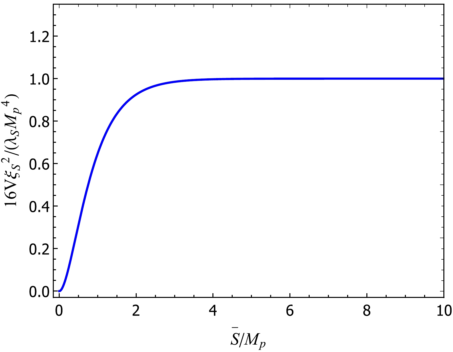
Figure 1. (color online) Variation in the slow-rolling inflationary potential with respect to inflaton, which is calculated using Eq. (3). In the early stages of inflation, the scalar field rolls slowly in the direction that it falls. Subsequently, when the potential energy is no longer dominant, inflation ends.
Given the potential, we can study cosmological inflation in detail. For the e-folding number between the horizon exit of the pivot scale and the end of inflation, it can be analytically calculated according to the following formula [51]:
$ N_k = \frac{1}{M_P^2} \int_{\bar{S}_{\rm end}}^{\bar{S}_k} \frac{V}{V'}\, {\rm d} \bar{S}=\frac{\sqrt{6}}{8 M_P} \left[\frac{\sqrt{6}M_P }{4} {\rm e}^{ 2{\sqrt{\frac{2}{3}}} \frac{\bar{S}}{M_P} } - \bar{S} \right] \Big|^{\bar{S}_k}_{\bar{S}_{\rm end}}. $

(5) Because
$\bar{S}_k \gg \bar{S}_{\rm end}$ , and$\dfrac{\sqrt{6}M_P }{4} {\rm e}^{\sqrt{\frac{2}{3}} \frac{\bar{S}_k}{M_P}} \gg \bar{S}_k$ , we obtain$ N_k = \frac{3}{16} {\rm e}^{ 2{\sqrt{\frac{2}{3}}} \frac{{\bar{S}_k}}{M_P} }. $

(6) This means that
$ \bar{S}_k = \frac{\sqrt{6}}{4} M_P \ln \left(\frac{16}{3} N_k \right). $

(7) According to the definition of slow-rolling parameters (
$\epsilon = \dfrac{M_{\rm p}^2}{2} \left(\dfrac{{\rm d}V/{\rm d}\bar{S}}{V} \right)^2, \eta= M_{\rm p}^2 \left(\dfrac{{\rm d}^2V/{\rm d}\bar{S}^2}{V} \right)$ ), and combined with Eq. (7), the slow-rolling parameters can be obtained as follows:$ \epsilon_k \simeq \frac{3}{16N_k^2},\quad\quad \eta_k = - \frac{1}{N_k}. $

(8) Furthermore, according to the relationship between the scalar spectral index
$ n_s = 1 - 6 \epsilon + 2 \eta $ (tensor-to-scalar power ratio$ r=16 \epsilon $ ) and slow-rolling parameters, we can obtain$ r \simeq \frac{3}{N_k^2}, $

(9) $ n_s \simeq 1- \frac{9}{8N_k^2}- \frac{2}{N_k}. $

(10) Meanwhile, the amplitude of the primordial power spectrum (
$ A_s $ ) can be expressed as$ A_s=\frac{1}{24\pi^2M_p^4}\frac{V}{\epsilon}\Big|_{\bar{S}_{k}}, $

(11) The CMB observation indicates that
$ A_s=2.2\times 10^{-9} $ [52].From Eq. (10), we obtain
$ N_k = \frac{2}{(1 - n_s)}. $

(12) Finally,
$ H_k $ and$V_{\rm end}$ as functions of$ n_s $ and$ A_s $ can be derived using Eq. (12) [33]:$ H_k = \pi M_P \sqrt{\frac{3}{2} A_s} (1- n_s), $

(13) $ V_{end} = \frac{9}{2} \pi^2 M_P^4 A_s (1-n_s)^2 \frac{ \left[\dfrac{2}{13} (4-\sqrt{3})\right]^2}{ \left[\dfrac{1}{64}(29+3n_s) \right]^2} $

(14) Equations (12)−(14) provide the entire procedure to derive the results for the preheating constraints on the minimal scalar inflation model.
-
When inflation ends, the universe becomes cold and empty, and the reheating process heats the universe up to the temperatures required for Big Bang nucleosynthesis. Often, at the beginning of reheating a period of explosive growth of particles called preheating occurs [31]. Its duration is expressed as
$N_{\rm pre}$ , which can be described analytically as [39, 53]$\begin{aligned}[b] N_{\rm pre}=\;&\left[ 61.6-\frac{1}{4}\ln \left( \frac{V_{\rm end}}{\gamma H_{k}^{4}} \right) -N_k\right]\\& -\frac{1-3\omega_{\rm th} }{12(1+\omega_{\rm th} )}\ln \left( \frac{3^{2}\cdot 5\; V_{\rm end}}{\gamma \pi ^{2}\bar{g}_{\ast }T_{\rm re}^{4}}\right),\end{aligned} $

(15) where γ is the ratio of the energy density at the end of inflation to the preheating energy density, i.e.,
$\gamma=\rho_{\rm pre}/\rho_{\rm end}$ [38]. Although the equation of states ($\omega_{\rm th}$ ) here is for the reheating period, that of the preheating ($\omega_{\rm pre}$ ) is numerically the same as$ \omega_{\rm th} $ in the reheating period, which can be obtained by deducing the relation between$\rho_{\rm end}/\rho_{\rm pre}$ ($\rho_{\rm end}/\rho_{\rm th}$ ) and ω, respectively. Therefore, we omit subscripts in subsequent discussions. The energy$\rho_{\rm end}$ is related to the potentia at the end of inflation [53]:$ \begin{equation} \rho_{\rm end}=\lambda_{\rm end} V_{\rm end}, \end{equation} $

(16) where
$\lambda_{\rm end}=\dfrac{6}{6-2\epsilon}|_{S=S_{\rm end}}=3/2$ .Eq. (15) reveals a close connection between preheating and the inflationary model, and the ambiguous preheating properties hinder the application of the inflationary model. By using LATTICEEASY to simulate the evolution of S- and h- fields in the preheating, we can infer the specific values of
$N_{\rm pre}$ and γ, which will be discussed in detail in the next section. -
As the physical properties of the preheating process are highly non-linear and complex, the effective research method is frequently related to lattice simulation. In this section, we will apply LATTICEEASY [49] to reconstruct the physics of preheating and test the scalar inflation model; this simulates the emergence of the Higgs field subsequent to the damping of the S-field through a set of coupled field motion equations.
Consider the following couplings as illustrative examples:
$ \lambda_S=10^{-13} $ ,$ \lambda_{Sh}=2\times10^{-11} $ , and$ \lambda_{h}=8\times10^{-12} $ . First, the choice of$ \lambda_{Sh} $ directly impacts the generation process of the Higgs field. When$ \lambda_{Sh} \geq 10^{-11} $ , the Higgs field may be produced through either the freeze-in or freeze-out mechanism, for which a more in-depth discussion is described in Ref. [54]. Second, the parameters$ \lambda_S $ and$ \lambda_h $ represent the coupling strengths of the S-field and Higgs field, respectively, and they significantly impact the dynamics of the system. Refs. [25, 55] indicate that a strong self-interaction of the Higgs field can result in a large effective mass term, thereby suppressing resonance phenomena. Therefore, the selection of$ \lambda_S $ and$ \lambda_h $ is crucial for the outcomes of our simulations. In our simulation strategy, we deliberately select smaller values for$ \lambda_S $ and$ \lambda_h $ . This choice results in a smaller effective mass term, which enhances the resonance phenomena, thereby significantly enhancing the backreaction effect during the preheating process. This approach enables us to deeply explore the significance of backreaction effects during the preheating phase and their impact on particle dynamics under early universe conditions. We discuss in detail how preheating is used to constrain the inflation model [25, 56].Figure 2 shows the relationship between
$ \xi_s $ and$ N_k $ by fixing$ \lambda_S=10^{-13} $ , and the variation in$ \xi_S $ with respect to$ N_k $ is remarkably insignificant. However, the value of$ \xi_S $ does not influence the constraints of preheating on inflation.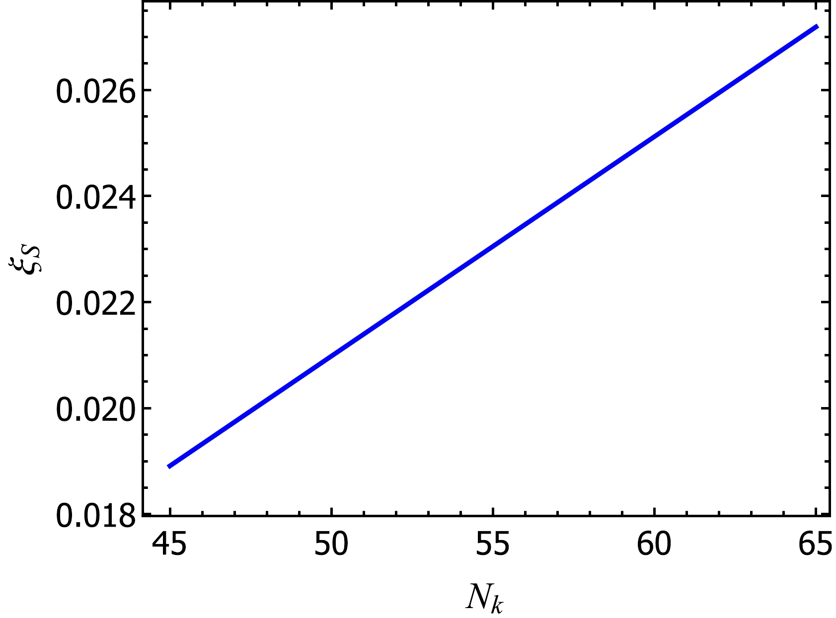
Figure 2. (color online) Non-minimal coupling parameter
$ \xi_s $ determined using Eq. (11) with$ \lambda_S=10^{-13} $ , varying as a function of$ N_k $ . The parameter$ \xi_s $ exhibits a rough proportionality to$ N_k $ , but it experiences negligible variation despite changes in$ N_k $ .The evolution of the number density of S- and h- particles obtained through the LATTICEEASY simulation are shown in Fig. 3. Note that the Higgs field begins to emerge as the inflaton starts its decay process. However, the decay of the inflaton does not strictly start immediately after inflation ends. This implies that particle production might be observable even before the end of inflation. [57] At the beginning of evolution, the particle number density increases exponentially. When the conformal time τ (
${\rm d}\tau=\dfrac{\sqrt{\lambda_S}S_0 }{a}{\rm d}t$ , where$S_0= S(\tau=0)$ ) is about 130, both particles almost reach the maximum number density and then slowly change, which indicates that the evolution of the universe transitions from preheating to reheating.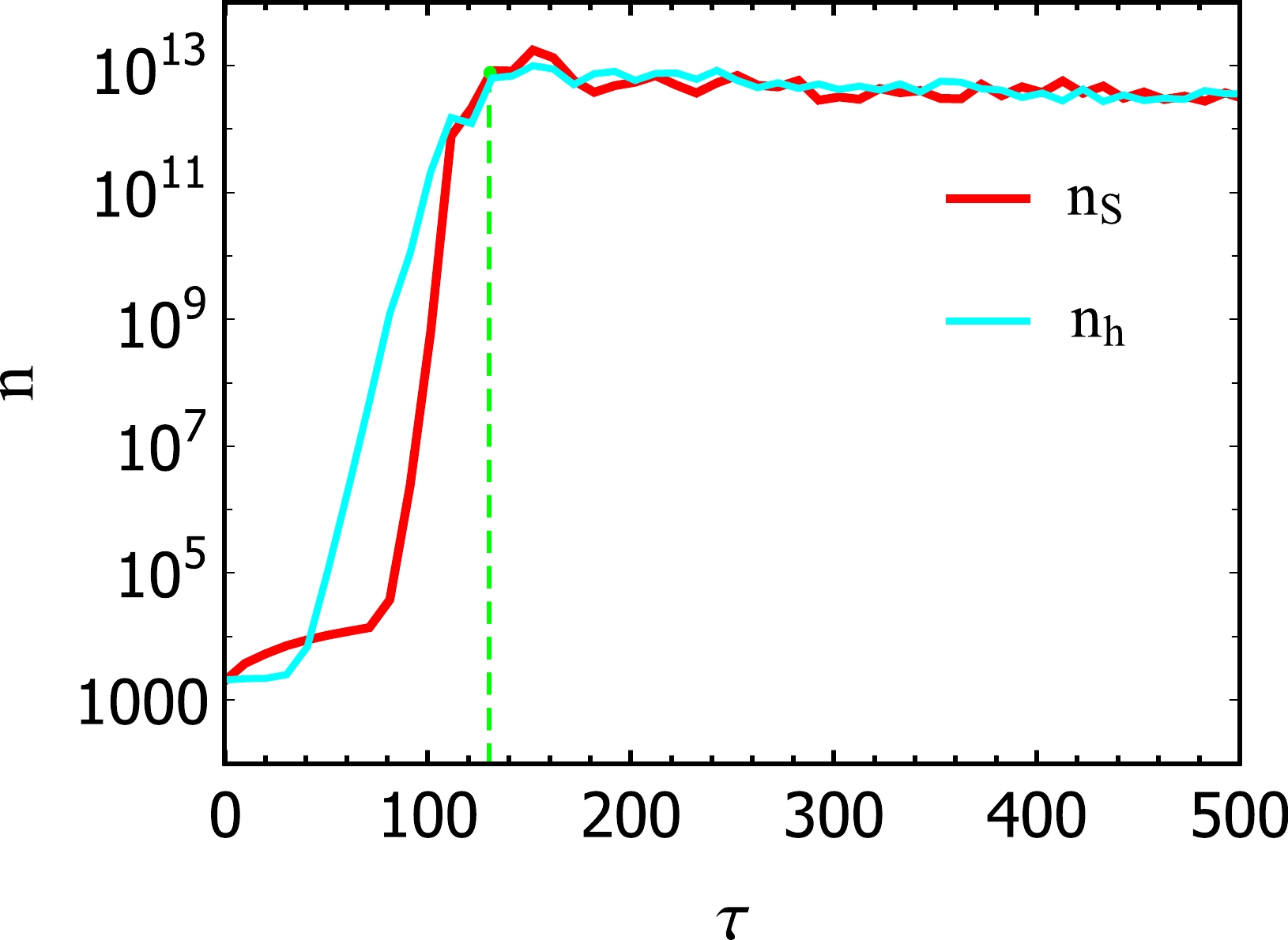
Figure 3. (color online) Evolution of number density of S- and h- particles, where the red and blue lines represent S- and h- particle number densities, respectively, and the green dashed line represents the end point of preheating.
The physics underlying this phenomenon can be explained as follows: when the slow-rolling condition is upset, the inflaton soon tumbles to the lowest point of potential and oscillates periodically around the lowest point, which causes the equation of motion of the h-field to become a Lame equation.
Parameter resonance for the h-field will emerge in some scenarios, which further cause an exponential increase in the h-particle number, whereas the h-particle decay produces a significant backreaction for S-particles, and the S-particle number density increases exponentially.
When the conformal time is about 130, the amplitude of the S-field oscillation decreases, which results in the weakening or even disappearance of the parametric resonance effect of the h-field; thus, the h-particle number density no longer increases, and, in the same conformal time, the backreaction effect disappears and the S-particle number density does not increase.
The variation in the scale factor over conformal time is shown on the left-hand side of Fig. 4. The end conformal time of the preheating obtained through the simulation of particle number density evolution is about 130, and the corresponding scale factor is
$a_{\rm end}\approx70$ , whereas the value of the scale factor at the beginning of the preheating is$a_{\rm star}=1$ . Thus, we can calculate the preheating e-folding number as$N_{\rm pre}=\ln[a_{\rm end}/a_{\rm star}]\approx 4.25$ .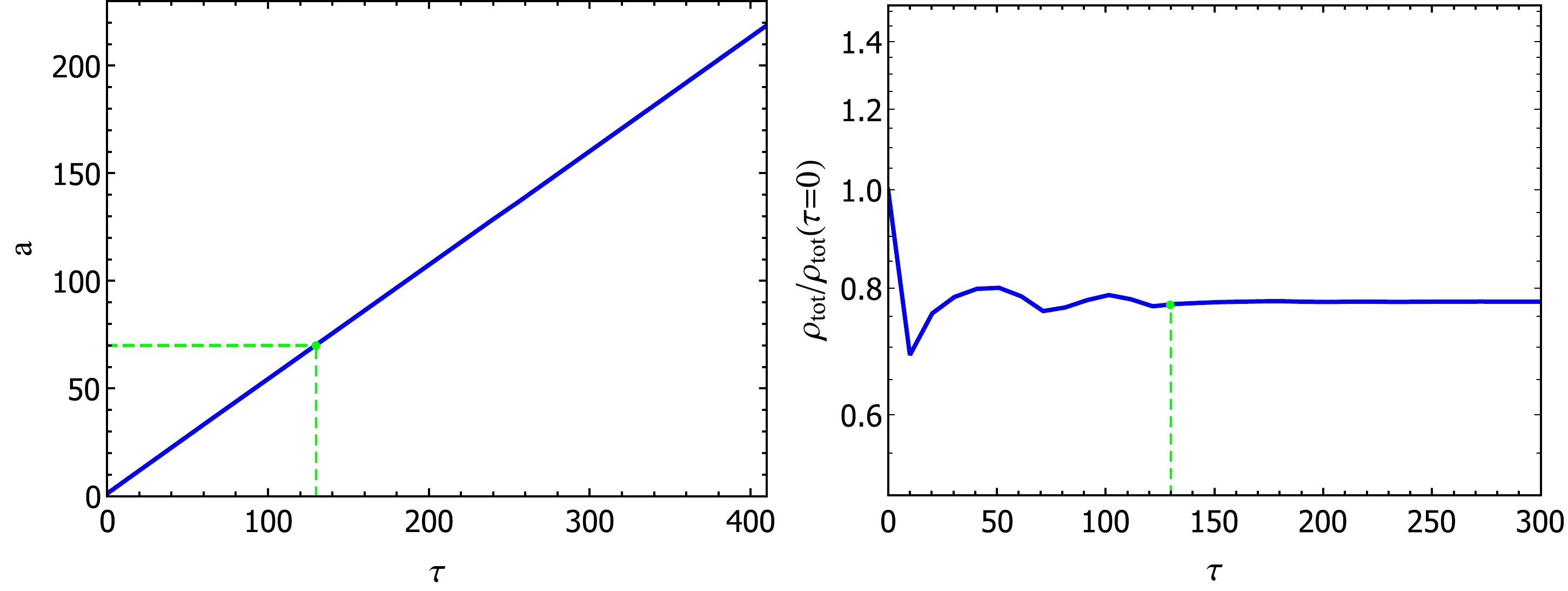
Figure 4. (color online) Evolution of the scale factor and total energy density for the left and right panels, respectively.
The evolution of normalized energy density
$\rho_{\rm tot}(\tau) / \rho_{\rm tot}(\tau=0)$ with respect to conformal time (τ) is shown on the right-hand side of Fig. 4, where the green dot is the ended energy of preheating according to Fig. 4 (left). Note that$\rho_{\rm tot}(\tau=0) = \rho_{\rm end}$ and$\rho_{\rm tot}(\tau=130) = \rho_{\rm pre}$ . Therefore, at$ \tau=130 $ , the y-label of Fig. 4 is represented as$\rho_{\rm tot}(\tau= 130) / \rho_{\rm tot}(\tau=0) \approx 0.77$ , i.e.,$\rho_{\rm pre} / \rho_{\rm end} = \gamma \approx 0.77$ . This simulation result differs significantly from the assumption ($ \gamma\approx10^3 $ or$ 10^6 $ ) in Ref. [38, 39]. -
Figure 5 shows the relationship between
$N_{\rm pre}$ and scalar spectral index ($ n_s $ ). The figure indicates that$N_{\rm pre}$ increases with the state parameter ω. After combining the Planck prediction of$ n_s $ with the LATTICEEASY simulation, we observe that the model has a feasible parameter space. The feasible range of ω is$ 1/4 $ to 1, and the corresponding$ n_s $ range is$ [0.9607, 0.9623] $ .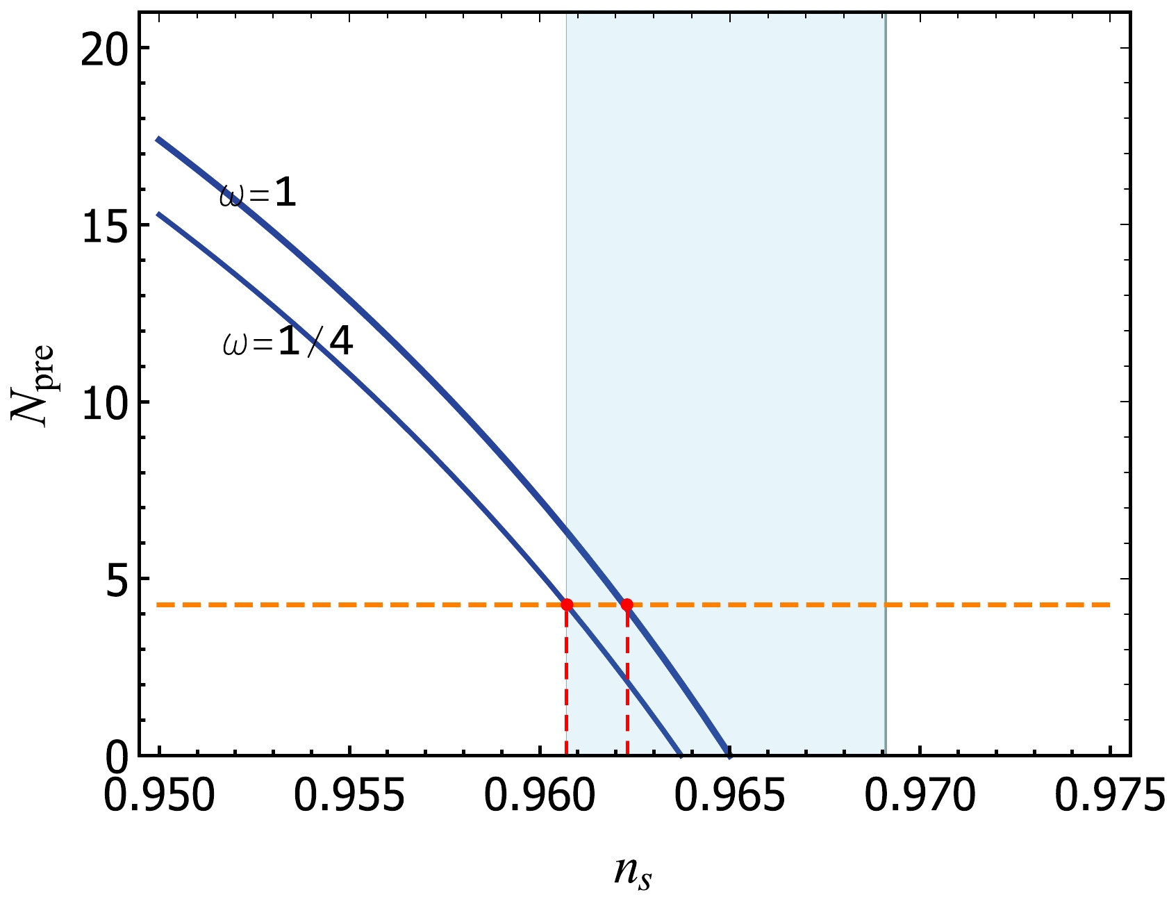
Figure 5. (color online) Relation between the scalar spectral index (
$ n_s $ ) and e-folding number of inflation ($ N_k $ ), where the cyan shaded is the feasible area of the Planck limit [4], the orange dashed line is the$N_{\rm pre}$ value obtained using the LATTICEEASY simulation, and the blue lines are calculated using Eq. (15), where the potential derived from the scalar inflation model and energy ratio γ is obtained through the LATTICEEASY simulation.The relation between
$ n_s $ and r is shown in Fig. 6. Note that the blue line between the red and cyan points is the feasible space of the LATTICEEASY simulation prediction obtained from Fig. 5. Therefore, the feasible parameter range of r can be obtained, i.e.,$ r\thicksim[ 3.9\times10^{-4}, 4.3\times10^{-4}] $ .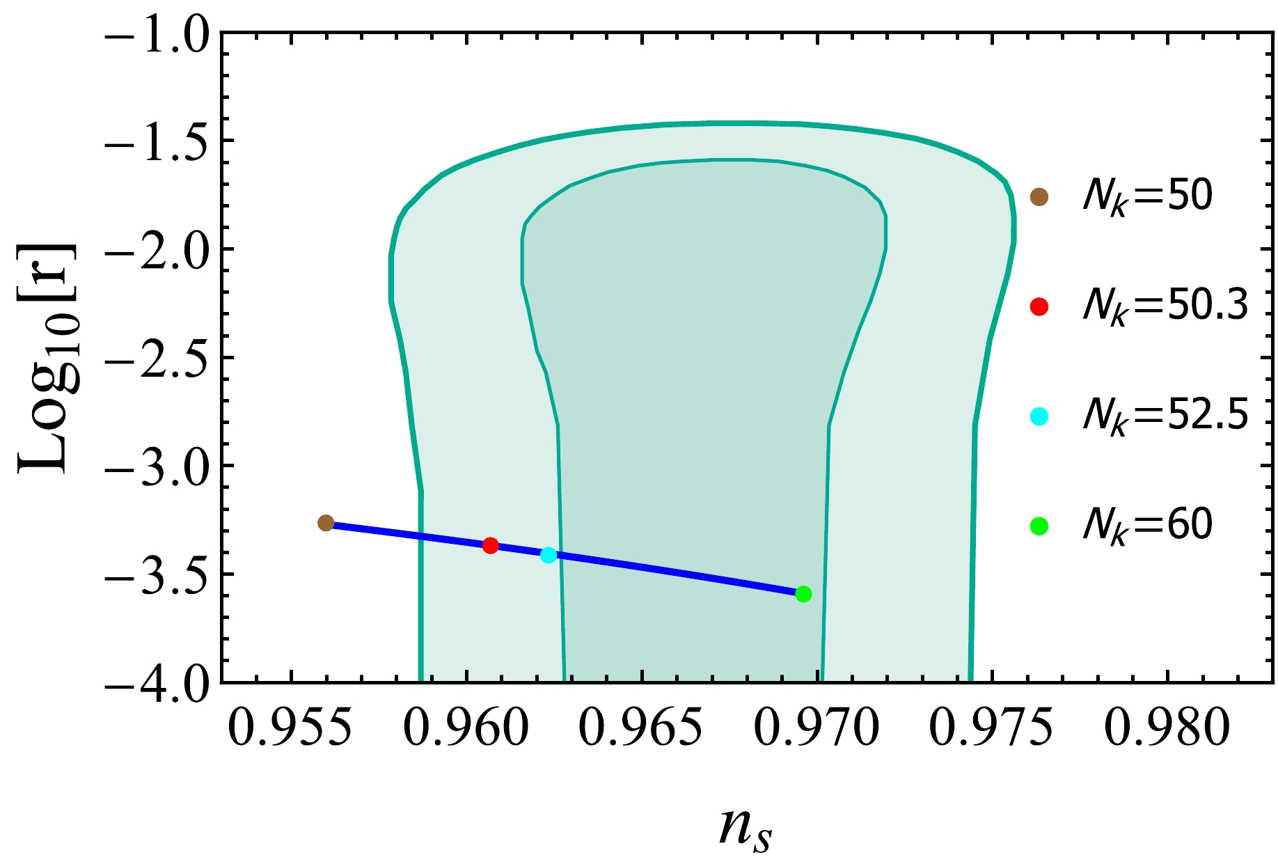
Figure 6. (color online) Relation between the scalar spectral index (
$ n_s $ ) and tensor-to-scalar power ratio (r), where the blue line is our theoretical prediction for$ N_k $ from 50 to 60, the green areas are the Planck limits, and the brown, red, cyan, and green points correspond to$ N_k= $ 50, 50.3, 52.5, and 60, respectively.To illustrate the, we list the fixed couplings of the scalar inflation model and the LATTICEEASY predictions in Table 1. Using the same strategy, we can test other model parameters.
γ $N_{\rm pre}$ 

w $ n_s $ 

$ N_k $ 

$ r\times 10^{-4} $ 

$ 0.77 $ 

$ 4.25 $ 

$ [1/4,1] $ 

$ [0.9607,0.9623] $ 

$ [50.3,52.5] $ 

$ [ 3.9, 4.3] $ 

Table 1. LATTICEEASY simulation predicts with
$ \lambda_S=10^{-13} $ ,$ \lambda_{Sh}=2\times10^{-11} $ , and$ \lambda_{h}=8\times10^{-12} $ . -
In this paper, we study non-minimum coupled real scalar inflation model using the preheating phenomenon simulated using LATTICEEASY. During inflation, the S-field has a crucial role in driving the expansion of the universe, with its quartic term dominating the dynamics of inflation. Interestingly, we find that the evolutionary behavior of the inflationary potential remains unaffected by the coupling coefficient of the model. Furthermore, the predictions of important quantities derived from the model are independent of this coupling coefficient.
Consequently, the tensor-to-scalar power ratio (r) and scalar spectral index (
$ n_s $ ) predicted using Planck observations do not impose constraints on the coefficients of the model. However, by leveraging the relationship between preheating and inflation, the preheating process simulated using LATTICEEASY provides a valuable avenue to address this problem effectively.We specifically investigate the constraint of inflation using the simulated preheating process, using the couplings
$ \lambda_S=10^{-13} $ ,$ \lambda_{Sh}=2\times10^{-11} $ , and$ \lambda_{h}=8\times10^{-12} $ as illustrative examples. By employing LATTICEEASY, we accurately reproduce the preheating dynamics within the scalar inflation model. With the introduction of LATTICEEASY, we have reproduced the preheating process of the scalar inflation model and obtained the particle number density evolution during the preheating process. Additionally, we have deduced the end conformal time value of preheating. At the same conformal time, the e-folding number of preheating ($ N_{\rm pre} $ ) and energy ratio (γ) are deduced by combining the simulated evolution of the scale factor and energy density, respectively.By exploiting the relationship between preheating and inflation, we present the variation in
$ N_{\rm pre} $ with$ n_s $ in Fig. 5, enabling us to deduce the range of w and$ n_s $ . Furthermore, by exploring the connection between$ n_s $ and$ N_k $ , as well as that between$ N_k $ and r, we can obtain constraints on the ranges of$ N_k $ and r. This implies that the preheating simulations conducted using LATTICEEASY can effectively predict$ n_s $ , r, and$ N_k $ , enabling restrictions on scalar inflation models. Furthermore, this strategy can be extended to effectively constrain models involving the inflaton dark matter model, as well as the interplay between inflation and dark matter models.
Constraints on real scalar inflation from preheating using LATTICEEASY
- Received Date: 2024-01-15
- Available Online: 2024-06-15
Abstract: In this paper, we undertake a detailed study of real scalar inflation using LATTICEEASY simulations to investigate preheating phenomena. Generally, the scalar inflation potential with non-minimal coupling can be approximated using a quartic potential. We observe that the evolutionary behavior of this potential remains unaffected by the coupling coefficient. Furthermore, the theoretical predictions for the scalar spectral index (


 DownLoad: