-
The search for dark matter (DM) [1−3] is a highly active research area in astroparticle physics. Among the various experimental approaches [4−12], dual-phase xenon time projection chamber (TPC) based experiments have been recognized as highly sensitive for detecting cold DM particles within the mass range of approximately 10 GeV/c
$ ^2 $ to TeV/c$ ^2 $ . PandaX-4T [10], located in the China Jinping Underground Laboratory (CJPL) [13, 14], is a typical experiment of this kind. PandaX-4T employs a cylindrical dual-phase xenon TPC with a sensitive volume measuring approximately 1.2 meters in diameter and 1.2 meters in height. The TPC is equipped with 368 3-inch photomultipliers (PMTs), 169 and 199 of which are distributed at the top and bottom of the PMT array, respectively. The TPC detects and measures the prompt scintillation signal (S1) and the subsequent amplified proportional scintillation signal (S2), which arises from the delayed ionization signals. By analyzing the time difference between the S1 and S2 signals, as well as the spatial distribution of the PMT hits associated with the S2 signal, we are capable of reconstructing the vertical and horizontal positions of the interaction vertex, respectively. Accurate 3-D position reconstruction and the determination of the S2/S1 ratio are crucial in particle discrimination within the TPC detector. This discrimination capability is important as it greatly reduces the effective background for DM direct searches.To interpret the DM search results in PandaX-4T, precise models for the low-energy background and DM signal are crucial. A critical component of the low-energy models is the reconstruction of the S1 and S2 signals. This reconstruction process involves various steps such as peak identification, pulse classification, and clustering. To accurately evaluate the efficiency and potential biases inherent in the software reconstruction, it is essential to obtain pure events that faithfully represent the desired physical signal. However, acquiring pure samples from the recorded reconstructed data is challenging because the recorded data have already been influenced by the effects of the software signal reconstruction inefficiency and biases. To address this challenge, a dedicated waveform simulation (WS) framework that generates synthetic data waveforms has been developed for PandaX-4T. The WS framework incorporates our best understanding of the processes involved in the generation, collection, and reconstruction of the S1 and S2 signals, as well as the accompanying sources of noise, such as dark counts, PMT after-pulsing, and impurity photoionization. In addition, the extensive samples generated by the WS can be utilized to train machine learning and deep neural network algorithms, which can further enhance background rejection capabilities.
This manuscript presents a detailed account of WSs employed in various scientific studies conducted using the PandaX-4T data to search for weakly interacting massive particles (WIMPs) [10], detect solar
$ ^8 $ B neutrinos [15], investigate light dark matter particles [16], etc [17, 18]. Section II of the manuscript elucidates the details of simulating the S1 and S2 pulses, as well as incorporating various sources of noise into the simulation process. Section III presents a comparison between simulation and real data, wherein critical variables such as signal width, pattern, and charge are evaluated. Finally, Section IV summarizes the work and discusses future perspectives. Similar works of other experiments can be found in Ref. [19]. -
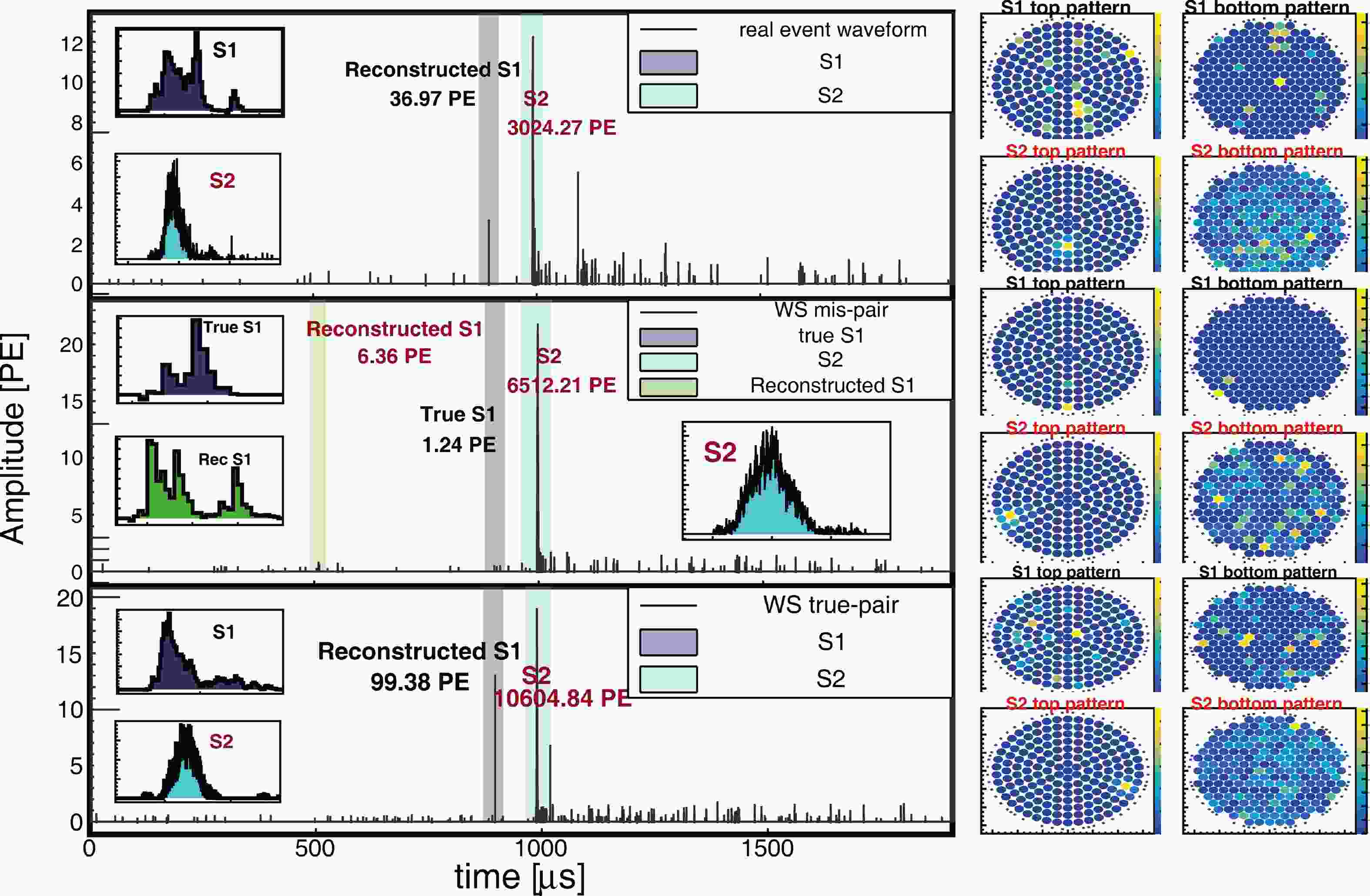
The simulated event waveforms in a WS further undergo the software processing and reconstruction chain that is used for data processing and analysis in PandaX-4T to ensure that the efficiency and bias of the simulated waveforms align with the observed data. WSs employ a semi-data-driven approach to simulate the S1 and S2 waveforms. The most fundamental segments of the S1 and S2 signals (hit and single-electron waveforms) are randomly selected from real data and then randomly reassembled to form simulated signals. Additionally, WSs take into account various spurious pulses, including noise, dark counts, PMT after-pulsing, and delayed afterglow after a large S2 pulse arising from impurity ionization and delayed electron effects. The high level characteristics of the simulated and real data are then compared to validate the modeling and prediction efficacies. To illustrate, two simulated waveforms are presented in the middle and bottom panels of Fig. 1. The bottom panel demonstrates successful identification of the S1 and S2 signals, albeit with a slight difference in the reconstructed charge values with respect to the true charge due to fluctuations in the reconstruction steps and interference from spurious pulses. In contrast, the middle panel exhibits complete misidentification of the S1signal, indicating a potential inefficiency in the software signal reconstruction process.
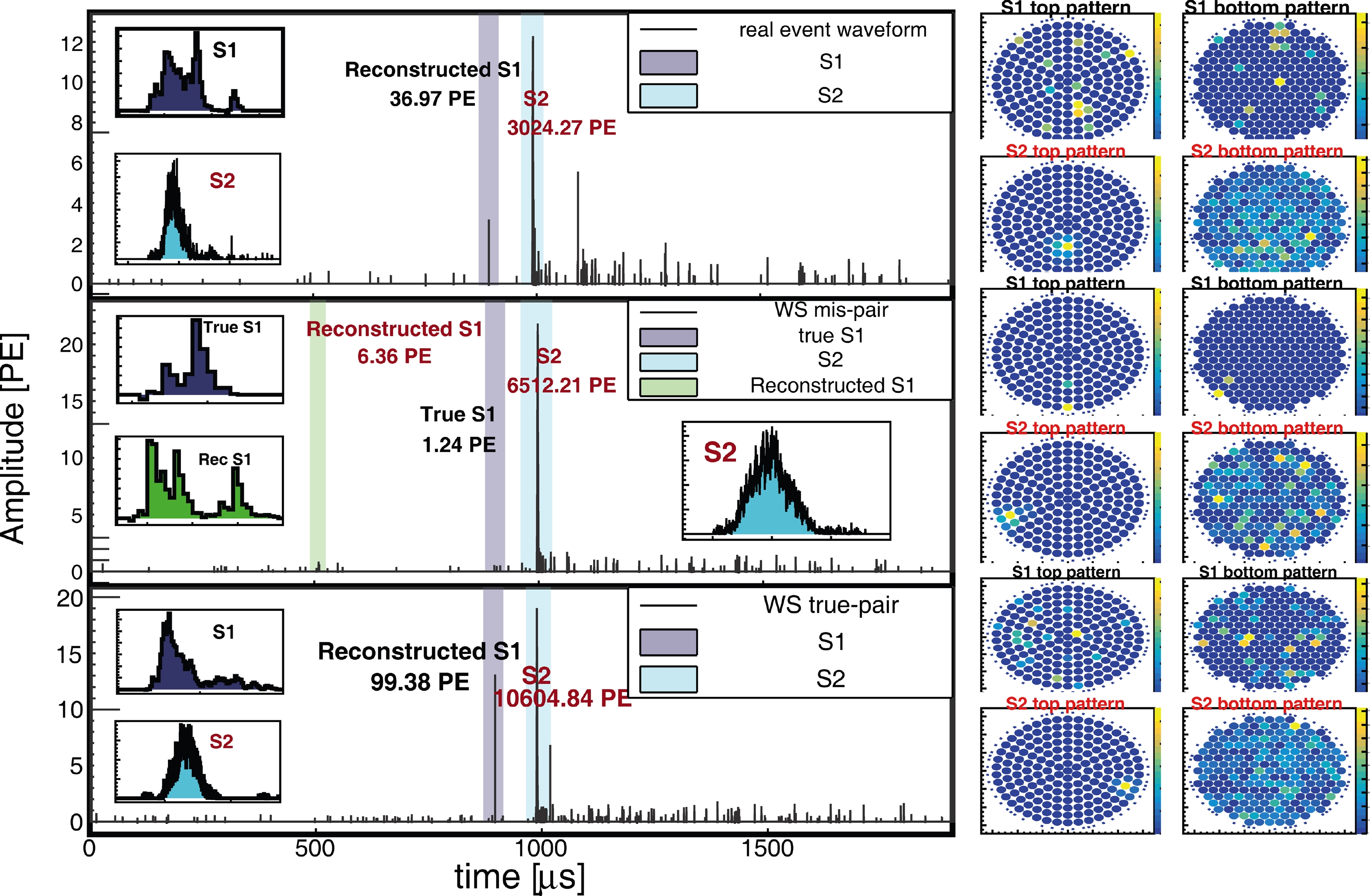
Figure 1. (color online) Three waveforms corresponding to events with similar drift times. Top panel represents a recorded data waveform. Middle panel shows a simulated waveform, where the true
$ S1 $ signal is overshadowed by a noise$ S1 $ signal with a slightly higher charge. Bottom panel displays a simulated waveform, where the$ S1 $ and$ S2 $ signals are correctly identified. Gray, green, and cyan shaded regions represent time windows associated with true$ S1 $ , misidentified$ S1 $ , and true$ S2 $ signals, respectively. Reconstructed charge of identified$ S1 $ and$ S2 $ signals are displayed in panels. For enhanced detail, inset panels provide zoomed-in views of$ S1 $ and$ S2 $ signals. Hit patterns of main$ S1 $ and$ S2 $ signals are shown in right columns. -
The S1 signal represents the prompt scintillation signals detected in the TPC detector, arising from the interaction of particles with the xenon shell electrons or nucleus. The S1 signal exhibits a relatively short time scale, typically ranging from a few tens of nanoseconds to approximately 100 nanoseconds, which originates from light propagation in the TPC. The shape of the S1 pulse is influenced by the PMT signal shaping, decay time profile of singlet and triplet xenon dimers, and propagation of photons within the TPC. The ratio between the singlet and triplet dimer decays differs slightly between electronic recoils (ERs) and nuclear recoils (NRs). In ER events, where the incoming particle interacts with the xenon shell electrons, this ratio tends to be slightly higher compared to NR events [20, 21], where the interaction occurs with the xenon nucleus. However, the difference in pulse shapes between ER and NR events is obscured as a consequence of photon propagation effects, such as photon Rayleigh scattering and the reflection on the liquid surface and TPC wall.
To simulate the S1 waveform, a data-driven approach is adopted. In this approach, the S1 signals from
$ ^{220} $ Rn [22] and neutron calibration data, including a$ ^{241} $ AmBe radioactive source and Deuteron-Deuteron (DD) neutron generator, are utilized to simulate the S1 waveforms corresponding to the ERs and NRs, respectively. The S1 signals with a charge of 2–200 photoelectrons (PE) and 2–150 PE were selected as the ER and NR S1 pools, respectively. It was observed that the hit distribution among the PMTs for the majority of the S1 signals that occurred in the fiducial volume was quite uniform owing to Rayleigh scattering and reflection on PTFE. Within the charge levels of the S1 pools, the S1 waveforms consisted of single-photon hits that were distributed among multiple PMTs. The probability of two hits occurring on same PMT was negligible. Additionally, the time response of the PMTs to a single hit was within appoximately 10 ns, while the time spread due to photon propagation was approximately 40 ns. Two hits occurring on same PMT were likely distinguishable by time. The single-photon hit waveform on a PMT is depicted in the left panel of Fig. 2. Based on the above facts, a simulation of the S1 waveform was performed by sampling the hits of an S1 pool. The S1 pool was required to have the same event position as the simulated S1 signal (transverse distance$ < $ 5 cm and vertical distance$ < $ 8 cm). Figure 3 shows an example of a simulation. An S1 pool with 19 hits was used to simulate an S1 signal with 13 hits, and 68% of the pooled hits were sampled to form the simulated S1 signal. This data-driven approach naturally takes into account the position-dependent characteristics of the S1 pulse time profile resulting from light propagation and variations of the PMT characters, such as the gains and SPE resolution. The right panel of Fig. 2 displays the hit time distributions of the S1 signals in the ER and NR calibration data from various Z positions. The differences in the shape of the waveforms arises from the differences in the spatial position distributions in the ER and NR calibration data.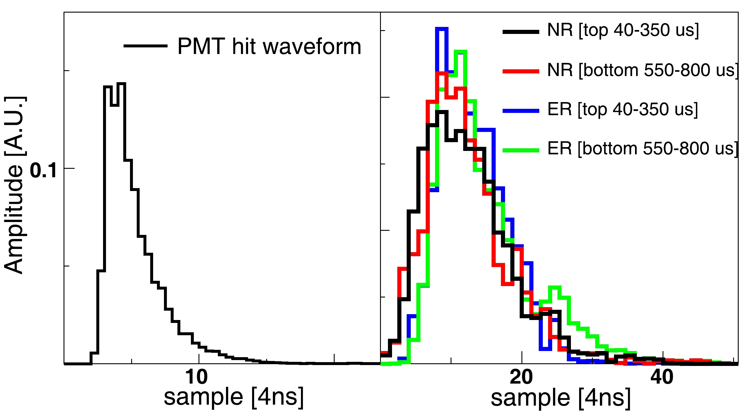
Figure 2. (color online) Single PE waveform (left) and time distributions (right) of
$ S1 $ hits. Blue, orange, and red solid lines in right panel represent distributions from$ ^{220} $ Rn,$ ^{241} $ AmBe, and DD calibration data, respectively.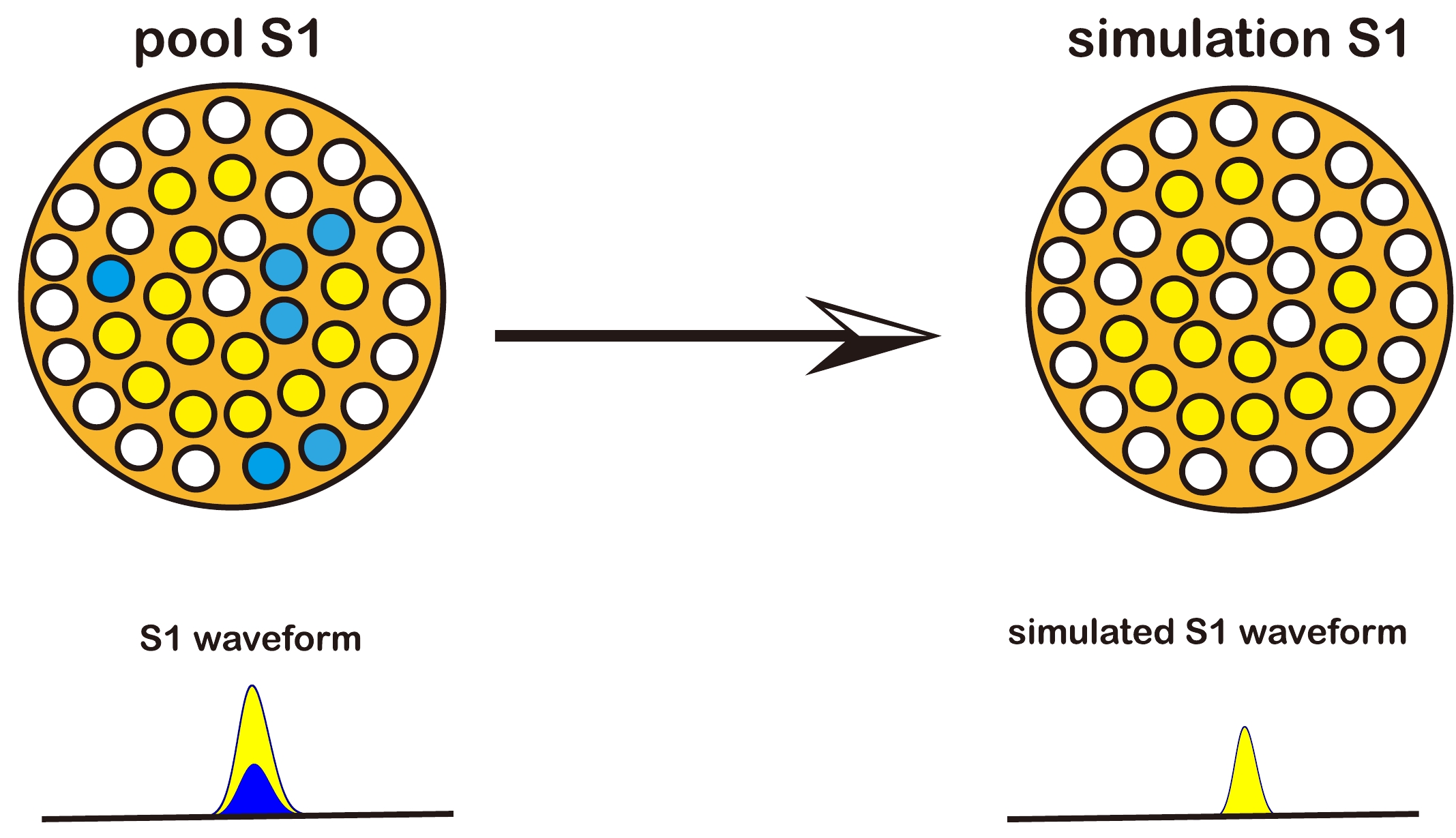
Figure 3. (color online) Example of
$ S1 $ waveform simulation.$ S1 $ pool has 19 hits and simulated$ S1 $ signal is required to have 13 hits. Six hits from$ S1 $ pool are randomly selected for dropping, and the rest are taken as simulated$ S1 $ signal. Pattern and waveform of dropped hits are in blue in the left panel. -
The S2 signal corresponds to the detection of proportional scintillation light emitted by the drifted electrons when they reach the gaseous xenon layer between the anode and gate electrodes in the TPC detector. The shape of the S2 pulse is predominantly determined by two factors: the diffusion of electrons during their drift from the interaction vertex to the gaseous xenon layer, and the subsequent travel within the gaseous layer. The longitudinal diffusion coefficient in liquid xenon has been experimentally measured to be approximately 30–40 cm
$ ^2 $ /s at an electric field of 100 V/cm [23]. To obtain accurate in-situ values for the longitudinal diffusion coefficient, measurements are performed using different calibration sources. Specifically, the 41 keV gamma line from the$ ^{83m} $ Kr calibration data, and the α decay events from$ ^{222} $ Rn are utilized. Figure 4 illustrates the 80%-CDF S2 width (defined as the length of time window that covers central 80% of the S2 charge) over drift time distributions for these events, and the mean 80%-CDF S2 widths as a function of drift time were used to calculate the respective longitudinal diffusion coefficients. The longitudinal diffusion coefficient$ D_L $ can be obtained by fitting the mean 80%-CDF S2 widths (denoted as$ \langle W_{S2}^{80} \rangle $ ) as a function of drift time by the relation: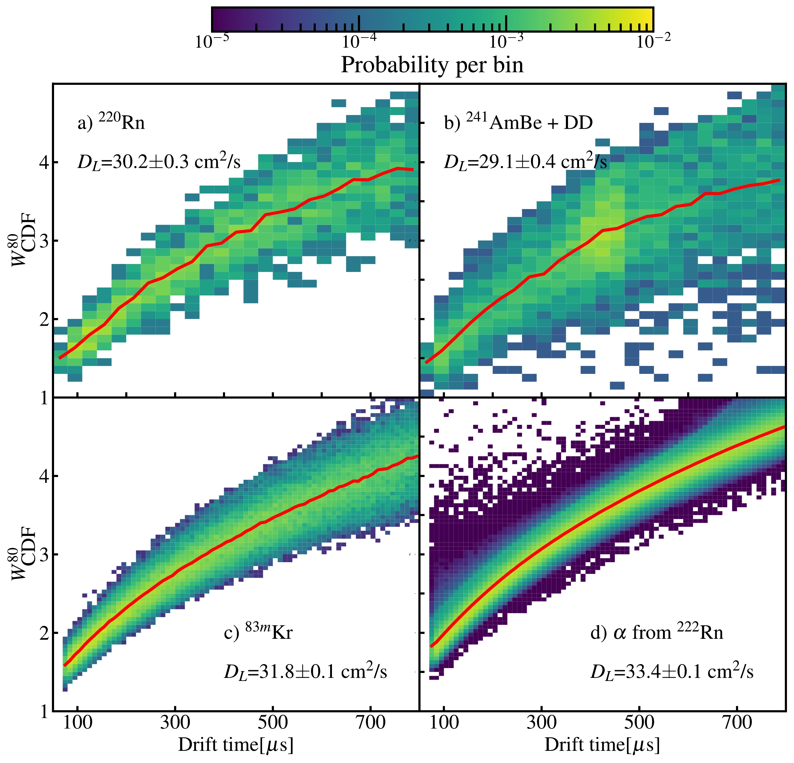
Figure 4. (color online) Normalized distributions of
$ W^{80}_{ \rm{CDF}} $ over drift time for four types of data: a)$ ^{220} $ Rn calibration, b) neutron calibration using$ ^{241} $ AmBe and DD, c)$ ^{83m} $ Kr calibration, and d) α events originating from$ ^{222} $ Rn impurities. Red solid lines represent distribution means.$ D_L $ values obtained from fitting the means using Eq. (1) are given in each panel.$ \langle W_{S2}^{80} \rangle = \frac{f^{80}}{\nu_d} \sqrt{2 D_L T + \sigma^2_0}, $

(1) where T is the drift time and
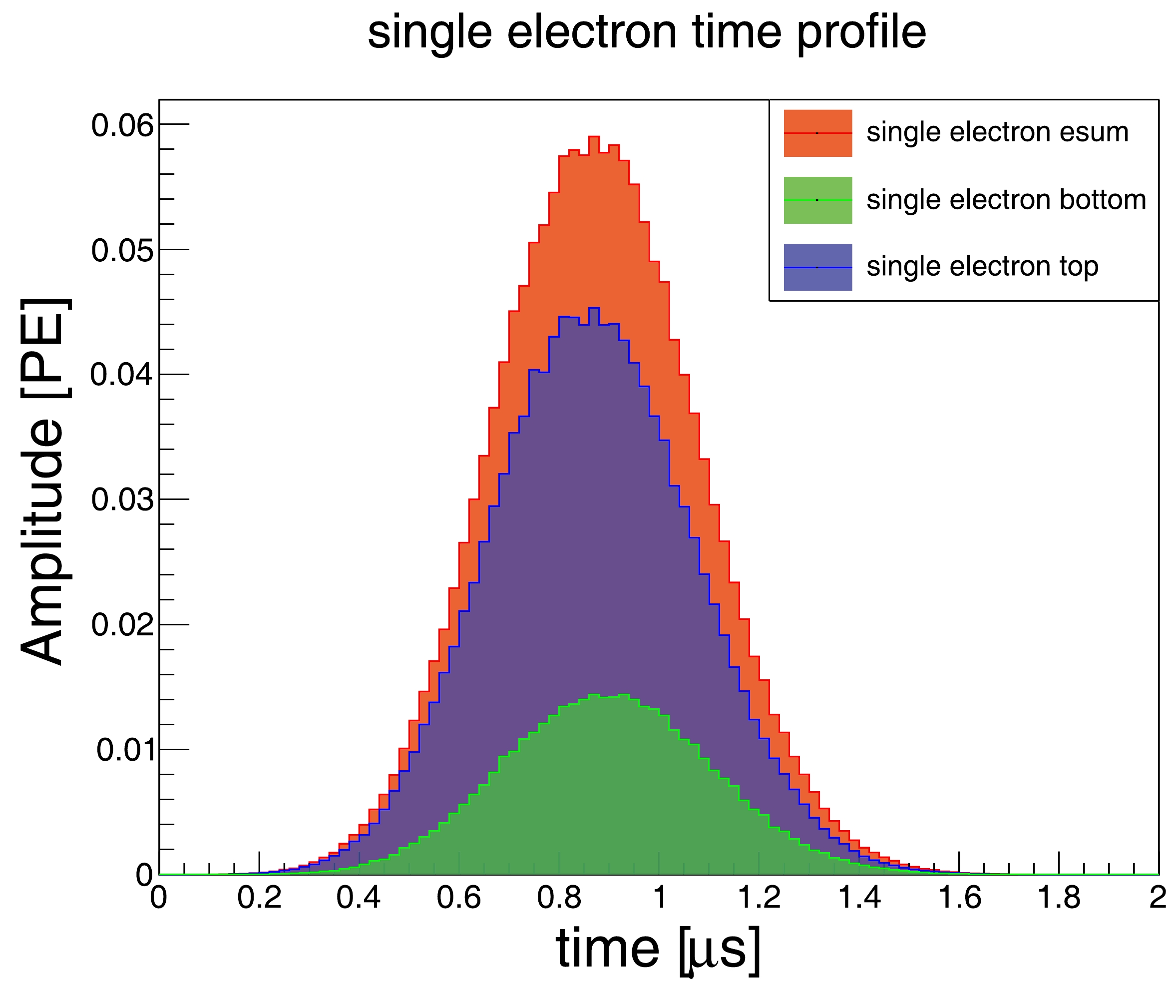
$ \sigma_0 $ is the standard deviation of the photon hit time in a single electron (SE) waveform.$ \sigma_0 $ is affected by the travel time of the electron in the gaseous xenon layer, and depends on the gas gap and electric field strength in the gap.$ \sigma_0 $ is calibrated to be 0.2 mm in Run0 of PandaX-4T.$ \nu_d $ is the drift velocity in LXe, which was set to 1.44 mm/μs. The factor$ f^{80}=2.56 $ is the conversion factor from the standard deviation to 80%-CDF width that assumes the S2 pulse shape is Gaussian. The best-fit$ D_L $ using low-energy data ($ ^{220} \rm{Rn} $ ,$ ^{241} $ AmBe, and DD) was systematically lower than the results obtained using the high-energy data ($ ^{83m} $ Kr and α from$ ^{222} $ Rn). This is due to the statistical bias of the S2 pulse width when the S2 charge is only caused by a few electrons. The variations observed in the best-fit diffusion coefficients obtained from high-energy α also suggest the potential presence of systematic effects in high-energy samples, such as PMT saturation. Consequently, the WS employes the diffusion coefficient from$ ^{83m} $ Kr calibration data. This coefficient agrees well with the width versus drift time distributions of the low-energy data, discussed later in the text. The time profile of electron travel within the gaseous xenon can be determined by analyzing the SE waveforms, as depicted in Fig. 5. The average SE waveforms shown in Fig. 5 are obtained by stacking the SE waveforms with the arrival time of their first hit set to zero. The electric field and decay characteristics of xenon dimers in the gaseous phase influenced the observed time profile.The SE waveforms from the data were reassembled to generate simulated S2 signals in the WS. To ensure compatibility of the (X, Y) positions between the simulated S2 signals and data, SE waveforms with reconstructed positions
$ R_0 $ within a certain range, specifically within 4 cm from the simulated position, were selected for the assembly process. This value was determined to efficiently match the pattern of the S2 signals (see Section III for more detail). Each selected SE pulse waveform was given a time shift before reassembly, to ensure that the simulated SE arrival times adhered to the diffusion principle in Eq. (1). Figure 6 shows an example of a waveform simulation for an S2 signal from a 2-electron signal. Two SE waveforms were sampled from the SE pool, with charges of 31.56 and 14.61 PE, respectively. We required the simulated S2 signal to have a z position of 47.2 cm, which results in a S2 CDF width of 2.56 μs. The two SE waveforms were given time shifts of –0.87 and 0.57 μs, respectively.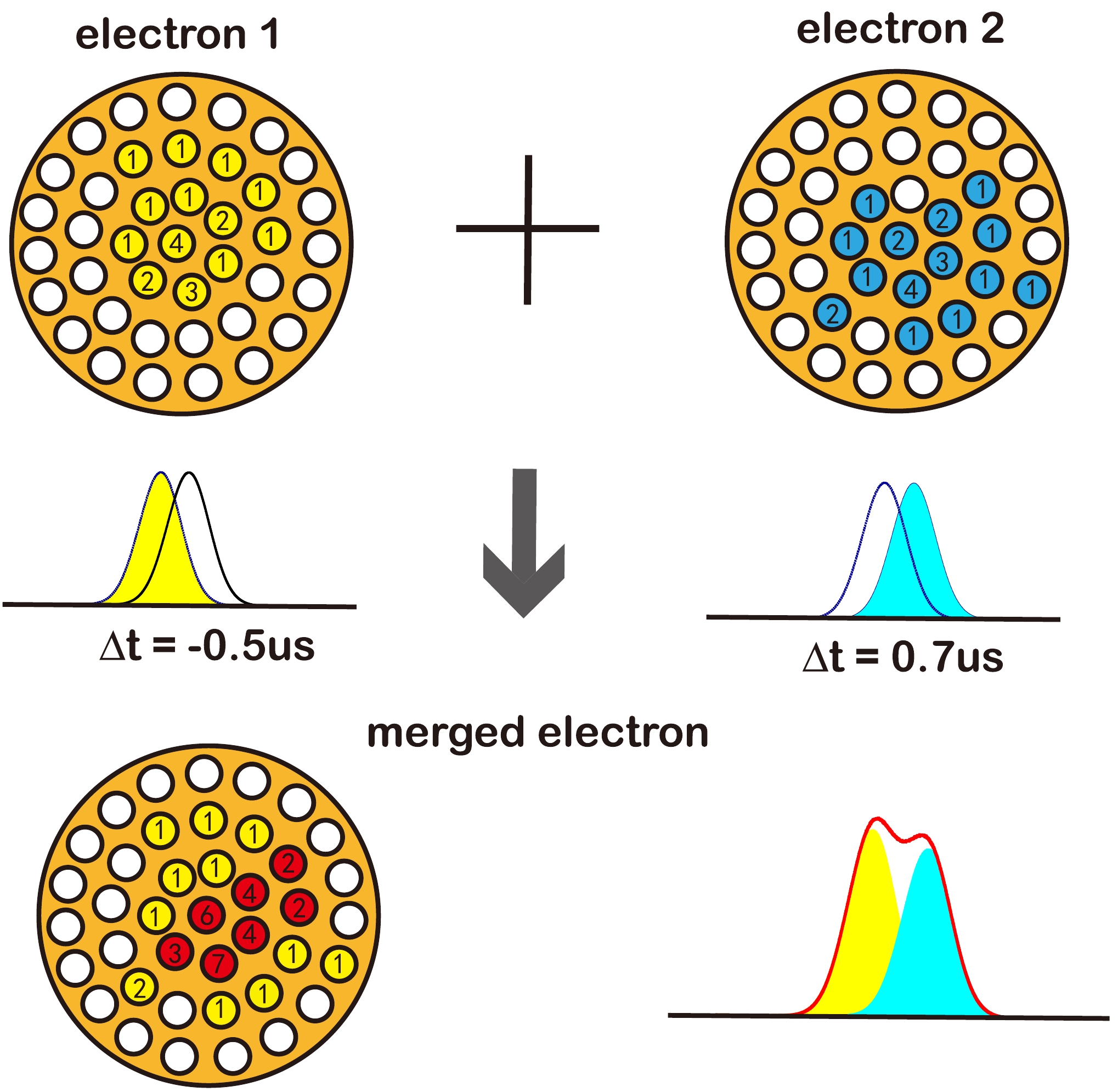
Figure 6. (color online) Example of S2 simulation. Two SE events were selected from SE pools. Their patterns and waveforms are shown in the upper panels. Time shifts were given to each SE waveforms and followed a Gaussian distribution, which is compatible with the diffusion of an event from Z = 47.2 cm. The pattern and waveform of the then merged simulated S2 signal are shown in the lower panel. The number given in the pattern plot represents the hit number seen by the PMT.
-
When a PMT detects light signals, residual gases in the PMT can become ionized owing to the acceleration of photoelectrons (PEs) [24−27]. These positively charged ions then drift back towards the photocathode of the PMT, causing the emission of additional PEs. Consequently, small delayed signals may appear after the main pulse. The majority of residual gases tend to be concentrated on the first dynode of the PMT, leading to characteristic and constant time delays for certain ions in the PMT response due to after-pulsing. The magnitude of the time delay is primarily proportional to the square root of the atomic mass over the ion charge of the gas molecule. Furthermore, the number of PEs that each residual gas ion can generate is dependent on the type of residual gas. In WSs, the number of PMT after-pulsing hits and the charge of each hit are sampled according to the average differential probability and mean charge of the PMT after-pulsing, respectively, as a function of the delay time, as shown in Fig. 7. The average probability of after-pulsing after each PE in the 3-inch PMTs utilized in the PandaX-4T experiment was approximately 3%.
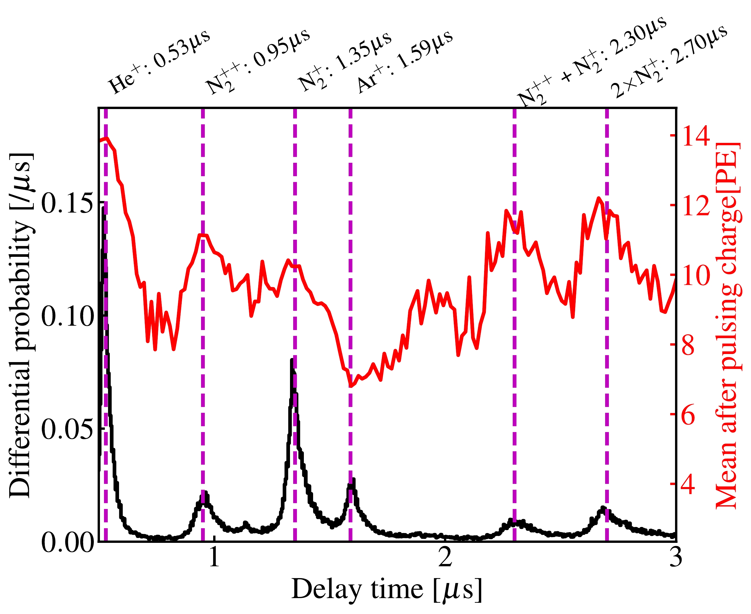
Figure 7. (color online) Differential probability of PMT after-pulsing as a function of delay time. After-pulsings caused by helium, nitrogen, and argon residual gases are most visible, and highlighted by the magenta dashed lines. Secondary after-pulsing of nitrogen is also indicated by magenta dashed lines. Red solid line shows the mean charge of after-pulsing after each single-PE.
-
In several LXe-TPC detectors, it has been observed that additional S2 signals appear subsequent to a large S2 signal [28−30], commonly referred to as delayed S2 signals or delayed electrons. The appearance of these delayed signals is attributed to various factors. One significant factor is the photoionization of the electrode metal. The electrons resulting from this photoionization process exhibit distinct drift times, as depicted in Fig. 8. Delayed electrons can also arise from the photoionization of electro-negative impurities (mainly oxygen) uniformly distributed within the detector. It is also speculated that impurities present in the LXe may "capture" and subsequently release drifting electrons [30], leading to delayed S2 signals. Other processes, such as electron trapping at the liquid-gas interface [31] and spontaneous electron emission from the electrode [32, 33], have also been proposed as potential contributors to the delayed S2 phenomenon. In the PandaX-4T experiment, a data-driven approach was employed to model the probability of delayed electron generation. By stacking selected S2 waveforms with a fixed reference time (e.g., the start of the waveform), the resulting stacked waveform was analyzed to give the production probability, as shown in Fig. 8. The correlation between the probability of the delayed electron production and the corresponding delay times was modeled empirically using a combination of two Gaussians and two exponential distributions. The Gaussian components represent delayed electrons originating from the gate and cathode electrodes. The mean delay time for the gate delayed electrons, extracted from the fit to the stacked waveform, was 3.2 μs. These values align with the expected behavior, assuming the liquid-gas interface is 5–8 mm above the gate. The delayed electrons from the cathode were negligible compared to other components. The two exponential distributions were found to adequately model delayed electrons resulting from impurity photoionization and electron delays caused by impurity or liquid surface trapping. The probabilities of generating one delayed electron per detected S2 photon were determined as 0.24 and 0.15%, respectively, for the gate photoionization and other aforementioned effects. In the WS, the number of delayed electrons were sampled based on these probabilities and the delay time distributions are shown in Fig. 8. The secondary photoionization caused by the primary photoionization was negligible and not implemented in the WS. Further adjustments to the photoionization probability were made to account for the presence of small S2 signals in the S2 waveform samples obtained from real data.
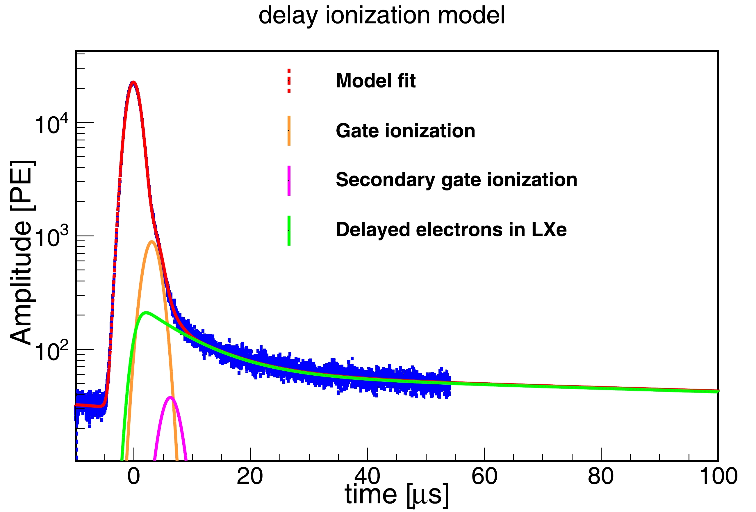
Figure 8. (color online) Average
$ S2 $ waveform (blue solid line). Red solid line shows a fit to the average$ S2 $ waveform, consisting of gate ionization (orange solid line) and delayed electron contribution from LXe (green solid line). The gate photoionization was generated from a fixed Z position and was modeled as Gaussian. The delayed electrons in LXe were modeled as the sum of two exponentials convoluted by a Gaussian. The Gaussian convolution represents time spread due to electrons traveling in the gas gap during proportional amplification. The$ S2 $ light of gate photoionization (magenta solid line) also further generated photoionization (secondary gate photoionzation). -
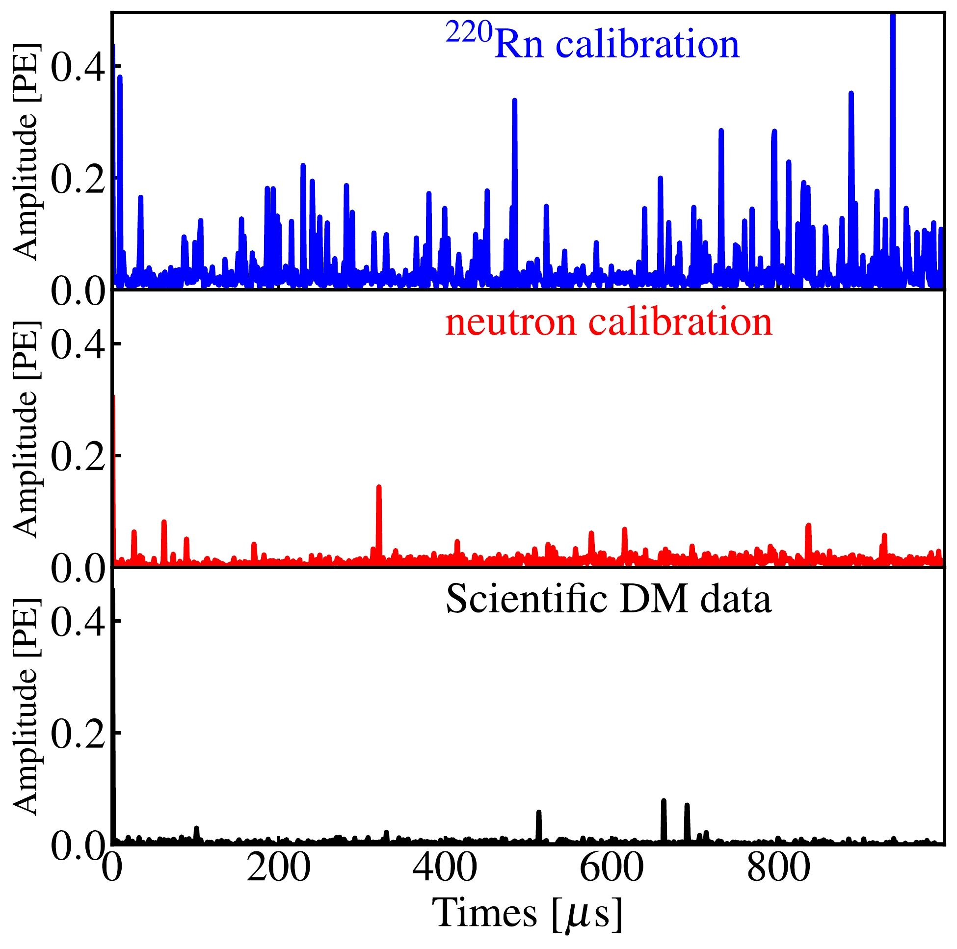
Apart from the aforementioned effects, it is important to consider the presence of noise and dark counts from the PMTs, as they can potentially overshadow the small S1 signals and lead to incorrect pairing. Noise mainly refers to spurious lights present in the TPC that are observed to follow a large S2 signal [34]. As the S2 rates increase in the calibration data, the corresponding noise rate also increase. To account for these sources of noise and dark counts, they were incorporated into the WS by stacking real segmented waveforms on top of the simulated waveform. These noise segments were randomly sampled from the 2-ms window preceding the identified S1 signal. The noise level appeared to have a correlation with the type of run conducted. Figure 9 displays selected segmented waveforms from scientific runs for the DM search, ER calibration, and NR calibration.
-
To evaluate the performance of the WS, a comparative analysis was performed by examining the distributions of key variables between the simulated samples and experimental data. These key variables were derived by subjecting the simulated waveforms to the same data processing algorithm employed in the PandaX-4T experiment. The variables selected for comparison can be classified into four distinct categories, with respect to S1 pulse shape, S2 pulse shape, pattern, and waveform "dirtiness". The description of these variables can be found in Table 1.
Category Symbol Description reference $ S1 $ -related

$ N^{ \rm{peak}}_{S1} $ 

Number of peaks of major $ S1 $ .

Figs. 10 and 12 $ Q_{S1} $ 

Total charge of major $ S1 $ .

$ h_{S1} $ 

Pulse maximum height of major $ S1 $ .

$ W_{S1} $ 

Difference of end and start times of major $ S1 $ pulse.

$ W_{S1}^{ \rm{FWHM}} $ 

Half-height width of major $ S1 $ .

$ W_{S1}^{ \rm{ten}} $ 

10%-height width of major $ S1 $ .

$ N^{ \rm{hit}}_{S1} $ 

Number of hits for major $ S1 $ .

$ N^{ \rm{cand}}_{S1} $ 

Number of candidate $ S1 $ signals in the event.

$ M^{ \rm{bot}}_{S1} $ 

Charge on most-fired bottom PMT of major $ S1 $ .

$ S2 $ -related

$ N^{ \rm{peak}}_{S2} $ 

Number of peaks of major $ S2 $ .

Figs. 11 and 13 $ Q_{S2} $ 

Total charge of major $ S2 $ .

$ W^{ \rm{FWHM}}_{S2} $ 

Half-height width of major $ S2 $ .

$ W^{ \rm{ten}}_{S2} $ 

10%-height width of major $ S2 $ .

$ h_{S2} $ 

Pulse maximum height of major $ S2 $ .

$ R_{ \rm{pre}S2} $ 

Fraction of charge in pre-maximum-height window to total of major $ S2 $ .

$ N^{ \rm{hit}}_{S2} $ 

Number of hits of major $ S2 $ .

$ W^{80}_{S2} $ 

$ S2 $ width containing 80% charge.

$ \sigma^{ \rm{hit}}_{S2} $ 

Standard deviation of charges of hits among PMTs of major $ S2 $ .

Pattern-related $ A_{S1} $ 

Top-bottom asymmetry of major $ S1 $ .

Figs. 14 and 15 $ A_{S2} $ 

Top-bottom asymmetry of major $ S2 $ .

$ F_{S1}^{ \rm{maxq}} $ 

Fraction of charge on most-fired PMT over total charge of major $ S1 $ .

$ F_{S2}^{ \rm{maxq}} $ 

Fraction of charge on most-fired PMT over total charge of major $ S2 $ .

$ \sigma^{ch}_{S1} $ 

Standard deviation of charges of fired PMTs of major $ S1 $ .

$ \sigma^{ \rm{CoG}}_{S2_b} $ 

Root-mean-square of hit PMT positions to center-of-gravity reconstructed position of major $ S2 $ .

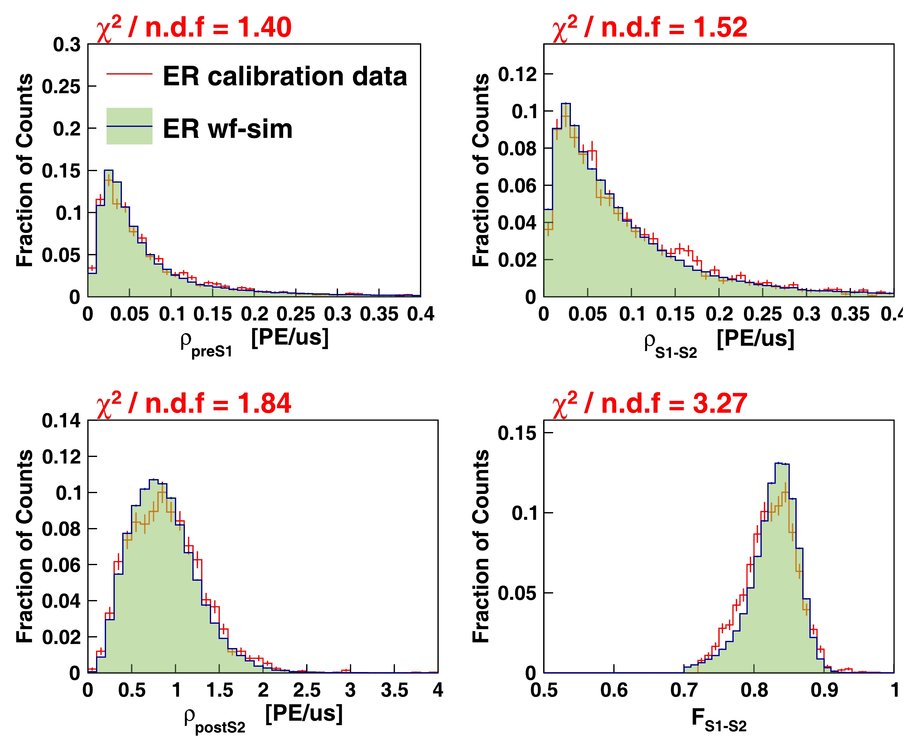
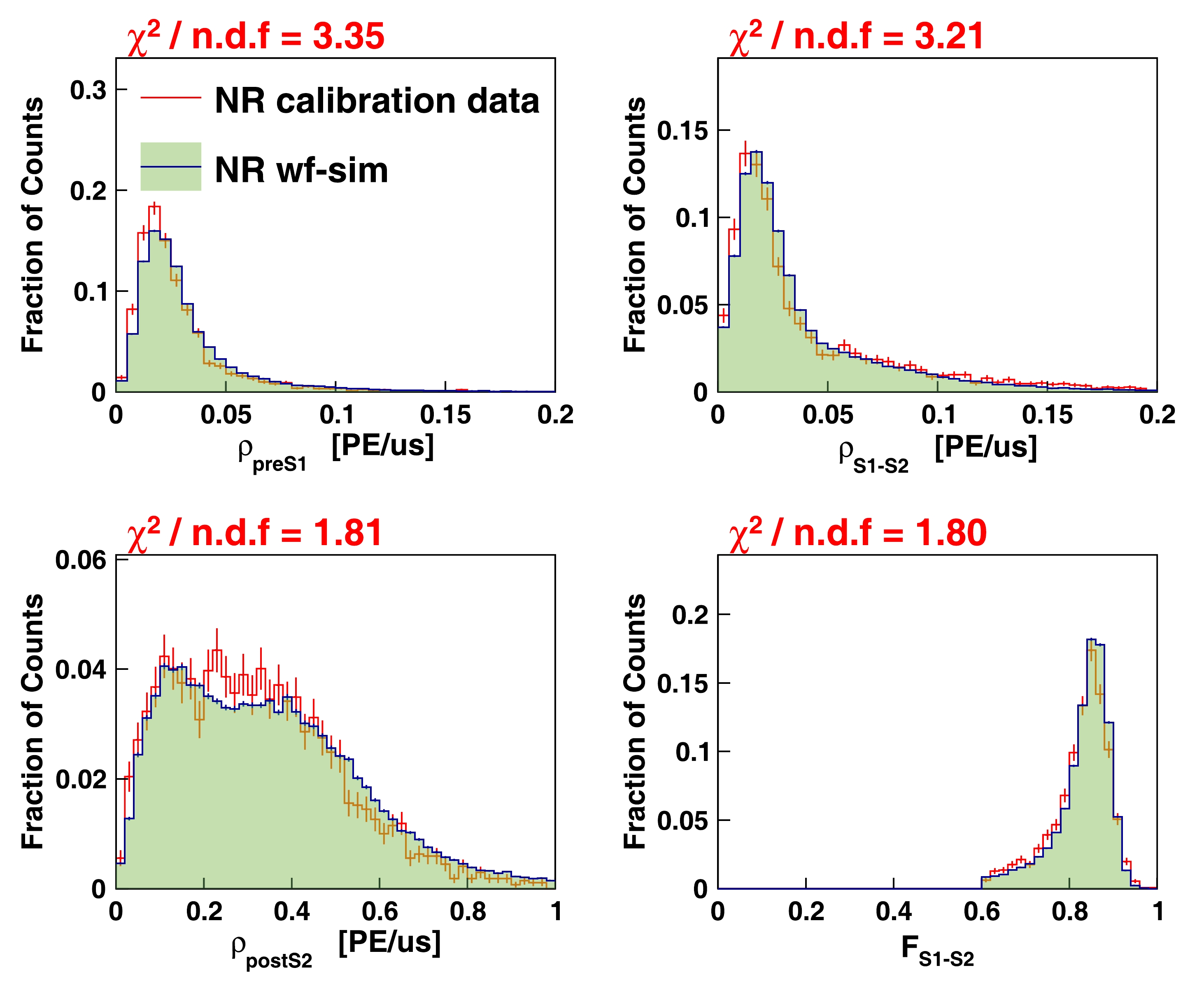
Waveform "dirtiness" $ \rho_{ \rm{preS1}} $ 

Charge density before major $ S1 $ .

Figs. 16 and 17 $ \rho_{S1-S2} $ 

Charge density inbetween major $ S1 $ and

$ S2 $ .

$ \rho_{ \rm{postS2}} $ 

Charge density after major $ S2 $ .

$ F_{ \rm{S1-S2}} $ 

Charge fraction of major $ S1 $ plus

$ S2 $ to total charge in event waveform.

Table 1. List of key variables used to compare the data and WS.
The comparison was conducted using the
$ ^{220} $ Rn and neutron calibration data for ER and NR, respectively. The data selections that were used for DM search [35] were applied. To mitigate the potential influence arising from correlations between the key variables and parameters such as S1 charge, S2 charge, and event position, it is necessary to ensure that the distributions of S1, S2, and position in the WS and data samples are compatible. -
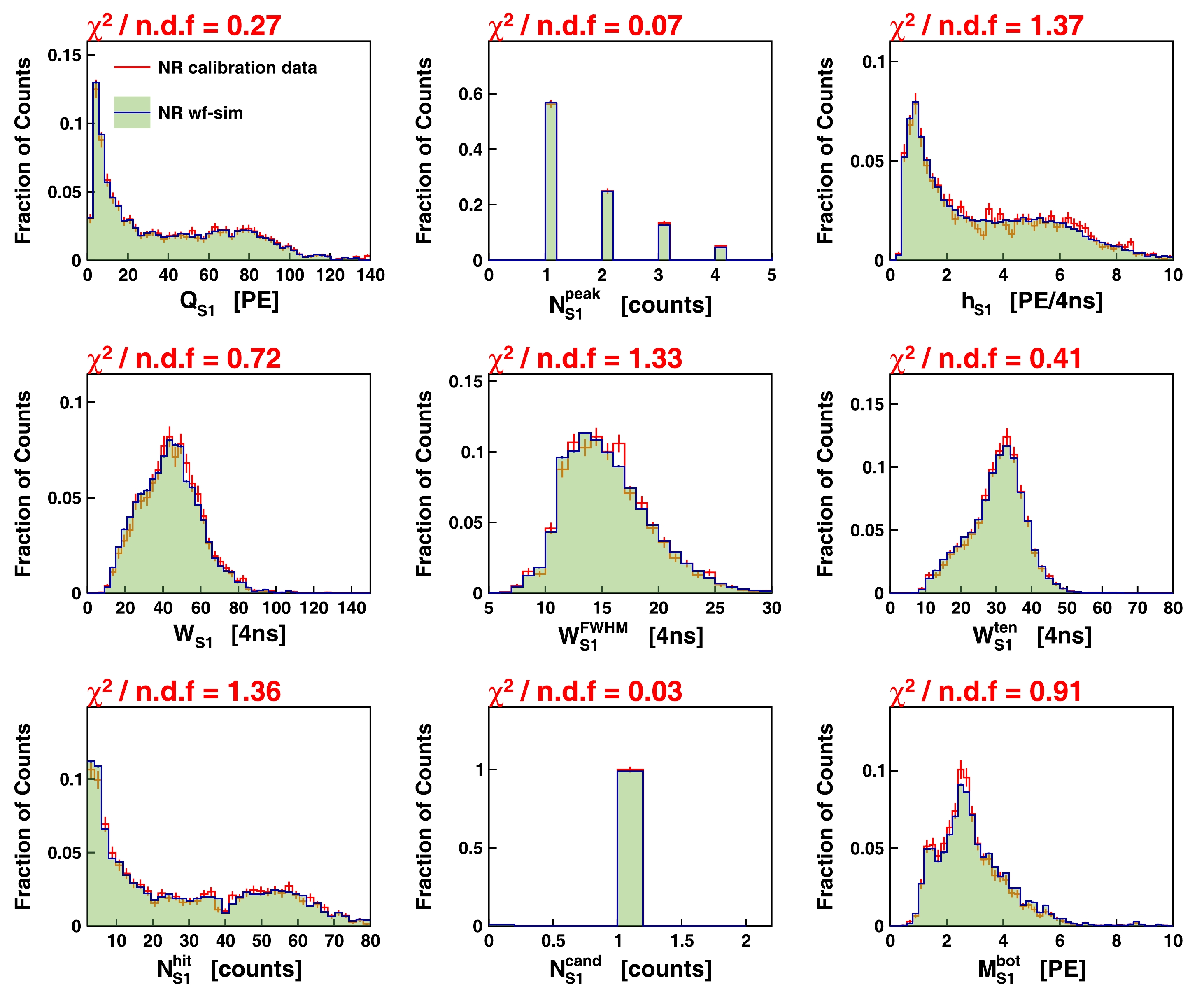
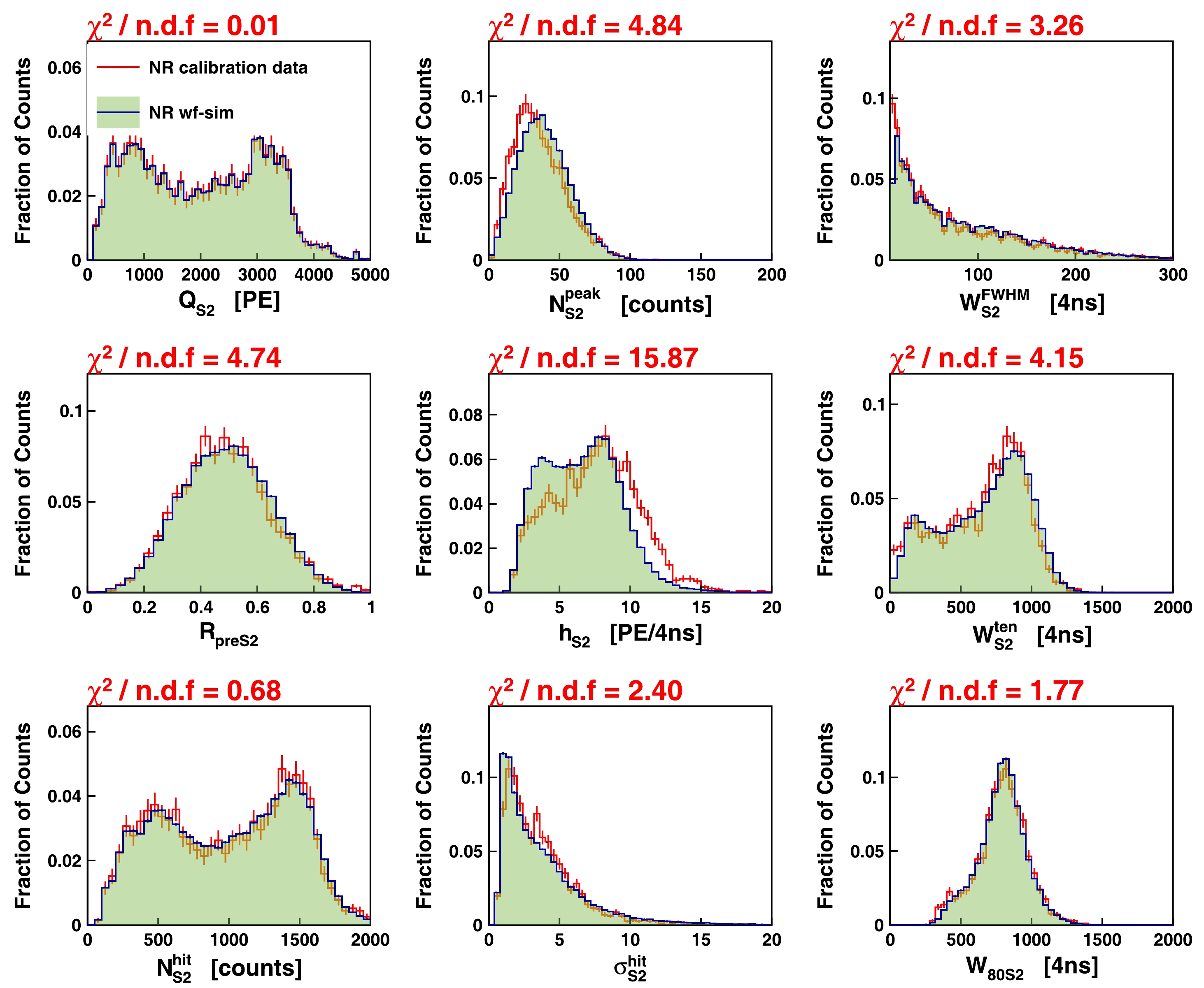
Because it is crucial to verify the fidelity of the WS by closely matching the pulse shapes of the simulated waveforms to those observed in real data, a comparison was conducted between the WS and data based on a set of selected variables, including pulse height, pulse width, number of hits, and hit charge variations. The comparisons were performed using the ER and NR calibration data, and the chi-square values were used as a measure of agreement. Figs. 10−13 illustrate the comparisons for the S1 and S2 pulses in the ER and NR calibration data. The majority of the variables demonstrated good agreement between the WS and data, with only a few variables exhibiting noticeable differences, including
$ h_{S2} $ ,$ \sigma_{S2}^{ \rm{hit}} $ , and$ N_{S2}^{ \rm{peak}} $ . This is speculated to arise from the limited statistical significance of the calibration data comprising the S1 and SE pools in the WS. In addition, a relaxed selection criterion was employed for these S1 and SE events to augment the statistics, potentially introducing impurities into the collected data.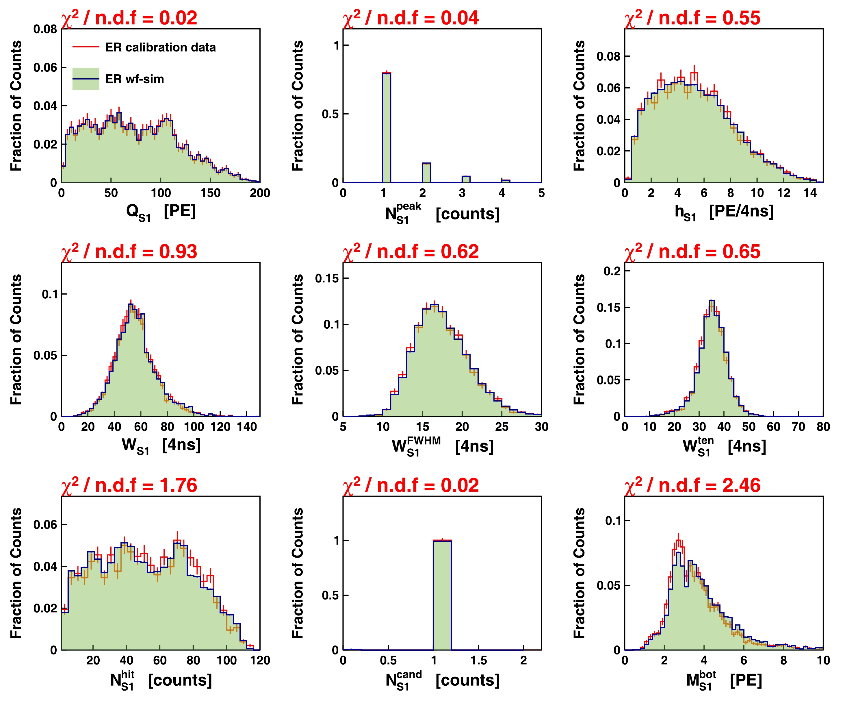
Figure 10. (color online) Comparisons of S1 key variables related to pulse shapes using ER calibration data. Red error bars represent data distribution, and shaded green histogram shows distribution from WS.
$ \chi^2 $ values divided by the degree of freedom are shown on top of each panel.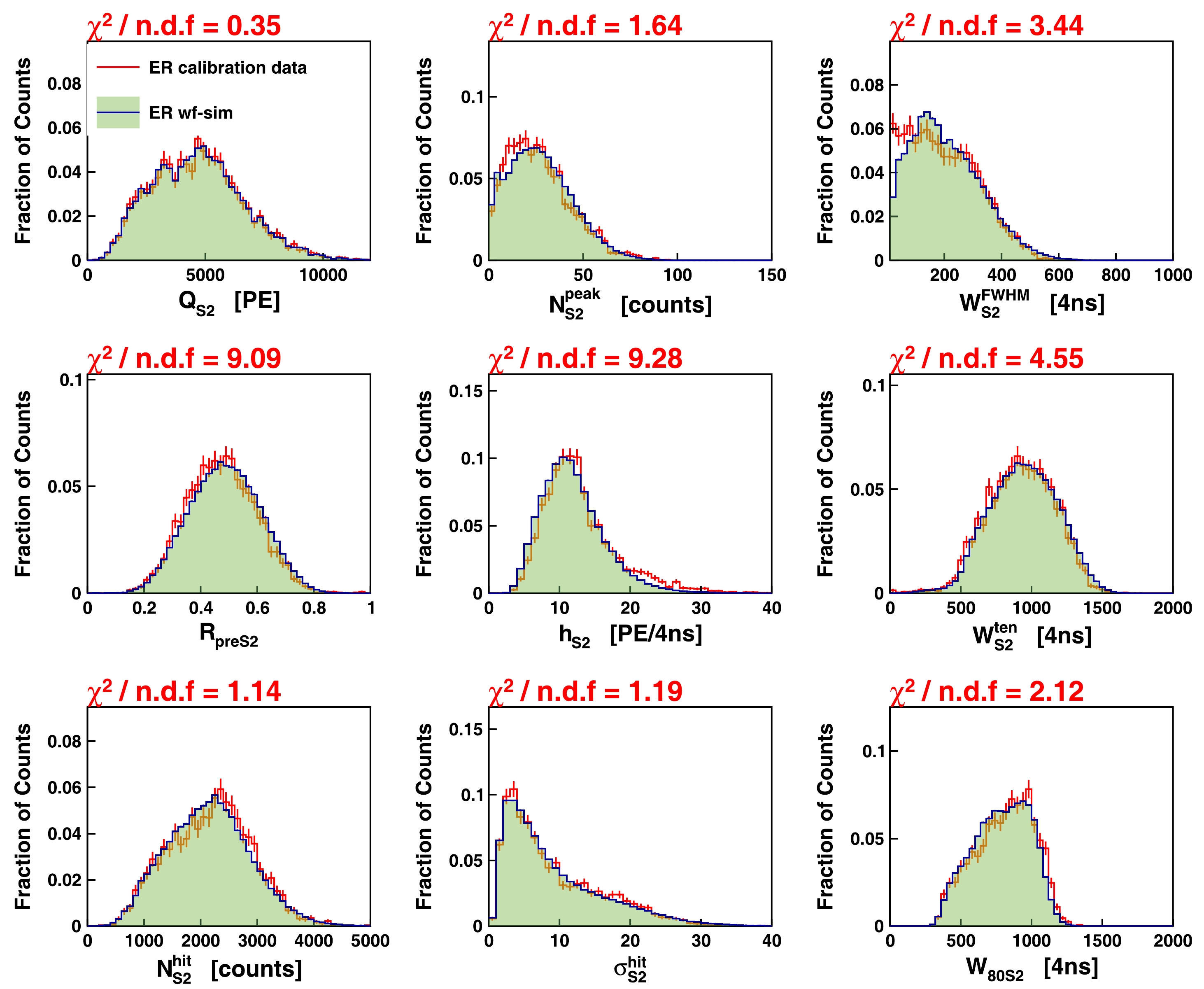
Figure 11. (color online) Comparisons of S2 key variables related to pulse shapes using ER calibration data. Red error bars represent data distribution, and shaded green histogram shows distribution from WS.
$ \chi^2 $ values divided by degree of freedom are shown on top of each panel. -
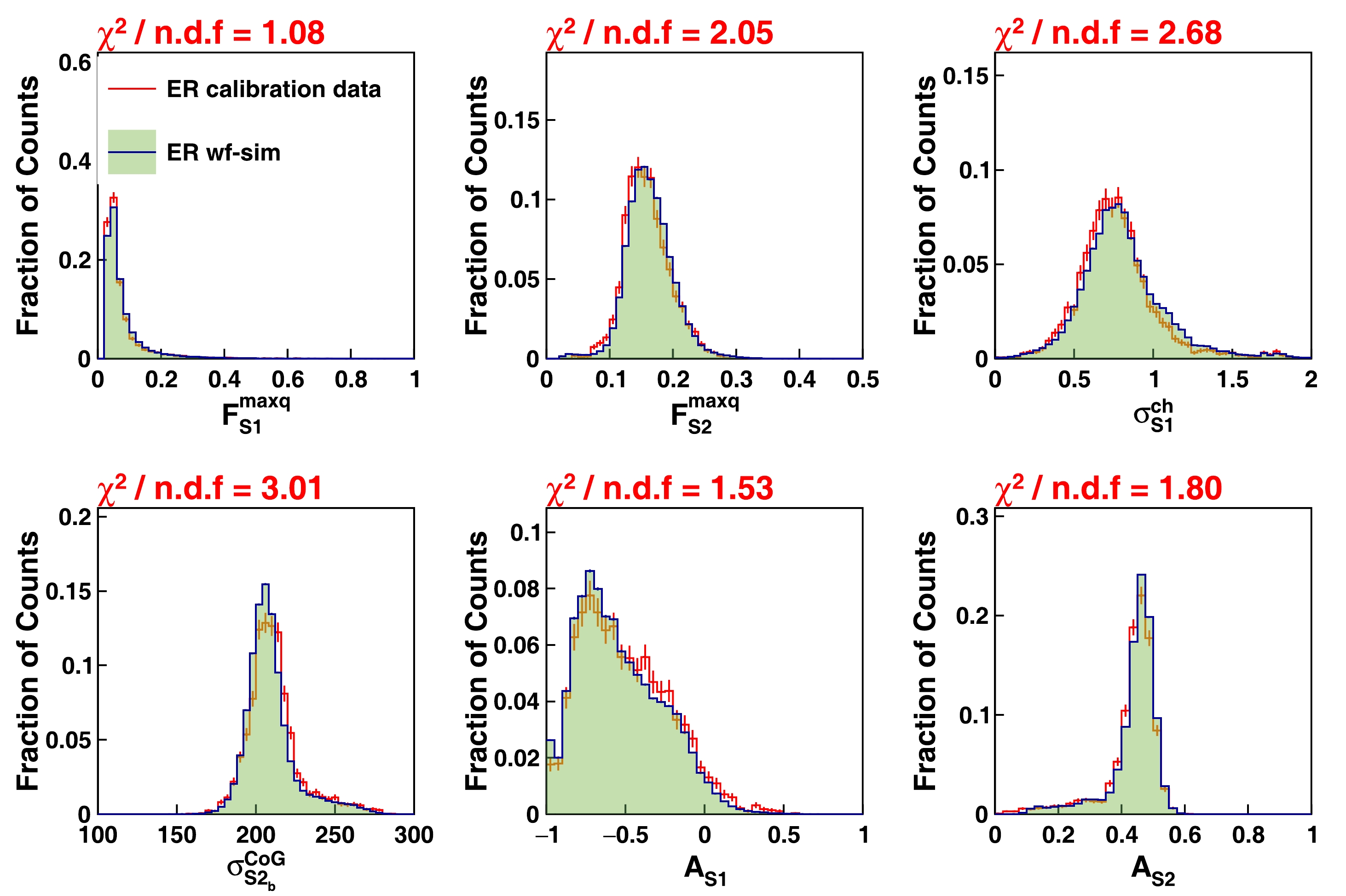
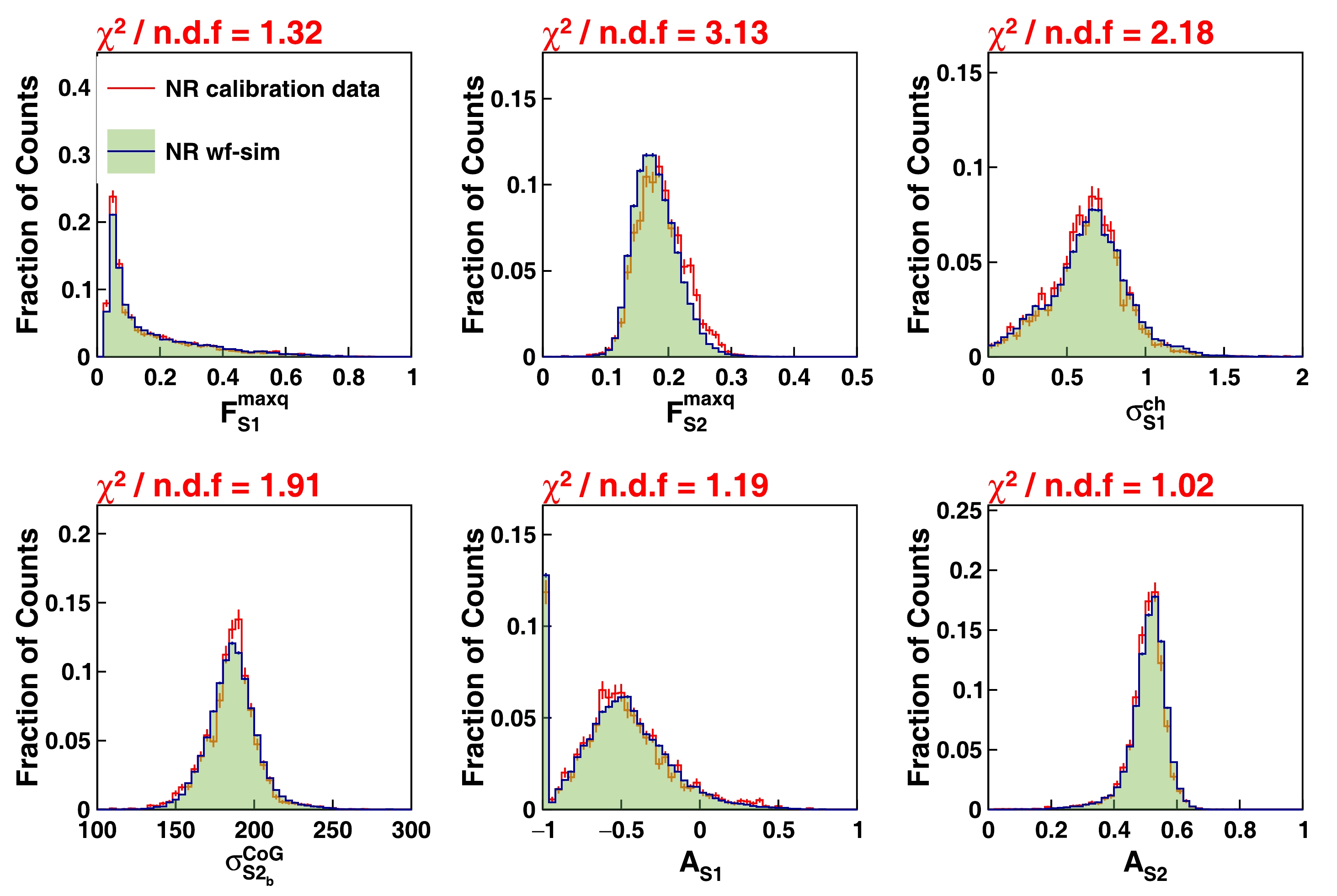
In addition to the temporal features of the simulated pulses, the pattern on the PMTs plays a crucial role. Figures 14 and 15 show the comparison of the S1 and S2 pattern related variables between the WS and calibration data, including the top-bottom asymmetries for the S1 and S2 signals, standard deviation of the hit charges among the fired PMTs, and RMS of the hit PMT positions. Most variables show good agreement, except the fraction of the S2 charge on the most-fired PMT over the total S2 charge
$ F_{S2}^{ \rm{maxq}} $ . This is attributed to the inherent uncertainty in the reconstructed positions of the SEs within the simulation pool. Notably, the reconstructed positions of the SEs exhibit considerable statistical uncertainty due to the low S2 charge, particularly in proximity to the edge of the TPC. Given that the actual positions of the SE blocks constituting the simulated S2 may not align with the expected position, discrepancies in the S2 pattern-related variables between the data and WS may arise. -
The presence of spurious noise in the waveforms can introduce incompatibility between the WS and data. To evaluate this effect, direct comparisons were performed for several selected variables, as summarized in Table 1 and depicted in Figs. 16 and 17. The initial results indicate slight deviations between the WS and data, suggesting the need for adjustments in the production probability of the photoionization model within the WS. Subsequent modifications were made based on these findings, leading to a satisfactory improvement in the matching between the WS and data.
-
We presented a detailed overview of the WS framework developed for the PandaX-4T experiment. This WS framework has been extensively utilized to address various research objectives that require a sufficient statistical sample size, which may not be readily available in the experimental data. The primary application of the WS framework is to generate synthetic samples for conducting studies related to reconstruction efficiency and bias, as referenced in [35]. Additionally, the WS framework serves as a valuable resource for generating training samples for boosted decision tree algorithms, as mentioned in [15]. Through our analysis, we demonstrated that the data-driven waveform simulation provides a comparable description of the experimental waveforms, particularly in terms of the pulse shape, pulse pattern, and presence of spurious noise. This highlights the effectiveness and reliability of the WS framework in capturing important features of the observed data. With more calibration data and understanding of the detector, we expect to further improve the WS framework, especially in terms of the correlation between the pulse shape and pattern, as well as its efficacy in high-energy regimes. Additionally, we envision broadening the application of the WS framework to encompass the interpretation of a wider range of physical models.
-
We would like to thank the sponsorship from the Chinese Academy of Sciences Center for Excellence in Particle Physics (CCEPP), Hongwen Foundation in Hong Kong, Tencent Foundation in China, and Yangyang Development Fund. We would also like to thank the CJPL administration and Yalong River Hydropower Development Company Ltd. for their indispensable logistical support and help.
Waveform simulation in PandaX-4T
- Received Date: 2023-12-18
- Available Online: 2024-07-15
Abstract: Signal reconstruction through software processing is a crucial component of the background and signal models in the PandaX-4T experiment, which is a multi-tonne dark matter direct search experiment. The accuracy of signal reconstruction is influenced by various detector artifacts, including noise, dark count of photomultiplier, photoionization of impurities in the detector, and other relevant considerations. In this study, we presented a detailed description of a semi-data-driven approach designed to simulate a signal waveform. This work provides a reliable model for the efficiency and bias of the signal reconstruction in the data analysis of PandaX-4T. By comparing critical variables that relate to the temporal shape and hit pattern of the signals, we found good agreement between the simulation and data.


 Abstract
 HTML
HTML Reference
 Related
 PDF
PDF




 DownLoad: