-
Massive stars greater than eight solar masses frequently end their lives as core-collapse supernovae (hereafter referred to as SN), but these phenomena are considerably rare and occur only approximately three times per century in our galaxy [1]. Each SN explosion ejects a significant amount of material and lasts for approximately 10 s. The total energy released by an SN burst is approximately
$ 10^{53} $ erg, with 99% carried away by neutrinos [2]. The first recorded SN neutrinos were from SN 1987A located in the Large Magellanic Cloud. Approximately 20 neutrino events were detected [3−5], marking the beginning of the galactic neutrino astronomy. These neutrino events provide significant insights into the theoretical models of SN explosions and offer constraints to the fundamental properties of neutrinos. However, our present understanding remains inadequate for a thorough comprehension of stellar dynamics and neutrino properties at extreme conditions owing to the low statistics of the observed SN neutrino events. Many neutrino experiments and observatories have been designed with full readiness to observe imminent SN explosions.During an SN explosion, numerous neutrinos are emitted from the central region of the star at nearly the speed of light. In contrast, electromagnetic radiation experiences a delayed travel compared with the neutrinos owing to the smaller velocity of outward shock waves [6]. The delay may vary from several minutes to several days depending on the SN progenitors. Neutrino observatories located on the Earth can utilize the abrupt increase in the neutrino event rate to provide a prompt alert of the occurrence of an SN explosion in our galaxy to trigger followup optical observations. To date, several experiments have established dedicated SN monitoring systems [6−8] and initiated joint observations with the SN early warning system (SNEWS) [9, 10].
Freedman indicated that coherent elastic neutrino-nucleus scattering (CEνNS) can occur when the incident neutrino energy is on the order of MeV [11]. This implies a large cross section,
$ \sigma_{\nu}\simeq N^{2}G^{2}_{F}E^{2}_{\nu}/4\pi $ , where N represents the neutron number of the target nuclei,$ G_F $ is the Fermi constant, and$ E_{\nu} $ is the neutrino energy [12]. Such a process has been observed in the COHERENT experiment with neutrinos from the spallation neutron sources with an average energy about 30 MeV, providing a sensitive tests on the Standard Model of particle physics [13]. Hence, direct detection dark matter experiments using liquid xenon (LXe), for example, the operating XENONnT/LUX-ZEPLIN/PandaX-4T experiments [14−16] and the proposed DARWIN [17] and PandaX-xT experiment [18], are appropriate options for detecting SN neutrinos owing to the large neutron number of the nucleus of about 80. As the fiducial mass of these experiments increase to above a ton and even ten-ton level, the CEνNS process demonstrates the increasing competitiveness in the detection of astrophysical neutrinos compared with other neutrino interaction channels. The CEνNS process is sensitive to all neutrino flavors equally, thereby complementing the studies of experiments that have particular sensitivity to an individual neutrino flavor [19, 20]. A prominent challenge is that the momentum transfer of the process is very small, resulting in low nuclear recoil (NR) energy in the order of keV, which is difficult to detect. Thus far, no experiment has observed astrophysical neutrinos via the CEνNS process.In this paper, the SN model from the Garching group (hereafter referred to as Garching model) is utilized to obtain the neutrino emission spectrum of an SN explosion [21, 22]. For comparison, a model proposed by Nakazato et al. is also discussed [23]. We do not consider neutrino oscillations as we are solely focusing on the overall neutrino flux. By considering the neutrino flux, cross section, exposure, and detection efficiency, the total number of expected neutrinos in PandaX-4T is obtained. A method for accurately predicting the false alert rate is developed. Based on this framework, two specialized triggering alarms, golden and silver, for monitoring SN burst neutrinos are introduced, which can be easily implemented at the software level. Furthermore, the probability of detecting SN explosions in our galaxy out to 50 kpc is estimated. In addition, with the commissioning data acquired from PandaX-4T, an upper limit for the occurrence of SN explosions in the Milky Way is extracted.
The remainder of this paper is organized as follows. The PandaX-4T experimental setup and data processing are described in Sec. II. The detection of SN neutrinos at PandaX-4T is presented in Sec. III. The trigger algorithm is discussed in Sec. IV. The detection probability and the upper limit of SN bursts are described in Sec. V. The conclusions are contained in Sec. VI.
-
The PandaX-4T experiment at China Jinping Underground Laboratory (CJPL) has been on operation since November 2020. The cosmic-ray muons are effectively shielded by a rock overburden of approximately 2,400 m. The detector is located within an ultra-pure water shield measuring 13 m in height and 5 m in radius. This configuration reduces the impact of the radioactivity that originates from the ambient environment. The detector is a dual-phase xenon time projection chamber (TPC) with about 3.7-t of LXe in the sensitive volume and 368 Hamamatsu R11410-23 3-inch photo-multipliers (PMTs) that are arranged in a concentric circular (compact hexagonal) for top (bottom) array. The peripheral background is vetoed by an outer array of 105 Hamamatsu R8520 1-inch PMTs. An upward drift and acceleration electric field for electrons are provided by the three of four transparent stainless steel electrodes. More details are available in [24].
When incident particles pass through LXe, they can generate excited xenon atoms and electron-ion pairs. These particles are detected through the coincidence observation of photon signals from the prompt scintillation (S1) and the delayed electro-luminescence (S2). The photo-electron (PE) signals are digitized by a CAEN V1725B digitizer, which operates at a sampling rate of 250 MHz. The digitizer operates in the self-trigger mode, in which any PMT pulse exceeding the threshold of 1/3 PE is recorded. The data are transferred to multiple readout servers and then to a dedicated data-aggregation server in Jingping for further processing and writing to disks. The Data are then transferred to servers located in Chengdu for offline physical analysis [25]. The commissioning data from November 28, 2020 to April 16, 2021 with a calendar time of
$ \sim $ 86 days are utilized in this study. Detailed operation conditions of the detector and event reconstructions are discussed in [16]. -
The CEνNS process can be expressed as
$ \begin{array}{*{20}{l}} \nu/\bar{\nu} + A \to \nu/\bar{\nu} + A, \end{array} $

(1) where
$ \nu/\bar{\nu} $ is any individual flavor of neutrinos/antineutrinos, and A represents the mass number of the target nuclei. The NR energy spans from zero to a maximum value of$E_{\max} = 2E^{2}_{\nu}/(2 E_{\nu} + m_{A}) \simeq 2E^{2}_{\nu}/m_{A}$ , where$ m_{A} $ is the mass of the target nucleus. The differential cross section of the CEνNS process can be expressed as [11, 12]$ \begin{split} \frac{{\rm d}\sigma}{{\rm d}E_{\rm NR}}(E_{\nu},E_{\rm NR}) =\; &\frac{G^{2}_{F}m_{A}}{4\pi} Q^{2}_{w} \left(1-\frac{m_{A}E_{\rm NR}}{2E^{2}_{\nu}}\right) \\ &\times F^{2}(q)\Theta(E_{\max}-E_{\rm NR}), \end{split} $

(2) where
${E_{\rm NR}}$ represents the NR energy of the target nucleus,$\Theta(E_{\max}-E_{\rm NR})$ is the step function with a value of 1 (0) for positive (negative) argument, and$ Q_{w} $ is the weak charge:$ \begin{array}{*{20}{l}} Q_{w} = N - Z(1-4\text{sin}^{2}\theta_{w}), \end{array} $

(3) where Z is the atomic number of the target nucleus,
$ \theta_{w} $ is the weak mixing or Weinberg angle with a value of${\rm sin}^{2}\theta_{w} \simeq 0.23$ [26], and$ F(q) $ is the Helm-type form factor [27], which is defined as$ F(q) = \frac{3j_{1}(qr_{0})}{qr_{0}}{\rm e}^{-\frac{1}{2}(qs)^{2}}, $

(4) where the momentum-transfer
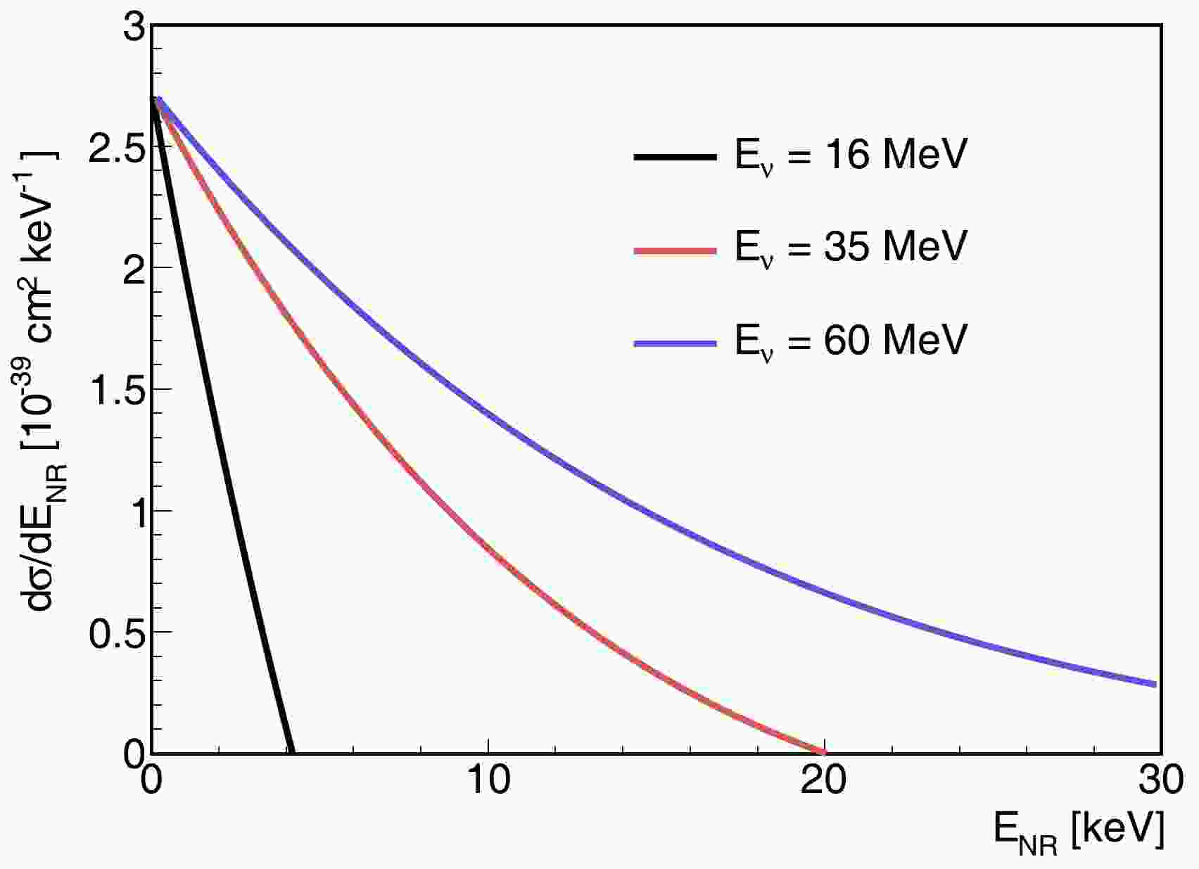
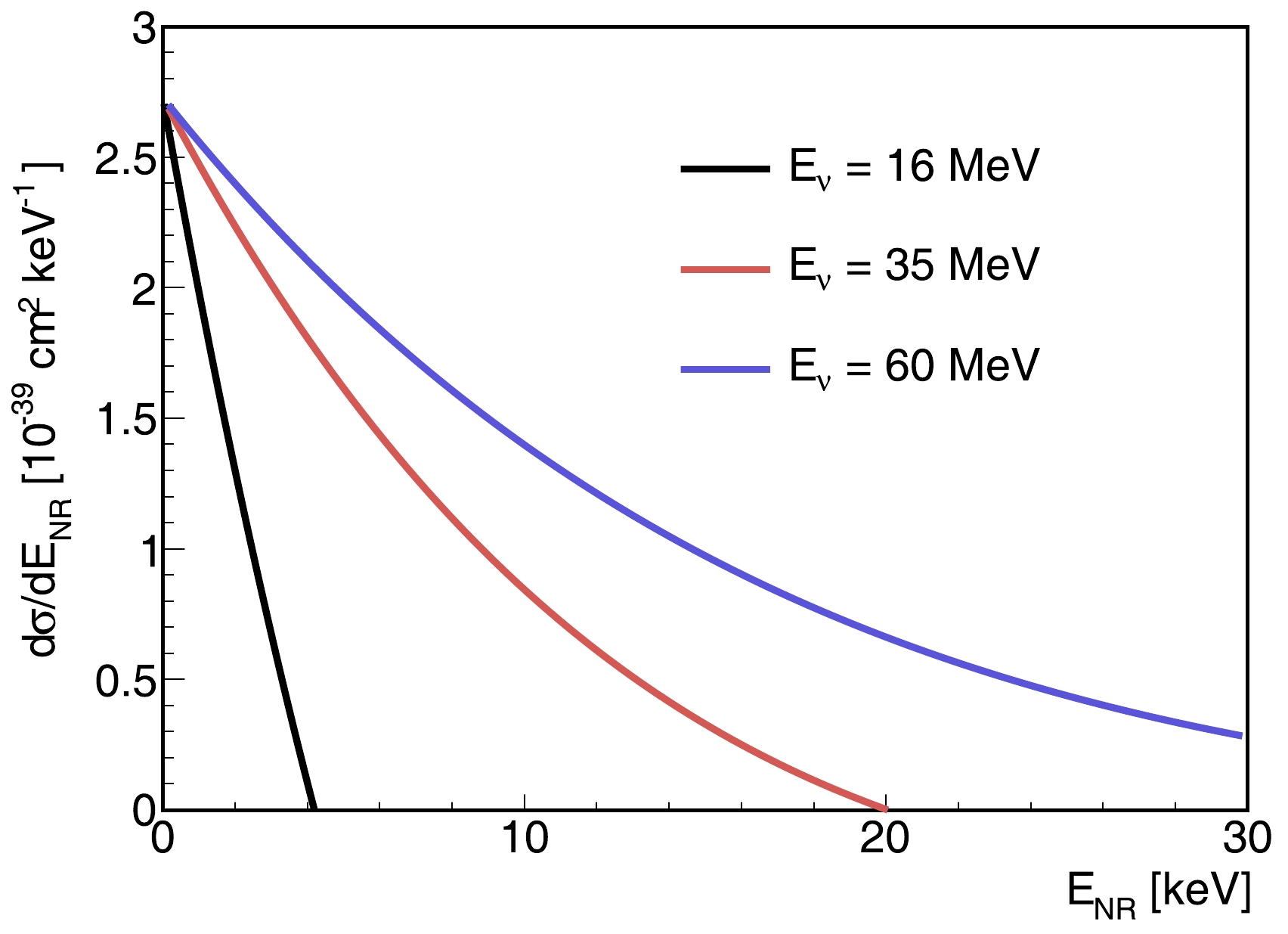
$ q=\sqrt{2m_{A}E_{N R}} $ ,$r_{0}= \sqrt{r^2 - 5s^2}$ with a nuclear radius of$ r=1.2A^{\frac{1}{3}} $ fm and nuclear skin thickness s of about 0.5 fm, and$ j_{1}(qr_{0}) $ is the first-order spherical Bessel function [28, 29]. Figure 1 shows the differential cross section of Eq. (2) at different neutrino energies. Note that the CEνNS exhibits a much larger scattering cross section [12] than inverse beta decays and neutrino-electron elastic scatterings [13] but results in a relatively low NR energy in keV to several tens of keV. The abundance distribution of xenon isotopes is considered in the calculation. -
The SN explosion consists of three stages: the phase of the shock burst, the post-bounce accretion, and Kelvin-Helmholtz cooling [21]. The total emission energy, average energy of neutrinos, and variations in the physical process will lead to different expected fluxes and energy spectra of neutrinos in theoretical models. In this study, we utilize the Garching model as the typical model, where the neutrino energy spectrum can be characterized using Keil-Raffelt-Janka (KRJ) parametrization [30]. The differential flux at time
$ t_\mathrm{pb} $ , which is defined as the time after the SN core bounce, can be expressed as [31, 32]$ \begin{split} \frac{{\rm d}F(E_{\nu},t_\mathrm{pb})}{{\rm d}E_{\nu}} =\; &\sum\limits_{\nu = 1}^{6} L_{\nu}(t_\mathrm{pb}) \frac{ ( 1+\gamma (t_\mathrm{pb}) ) ^{1+\gamma (t_\mathrm{pb}) }}{\langle E_{\nu}(t_\mathrm{pb}) \rangle ^{2} \Gamma (1+\gamma (t_\mathrm{pb}) )} \\ & \times \left(\frac{E_{\nu}}{\langle E_{\nu} (t_\mathrm{pb}) \rangle } \right) ^{\gamma(t_\mathrm{pb})} \exp\left[-\frac{(\gamma + 1)E_{\nu}}{ \langle E_{\nu} (t_\mathrm{pb}) \rangle } \right] , \end{split} $

(5) where ν represents one of the six types of neutrinos,
$ L_{\nu}(t_\mathrm{pb}) $ is the neutrino luminosity,$ \langle E_{\nu}(t_\mathrm{pb}) \rangle $ is the mean energy of neutrinos at time$ t_\mathrm{pb} $ , and$ \Gamma(1+\gamma (t_\mathrm{pb})) $ is the Gamma function. The spectral index$ \gamma(t_\mathrm{pb}) $ can be obtained as [31]$ \frac{\langle E_{\nu}(t_\mathrm{pb}) ^{2} \rangle}{\langle E_{\nu}(t_\mathrm{pb}) \rangle ^{2}} = \frac{2 + \gamma (t_\mathrm{pb}) }{1+ \gamma (t_\mathrm{pb})}, $

(6) where
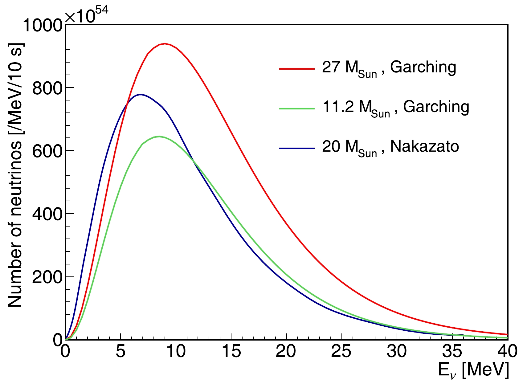
$ \langle E_{\nu}(t_\mathrm{pb}) ^{2} \rangle $ represents the mean of$ E_{\nu}(t_\mathrm{pb}) ^{2} $ . Here, we use models with two benchmark progenitor masses$ M_{p}=11.2\; M_{\odot} $ and$ M_{p}=27\; M_{\odot} $ ($ M_{\odot} $ is the solar mass), employing the LS220 nuclear equation of state (EoS) [33], to predict the neutrino fluxes and the energy spectra. In contrast, the Nakazato model with$ M_{p}=20\; M_{\odot} $ , metallicity Z=0.02, and shock revival time$t_{\rm rev}=200$ ms is also used [23]. Figure 2 depicts the time-integrated neutrino number spectrum of all types of neutrinos. For a clear visual comparison between the models, neutrino energies are shown only up to 40 MeV. Because the neutrino flux from an SN explosion is predominantly concentrated within the first few seconds after the core bounce, we have approximated the integration time for the Nakazato model to be 10 s. The fraction of neutrino flux beyond 10 s is negligible. For the Garching models, we integrate from the core bounce time to the end time of the models since the models do not extend to 10 s. -
When neutrinos interact with xenon atoms through the CEνNS process, the differential event rate can be described as
$ \begin{split} \frac{{\rm d}N_{0}}{{\rm d}E_{\rm NR}}(E_{\rm NR})=\;&\frac{m_{\rm det}N_{A}}{M_{A}(4\pi D^{2})} \int_{E^{\min}_{\nu}}^{\infty} \frac{{\rm d}\sigma}{{\rm d}E_{\rm NR}}(E_{\nu},E_{\rm NR}) \\ &\times f(E_{\nu}){\rm d}E_{\nu}, \end{split} $

(7) where
$m_{\rm det}=2.67$ t is the effective mass of LXe in this paper,$ N_{A} $ is Avogadro's constant,$ M_{A} $ is the molar mass of xenon atoms, and the expression$m_{\rm det} N_{A}/ M_{A}$ is the total number of xenon atoms in the detector. D is the distance from Earth to the SN. To produce a recoil energy above$E_{\rm NR}$ , we must have a minimum neutrino energy, which can be expressed as$E^{\min}_{\nu} = \sqrt{m_{A} E_{\rm NR}/2}$ and is the lower limit of the integral in Eq. (7).$ f(E_{\nu}) $ is the energy spectrum for the sum of all neutrino types, as depicted in Fig. 2. Practically, integrating over$E_{\nu} \in (E^{\min}_{\nu},100$ MeV) is sufficient. Considering the detection efficiency$\epsilon(E_{\rm NR})$ , the effective differential event rate is [34]$ \frac{{\rm d}N}{{\rm d}E_{\rm NR}}(E_{\rm NR})= \epsilon (E_{\rm NR}) \times \frac{{\rm d}N_{0}}{{\rm d}E_{\rm NR}}(E_{\rm NR}). $

(8) To obtain the detection efficiency, we perform a Monte Carlo (MC) simulation [35, 36]. First, the light yield (
$ L_{y} $ ) and charge yield ($ Q_{y} $ ) of NR events in LXe are studied using the Noble Element Simulation Technique (NEST) v2.3.6 parameterization [37, 38], with parameters tuned using the calibrations as described in [16, 39]. In the simulation, we have considered various detector effects, including the quantum effects of PMTs and the non-uniformity of the detector.$ 2 \times 10^{5} $ events are simulated for each mono-energetic point ranging from 0.1 to 30 keV, with a step size of 0.1 keV. Subsequently,$ L_{y} $ and$ Q_{y} $ are used as the inputs for the waveform simulation (WS) [36], which can generate complete waveforms. To mimic the detector response of the simulated events, we consider the effects of afterpulsing from PMTs and delayed electrons in the WS process.The simulated events are processed with similar procedures as in the experimental data. The total efficiency primarily consists of three parts: the signal reconstruction, data quality selection, and region-of-interest (ROI). The signal reconstruction and data quality selection were discussed in detail in a previous analysis [39]. To improve the detection efficiency, we loosen several data quality selection cuts and adjust the ROI. Two ROIs are used: one corresponds to the golden alert, which is stricter in triggering SN alarms than the silver one. The former (latter) is defined to have S1 ranging from 2.1 to 100 PEs (1.65 to 100 PEs) and S2 ranging from 80 to 3500 PEs (same). This is detailed in Sec. IV. The magenta dashed (red solid) line depicted in Fig. 3 shows the detection efficiency as a function of NR energy for the golden (silver) alarm. A decrease in efficiency occurs at energies above 15 keV, which is attributed to the diffusion cut on the drift electrons in the selection process. The total detection efficiency is 20% (23%) for the golden (silver) alarm in the Garching model with
$ M_{p}=27\; M_{\odot} $ , and other two SN models used in this paper have similar efficiencies. Note that, to maximize the detection efficiency, this study does not use the NR/ER cut based on the ratio between the number of the ionized electrons and the photons. Additionally, this can be revived in the PandaX-nT experiment owing to the much larger target mass.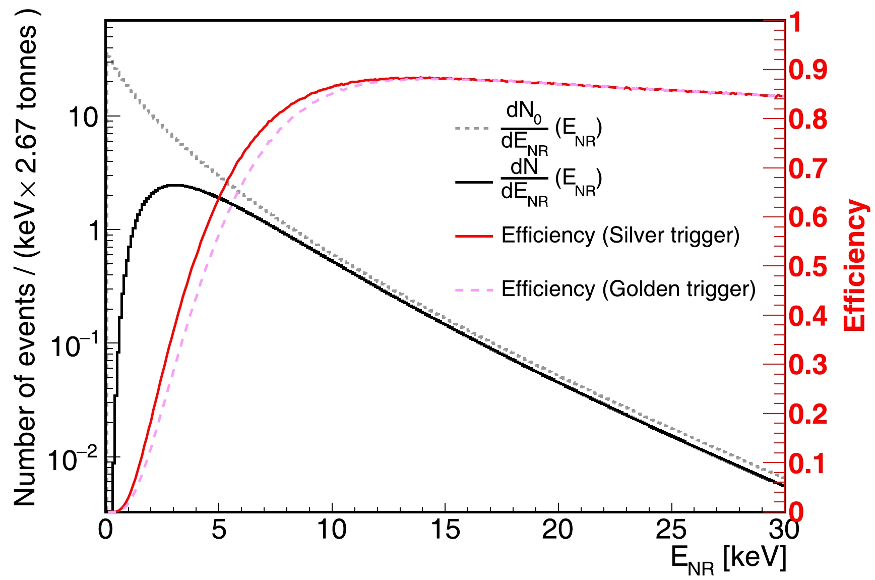
Figure 3. (color online) Detection efficiencies of silver trigger (red solid) and golden trigger (magenta dashed) as a function of NR energy; the expected neutrino spectrum before (gray) and after (black) the efficiency (red solid) correction. The Garching model with a progenitor mass of
$ 27\; M_{\odot} $ and the LS220 EoS is used. The distance from SN to Earth is assumed to be 10 kpc.The NR spectrum of CEνNS before (gray) and after (black) the efficiency (red solid) correction in LXe is shown in Fig. 3. The total expected number of observable neutrinos
$N_{\rm obs}$ , which is primarily from the high-energy neutrinos (approximately 15 to 30 MeV), as shown in Fig. 2, can be expressed as$ N_{\rm obs}= \int \frac{{\rm d}N}{{\rm d}E_{\rm NR}}(E_{\rm NR}) {\rm d} E_{\rm NR}, $

(9) here, we perform the integration up to 30 keV because fluxes above this value have a negligible impact on
$N_{\rm obs}$ . To increase$N_{\rm obs}$ , we desire a high detection efficiency. The numbers of SN neutrinos using the Garching and Nakazato models at two different distances of 10 kpc and 168 pc are listed in Table 1, where 10 kpc (168 pc) is approximately the distance from the center of the Milky Way (Betelgeuse) to Earth. Ref. [31] shows that an S2 only method can increase the SN signals by a factor of about 3 but would also potentially increase the backgrounds. The S1-S2 method provides similar results as ours. The background event rate, as listed in Table 2, is negligible compared with the event rate of the SN signals as listed in Table 1. Betelgeuse is considered a potential candidate for an SN explosion [40], which would provide an effective handle to distinguish between different models by observing the number and spectrum of NR events owing to the short distance. For a Betelgeuse explosion, the design of the data acquisition must address the challenge of high data rate during the explosion.SN model Golden alarm Silver alarm D = 10 kpc 168 pc 10 kpc 168 pc 20 $ M_{\odot} $ Nakazato

7.2 $2.6 \times 10^{4} $ 

8.3 $ 2.9\times 10^{4} $ 

11.2 $ M_{\odot} $ Garching

6.6 $2.3 \times 10^{4} $ 

7.7 $2.7 \times 10^{4} $ 

27 $ M_{\odot} $ Garching

13.7 $4.9 \times 10^{4} $ 

15.9 $5.7 \times 10^{4} $ 

Table 1. Number of expected SN neutrinos from 10 kpc and 168 pc in PandaX-4T for golden and silver alarms. Two Garching models are used with
$ M_{p}=11.2\; M_{\odot} $ and$ M_{p}=27\; M_{\odot} $ via the LS220 EoS. Nakazato model with$ M_{p}=20\; M_{\odot} $ , Z (metallicity)$ =0.02 $ , and$t_{\rm rev}$ (the shock revival time)$ =200 $ ms is used for comparison.Data type Rate/s Calendar time Observed Expected DD 3.61× $ 10^{-3} $ 

3.58 days 40 38 AmBe 3.12× $ 10^{-3} $ 

5.7 days 49 46 Physical 3.6× $ 10^{-4} $ 

86.1 days 8 9.8 Table 2. Comparison of the observed and expected false alerts with the silver trigger mode using the DD, AmBe, and physical data as listed in the fourth and fifth columns. The second and third columns list the event rate and the calendar time of the dataset.
-
The explosion of an SN would result in a sudden increase in the event rate within a short period of several seconds in the detector, providing a unique opportunity to observe this phenomenon in the Milky Way. The software-based SN trigger can provide a method for monitoring SN explosions as soon as data files are written into the disk clusters. The trigger algorithm consists of three parts: 1) event builder, 2) selection of signal candidates, and 3) SN neutrino trigger. The event builder process involves clustering PMT hits into signal pulses and classifying these pulses into S1s and S2s, where the classified S1s and S2s are paired to build incident events. The size of each file decreases significantly after the event builder process, from 1 GB to approximately 100 MB. During the commissioning phase, the background event rate is stable. To select suitable event candidates, the basic cuts derived from the analysis of the solar
$ ^8 $ B study [39] are used to suppress background events. The events that survive the cuts are used to investigate the false alert rate, which is discussed in Sec. IV.B. For the SN neutrino trigger, when the trigger algorithm identifies the first candidate, it serves as the starting point of the search time. Subsequently, the total number of events is counted within the following ten-second time window. If the counted number exceeds the specific threshold$N_{\rm thr}$ , a prompt alert is issued. For clarity, if another candidate appears outside of the time window, it will become a new starting point of the search time, and the same process continues. When an alert is issued, the information including the start time of the alert and the total number of candidates in the time window are sent simultaneously to the experts of the PandaX-4T SN group through e-mail. The relevant data files are stored in the designated directory for further examination by the experts. The entire process takes several minutes for each individual file on average. -
We assume that the number of events observed by the detector follows a Poisson distribution. The probability for the number of events in a time window
$T_{\rm SN}$ being no less than the threshold value$N_{\rm thr}$ follows$ p(N_{\rm thr};T_{\rm SN};r_{\rm bg}) = 1 - \sum\limits_{n=0}^{N_{\rm thr} -1} \frac{1}{n!} {\rm e}^{-r_{\rm bg}T_{\rm SN}} (r_{\rm bg}T_{\rm SN})^{n}, $

(10) where
$r_{\rm bg}$ is the mean background event rate. The false alert rate per week using a fixed time window$T_{\rm SN}$ can be expressed as$ R_{\rm false} = \frac{3600 \cdot 24 \cdot 7 }{T_{\rm SN}} p(N_{\rm thr};T_{\rm SN};r_{\rm bg}). $

(11) The backgrounds are primarily composed of material radioactivity, environmental radioactivity, contamination from tritium calibration, and additional radioactive sources in xenon such as
$ ^{222} $ Rn [24]. To improve the SN detection probability while simultaneously reducing the false alert rate, we investigate various combinations of$T_{\rm SN}$ and$N_{\rm thr}$ at a certain event rate$r_{\rm bg}$ . Eventually, a suitable combination of the values is selected, with$T_{\rm SN}=10$ s and$N_{\rm thr} =2$ . Unless stated otherwise, we will use this default setting. The false alert rate is predicted with a two-step procedure. In the first step, we can calculate the number of false alert rate for a given event rate$r_{\rm bg}$ and time window using Eq. (11). Note this number is for the case of the fixed time window (i.e., the subsequent time window is seamlessly connected to the previous time window; therefore, no time gap occurs between any two time windows), and in our algorithm, we use the sliding time window (i.e., the time of the candidate is used as the start of the time window, and a time gap may occur between two neighbour time windows). A schematic of sliding and fixed time window is shown in Fig. 4. In the second step, the ratio between the numbers of false alerts with the sliding and fixed time windows is calculated based on a toy MC simulation. Hereafter, the former (latter) is referred to as the SW (FW) method. In the toy MC simulation, events are randomly sampled assuming a specific event rate, followed by the counting of the total number of false alerts with the SW and FW methods. To reduce the uncertainty of the mean ratio value, hundreds of simulations are performed for each event rate. Figure 5 shows the ratio as a function of the event rate.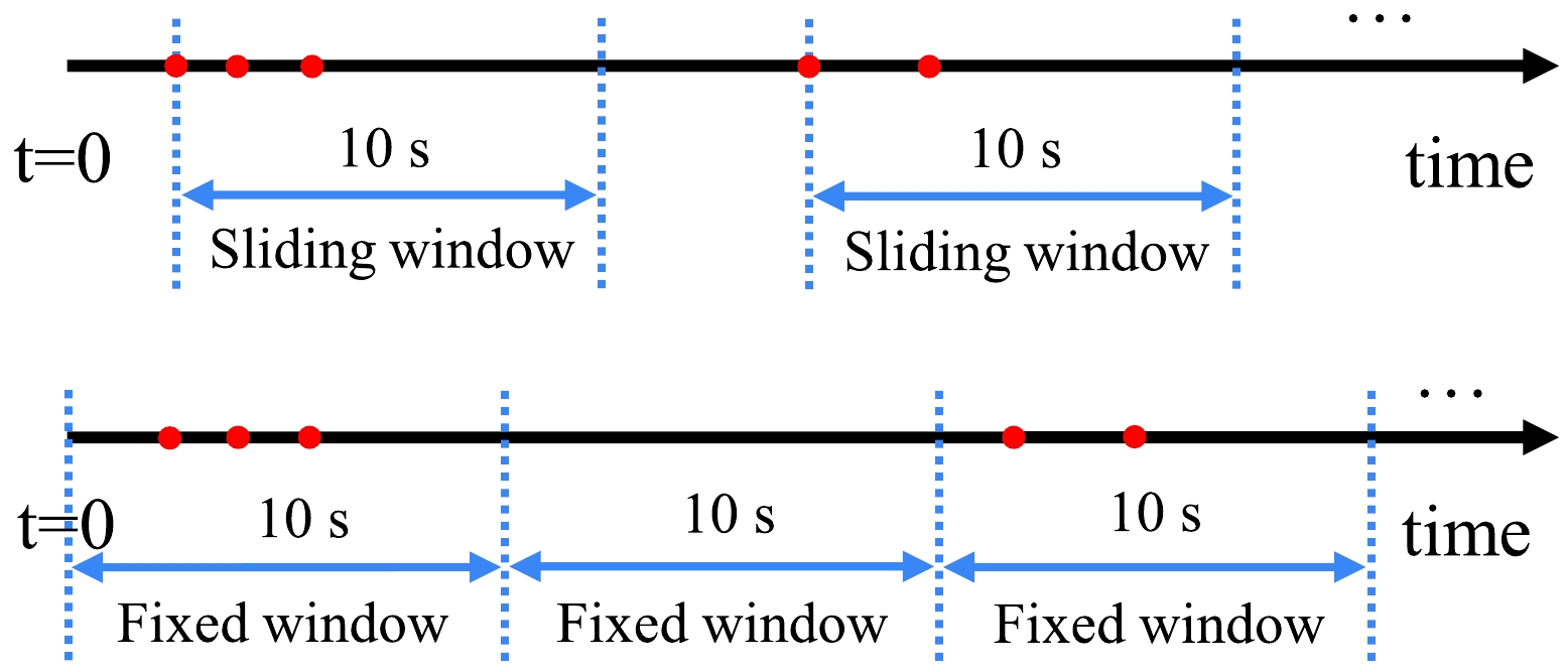
Figure 4. (color online) Schematic of the sliding and fixed time windows. The red dots represent SN neutrino candidates.
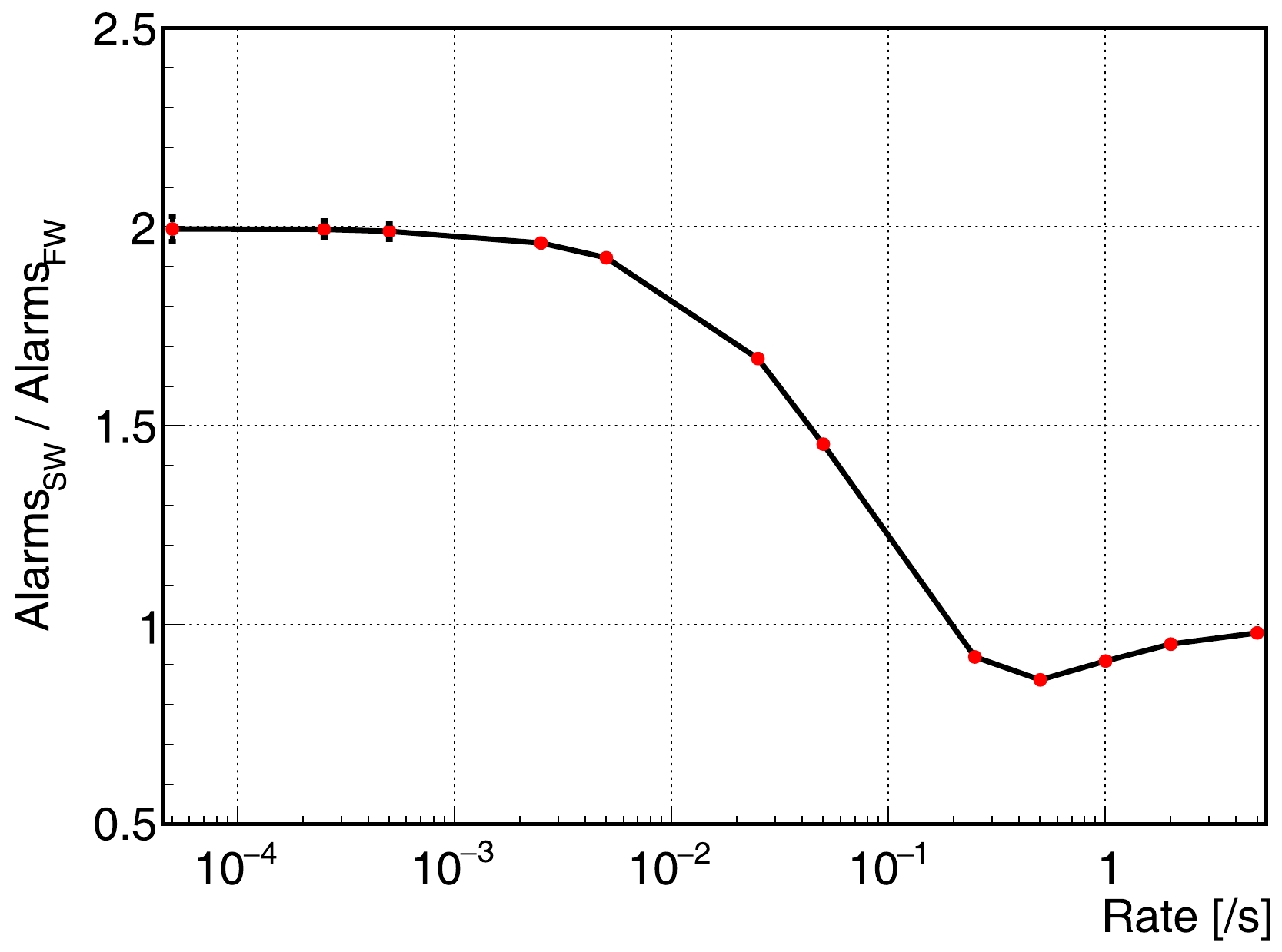
Figure 5. (color online) Ratio of the false alerts using sliding and fixed time windows. The parameters used are
$T_{\rm SN} =10$ s,$N_{\rm thr} =2$ , and the uncertainty results from the estimation of the mean values. The curve is connected through the data points via the linear interpolation, and the data points are calculated from the toy MC simulations.We must emphasize three characteristics in Fig. 5. First, when the rate is lower than
$ 10^{-3} $ s-1, the ratio gradually converges to 2. A mathematical explanation can be provided based on the the settings for this study. At the low rate, each alert comprises only two candidates with the parameters of$T_{\rm SN}=10$ s and$N_{\rm thr} =2$ ; this is because the probability of greater than two candidates appearing within 10 s is significantly lower than that of exact two candidates. If two candidates occur within a 10-s window in a total time length that can be divided into N intervals, with each interval being 5 s and N being sufficiently large, there are 3N/2 and N/2 scenarios for two candidates occurring in different intervals for the SW and FW methods, respectively, whereas the number of the scenarios for two candidates occurring in same intervals is N/2. Therefore, the ratio is$(3N/2+N/2)/ (N/2+N/2)=2$ . A ratio of 2 can also be explained as ($ r_{\rm bg}\times10 $ s)/($ r_{\rm bg}\times5 $ s) because the first candidate appears at the start (middle on average) of a 10-s window for the SW (FW) method. Note that the number of false alerts expected from Eq. (11) agrees with the number counted from the toy MC simulation using the FW method. In contrast to the SW method, the FW method divides the time length into uniform intervals according to the time window$ T_{\rm SN} $ and counts the false alerts within each interval. Second, the ratio reduces to a value below 1 because, with a higher rate, the possibility of more than two CEνNS events piling up in a single sliding window increases, leading to fewer triggers. Third, the ratio converges to 1 at a high event rate greater than 5 s-1 as the two methods exhibit negligible differences in these cases. -
To validate the false alert rate described above, we have used experimental data including the deuteron-deuteron (DD), AmBe neutron calibration, and commissioning physical data to test the trigger algorithm. Eq. (11) enables the inverse calculation of the corresponding background event rate for a given false alert rate. As stated in Sec. III.C, two trigger modes (golden and silver) for the commissioning physical data have been selected, which correspond to false alert rates (background event rates) of one per month (
$ \sim2.2\times10^{-4} $ s-1) and one per week ($ \sim3.6\times10^{-4} $ s-1), respectively. The ROI is essential in regulating the false alert rate, which is used as a reference to rapidly adjust the ROI in the commissioning physical data. The numbers of the expected false alerts are consistent with the observed, as listed in Table 2. For simplicity, only the results with silver trigger mode are shown. The scenario in which the two candidates fall into two separate files has been considered. -
The detection probability of the SN explosions is same as that in Eq. (10), with the change of
$r_{\rm bg}$ to$r_{\rm SN}$ , where$r_{\rm SN}$ is the event rate of SN neutrinos. Figure 6 shows the probability of detecting SN explosions at different distances in the golden and silver trigger modes with the Garching model, assuming a progenitor mass of$ M_{p}=27\; M_{\odot} $ . The PandaX-4T detector would have a 100% probability of detecting SN explosions in the golden and silver trigger modes assuming the SN is located 10 kpc from Earth.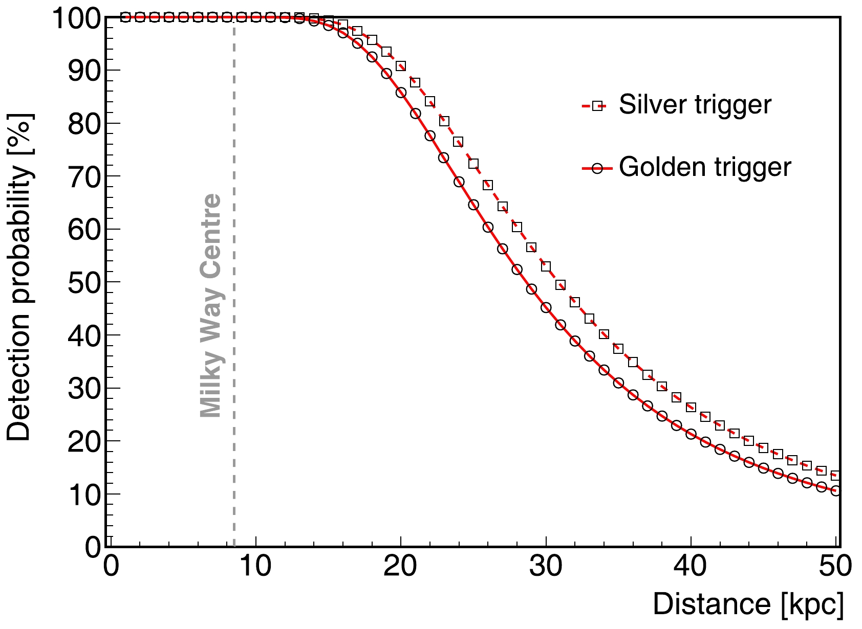
Figure 6. (color online) Detection probability of the SN explosion as a function of distance from the SN to Earth. The Garching model is used with
$ M_{p}=27\; M_{\odot} $ via the LS220 EoS.We predict that 3.4 false alerts would occur in the physical data in the golden trigger mode and one is observed. The p-value for this downward fluctuation is 14.7%. An upper limit at the 90% confidence level (C.L.) is extracted to be 1.6 using the Feldman-Cousin method [41], which is equivalent to 678.2 per century on the rate of core-collapse supernovae in our galaxy out to 10 kpc.
-
The NR spectra of the CEνNS process from SN neutrinos are investigated in PandaX-4T, leading to the expected number of neutrino events ranging from 6.6 to 13.7 by varying the mass of the progenitor stars and the explosion models at a distance of 10 kpc with a time duration of 10 s in the golden trigger mode. The uncertainties in the parameters of the SN theoretical models will be significantly reduced when future SN explosions are observed by the detectors on Earth. Neutrino detectors can provide an early warning for the multi-messenger astronomy, which can better explain the SN dynamics from different aspects. The algorithm to predict the false alert rate is established and validated using experimental data. It takes several minutes to search for SN bursts for each individual file and a bit longer if candidates falling into two separate files are considered. The detection probability for SN explosions within the Milky Way is given, which suggests that the PandaX-4T detector can monitor SN explosions in the Milky Way. The upper limit of SN bursts at 90% C.L. is determined to be 678.2 per century in our galaxy out to 10 kpc. In the future, the trigger algorithm will be integrated into the online SN monitor system in PandaX-4T, facilitating real-time monitoring of SN bursts in our galaxy.
-
We appreciate the support from the Double First Class Plan of Shanghai Jiao Tong University. We also appreciate the sponsorship from the Chinese Academy of Sciences Center for Excellence in Particle Physics (CCEPP), Hongwen Foundation of Hong Kong, Tencent, New Cornerstone Science Foundation, and Discipline Construction Fund of Shandong University in China. Finally, we thank the CJPL administration and the Yalong River Hydropower Development Company Ltd. for indispensable logistical support and other assistance.
Detecting neutrinos from supernova bursts in PandaX-4T
- Received Date: 2024-03-13
- Available Online: 2024-07-15
Abstract: Neutrinos from core-collapse supernovae are essential for understanding neutrino physics and stellar evolution. Dual-phase xenon dark matter detectors can be used to track explosions of galactic supernovae by detecting neutrinos through coherent elastic neutrino-nucleus scatterings. In this study, a variation of progenitor masses and explosion models are assumed to predict neutrino fluxes and spectra, which result in the number of expected neutrino events ranging from 6.6 to 13.7 at a distance of 10 kpc over a 10-s duration with negligible backgrounds at PandaX-4T. Two specialized triggering alarms for monitoring supernova burst neutrinos are built. The efficiency of detecting supernova explosions at various distances in the Milky Way is estimated. These alarms will be implemented in the real-time supernova monitoring system at PandaX-4T in the near future, which will provide supernova early warnings for the astronomical community.


 Abstract
 HTML
HTML Reference
 Related
 PDF
PDF




 DownLoad: