-
The immortal ΛCDM model is undoubtedly successful in accounting for most current cosmological measurements. However, one parameter has caused considerable trouble for this model. In recent years, the difference in the value of the Hubble constant
$ H_0 $ between the global estimation provided by the standard ΛCDM model and local measurements presents a significant statistical tension. In the latest local measurement reported [1], the SH0ES Team obtained$ H_0 = 73.04 \pm 1.04 $ $ {{\rm{km \;s}}^{-1} {{\rm{Mpc}}}^{-1}} $ at 68% CL with 1.42% uncertainty (hereafter R21) using Cepheids observations. However, the global temperature spectrum of cosmic microwave background (CMB) for$ Planck $ 2018 [2] yields$ H_0 = 67.4 \pm 0.5 \;{{\rm{km \;s}}^{-1} {{\rm{Mpc}}}^{-1}} $ at 68% CL in the flat ΛCDM scenario with six basic parameters. Moreover, these differences have increased gradually, reaching 4.88σ. This problem is commonly called "Hubble tension".Initially, the Hubble constant was estimated from the Hubble law
$ \upsilon = H_0 d $ , a linear relationship between recession velocity of galaxies and its distance from the Earth. We have to admit that the measurement of the Hubble constant is difficult technically. The first estimation of the Hubble constant$ H_0 $ was approximately 500$ {{\rm{km \;s}}^{-1} {{\rm{Mpc}}}^{-1}} $ [3], due to the confusion between two generations of pulsating stars in the calculation of distance standards. In 1921, Leavitt and Pickering [4] found a highly regular period of brightness fluctuation of Cepheid variables. Owing to the period-luminosity relation, Cepheids have been used since then as standard candles. Further improving this method, the SH0ES Team increased the number of geometric calibrations of Cepheids and measured the fluxes of all Cepheids along the distance ladder. Finally, a local measurement was obtained as mentioned earlier. The other independent local measurement was performed by the H0LiCOW team, which focused on the measurement of time delays caused by strong gravitational lensing between multiple images of background quasars and the foreground galaxy. Six of these measurements yielded$ H_0 = 73.3 \pm 1.8\; {{\rm{km \;s}}^{-1} {{\rm{Mpc}}}^{-1}} $ [5]. However, using alternative distance ladders, for example, the local tip of the red giant branch, resulted in$ H_0 = 69.8 \pm 0.6 ({\rm stat}) \pm 1.6 ({\rm sys}) {\rm km \;s^{-1} Mpc^{-1}} $ [6]. Departing from the local measurement at the late universe, the Hubble constant can also be estimated by early universe observations. Recent results based on Baryon Acoustic Oscillations (BAO) from eBOSS DR14 and baryon density measurements from Big Bang Nucleosynthesis (BBN) yielded$H_0 = 67.6 \pm 1.1\; {\rm km \;s^{-1} Mpc^{-1}}$ [7], which is in agreement with the Planck2018 result. Similar estimations were obtained in Refs. [8, 9]. Besides Planck2018, other CMB experiments such as ACTPolDR4 and SPT-3G [10, 11]evidence that the Hubble tension has evolved into a contradiction between the early universe and late universe.The Hubble tension has rapidly attracted a lot of attention [12–17]. In Ref. [18], Freedman states that we are at a crossroad in cosmology. The Hubble tension may signal the need for new physics, a deviation from the standard ΛCDM model, or unrecognized uncertainties. Assuming no experimental systematics, the search for new physics may resolve the tension. Ref. [19] reviewed a great deal of models to reconcile the Hubble tension, encompassing early and late dark energy, modified gravity, inflationary models, etc. In addition to the 6 parameters of the standard ΛCDM model, Ref. [20] investigated 10, 11, and 12 parameters that extend the ΛCDM model, including the spectral
$ \alpha_s $ , dark energy equation of state (EoS w), effective number of relativistic particles$ N_{{{\rm{eff}}}} $ , and sum of neutrino masses$ \sum m_{\nu} $ . It was confirmed that dark energy with EoS$ w< -1 $ solves the Hubble tension. This conclusion has also been reported in Ref. [21]. In an early dark energy model, Ref. [22] obtained$ H_0=69.6^{+1.0}_{-1.3} {{\rm{km \;s}}^{-1} {{\rm{Mpc}}}^{-1}} $ using the datasets$ Planck $ 2018+CMB lensing+BAO+Pantheon, which can resolve the Hubble tension within$ 2.3\sigma $ . An analysis based on early dark energy [23] suggests that a field accounting for ~5% of the total energy density around$ z \sim 5000 $ and diluting faster than radiation afterwards can solve the Hubble tension without unfitting other datasets. Regarding the famous CPL dark energy,$ Planck $ 2018 + Pantheon + BAO yielded$ H_0 = 68.31 \pm 0.82\; {{\rm{km \;s}}^{-1} {{\rm{Mpc}}}^{-1}} $ [2], which means a$ 3.2\sigma $ tension with R21. However, phenomenologically emergent dark energy with$w=-1- [1+ \tanh (\log_{10}(1+z))]/ ({3 \ln 10})$ [24, 25] under full Planck2015 CMB analysis yielded$ H_0=72.58^{+0.79}_{-0.80} \;{{\rm{km \;s}}^{-1} {{\rm{Mpc}}}^{-1}} $ [26], which improves the Hubble tension to$ 1\sigma $ . Modified gravity with exponential form$f({\cal{T}}) = -{\cal{T}} {\rm e}^{\beta({\cal{T}}_0/{\cal{T}})}$ also yields$H_0 = 71.49 \pm 0.47 \; {{\rm{km \;s}}^{-1} {{\rm{Mpc}}}^{-1}}$ under$ Planck $ 2018 + CMB lensing + BAO. Interestingly, interacting dynamical dark energy can further reduce the Hubble tension [27, 28]. These results can also be found in holographic dark energy cosmology [29].In the present study, we tested the Hubble tension through some late dark energy phenomenological models. To further analyze whether the Hubble tension can be alleviated by late dark energy parameterization, we built several ersatz forms including fractional, logarithmic, exponential, and inverse exponential forms. We also investigated the extent to which the Hubble tension is influenced by the types of dark energy. We also constructed several non-parameterized exponential dark energy EoS with
$ w> -1 $ and$ w< -1 $ .This paper is organized as follows. In Section II, we introduce the corresponding dark energy models and observational datasets used in our study. In Section III, we present the reconstruction results and corresponding analysis. Finally, in Section IV, discussion are drawn and conclusions are presented.
-
For a spatially flat FRW Universe, we consider the cosmic components with radiation, matter, and dark energy expressed as
$ H^2(z) = H_0^2 \left[ \Omega_{r} (1+z)^4 + \Omega_{m}(1+z)^3 + \Omega_{\rm DE} (z) \right] , $

(1) where the dark energy density parameter is
$ \Omega_{\rm DE}(z) = (1 - \Omega_{r} - \Omega_{m}) \exp \left[3 \int_0^{z} \frac{1+w(z)}{1+z} {\rm d}z \right]. $

(2) Here,
$ \Omega_{m} $ is the matter density parameter at the present epoch,$ \Omega_{r} $ is the radiation density parameter at the present epoch, and$ w(z) $ is the equation of state of dark energy. To establish a fair test, these parameterizations contain fractional, logarithmic exponential, and inverse exponential forms. The four models are double-free parameter models. Moreover, the EoS is valid across$ w = -1 $ . The equation of state w for dark energy is respectively expressed as follows:$ \begin{aligned}[b] {{\rm{Model}}}\;1 : w \;\;=\;\;& w_0 + w_a \frac{z}{(1+z)^2}, \\ {{\rm{Model}}}\;2 : w \;\;=\;\;& w_0 + w_a \frac{\ln (1+z)}{1+z}, \\ {{\rm{Model}}}\;3 : w \;\;=\;\;& w_0 + w_a \frac{1}{1+z} [e - {\rm e}^{\frac{1}{1+z}}], \\ {{\rm{Model}}}\;4 : w \;\;=\;\;& w_0 + w_a \left[\frac{1}{e} - \frac{1}{1+z} \frac{1}{{\rm e}^{\frac{1}{1+z}}}\right] . \end{aligned} $

(3) For the second objective previously mentioned, we built several nonparametric dark energy models defined to fulfill
$ w > -1 $ or$ w < -1 $ within the proper redshift interval. In other words, Models 5 to 10 defined in Eq. (4) are quintessence-like and phantom-like dark energy models. Moreover, they were constructed step by step to test how much the Hubble tension is influenced by the types of dark energy. The constructions resulted in the following expressions:$ \begin{aligned}[b] {{\rm{Model}}}\;5 : w \;\;=\;\;& -1 + \frac{a}{{\rm e}^a}, \\ {{\rm{Model}}}\;6 : w \;\;=\;\;& -1 - \frac{a}{{\rm e}^a}, \\ {{\rm{Model}}}\;7 : w \;\;=\;\;& -1 + \frac{0.5 a}{{\rm e}^a}, \\ {{\rm{Model}}}\;8 : w \;\;=\;\;& -1 - \frac{0.5 a}{{\rm e}^a}, \\ {{\rm{Model}}}\;9 : w \;\;=\;\;& -1 + \frac{0.2 a}{{\rm e}^a}, \\ {{\rm{Model}}}\;10 : w \;\;=\;\;& -1 - \frac{0.2 a}{{\rm e}^a} . \end{aligned} $

(4) In Section III, we test whether the parameterization can be popularized to
$w = -1 + \dfrac{n a}{{\rm e}^a}$ . That is, we aim to determine the influence of the parameter n on the dark energy. We must clarify that these models are different from those of the popular CPL parameterization. For the latter, EoS is assumed to be$ w(a) = w_0 + w_a (1-a) $ , with a constant change rate${\rm d}w/{\rm d}a = -w_a$ . In contrast, the proposed models exhibit a more complex change rate, which makes these constructions more realistic. For the sake of clarity, their change rate$w' = {\rm d}w/{\rm d}a $ is expressed as follows:$ \begin{aligned}[b] {{\rm{Model}}}\;1 : w' \;\;=\;\;& w_a (1 - 2a), \\ {{\rm{Model}}}\;2 : w' \;\;=\;\;& - w_a [\ln(a) + 1], \\ {{\rm{Model}}}\;3 : w' \;\;=\;\;& w_a (e - {\rm e}^a - a {\rm e}^a ), \\ {{\rm{Model}}}\;4 : w' \;\;=\;\;& w_a \left(\frac{a}{{\rm e}^a} - \frac{1}{{\rm e}^a} \right), \\ {{\rm{Model}}}\;5 : w' \;\;=\;\;& (1-a) {\rm e}^{-a}, \\ {{\rm{Model}}}\;6 : w' \;\;=\;\;& -(1-a) {\rm e}^{-a}, \\ {{\rm{Model}}}\;7 : w' \;\;=\;\;& 0.5 (1-a) {\rm e}^{-a}, \\ {{\rm{Model}}}\;8 : w' \;\;=\;\;& -0.5 (1-a) {\rm e}^{-a}, \\ {{\rm{Model}}}\;9 : w' \;\;=\;\;& 0.2 (1-a) {\rm e}^{-a}, \\ {{\rm{Model}}}\;10 : w' \;\;=\;\;& -0.2 (1-a) {\rm e}^{-a} . \end{aligned} $

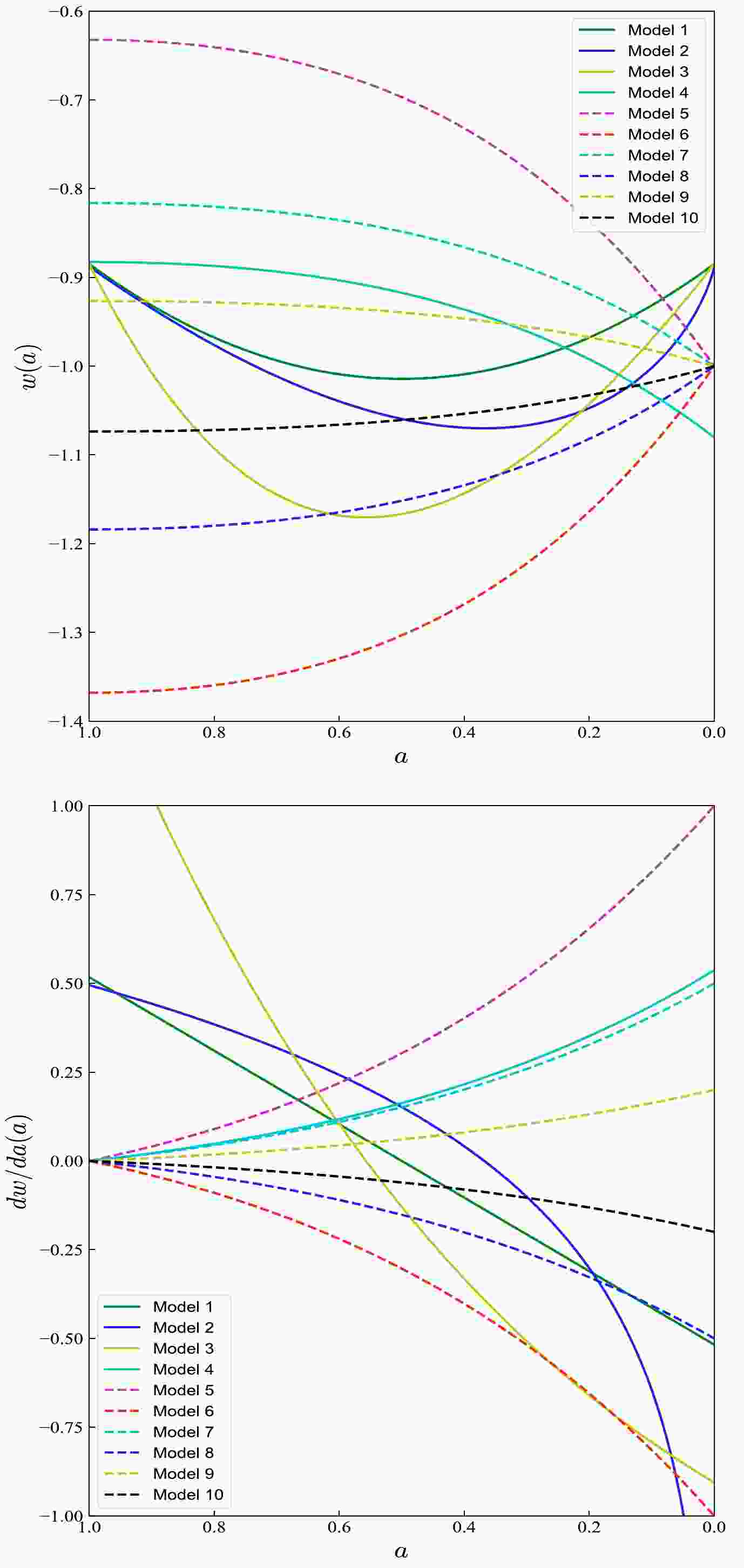
(5) Note that our parameterizations describe the dynamic evolution of dark energy. As shown in Fig. 3, they exhibit significant evolutionary properties. In Section III, we further discuss these aspects.
We used the following observational datasets:
● PR4: The CMB has been one of the most powerful approaches to study the cosmology and physics of the early universe. We used the latest Planck DR4 likelihoods, released in 2020 and named as NPIPE pipeline by the Planck intermediate results LVII [30] (hereafter PR4). PR4 has been utilized in the modified gravity and CMB lensing analysis [31–33]. The PR4 release includes the high-
$ \ell $ Plik TT likelihood spanning over the multipole range$ 30 \leq \ell \leq 2508 $ , as well as TE and EE measurements within the multipole range$ 30 \leq \ell \leq 1996 $ . The multi-frequency multi-component likelihood function for the template fitting can be expressed as$ -2\ln {\cal{L}} \left(\hat{C}|C(\theta) \right) = \left[ \hat{C} - C(\theta) \right]^T \Sigma^{-1} \left[ \hat{C} - C(\theta) \right] , $

(6) where
$ \hat{C} $ is the vector with observed power spectrum,$ C(\theta) $ represents the predicted spectra for the cosmological parameter set θ, and Σ is the covariance matrix computed for a fiducial realization.● Pantheon+: Pantheon+, an update of the Pantheon catalog [34], is the latest sample of SNe Ia. It consists of 1701 SNe Ia light curves observed from 1550 distinct SNe with redshift range of
$ 0.001 < z < 2.26 $ [35]. The Pantheon+ compilation is characterized by significant enhancements, not only because of its expanding sample size, particularly for SNe at redshifts below 0.01, but also in terms of systematic uncertainties. For the Pantheon+ sample, the corresponding optimization function can be expressed as$ -2\ln {\cal{L}} = \Delta \mu \, \mathrm{C^{-1}_{stat+sys}} \, \Delta \mu^T , $

(7) where
$ \Delta \mu = \left[\mu_{{{\rm{obs}}}}(z_i) - \mu_{{{\rm{th}}}}(\theta, z_i) \right] $ is the difference between the observational distance modulus$ \mu_{{{\rm{obs}}}} $ and theoretical distance modulus$ \mu_{{{\rm{th}}}} $ at each redshift$ z_i $ , and$ \mathrm{C_{stat+sys}} $ represents the covariance matrix of the Pantheon+ dataset, including both systematic and statistical uncertainties. The theoretical distance modulus$ \mu_{{{\rm{th}}}} (\theta, z_i) $ is expressed as$ \mu_{{{\rm{th}}}} (\theta, z_i) = 5\log_{10} \frac{d_L (\theta, z_i)}{{{\rm{Mpc}}}} + 25 $

(8) with luminosity distance
$d_L = (1+z) \int^{z}_0 \dfrac{{\rm d}z'}{H(z')}$ .● BAO: Following Ref. [2], we used the Baryon Acoustic Oscillation compilation, which consists of data from the 6dFGS [36], SDSS MGS [37], and BOSS DR12 [38] surveys, summarized in Table IV of Ref. [39]. For the BAO dataset, the corresponding likelihood can be expressed as
$ \begin{aligned}[b] -2\ln {\cal{L}} \;\;=\;\; \sum_{ij} {\bf{d}}_i C^{-1}_{ij} {\bf{d}}^{T}_j +\;\; \left[\frac{r_{{{\rm{drag}}}}/D_V(0.106) - 0.336}{0.015} \right]^2 \end{aligned} $

$ \begin{aligned}[b] +\;\; \left[\frac{r_{{{\rm{drag}}}}/D_V(0.15) - 4.46}{0.17} \right]^2 , \end{aligned} $

(9) where the vector
$ {\bf{d}} $ is a combination expressed as follows:$ \begin{aligned}[b] {\boldsymbol{d}} \equiv & \left( r_{d, {{\rm{fid}}}}\frac{D_M(z_1)}{r_{{\rm{drag}}}}, H(z_1)\frac{r_{{\rm{drag}}}}{r_{d, {{\rm{fid}}}}}, r_{d, {{\rm{fid}}}}\frac{D_M(z_2)}{r_{{\rm{drag}}}}, \right. \\ & \left. H(z_2)\frac{r_{{\rm{drag}}}}{r_{d, {{\rm{fid}}}}}, r_{d, {{\rm{fid}}}}\frac{D_M(z_3)}{r_{{\rm{drag}}}}, H(z_3)\frac{r_{{\rm{drag}}}}{r_{d, {{\rm{fid}}}}} \right). \end{aligned} $

(10) Here,
$r_{{\rm{drag}}} = \displaystyle\int_{z_{{\rm{drag}}}}^\infty \dfrac{{\rm d}z}{\sqrt{3(1+R)}H(z)}$ is the comoving sound horizon and$ D_V(z) \equiv \left[D_M^2(z)\dfrac{z}{H(z)}\right]^{1/3} $ is the spherically averaged BAO distance, with$D_M = \displaystyle\int_{0}^{z} \dfrac{c {\rm d} z'}{H(z')}$ .In the proposed cosmological models, the parameter spaces are defined by the baryon energy density
$ \Omega_b h^2 $ , cold dark matter energy density$ \Omega_c h^2 $ , ratio between the sound horizon and angular diameter distance at decoupling$ 100\theta_{{{\rm{MC}}}} $ , reionization optical depth τ, spectral index$ n_s $ , amplitude of the scalar primordial power spectrum$ A_s $ , and two dark energy parameters, namely$ w_0 $ and$ w_a $ , assumed in our EoS parameterization.We obtained cosmological parameter constraints using the Einstein-Boltzmann code
${\mathrm{CLASS}}$ [40] interfaced with the${\mathrm{Montepython-v3}}$ Monte Carlo sampler [41, 42], which is a publicly available package based on the Markov chain Monte Carlo Chain. The analysis of the MCMC chains to compute the posterior constraints was performed with the Python package GetDist [43] and Gelman-Rubin criterion$ R-1<0.01 $ . -
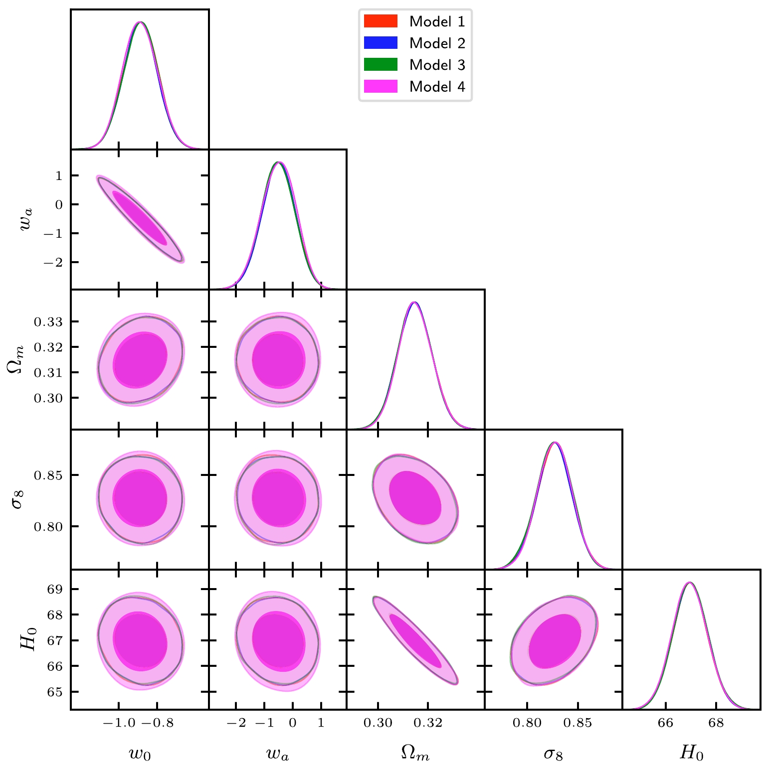
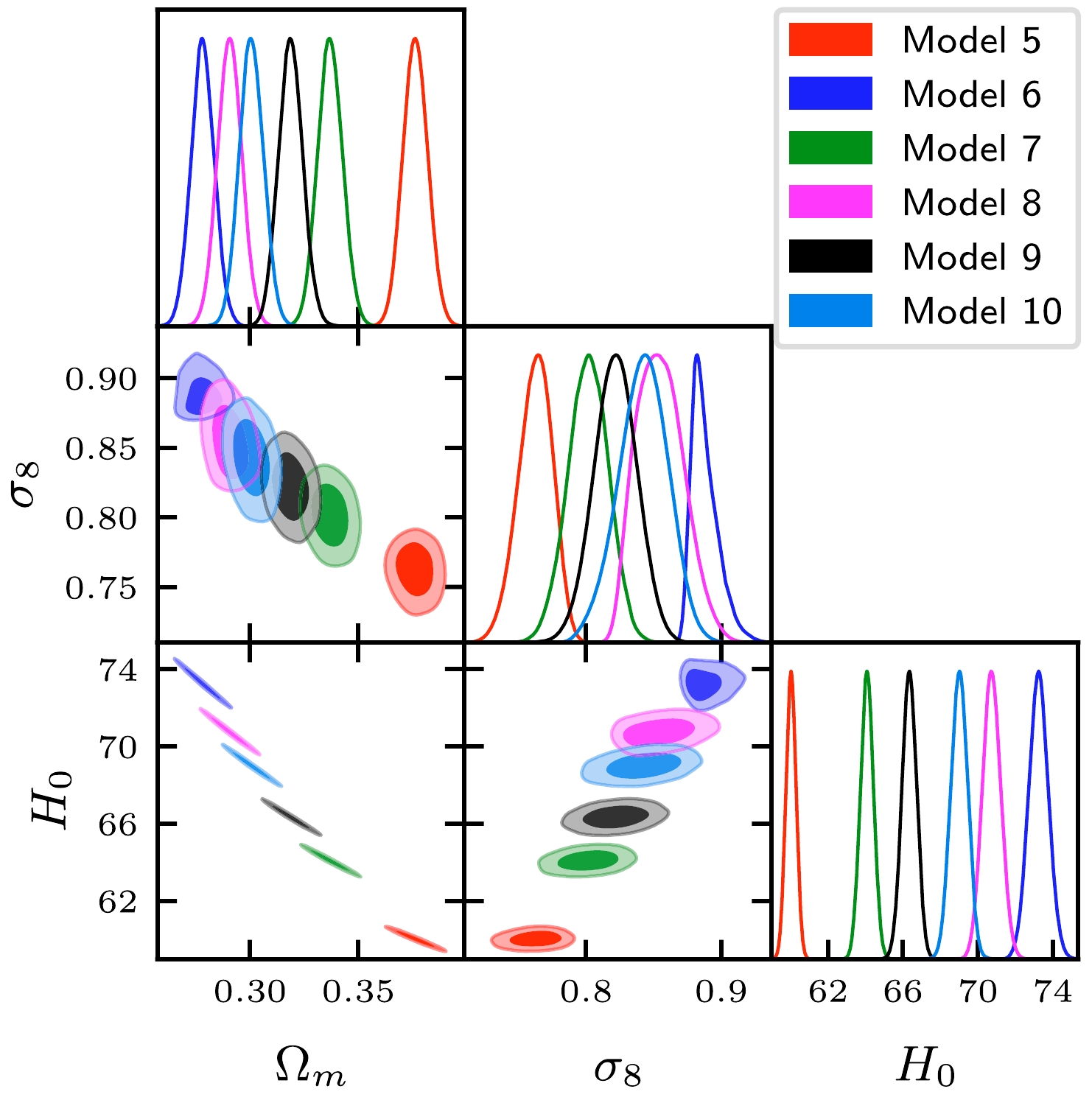
We next present the corresponding results in Table 1, Table 2 and contour constraints in Figs. 1−2.
Parameters Model 1 Model 2 Model 3 Model 4 $ 100\Omega_b h^2 $ 

$ 2.23071\pm0.01461 $ 

$ 2.23083\pm0.01479 $ 

$ 2.23035\pm0.01514 $ 

$ 2.2303410\pm0.01499 $ 

$ \Omega_c h^2 $ 

$ 0.11821\pm0.00120 $ 

$ 0.11818\pm0.00120 $ 

$ 0.11824\pm0.00123 $ 

$ 0.11822\pm0.00120 $ 

$ 100\theta_{s} $ 

$ 1.04185\pm0.00024 $ 

$ 1.04186\pm0.00023 $ 

$ 1.04184\pm0.00023 $ 

$ 1.04185\pm0.00023 $ 

$ \ln (10^{10} A_s) $ 

$ 3.11756\pm0.04536 $ 

$ 3.11789\pm0.04471 $ 

$ 3.11532\pm0.04624 $ 

$ 3.11664\pm0.04599 $ 

$ n_s $ 

$ 0.96843\pm0.00468 $ 

$ 0.96846\pm0.00453 $ 

$ 0.96824\pm0.00462 $ 

$ 0.96840\pm0.00471 $ 

τ $ 0.09452\pm0.02338 $ 

$ 0.09470\pm0.02310 $ 

$ 0.09344\pm0.02382 $ 

$ 0.09411\pm0.02368 $ 

$ w_0 $ 

$ -0.88491\pm0.08990 $ 

$ -0.88781\pm0.08874 $ 

$ -0.88464\pm0.09045 $ 

$ -0.88251\pm0.09019 $ 

$ w_a $ 

$ -0.51737\pm0.59760 $ 

$ -0.49518\pm0.58214 $ 

$ -0.52728\pm0.60155 $ 

$ -0.53692\pm0.59910 $ 

$ \Omega_{m} $ 

$ 0.31482\pm0.00685 $ 

$ 0.31480\pm0.00685 $ 

$ 0.31464\pm0.00689 $ 

$ 0.31467\pm0.00673 $ 

$ \sigma_8 $ 

$ 0.82696\pm0.01732 $ 

$ 0.82677\pm0.01701 $ 

$ 0.82648\pm0.01755 $ 

$ 0.82685\pm0.01731 $ 

$ H_0 $ 

$ 66.97320\pm0.69100 $ 

$ 66.96889\pm0.68951 $ 

$ 66.99802\pm0.69565 $ 

$ 66.98967\pm0.68221 $ 

$ - \ln {\cal{L}}_{{{\rm{max}}}} $ 

6326.20 6326.58 6326.66 6326.37 ΔAIC 0.80 1.56 1.72 1.14 tension 4.8588σ 4.8654σ 4.8289σ 4.8644σ Table 1. Constraints of cosmological parameters at 68% C.L. for different models using all the observational datasets. The parameter
$H_0$ is measured in units of km s−1Mpc−1.Parameters Model 5 Model 6 Model 7 Model 8 Model 9 Model 10 ΛCDM $ 100\Omega_b h^2 $ 

$ 2.27909\pm0.01384 $ 

$ 2.16075\pm0.01200 $ 

$ 2.25536\pm0.01376 $ 

$ 2.19204\pm0.01310 $ 

$ 2.23877\pm0.01352 $ 

$ 2.21253\pm0.00013 $ 

$ 2.22643\pm0.01341 $ 

$ \Omega_c h^2 $ 

$ 0.11211\pm0.00098 $ 

$ 0.12691\pm0.00083 $ 

$ 0.11512\pm0.00094 $ 

$ 0.12282\pm0.00089 $ 

$ 0.11720\pm0.00093 $ 

$ 0.12036\pm0.00092 $ 

$ 0.11874\pm0.00093 $ 

$ 100\theta_{s} $ 

$ 1.04235\pm0.00023 $ 

$ 1.04123\pm0.00023 $ 

$ 1.04209\pm0.00023 $ 

$ 1.04152\pm0.00023 $ 

$ 1.04193\pm0.00023 $ 

$ 1.04169\pm0.00023 $ 

$ 1.04182\pm0.00023 $ 

$ \ln (10^{10} A_s) $ 

$ 3.24692\pm0.03537 $ 

$ 2.98024\pm0.02200 $ 

$ 3.18203\pm0.03916 $ 

$ 3.02208\pm0.04090 $ 

$ 3.13935\pm0.04077 $ 

$ 3.07215\pm0.04429 $ 

$ 3.10599\pm0.04229 $ 

$ n_s $ 

$ 0.98687\pm0.00418 $ 

$ 0.94636\pm0.00366 $ 

$ 0.97751\pm0.00407 $ 

$ 0.95577\pm0.00400 $ 

$ 0.97130\pm0.00405 $ 

$ 0.96243\pm0.00401 $ 

$ 0.96691\pm0.00405 $ 

τ $ 0.16625\pm0.01821 $ 

$ 0.01693\pm0.01072 $ 

$ 0.13030\pm0.02012 $ 

$ 0.04191\pm0.02064 $ 

$ 0.10655\pm0.02074 $ 

$ 0.06960\pm0.02251 $ 

$ 0.08816\pm0.02154 $ 

$ w_0 $ 

−0.63212 −1.36787 −0.81606 −1.18393 −0.92642 −1.07357 −1 $ w_a $ 

– – – – – – – $ \Omega_{m} $ 

$ 0.37627\pm0.00578 $ 

$ 0.27806\pm0.00534 $ 

$ 0.33699\pm0.00566 $ 

$ 0.29059\pm0.00558 $ 

$ 0.31874\pm0.00560 $ 

$ 0.30075\pm0.00567 $ 

$ 0.30888\pm0.00565 $ 

$ \sigma_8 $ 

$ 0.76226\pm0.01257 $ 

$ 0.88780\pm0.01000 $ 

$ 0.80143\pm0.01486 $ 

$ 0.85460\pm0.01726 $ 

$ 0.82170\pm0.01607 $ 

$ 0.84210\pm0.01812 $ 

$ 0.83244\pm0.01695 $ 

$ H_0 $ 

$ 60.02244\pm0.27084 $ 

$ 73.25048\pm0.52318 $ 

$ 64.07296\pm0.34584 $ 

$ 70.74186\pm0.48808 $ 

$ 66.33607\pm0.38979 $ 

$ 68.99304\pm0.45334 $ 

$ 67.72512\pm0.42332 $ 

$ - \ln {\cal{L}}_{{{\rm{max}}}} $ 

6395.95 6415.85 6339.03 6355.59 6326.79 6334.47 6327.80 ΔAIC 136.30 176.10 22.46 55.58 2.02 13.34 – tension $ 12.1129\sigma $ 

0.1808σ $ 8.1816\sigma $ 

2.0004σ $ 6.0361\sigma $ 

3.5671σ 4.7334σ Table 2. Constraints of cosmological parameters at 68% C.L. for different models using all the observational datasets. The parameter
$H_0$ is measured in units of km s−1Mpc−1. -
For the fractional-form Model 1, expressed as
$w = w_0 + w_a z/ (1+z)^2$ , the datasets present a moderate baryon energy density parameter$100\Omega_{b}h^2 = 2.23071\pm 0.01461$ , which is consistent with the constraint$\Omega_{b}h^2 = 0.0224 \pm 0.0001$ from Planck2018 in the standard ΛCDM model [2]. For the other basic parameters, i.e.,$ \Omega_{c}h^2 $ ,$ n_s $ , etc., they are also consistent with the Planck2018 results [2]. However, note that the reionization optical depth τ is slightly larger than that of the Planck results. Finally, the derived matter density parameter$ \Omega_m = 0.31482 \pm 0.00685 $ is consistent with the Planck2018 result, i.e.,$\Omega_m = 0.3166 \pm 0.0084$ . The late-time fluctuation amplitude parameter$\sigma_8 = 0.82696 \pm 0.01732$ is slightly larger than the Planck2018 constraint,$ \sigma_8 = 0.8120 \pm 0.0073 $ . The Hubble constant$H_0 = 66.97320 \pm 0.69100 {{\rm{km \;s}}^{-1} {{\rm{Mpc}}}^{-1}}$ is also moderate. Comparing with the R21 results, the Hubble tension can reach a$ 4.8588\sigma $ level. We conclude that the Hubble tension in this model is still significant. Focusing on the dark energy EoS, we found that it is quintom-like dark energy transferring from$ w< -1 $ to$ w> -1 $ , as shown in Fig. 3.For the natural-logarithm-form Model 2, expressed as
$ w = w_0 + w_a \ln (1+z)/(1+z) $ , we found that the corresponding constraints are similar to the former model, as shown in Fig. 1. The fundamental parameters take similar values, except for the dark energy EoS$ w_a $ . The fluctuation amplitude parameter is$ \sigma_8 = 0.82677 \pm 0.01701 $ , which is still slightly larger than the Planck2018 constraint. Correspondingly, the Hubble constant is$H_0 = 66.96889 \pm 0.68951 \;{{\rm{km \;s}}^{-1} {{\rm{Mpc}}}^{-1}}$ . Comparing with R21, there exists a$ 4.8654\sigma $ tension, which is still severe. Therefore, we cannot optimistically conclude that the natural-logarithm-form model can relax or solve the Hubble tension.For the exponential-form Models 3 and 4, the constraints are also similar to those of the above models. Moreover, the degeneracies between parameters are also consistent with the above models, as shown in Fig. 1. Finally, we found that the Hubble constant tension in these models is still significant, exceeding
$ 4.8\sigma $ .According to the upper panel of Fig. 3, observational datasets in these four parameterizations all present a dark energy transferring from
$ w<-1 $ to$ w>-1 $ . Moreover, their current values are consistent, all pointing towards$ w_0 \simeq -0.9 $ . Concerning the change rate of EoS, given by${\rm d}w/ {\rm d}a$ , we found that Models 1−3 exhibit an increasing derivative. By contrast, the derivative of Model 4 decreases, as shown in the lower panel of Fig. 3. In short, regardless of whether the derivative is greater than zero or changes from${\rm d}w/ {\rm d}a < 0$ to$ {\rm d}w/{\rm d}a >0 $ , the Hubble problem cannot be reconciled.Model 5 is a quintessence-like dark energy model. Its EoS satisfies
$ w > -1 $ . Fig. 2 shows the corresponding contour constraint. Regarding the basic cosmological parameters, it yields slightly larger estimations than the standard ΛCDM model, in particular for the reionization optical depth τ. As a result, we have a higher matter density parameter$ \Omega_m $ and a lower fluctuation amplitude parameter$ \sigma_8 $ . Finally, it yields a smaller estimation of the Hubble constant:$ H_0 = 60.02244 \pm 0.27084 \; {{\rm{km \;s}}^{-1} {{\rm{Mpc}}}^{-1}} $ . The Hubble tension is$ 12.1129\sigma $ , which is the greatest among all the considered dark energy models. Fig. 3 shows that the EoS is also the largest. The current value has reached$ w_0 = -0.63212 $ . That is to say, the larger EoS$ w(a) $ , the more unfavorable it becomes for the Hubble tension.Model 6 is a phantom-like dark energy model. It exhibits evident differences regarding the six basic parameters, especially for the reionization optical depth τ. Concerning the baryon matter, this model yields a lower energy density
$ 100\Omega_b h^2 = 2.16075 \pm 0.01200 $ than the constraint$ \Omega_b h^2 = 0.02236 \pm 0.00015 $ from the standard ΛCDM model [2]. In contrast, the cold dark matter energy density$ \Omega_c h^2 = 0.12691\pm 0.00083 $ is larger. As a result, it favors a smaller matter density parameter$\Omega_m = 0.27806 ±\pm 0.00534$ and a much larger fluctuation amplitude parameter$ \sigma_8 $ . Finally, we obtained an estimation of$ H_0 = 73.25048 \pm 0.52318\; {{\rm{km \;s}}^{-1} {{\rm{Mpc}}}^{-1}} $ . The Hubble tension is reduced to$ 0.1808\sigma $ . This result is encouraging. The current EoS is approximately equal to$ w_0 = -1.36 $ , which is much smaller than the value from other models, as shown in Fig. 3. Its change rate${\rm d}w/ {\rm d}a < 0$ is also the smallest. This result may depart too much from what was expected. Nevertheless, this erratic behavior was also obtained in Ref. [44] when studying a one-parameter dynamical dark energy model. All in all, we consider that the late dark energy influences the estimation of the reionization and Hubble constant.Models 7 to 10 are quintessence-like dark energy models that exhibit a larger baryon matter energy density
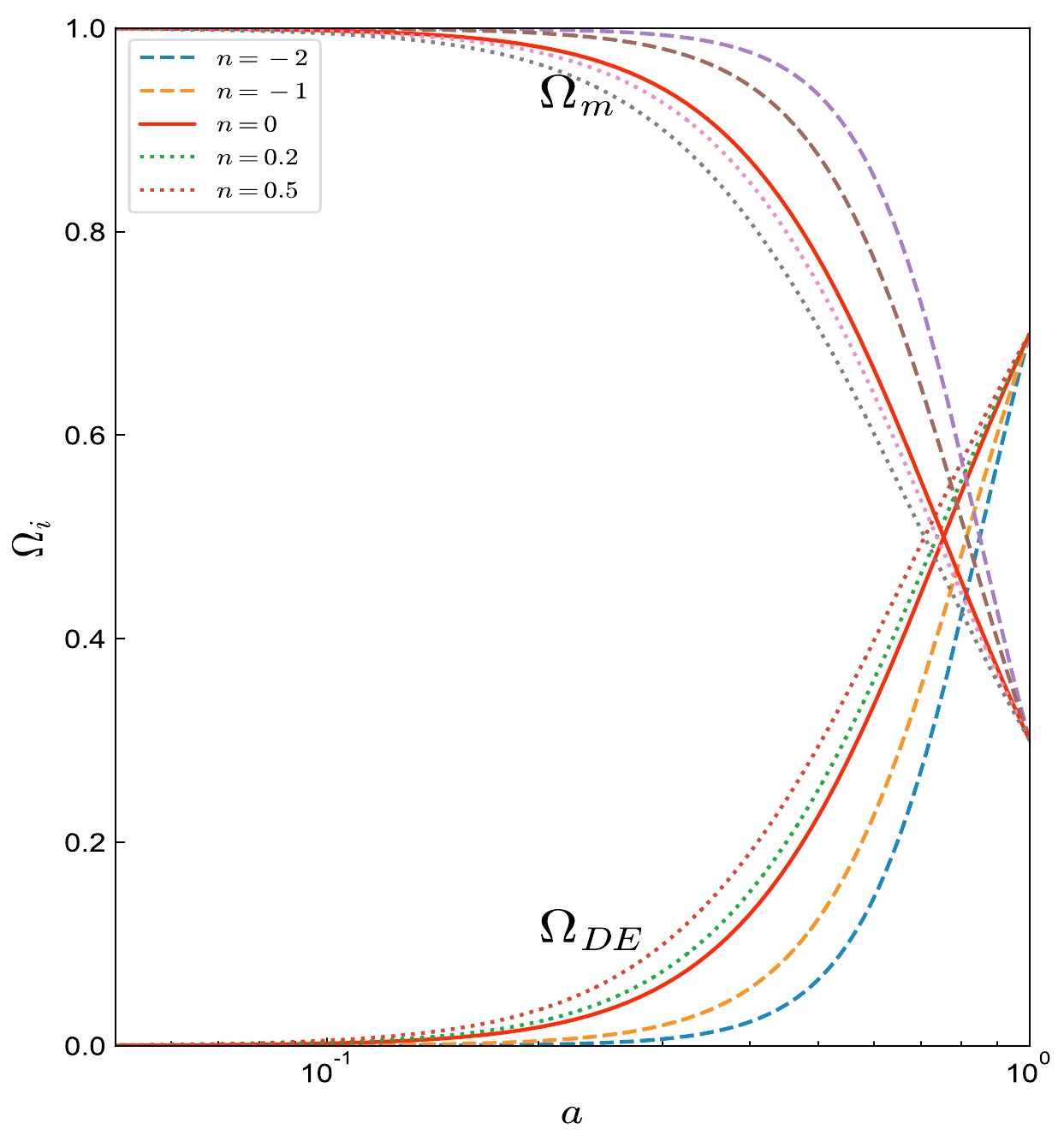
$ 100\Omega_b h^2 $ and$ \Omega_m $ than the phantom-like model. Regarding the Hubble constant, the values from the former models are clearly lower than the values from the latter models. Although phantom-like models seem superior to quintessence-like dark energy models, the Hubble tension of Model 10 approximately reaches$ 3.56\sigma $ . At this point, a question arises. Could we change the value of EoS to be$w = -1 + \dfrac{n a}{{\rm e}^a}$ to reduce the Hubble problem? By comparison, we found that the faster n decreases, the smaller the derivative${\rm d}w/ {\rm d}a$ , and the more relaxed the Hubble problem becomes. We used Eq. (2) to test the influence of the parameter n on the dark energy. Fig. 4 shows that as the parameter n decreases, the dark energy density parameter$ \Omega_{DE} $ decreases and the matter density increases. This affects our estimation about when the dark energy will dominate. -
In Fig. 3, we plot the EoS for different dark energy models to make a comparison. We found that the observational data favor a transformation from
$ w < -1 $ to$ w > -1 $ for the four parameterized dark energy models rather than a transformation from$ w > -1 $ to$ w < -1 $ . Unfortunately, they cannot reconcile the Hubble tension effectively. We also confirmed that Models 5 to 10 have a completely different EoS from the parameterized dark energy Models 1−4. Which model favors the data the most? A model comparison is required.To analyze the Hubble tension, Fig. 5 shows the CMB temperature power spectrum
$ D^{TT}_{\ell} = \ell (\ell +1) C^{TT}_{\ell}/2\pi $ and Fig. 6 depicts the matter power spectrum$ P(k) $ for different dark energy models using the mean values in Tables 1 and 2. We compared the fractional change in CMB temperature power spectrum$\Delta D^{TT}_{\ell}/ D^{TT}_{\Lambda\rm CDM}$ and in matter power spectrum$\Delta P/P_{\Lambda\rm CDM}$ with respect to the ΛCDM model. The corresponding power spectra were computed numerically using${\mathrm{CLASS}}$ [40]. The dots with error bars are observational data with their corresponding uncertainties from Planck2018 [2]. The power spectrum$ C^{TT}_{\ell} $ in different models is consistent with the observational data and exhibits a similar behavior, except for the low multipole$ \ell < 10^1 $ , shown in the upper panel. Note that the heights of the first acoustic peak in the CMB TT spectrum are similar. The spectra for different models have significant differences. As shown in the lower panel of Fig. 5, the ratio indicates that Models 1−4 present a smaller power spectrum than the ΛCDM model. In contrast, Models 5−10 present evident differences in the spectrum. In particular, for Models 5 and 6, the ratio can reach 10%. We conclude that the largest contributions of degeneracies between dark energy models and the ΛCDM model come from the low-multipole$ \ell $ . This phenomenon is also expected in Refs. [2, 45]. Finally, we found that Models 5 and 6 produce a major deviation from the standard ΛCDM model. Concerning the matter power spectrum$ P(k) $ shown in Fig. 6, we found that Models 5 and 6 have the largest deviation from the standard ΛCDM model. This phenomenon is consistent with the CMB temperature power spectrum shown in Fig. 5. Model 2 exhibits the smallest deviation from the standard ΛCDM model. Additionally, note that the differences are mainly reflected in the small k range.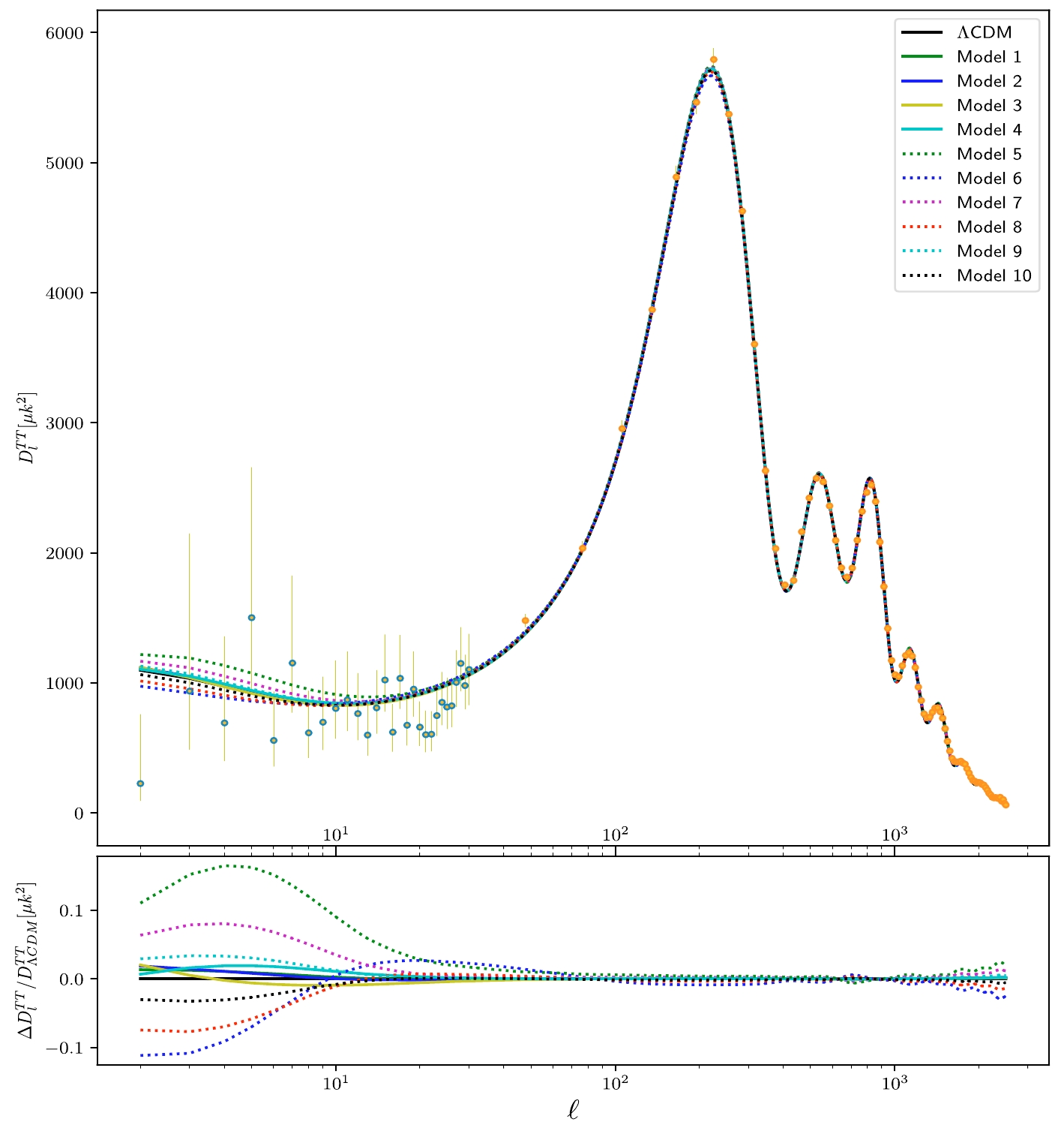
Figure 5. (color online) CMB temperature power spectrum
$ D^{TT}_{\ell} = \ell (\ell +1) C^{TT}_{\ell}/2\pi $ and its fractional change in the temperature spectrum compared with the ΛCDM model for different dark energy models. The dots with error bars are observational data with their corresponding uncertainties from Planck2018 [2].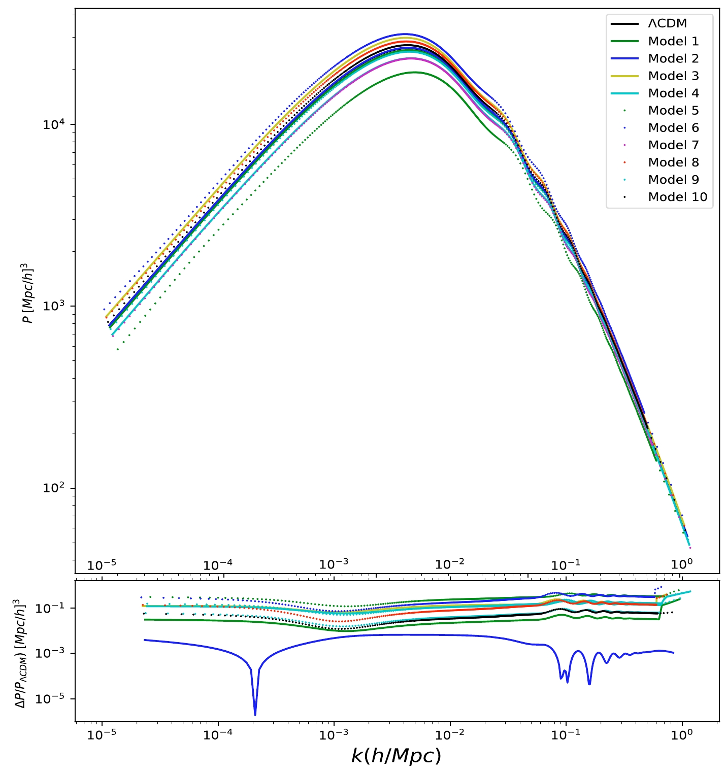
Figure 6. (color online) Matter power spectra
$ P(k) $ and its fractional change in the temperature spectrum compared with the ΛCDM model for different dark energy models.Although the Hubble tension has been relaxed, which model is more supported by the datasets? We performed an Akaike information criterion (AIC) analysis [46]. The AIC is defined as
$ {\rm{AIC}} = -2 \ln {\cal{L}}_{{{\rm{max}}}} + 2\kappa , $

(11) where
$ {\cal{L}}_{{{\rm{max}}}} $ is the maximum likelihood and κ denotes the number of parameters of the model. The best model is that which minimizes the AIC. Commonly, it is tested against the standard ΛCDM model. That is, we consider the analysis ΔAIC = AIC$ _{i} $ - AIC$ _0 $ , where the subscript i denotes the i$ th $ model, and$ 0 $ stands for the ΛCDM model. Therefore, we have a relativistic criterion:$ \Delta {\rm{AIC}} = -2 (\ln {\cal{L}}_{{{\rm{max}}}} - \ln {\cal{L}}_{\Lambda {{\rm{CDM}}}}) + 2(\kappa - \kappa_{\Lambda {{\rm{CDM}}}}) . $

(12) According to MCMC calculations, we have
$ - \ln {\cal{L}}_{\Lambda {{\rm{CDM}}}} = $ 6327.80 in the standard ΛCDM model. The results for ΔAIC are included in Tables 1 and 2. Note that the values of ΔAIC in the four parameterized dark energy models are similar. Note also that the values of ΔAIC in Models 5 and 6 are the worst, although the Hubble tension in Model 6 is the smallest. We can conclude that the resolution of the Hubble tension comes at the cost of AIC. -
The Hubble tension has become a key problem in cosmology. It implies the possibility of new physics or failure of the immortal ΛCDM model. In this paper, we consider ten dark energy models to test whether the models can reconcile the Hubble tension. These models comprise four parameterized dark energy models and several quintessence-like and phantom-like models.
We found that observational data consistently favor a dark energy model transferring from
$ w< -1 $ to$ w > -1 $ for the four parameterizations. However, they are unable to properly reconcile the Hubble tension. We also investigated several nonparametric dark energy models with$ w> -1 $ and$ w<-1 $ . We found that the phantom-like dark energy with$ w < -1 $ can achieve the greatest reduction in Hubble tension to$ 0.1808\sigma $ . Moreover, we found that the change rate of EoS satisfies${\rm d}w/ {\rm d}a < 0$ in the phantom-like models. The current values of the derivative${\rm d}w/ {\rm d}a$ in these models all tend to zero. We obtained relatively large AIC values, which means that the corresponding model is not the most supported one by the datasets. In other words, the resolution of the Hubble tension comes at the cost of high AIC.To establish a fair test, our study model is sufficient. For dark energy parameterization, we considered multiple forms, such as fractional, logarithmic, exponential, and inverse exponential. We found that the determination is less influenced by the dark energy parameterization. We also tested whether the EoS can be popularized to
$w = -1 + \dfrac{n a}{{\rm e}^a}$ . Fig. 4 shows that the parameter n decreases, the dark energy density parameter$ \Omega_{\rm DE} $ decreases, and the matter density increases. This affects our estimation about when the dark energy will dominate.We also investigated the influence of the Hubble tension on the CMB temperature power spectrum
$ C^{TT}_{\ell} $ and matter power spectra$ P(k) $ . We found that Models 5 and 6 exhibit the largest differences on the power spectrum, as shown in Figs. 5 and 6, compared with that of the standard ΛCDM model. These comparisons are consistent with each other.Another point to be emphasized is that the Hubble tension may be related to the estimation of the reionization optical depth τ. It is well known that larger values imply an earlier onset of reionization while
$ \tau = 0 $ implies no reionization at all1 . The history of the reionization process is important given its relevance on how and when the first stars and galaxies formed.The Hubble tension is no longer a contradiction between CMB and supernovae observation but a tension between early universe and late universe. The relevant reasons for this have always been elusive. Our study provides a pertinent result in this regard: alleviation is at the cost of high AIC. As investigated in Ref. [47], future thousands of fast radio bursts could achieve a 3% precision on the random error of the Hubble constant. Gravitational waves and strong gravitational lensing can play an important role in exploring cosmological tensions [48–51]. Using observations of the tidal effect, the BNS/NSBH dark sirens can constrain
$ H_0 $ to 0.2%/0.3% over a five-year observation period [52]. -
We thank the anonymous referee whose suggestions greatly helped us improve this paper. Ming-Jian Zhang thankS Erik Rosenberg and Thejs Brinckmann for the provision of NPIPE calculations and valuable discussion on the PR4.
Can the late dark energy parameterization reconcile the Hubble tension?
- Received Date: 2024-01-14
- Available Online: 2024-07-15
Abstract: In this study, we constructed ten dark energy models to test whether they can reconcile the Hubble tension and how much it is affected by parameterization. To establish a fair test, the models are diverse, encompassing fractional, logarithmic, exponential, and inverse exponential forms as well as several non-parameterized models. The dataset we used includes the NPIPE pipeline of cosmic microwave background (CMB) power-spectrum data from Planck2020, Pantheon+ samples from Supernovae Type Ia, and baryon acoustic oscillations. The MCMC calculations imply dark energy transferring from


 Abstract
 HTML
HTML Reference
 Related
 PDF
PDF






 DownLoad: