Periapsis shift in spherically symmetric spacetimes and effects of electric interactions

I. INTRODUCTION

• I. INTRODUCTION
• II. PRELIMINARIES AND THE NC APPROXIMATION
• III. PS USING THE PN METHOD
• IV. APPLICATIONS TO CHARGED SPACETIMES
•      A PS in RN spacetime
•      B PS in EMD gravity
•      C PS in charged wormhole spacetime
• V. CONSTRAINT ON CHARGES OF KNOWN SYSTEMS
•      A Constraints on solar and Mercury charges
•      B Constraints on Sgr A$^{*}$ and S2 charges
• VI. CONCLUSIONS AND DISCUSSION
• ACKNOWLEDGMENTS
• APPENDIX A: PS IN OTHER SPHERICAL SPACETIMES
•      1 PS with Einstein–Maxwell-scalar field
•      2 PS in charged Horndeski spacetime
•      3 PS in charged black-bounce RN spacetimes

The periapsis shift (PS) of celestial bodies around a central more massive gravity source is an important experimental and theoretical tool for investigating of gravity and the properties of celestial bodies and their orbits. In addition to the famous example of Einstein's explanation of Mercury's extra PS using General Relativity (GR) [1–3], today, the PSs of different types of objects such as satellites [4–7], planets in the solar system [6, 8], and stars around Sgr A^* [9] can be observed experimentally. The PSs of these objects are related not only to the properties of the test particles (such as their charge, spin, or weak interaction with the environment [8]) but also to those of the central object (charge, spin, oblateness, etc. [8–10]), and the nature of the gravity itself [11]. Moreover, the PS is also dependent on the kinetic parameters of the orbits, such as their effective eccentricity e or semilactus rectum p, or equivalently, the specific energy E and angular momentum L.

Among the intrinsic parameters of the spacetime, the effect of central object mass M on the PS is the most well-studied and the result is the well-known Schwarzschild one [1]. The next frequently considered parameter, whose effect on the PS is also observationally important, is the spin angular momentum of the central object, particularly that of those more compact sources. The effect of the electric charge Q of the source on the PS, which is the first motivation of this paper, is less commonly investigated. This parameter is expected to affect the PS of test particles gravitationally through the gravielectric effect. Previously, this effect was considered to always decrease the deflection angle of test particle trajectories in the weak field limit, regardless of the sign of Q [12, 13]. This implies that a nonzero Q would also decrease the PS of test particles. One of the main objectives of this paper is to show that this is true, at least to the leading order of the post-Newtonian (PN) approximation, for all types of electrically charged spacetimes.

A more interesting case is when the test particle is also charged with q, and consequently, both the gravielec-tric and true electrical effects will affect the PS. Moreover, because the electric interaction strength is much stronger than the gravitational one, the charge effect can still be non-negligible even when both the spacetime and particle charges are small. For the electric effect, the sign of Q is important because its product with q, i.e., sign($qQ$) determines the nature of electric interaction; therefore, Q can potentially increase the PS too. This means that an interplay exists between the attractive gravitational and (potentially repulsive) Coulomb interactions. The effect of these interactions and parameters $(Q,\,q)$ on the PS is unclear, and this forms the second motivation of this paper.

When determining the PS under pure gravity, most previous studies used essentially a type of PN approximation, i.e., they assumed that the trajectory is far from the center $(r\gg M)$ and close to an ellipse [14–23]. However, when the trajectory is close to the center, particularly when the center is a black hole, such as Sgr A^*, high order results that were difficult to obtain using the PN approximation might be required to satisfy the required accuracy. In this paper, we develop a near-circular (NC) approximation for orbits that are not very large.

For the PN method, most previous calculations functioned only in specific spacetimes to the leading or at most next-to-leading order of $M/p$ [20, 24–28]. In this paper, we also systematically develop the PN method in general static and spherically symmetric spacetimes with nonzero charges such that both the gravitational and electric interactions can be addressed simultaneously. Additionally, the PS to very high orders can be obtained and linked directly to the asymptotic expansions of the metric functions of the spacetime.

The remainder of this paper is organized as follows. Sec. II introduces the preliminaries, general form of the spacetime and electric field, definition of the PS, NC approximation method, and corresponding result $\alpha_{{\rm{NC}}}$. Sec. III describes the PN treatment of the PS and the result $\alpha_{{\rm{PN}}}$ to arbitrary order. The equivalence of the two approximations are also presented. In Sec. IV, these two methods are applied to the Reissner-Nordström (RN) spacetime, the Einstein-Maxwell dilaton (EMD) gravity, and charged wormhole spacetimes. The PS in each of them is determined, and the effect of the electric interaction is carefully analyzed. Sec. V discusses the constraining of the charge of the solar-Mercury and Sgr A^*-S2 systems using the data of the PS in each system. Sec. VI concludes the paper with a short discussion. Throughout the work, we use the natural system of units $G=c= 4\pi\epsilon_0=1$.

II. PRELIMINARIES AND THE NC APPROXIMATION

• I. INTRODUCTION
• II. PRELIMINARIES AND THE NC APPROXIMATION
• III. PS USING THE PN METHOD
• IV. APPLICATIONS TO CHARGED SPACETIMES
•      A PS in RN spacetime
•      B PS in EMD gravity
•      C PS in charged wormhole spacetime
• V. CONSTRAINT ON CHARGES OF KNOWN SYSTEMS
•      A Constraints on solar and Mercury charges
•      B Constraints on Sgr A$^{*}$ and S2 charges
• VI. CONCLUSIONS AND DISCUSSION
• ACKNOWLEDGMENTS
• APPENDIX A: PS IN OTHER SPHERICAL SPACETIMES
•      1 PS with Einstein–Maxwell-scalar field
•      2 PS in charged Horndeski spacetime
•      3 PS in charged black-bounce RN spacetimes

We study the motion of a charged test particle in the most general static and spherically symmetric spacetime, whose line element is described by

where $(t,r,\theta,\phi)$ are the coordinates, and the metric functions depend on r only. For the electromagnetic field in this spacetime, we assume that only a pure electric field described by the potential $\left[{\cal{A}}_0\left(r\right),0,0,0\right]$ exists. However, in some spacetime solutions with electric fields, no such potential but the electric field itself $E(r)$ is given. Fortunately, for the two methods presented in this paper, we only require the series expansion of ${\cal{A}}_0(r)$ near the orbit radius; therefore, the electric field $E(r)$ is also sufficient. Owing to the symmetry of the spacetime and field, without losing any generality, we can always investigate the equatorial motion of charged test particles in such spacetimes.

The dynamics of a point particle possessing non-zero mass m and specific charge $\hat{q}\equiv q/m$ can be described by the Lorentz equation [29]:

where $F_{\mu\nu}=\partial_\mu A_\nu-\partial_\nu A_\mu$, and τ is the proper time of the test particle. After integrating Eq. (2) on the equatorial plane $(\theta= {\pi}/{2})$, we obtain three first-order differential equations [13]:

where integration constants $\hat{E}$ and $\hat{L}$ correspond to the energy and angular momentum per unit mass of the particle respectively, and $\dot{{}}$ denotes the derivative with respect to proper time τ.

To analyze the radial motion of the particle in more detail, we first rewrite Eq. (3c) in an alternative form:

The zeros and singularities of $B(r)$ and $C(r)$ generally correspond to event horizons or singularities of the spacetime, and in this paper, we focus on region $B(r)C(r)>0$. Thus, we can consider of the first term on the right-hand side of Eq. (4) as a type of effective potential, against which $\hat{L}^2$ can be compared with

Subsequently, the motion of the particle is only allowed when $V(r)\geq \hat{L}^2$. We assume that this inequality has nonempty interval solution $[r_1,\; r_2]$ where

Clearly, $r_1$ and $r_2$ are the radii of the periapsis and apoapsis. For simplicity, we also assume that this interval contains only one local maximum of $V(r)$ at $r=r_c$. For later usage, we denote value$V(r_c)$ as $\hat{L}_c^2$, i.e.,

The existence of such $r_c$ is always possible as long as $\hat{L}^2$ is sufficiently close to $\hat{L}_c^2$. The physical interpretation of $r_c$ is straightforward: it represents the radius of the circular orbit of the particle with energy $\hat{E}$ and angular momentum $\hat{L}_c$. Note that, except for very simple spacetime and electric potential (e.g., the RN spacetime), solving the algebraic equation (7) to obtain the closed form solution of $r_c$ is often difficult. Therefore, in the following sections where $r_c$ is used, we assume that $r_c$ is already solved, numerically if necessary.

With the above consideration, the PS can be defined as

which, after using Eq. (3), becomes

To reveal the effect of electric interaction on the PS, our task becomes to systematically solve the PS in Eq. (9) using appropriate approximations. We present a perturbative approach based on NC approximation, and then in the next section, a PN method is used.

For the NC approximation, the first step for the computation of the integrals in Eq. (9) is to utilize the deviation of the particle's orbit from a perfect circle as a measure of perturbation for series expansion. This deviation can be quantified by parameter a defined as

When $r_1$ and $r_2$ are close, i.e., the orbit is close to a circle, the above defined a will be a small quantity.

To use a, we extend the method developed in Refs. [10, 13, 30] to the case with electric interaction. We first propose a change of variables in Eq. (9) from r to ξ, which are linked by

where function $P(1/r)$ is defined as

From Eq. (7), we observe that function $P(x)$ exhibits opposite monotonic behavior on the two sides of $x=1/r_c$. This implies that its inverse function has two different branches when $x\geqslant 0$. We use $\omega_+$ and $\omega_-$ to denote the branch of the inverse function of $P(x)$ for $r>r_c$ and $r< r_c$ respectively. In other words, using Eq. (11) we obtain

Substituting this change of variables, the terms in the integral (9) become

and consequently the PS in Eq. (9) can be rewritten as

where factor $y(a,\,\xi)$ of the integrand is

An evident advantage of this change of variables is that it transforms two different integral limits $r_1$ and $r_2$ into the same value a and therefore simplifies the computation.

Because we are focusing on the $a\ll 1$ case, the next step is naturally expanding the function $y(\xi)$ for small ξ. Carrying out this expansion, we can show that it generally assumes the form

Here, $y_n(a)$ can be determined once the metric functions and potential ${\cal{A}}_0$ are known around $r_c$. Substituting this back into Eq. (15), and using the integral formula

the PS is computed as

Because we have assumed that deviation parameter a is small, in principle, we can further expand $y_n(a)$ for small a and reorganize the PS into a true power series:

These coefficients $t_n$ are now independent of a and, similar to $y_n$, can be completely determined when the metric functions and electric potential are fixed. In the following, we show this determination process.

We assume that the metric functions and the electric potential ${\cal{A}}_0$ have the following expansions around $r_c$

The definition of $r_c$ in Eq. (7) immediately implies a constraint between these coefficients:

We will use this relation occasionally to simplify $t_n$ and $T_n$ below. Critical $\hat{L}_c$ in Eq. (20) can also be expressed in terms of these coefficients using again Eq. (7):

Substituting the expansions in Eq. (21) into Eq. (12), taking its inverse function $\omega_\pm$ and then substituting it into (16), expanding for small ξ, and eventually expanding $y_n(a)$ again for small a, we an determine coefficients $t_n$ in Eq. (20). Here, for simplicity, we list only the first two:

where $T_n$ represents the n-th derivative of the potential at $r_c$, i.e., $T_n\equiv V^{(n)}(r_c)/n!$, and the first two of them are

The higher order $t_n\; (n=2,\,3,\cdots)$ and $T_n\; (n=4,\,5,\cdots)$ can also be obtained easily using an algebraic system.

In obtaining the PS in Eq. (20), although we used small a or equivalently small eccentricity e approximation, we need not assume that the orbit size itself is large compared with the characteristic length scale (e.g. mass M) of the spacetime. The latter is the key assumption for the PN method, which can also be used to compute the corresponding PS. In next section, we show how the PN method can be used to consider the electric interaction and to determine the PS when the orbit size is large.

III. PS USING THE PN METHOD

• I. INTRODUCTION
• II. PRELIMINARIES AND THE NC APPROXIMATION
• III. PS USING THE PN METHOD
• IV. APPLICATIONS TO CHARGED SPACETIMES
•      A PS in RN spacetime
•      B PS in EMD gravity
•      C PS in charged wormhole spacetime
• V. CONSTRAINT ON CHARGES OF KNOWN SYSTEMS
•      A Constraints on solar and Mercury charges
•      B Constraints on Sgr A$^{*}$ and S2 charges
• VI. CONCLUSIONS AND DISCUSSION
• ACKNOWLEDGMENTS
• APPENDIX A: PS IN OTHER SPHERICAL SPACETIMES
•      1 PS with Einstein–Maxwell-scalar field
•      2 PS in charged Horndeski spacetime
•      3 PS in charged black-bounce RN spacetimes

Many previous studies computed the PS using the PN method. However, most of them, if not all, focused only on the lowest order(s) result, and some used this method very loosely and the results are large. Moreover, only a few of them used the PN method to solve the gravitational and electric interactions simultaneously. In this section, we systematically develop a PN method that not only yields the PS to a high order of the semilatus rectum p but also considers the electric interaction. Some of the techniques we use here are similar to those in Refs. [10, 15, 31]. In the last section, we further show that the PN method result agrees perfectly with the result obtained using the NC method when the orbit size is large and the eccentricity is small.

For the PN method, we first assume that the orbit can be described by the relation

where function $\psi(\phi)$ describes the deviation of the orbit from ellipse. Note that the periapsis and apoapsis of the orbit correspond to $\psi=0$ and $\psi=\pi$ respectively, and radii of the periapsis $r_1$ and apoapsis $r_2$ satisfy

The radius of the orbit evolves for a full period when ψ changes from 0 to $2\pi$; therefore, the PS using this description becomes

${\rm{d}}\phi/{\rm{d}}\psi$ can be expressed from Eq. (26) as

whence we have defined $u=1/r$. Term ${\rm{d}}u/{\rm{d}}\phi$ in Eq. (29) can be transformed using Eq. (3) to

where we have defined the right-hand side as $F(u)$. Next, we show that $F(u)$ can be expressed as a serial function of ψ, and after substituting it back into (28), the integral over ψ can be performed to determine the PS.

The key to accomplishing this is the PN assumption, i.e., we assume that p is large and therefore u is always a small quantity. This enables us to expand $F(u)$ as a power series of u:

where coefficients $f_n$ can be determined from Eq. (30) using the asymptotic expansion of the metric functions and ${\cal{A}}_0$. Assuming that they are of the form

we can then determine $f_n$ order by order as functions of coefficients $a_n,\; b_n,\; c_n$, and $\mathfrak{q}_n$. Here, we only illustrate the first few of them:

Repetitively substituting Eq. (26) as u, all u instances on the right hand side of Eq. (31) can be completely replaced by variables $p,\, e$, and ψ. After collecting terms proportional to $\cos\psi$ and $\sin^{2n}\psi$, we show that $F(u)$ always assumes the form [10]

where $G_0,\; G_0^\prime,\; G_n$ are linear combinations of $f_n$ with coefficients being power series functions of $\hat{E},\; 1/\hat{L},\; e$, and $1/p$. Their exact forms can be dertemined without difficulty although the algebra is too tedious to show here.

Because at the apoapsis and periapsis, by definition (30) we have $F(u)=0$, using the condition (27), we immediately obtain $F(\psi=0)=F(\psi=\pi)=0$, i.e.,

These two power series conditions effectively establish two relations between the kinetic variables $(\hat{E},\, \hat{L})$ and $(p,\, e)$. These conditions can be solved perturbatively when p is large, enabling us to express $(\hat{E},\, \hat{L})$ in terms of $(p,\, e)$

In the final expression for the PS, these expressions can aid us in eliminating the dependence on unnecessary kinetic variables. Note that other methods can be used to obtain the relation between $(\hat{E},\, \hat{L})$ and $(p,\, e)$. Substituting Eq. (27) into Eq. (6), we obtain

Clearly, this is more concise than Eq. (35), and we can show that it is essentially equivalent to Eq. (35).

Now substituting Eq. (35) into Eq. (34) and further into Eq. (29), we find

where, in the second step, we have substituted the first few $G_n\; (n=1,2,\cdots)$ and performed the large p expansion again. Substituting into Eq. (28) and noting that terms proportional to $\cos(k \psi)\; (k=1,2,\cdots)$ will not survive the integration, the result for the PN PS is simply determined as

However, this result is still not a true series of p because of the dependence of $f_n$ on $(\hat{E},\, \hat{L})$ and equivalently on $(p,\, e)$. Substituting Eq. (36) as $f_n$ in Eqs. (33) and re-expanding for large p, we can obtain a true power series form of p for $\alpha_{{\rm{PN}}}$

with the coefficient for order $p^{-n}$, a polynomial of order $2(n-1)$ of eccentricity e. The first few coefficients for $d_{n,j}$ are

Before we analyze the implication of result (40) in the next section, we compare the two PSs, $\alpha_{{\rm{NC}}}$ in Eq. (20) obtained using NC approximation, and $\alpha_{{\rm{PN}}}$. Clearly, these two PSs are only comparable when the orbit is both large and near-circular.

Under this assumption, we now rewrite the PS $\alpha_{{\rm{NC}}}$ using PN kinetic variables $(p,\, e)$. Hence, we must express $(\hat{E},\; \hat{L},\; r_c,\; a)$ in terms of $(p,\, e)$ and other spacetime parameters. First, note that the first two of them, $(\hat{E},\, \hat{L})$, have already been linked to $(p,\, e)$ using Eq. (36). For $r_c$, although the defining Eq. (7) is not always solvable in closed form, it can always be solved perturbatively for large p. Substituting this into Eqs. (36) and asymptotic (32), the solution to$r_c$ as functions of $(p,\, e)$ can be obtained using the method of undetermined coefficients:

Similarly, by substituting Eqs. (36), (32), and (42) into $\hat{L}_c$ in Eq. (7) and further into Eq. (10), small parameter a can also be expressed using $(p,\, e)$ as

Eqs. (42) and (43) enable us to express all terms that depend on $r_c$ and a explicitly in $\alpha_{{\rm{NC}}}$ in Eq. (20) in terms of the asymptotic expansion coefficients $a_n,\,b_n,\,c_n,\,\mathfrak{q}_n$ and kinetic variables $(p,\,e)$. The expansion coefficients of the metric and electric potential functions around $r_c$, i.e., $a_{cn},\,b_{cn},\,c_{cn},\,h_{cn}$, can also be expressed using $a_n,\,b_n,\,c_n,\,\mathfrak{q}_n$ and variables $(p,\,e)$. Hence, we need only to substitute the asymptotic forms (32) and Eq. (42) into the expansion (21) and then further expand these functions for large p. Although $a_{cn},\,b_{cn},\,c_{cn},\,h_{cn}$ can be solved easily, their expressions are too lengthy to present here. Finally, substituting all these coefficients, as well as Eqs. (42) and (43), into Eq. (20), we can express $\alpha_{{\rm{NC}}}$ as power series of $1/p$. Not surprisingly, we find that the result agrees perfectly with the PN formula (40). This agreement demonstrates the correctness of results from both methods. Moreover, for the coefficient of each fixed order of $p^{-n}$, its dependence on the eccentricity e is automatically in a polynomial form, indicating that if the small a expansion in Eq. (20) is performed to high enough order, the rewritten PN result to low orders will be valid even for large e.

IV. APPLICATIONS TO CHARGED SPACETIMES

• I. INTRODUCTION
• II. PRELIMINARIES AND THE NC APPROXIMATION
• III. PS USING THE PN METHOD
• IV. APPLICATIONS TO CHARGED SPACETIMES
•      A PS in RN spacetime
•      B PS in EMD gravity
•      C PS in charged wormhole spacetime
• V. CONSTRAINT ON CHARGES OF KNOWN SYSTEMS
•      A Constraints on solar and Mercury charges
•      B Constraints on Sgr A$^{*}$ and S2 charges
• VI. CONCLUSIONS AND DISCUSSION
• ACKNOWLEDGMENTS
• APPENDIX A: PS IN OTHER SPHERICAL SPACETIMES
•      1 PS with Einstein–Maxwell-scalar field
•      2 PS in charged Horndeski spacetime
•      3 PS in charged black-bounce RN spacetimes

In this section, we implement the two aforementioned methods to determine PSs within several specific spacetimes and investigate the effect of the electric interaction and other spacetime parameters on these shifts.

A PS in RN spacetime

• I. INTRODUCTION
• II. PRELIMINARIES AND THE NC APPROXIMATION
• III. PS USING THE PN METHOD
• IV. APPLICATIONS TO CHARGED SPACETIMES
•      A PS in RN spacetime
•      B PS in EMD gravity
•      C PS in charged wormhole spacetime
• V. CONSTRAINT ON CHARGES OF KNOWN SYSTEMS
•      A Constraints on solar and Mercury charges
•      B Constraints on Sgr A$^{*}$ and S2 charges
• VI. CONCLUSIONS AND DISCUSSION
• ACKNOWLEDGMENTS
• APPENDIX A: PS IN OTHER SPHERICAL SPACETIMES
•      1 PS with Einstein–Maxwell-scalar field
•      2 PS in charged Horndeski spacetime
•      3 PS in charged black-bounce RN spacetimes

The RN spacetime is the simplest and cleanest for the analysis of the PSs of charged particles. However, as we show next, it still captures the main characteristic of the electric interaction effect on the PS. The line element and electric potential of the RN spacetime are given by

Next, we analyze $\alpha_{{\rm{NC}}}$ in Eq. (20) and $\alpha_{{\rm{PN}}}$ in Eq. (40) in this spacetime. First, substituting Eq. (44) into Eq. (7), we see that $r_c$ for the RN spacetime is determined by a quartic polynomial:

Although its solution can still be expressed in a closed form, it is too lengthy to show here [13]. When $r_c$ is determined, using $\hat{L}_c$ in Eqs. (7) and (10), we immediately determine small parameter a:

Using Eq. (24), coefficients $t_n$ for RN spacetime can be determined without much difficulty. After combining with a, we finally obtain $\alpha_{{\rm{NC}}}$ in RN spacetime:

Higher orders can also be determined but are too lengthy to show here. Using a computer algebraic system, we computed this result to the tenth order of a.

To determine the PN PS in RN spacetime, we need only expand the metric functions and electric potential (44) asymptotically and then substitute the coefficients into Eq. (40). These steps are very simple, and the result to order $p^{-2}$ is

where $\hat{Q}\equiv Q/M$ denotes the charge-to-mass ratio of the central object. As indnicated in the last section, when p is large and e is small, this PS should coincide with the NC result $\alpha_{\rm{RN,NC}}$ in Eq. (47). We have converted all $(\hat{E},\, \hat{L})$ instances in $\alpha_{\rm{RN,NC}}$, including those in $r_c$ and a to $(p,\, e)$, and the result agrees perfectly with (48), which is naturally small e expanded. When truncated to first order and set to neutral test particle, Eq. (48) agrees with results in Refs. [14–17, 19–23]. For nonzero $\hat q$, Eq. (48) to the first order agrees with Eq. (28) of Ref. [24] and Eq. (42) of Ref. [28]. However, the results in Refs. [25, 26] cannot be determined from our work.

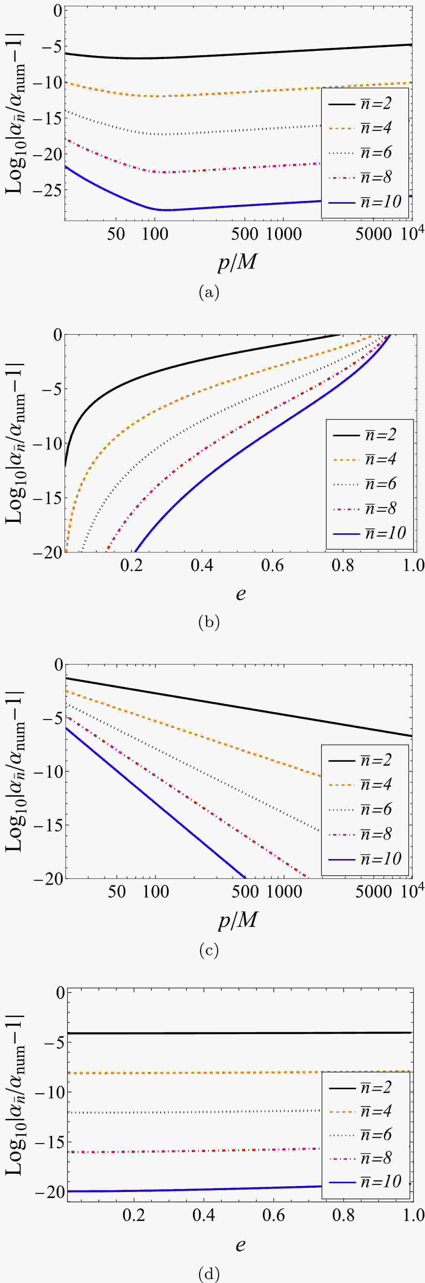
To check the correctness of the PSs in Eqs. (47) and (48), Fig. 1 plots the difference between the series result $\alpha_{\rm{RN,NC}}$ (Fig. 1(a) and 1(b)) and $\alpha_{\rm{RN,PN}}$ (Fig. 1(c) and 1(d)) truncated to order $\bar{n}$ and PS $\alpha_{{\rm{num}}}$ computed using the numerical integration of the definition (8). The latter is performed to very high accuracy and can therefore be considered the true value of the PS. In both plots, we fix $|\hat{Q}\hat{q}|\ll 1$ to ensure that the orbit is a bound one and the PS is well defined. For the NC PS plotted in Fig. 1(a) and 1(b), although $\alpha_{\rm{RN,NC}}$ only explicitly depends on $(\hat{E},\, \hat{L})$, we still convert them to $(p,\, e)$ using Eq. (36) to make a comparison with Fig. 1(c) and 1(d) for PN PS $\alpha_{\rm{RN,PN}}$. Note that in Fig. 1(a) and 1(c), p is varied, whereas in Fig. 1(b) and 1(d), e is changed.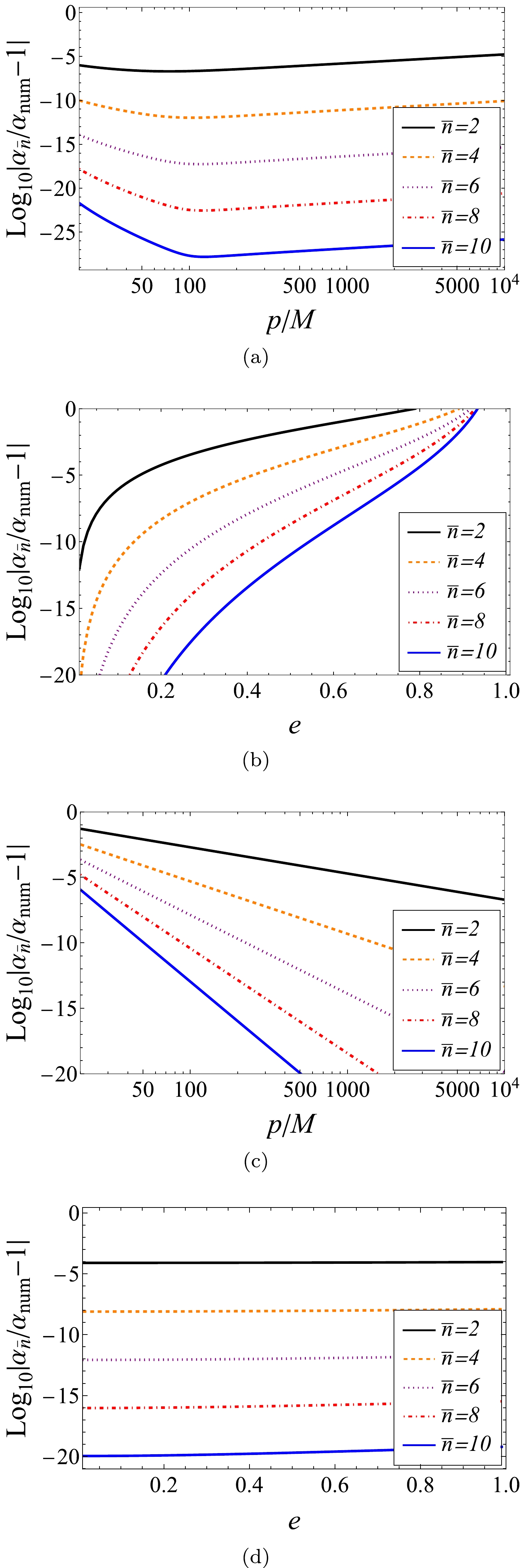

Figure 1

Figure 1.  (color online) Differences between the numerical and analytic results in Eqs. (47) and (48) truncated to order $\bar{n}$, with parameters fixed at $\hat{Q}=1/2,\hat{q}=-1/5,p=500M,e=1/10$, except for the running one.

DownLoad: Full-Size Img PowerPoint

All the plots in Fig. 1 show that as the truncation order increases, both the NC and PN results approach the true value of the PS exponentially. This shows that both methods are effective as the series order increases. Moreover, for $\alpha_{\rm{RN,NC}}$ Fig.1(a) shows that when e is small, the NC approximation almost functions equally well for large p and small p, and Fig. 1(b) shows that this method is very sensitive to e. The smaller the e, i.e, the more circular the orbit is, the more accurate the $\alpha_{\rm{RN,NC}}$. In contrast, we observe that the characteristics of plots Fig.1(c) and 1(d) are the opposite of those of Fig.1(a) and 1(b): the accuracy of $\alpha_{\rm{RN,PN}}$ is not sensitive to e but increases rapidly as p increases. Again, this corresponds with the expectation of a PN approximation of the orbit. The abovementioned characteristics were also observed in Ref. [10], where the effect of the spacetime spin was studied.

Effect of $\hat{q}$ and $\hat{Q}$ on PS

With the correctness of the PS, particularly the PN PS (48), verified, we can now use it to analyze the physics contained in this formula. A few points must be noted. First, this PS depends on parameters $q,\; m,\; Q,\; M$ only through the two charge-to-mass ratios $\hat q$ and $\hat Q$, indicating a certain redundancy in these parameters. Therefore, in the following, when analyzing the effects of these parameters, we need only focus on these two ratios. Second, the charge q appears only in the form of $(qQ)^n$, showing that q influences the PS only through the Coulomb interaction. Q also manifests in terms that are not a product with q; therefore, it can affect the PS through the gravitational channel. Third, because this result is post-Newtonian, it is more accurate in the asymptotic regions, where gravity follows the universal gravitational law. In such regions, the gravitational attraction and the Coulomb force, which depends on the sign of $qQ$, will strengthen or weaken each other, resulting in a net interaction proportional to $(mM-qQ)$ under the natural unit system we are using. Therefore, for the orbit to be bounded such that a study of the PS is meaningful, this total force must be attractive, which means that $mM-qQ>0$, i.e, $1-\hat{q}\hat{Q}>0$. This point is reflected in the denominator of each order in Eq. (48).

To fully study the effect of parameters$(m,\; q,\; Q,\; M,\; p)$ on the PS using Eq. (48), we must first determine the boundary of the parameter space in which this series result is convergent. Inspecting Eq. (48) more closely, we observe that this formula contains only the power series of the three quantities in the left-hand sides of the inequalities in Eq. (49), as well as their product series. For the total series to converge, the necessary and sufficient condition is that the sizes of all these three quantities are less than one, i.e.,

These conditions can be further simplified to

We plot a parameter space spanned by $(\hat{q}, \hat{Q})$ in Fig. 2 to show the allowed regions bounded by condition (50) and requirement $1-\hat{q}\hat{Q}>0$. This region is primarily concentrated around the $\hat{q}$ and $\hat{Q}$ axes. In the $\hat{Q}$ direction, it is completely bounded for given $M/p$, whereas in the $\hat{q}$ direction, the region is not limited. All three conditions in Eq. (50) are effective in some part of this parameter space. In our following analyses of the effects of various parameters, we limit the parameter ranges according to this figure. Note that because the PS depends on $\hat q$ and $\hat Q$ only through $\hat q\hat Q$ and $\hat Q^2$, in principle, we can further limit our analysis to the case of $\hat Q\geq0$ for general $\hat q$. The case with $\hat Q<0$ is deducible by switching the sign of $\hat q$ but maintaining that of $\hat Q$. However, to be as straightforward as possible, we make the statements in the following applicable to any sign choices of $\hat q$ and $\hat Q$.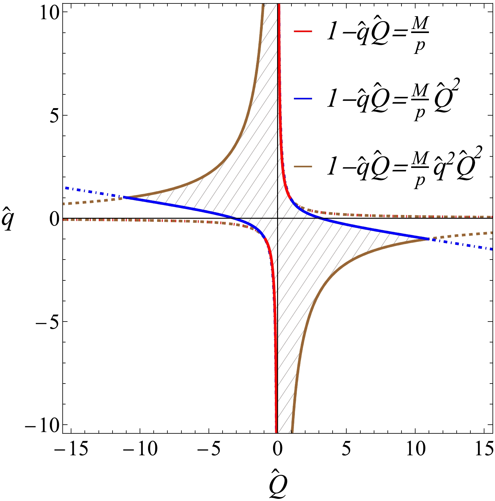

Figure 2

Figure 2.  (color online) Allowed parameter space for PN PS $\alpha_{\rm{RN,PN}}$ to be valid (gray area). The red, blue, and brown boundaries are due to the first, second, and third conditions in Eq. (50), respectively. We fix $p=10M$ in this plot to separate the curves visually. A more relativistic value of p will only change this figure quantitatively.

DownLoad: Full-Size Img PowerPoint

In the following analysis, we examine the influence of variables $\hat q$ and $\hat Q$ on the PS. We focus on the leading order(s) of $M/p$. When $\hat q\hat Q\ll 1$, we can expand the denominator of Eq. (48), and the PS to order $(\hat{q}\hat{Q})^2$ becomes

When $\hat q\hat Q=0$, the electrostatic effect no longer exists, and the Schwarzschild result to the leading order is recovered. For fixed nonzero $\hat Q$ and $0<|\hat q\hat Q|\ll 1$, the first order term $(\hat q\hat Q)^1\hat Q^2$ dominates the second order $(\hat q\hat Q)^2$ term. Comparing to neutral particles, we observe that a small electrostatic attractive (or repulsive) force due to small $|\hat q|$ with ${\rm{sign}}(\hat q\hat Q)=-1$ (or ${\rm{sign}}(\hat q\hat Q)= +1$) increases (or decreases) the PS, similar to the effect of larger (or smaller) M to the PS of neutral particles in Schwarzschild spacetime. However, when $|\hat q|$ exceeds $|\hat Q|/2$, Eq. (51) indicates that the $\hat q^2\hat Q^2$ term becomes larger than $\hat q\hat Q^3$ and, therefore, the PS will increase as $|\hat q|$ increases. In Fig. 3, we plot the dependence of the PS on $\hat q$ for three typical $\hat Q$ values ($\hat Q=$1/10, 1/5, 2/5) using the red curves. For very small $\hat Q$, the dependence is visually suppressed by the largeness of the PS at large$\hat q$ and $\hat Q$. If we fix $\hat q$ as nonzero and vary $\hat Q$ to but still maintain $0<|\hat q\hat Q|\ll 1$, as $\hat Q$ deviates from zero, the PS (51) to the leading orders of $\hat Q$ will behave as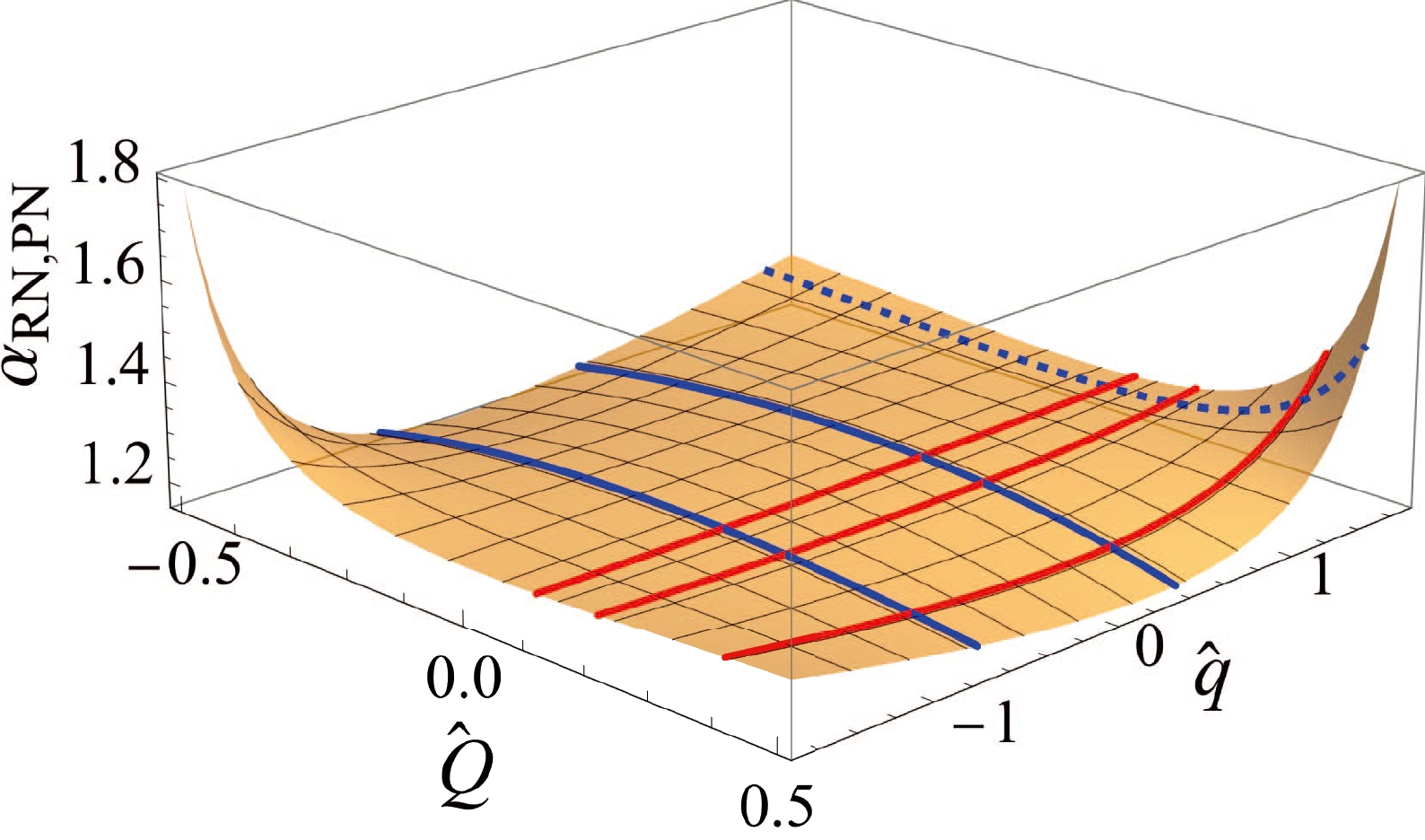

Figure 3

Figure 3.  (color online) Dependence of $\alpha_{\rm{RN,PN}}$ for small $\hat q\hat Q$. The red curves correspond to $\hat Q=1/10,\,1/5,\,2/5$ and the solid and dashed blue curves correspond to $\hat{q}=-7/10,2/5$ and $\hat{q}=3/2$, respectively. We select $p=20M,\; e=4/5,\; |\hat{Q}|<2/5,\;$$|\hat{q}|<5/3$ for the qualitative features to be visible.

DownLoad: Full-Size Img PowerPoint

This means that, in this region, the increase in $\hat Q$ decreases (or increases) the PS if $|\hat q|$ is smaller (or larger) than 1. This dependence on $\hat Q$ is shown by the blue curves in Fig. 3.

In Fig. 4, we plot the orbits for several choices of $\hat q$ and $\hat Q$ to illustrate the dependence of the PS on them. The starting points of these orbits are all set at the positive x-axis, which are also their apoapses. We observe that the PS decreases first and then increases as $\hat q$ increases for fixed $\hat Q$. For fixed $|\hat q|<1$ (or $|\hat q|>1$), it decreases (or increases) as $|\hat Q|$ increases. These agree perfectly with the analysis above.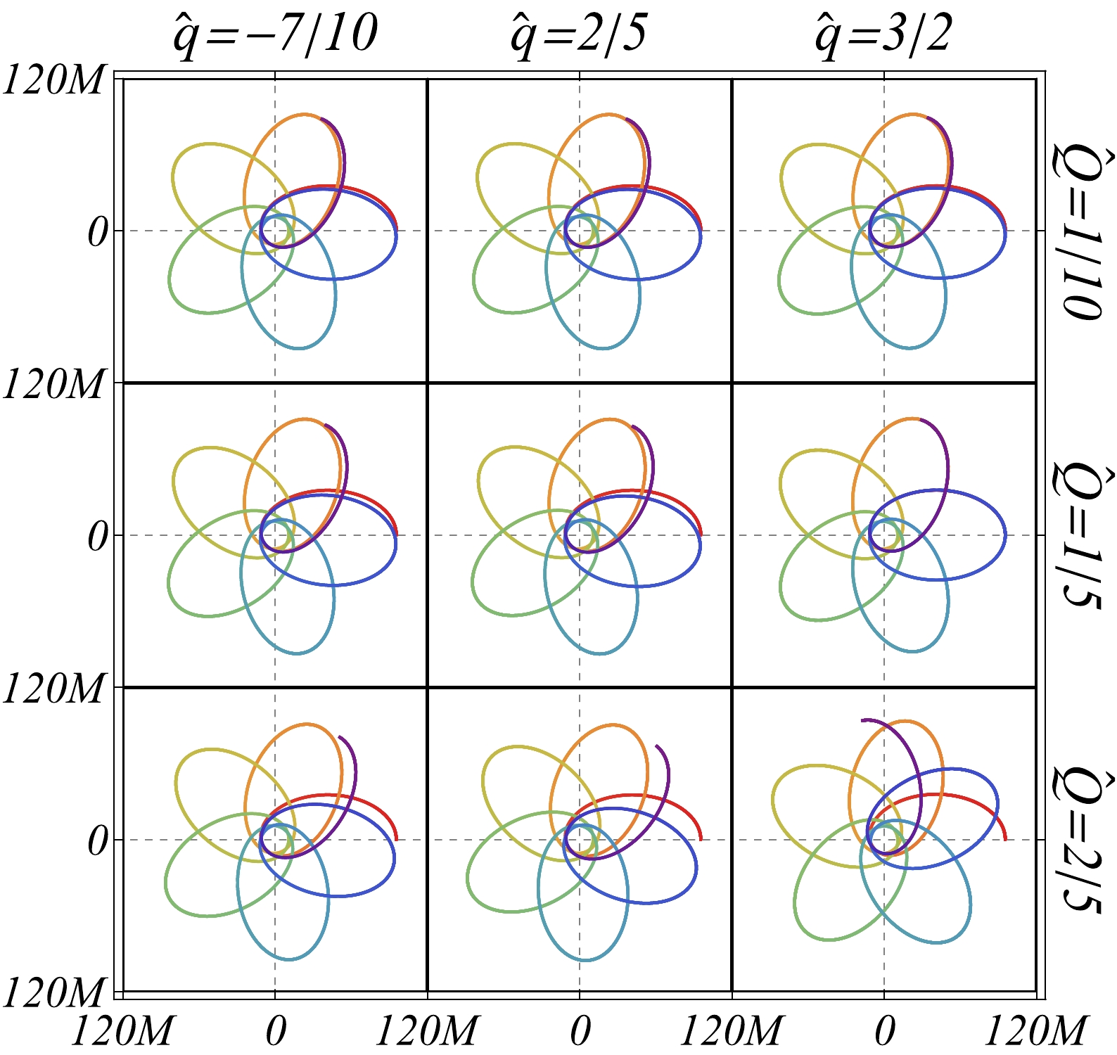

Figure 4

Figure 4.  (color online) Orbits and their PSs of charged test particles in RN spacetime. The corresponding $\hat q$ and $\hat Q$ are shown on top and right side of the plots. We select $p=20M,$$e=4/5$ for the PS to be distinguishable by eye.

DownLoad: Full-Size Img PowerPoint

B PS in EMD gravity

• I. INTRODUCTION
• II. PRELIMINARIES AND THE NC APPROXIMATION
• III. PS USING THE PN METHOD
• IV. APPLICATIONS TO CHARGED SPACETIMES
•      A PS in RN spacetime
•      B PS in EMD gravity
•      C PS in charged wormhole spacetime
• V. CONSTRAINT ON CHARGES OF KNOWN SYSTEMS
•      A Constraints on solar and Mercury charges
•      B Constraints on Sgr A$^{*}$ and S2 charges
• VI. CONCLUSIONS AND DISCUSSION
• ACKNOWLEDGMENTS
• APPENDIX A: PS IN OTHER SPHERICAL SPACETIMES
•      1 PS with Einstein–Maxwell-scalar field
•      2 PS in charged Horndeski spacetime
•      3 PS in charged black-bounce RN spacetimes

The EMD theory is a captivating theoretical framework that combines general relativity, electromagnetism, and the dilaton field minimally, providing a useful starting point for unifying all the fundamental interactions. For the static and spherical solution in this theory, its line element and electric field are described by [32, 33]

where $r_\pm$ represents the locations of the outer and inner event horizons, respectively, $\eta_1=\pm1$ depending on the dilaton/antidilaton nature of the scalar field, and λ is the real (anti)dilaton-Maxwell coupling constant. These parameters can be linked to the mass and charge of the spacetime by

or equivalently

Here, $\eta_2=\pm1$ for Maxwell and anti-Maxwell fields, respectively. When $\gamma=\eta_2=1$, metric (53a) reduces to the normal RN spacetime.

Substituting the asymptotic expansion coefficients of the metric and the electric potential functions in Eq. (53a) into Eq. (40), we determine the PS of charged test objects in the PN approximation in the EMD gravity to the leading order of $1/p$ as

The Maxwell-gravity coupling constant $\eta_2$ also determines the sign of its contribution to the PS through gravity (the $\eta_2\hat{Q}^2$ term). This sign choice also affects the PS through the electric interaction term proportional to $\hat{q}\hat{Q}$, but only weakly when $\hat{Q}$ is small. Parameter γ, which is related to the strength λ of the Maxwell-(anti-)dilaton coupling, determines the amount of deviation of the electric interaction from the standard RN case. In limits $\eta_2=\gamma=1$, this PS agrees with that of the RN case in Eq. (48).

We observe that, by inspecting the higher order terms of the PS (56), the coefficient of order $1/p^{-n}$ contains a factor of $\eta_2\left(1+\gamma\right)$ up to order $- {n}/{2}$. Therefore, for the total PS to converge, condition $p>1/\sqrt{|1+\gamma|}$ should be fulfilled. In Fig. 5, we show the effect of Maxwell-(anti)dilaton parameter γ on the PS for different signs of $\hat{q}$ and $\eta_2$, with all other continuous parameters fixed. For the region of γ, we observe that the PSs are well defined for both $\eta_2$ values, and the effects of γ are always opposite for different $\eta_2$ and signs of $\hat q$. Near the location of $\gamma=1$, the PS decreases (or increases) as γ increases for normal Maxwell field, i.e., $\eta_2=+1$ (or anti-Maxwell field i.e. $\eta_2=-1$), for positive $\hat q$. This means that stronger Maxwell-dilaton coupling will result in a smaller (or larger) PS if the electromagnetic field is Maxwell (or anti-Maxwell) for positive particle charges. In comparison, the effect of γ when $\gamma\lesssim 2$ is the opposite to its effect when $\gamma\gtrsim 1$. When $|\gamma|\gg 1$, then its effect on the PS diminishes as $|\gamma|$ increases, as shown by Eq. (56).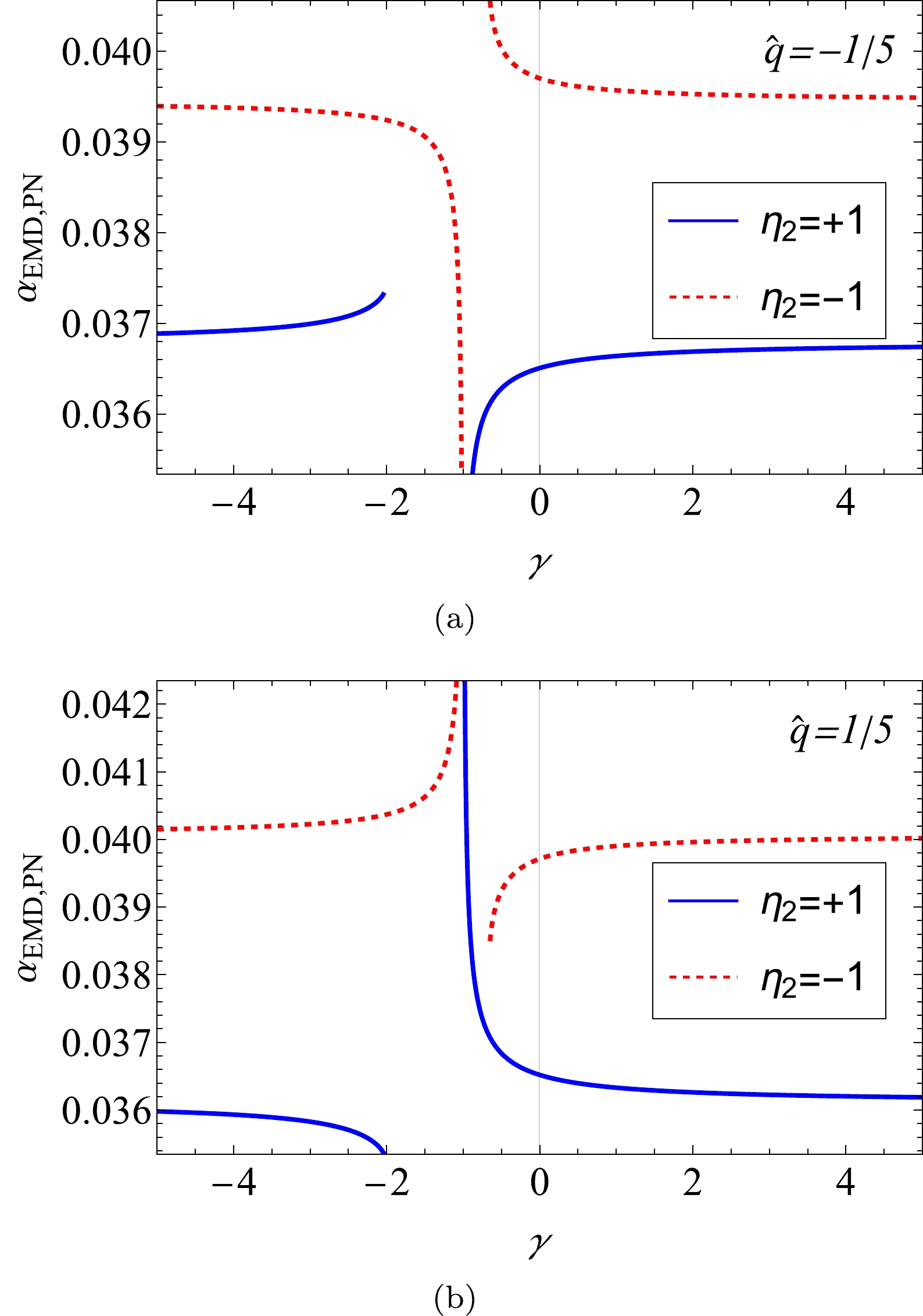

Figure 5

Figure 5.  (color online) Dependence of $\alpha_{\rm{EMD,PN}}$ on γ with $p=500M,\; e=1/10,\; \hat{Q}=1/2,\; \hat{q}=\pm 1/5$. For $r_+,\; r_-$ in Eq. (55) to exist, we require $\gamma<-2$ for $\eta_2=+1$ and $\gamma>-2/3$ for $\eta_2=-1$. The blue and red curves correspond to $\eta_2=+1$ and $\eta_2=-1$, respectively.

DownLoad: Full-Size Img PowerPoint

C PS in charged wormhole spacetime

• I. INTRODUCTION
• II. PRELIMINARIES AND THE NC APPROXIMATION
• III. PS USING THE PN METHOD
• IV. APPLICATIONS TO CHARGED SPACETIMES
•      A PS in RN spacetime
•      B PS in EMD gravity
•      C PS in charged wormhole spacetime
• V. CONSTRAINT ON CHARGES OF KNOWN SYSTEMS
•      A Constraints on solar and Mercury charges
•      B Constraints on Sgr A$^{*}$ and S2 charges
• VI. CONCLUSIONS AND DISCUSSION
• ACKNOWLEDGMENTS
• APPENDIX A: PS IN OTHER SPHERICAL SPACETIMES
•      1 PS with Einstein–Maxwell-scalar field
•      2 PS in charged Horndeski spacetime
•      3 PS in charged black-bounce RN spacetimes

A Lorentzian traversable wormhole with a charge is described by the line element (1) with metric functions and field strength [34]:

where $s(r)$ is the shape function,

and $\beta<-1/2$. For the PN method to be effective, exponent $\dfrac{2\beta}{2\beta+1}$ must be an integer. Therefore, we fix $\beta=-1$ and, consequently, $s(r)=s_0^2/r$. This implies that $s_0$ plays the role of an additional charge, although only partially, through the metric function $B(r)$. Parameter $s_0$ in this spacetime must satisfy $s_0^2>Q^2$ to maintain the wormhole.

The asymptotic form of the metric functions (57b) can be obtained easily. For potential ${\cal{A}}_0$, we can obtain its asymptotic expansion by expanding and then integrating (57d):

Substituting these expansions into Eq. (40), the PS in this charged wormhole spacetime becomes

When $s_0$ is set to zero, this agrees with the PS (48) in the RN case with $M=0$. Therefore, the PS in this spacetime can be considered as that of a massless RN spacetime with some modifications from parameter $s_0$. Moreover, the fundamental scale in this spacetime can be selected as the charge Q.

Among the two terms in the leading order, the term proportional to $Q/\hat{q}$ is due to the gravitational effect of the spacetime charge, whereas the term proportional to $-\hat{q}Q$ is still caused by the electric interaction. The extra parameter $s_0$ only appears starting from the $(Q/p)^2$ order and affects the PS only through gravitation (no multiplication with $\hat{q}$). This also agrees with the fact that $s_0$ does not appear in the leading order of the electric potential in Eq. (59). Similar to the previous analysis after Eq. (48) for the convergence requirement in the RN spacetime, the $\alpha_{{\rm{CW,PN}}}$ here also consists of four distinct series and the convergence of the PS requires

Additionally, differentiating Eq. (3c) with respect to τ again, we find that, in this spacetime,

Because $Q^2+r^2-s_0^2>0$ due to $B(r)>0$ in the observable region, the above equation shows that if $qQ>0$, $\ddot{r}$ will always be positive, and no bounded orbits or well-defined PS exists. Therefore, we also require that $qQ<0$ in this spacetime to study its PS. This is also consistent with the instinct that when no gravitational attraction exists from the mass ($M=0$), $qQ$ must be negative for the electrostatic interaction to be attractive and form a bound orbit.

In Fig. 6, we plot the dependence of the PS on new parameter $s_0$ (in scale of Q) according to Eq. (60) for a few values of $\hat q$. For all $\hat q$, the PS increases as $s_0/Q$ increases. This is generally consistent with the observation in the RN spacetime in Fig. 3 that as charge $Q^2$ increases, the PS also increases. For each $-1\lesssim\hat q<0$, a value of $s_0/Q$ below which the PS becomes negative exists. However, this characteristic is not present in the regular RN case because the PS is mostly positive for reasonable parameter choices. This critical value of $s_0$ can also be solved from Eq. (60) to the leading two orders as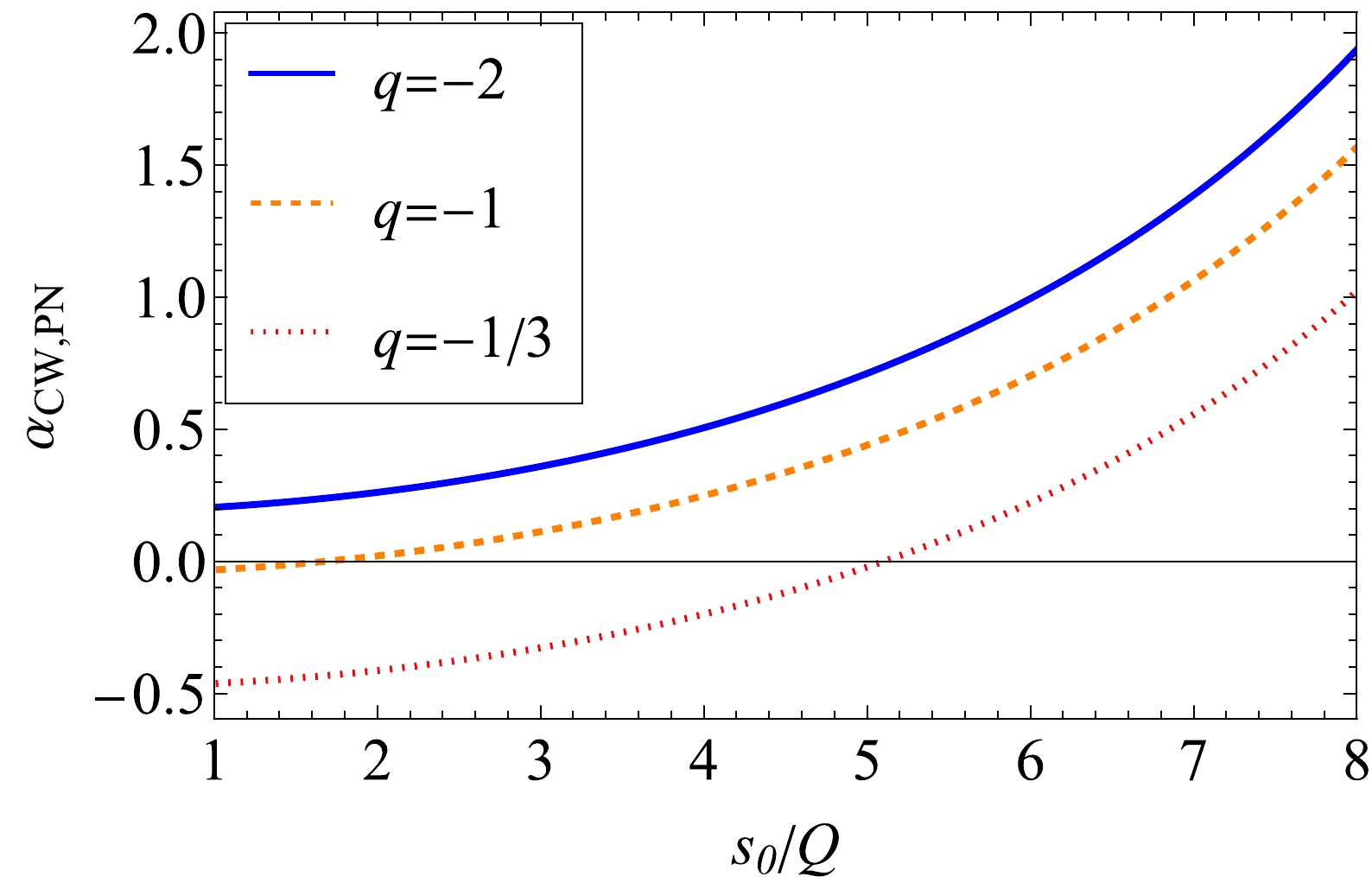

Figure 6

Figure 6.  (color online) Dependence of $\alpha_{\rm{CW,PN}}$ on $s_0$ with fixed $Q=1,\; p=20Q,\; e=1/2$.

DownLoad: Full-Size Img PowerPoint

From this, we observe that for positive Q, because $qQ$ must be negative, the existence of such critical $s_0$ requires that $1\lesssim\hat q<0$, which is consistent with the observations in Fig. 6.

In Fig. 7, we use $\hat q=-1/3$, which corresponds to the red dotted curve in Fig. 6, and three typical values of $s_0/Q\; (2, 7, 8)$ to plot the corresponding orbits. The first of these according to Fig. 6 corresponds to the orbit with a negative PS, whereas the latter two have positive PSs. Fig. 7 verifies this, and we have checked that the PS in these orbits agrees quantitatively with the value in Fig. 6 and Eq. (60).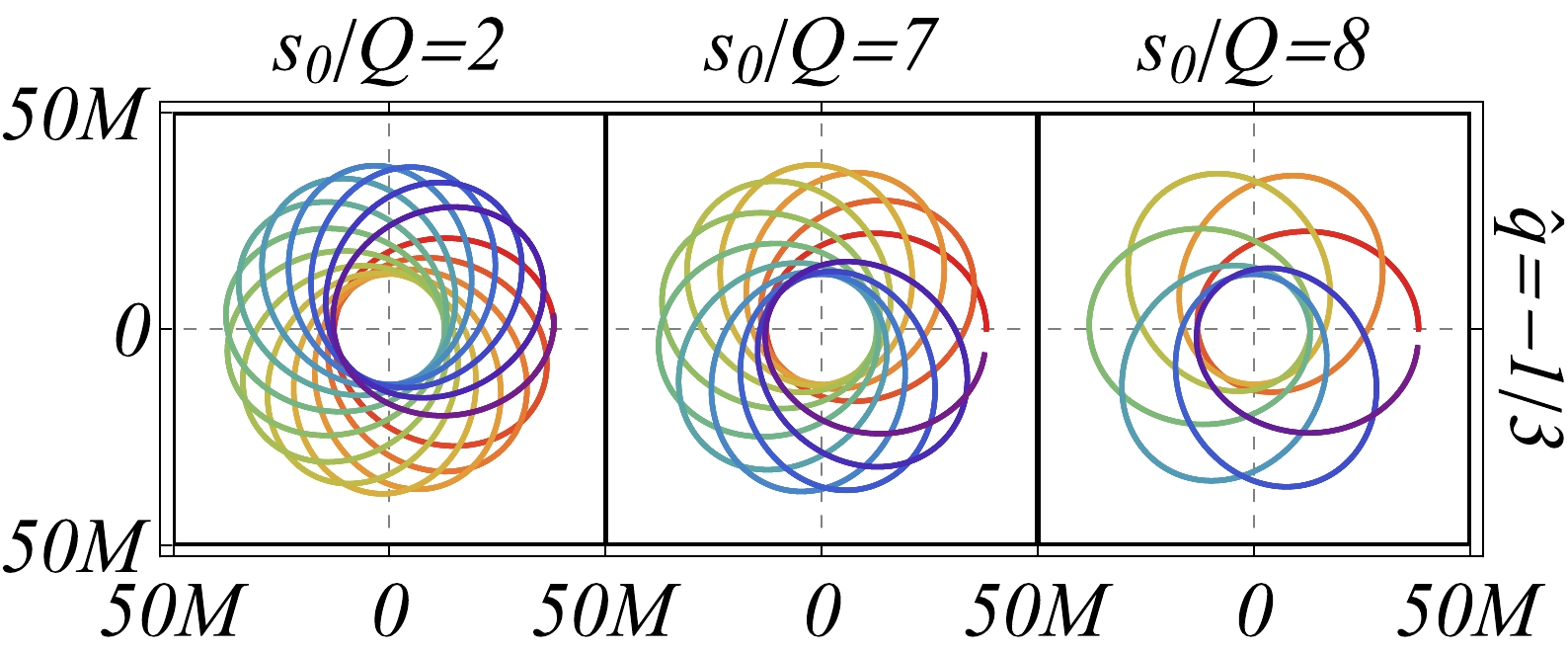

Figure 7

Figure 7.  (color online) Orbits of charged test particles in the charged wormhole. We use $Q=1,\; \hat q=-1/3,\; p=20Q,\; e=1/2$ and three $s_0/Q$ as indicated in the plot.

DownLoad: Full-Size Img PowerPoint

V. CONSTRAINT ON CHARGES OF KNOWN SYSTEMS

• I. INTRODUCTION
• II. PRELIMINARIES AND THE NC APPROXIMATION
• III. PS USING THE PN METHOD
• IV. APPLICATIONS TO CHARGED SPACETIMES
•      A PS in RN spacetime
•      B PS in EMD gravity
•      C PS in charged wormhole spacetime
• V. CONSTRAINT ON CHARGES OF KNOWN SYSTEMS
•      A Constraints on solar and Mercury charges
•      B Constraints on Sgr A$^{*}$ and S2 charges
• VI. CONCLUSIONS AND DISCUSSION
• ACKNOWLEDGMENTS
• APPENDIX A: PS IN OTHER SPHERICAL SPACETIMES
•      1 PS with Einstein–Maxwell-scalar field
•      2 PS in charged Horndeski spacetime
•      3 PS in charged black-bounce RN spacetimes

In this section, we apply the PS in the RN spacetime to the observed PS of Mercury around the Sun and S2 around Sgr A^* to constrain the charges of these objects.

A Constraints on solar and Mercury charges

• I. INTRODUCTION
• II. PRELIMINARIES AND THE NC APPROXIMATION
• III. PS USING THE PN METHOD
• IV. APPLICATIONS TO CHARGED SPACETIMES
•      A PS in RN spacetime
•      B PS in EMD gravity
•      C PS in charged wormhole spacetime
• V. CONSTRAINT ON CHARGES OF KNOWN SYSTEMS
•      A Constraints on solar and Mercury charges
•      B Constraints on Sgr A$^{*}$ and S2 charges
• VI. CONCLUSIONS AND DISCUSSION
• ACKNOWLEDGMENTS
• APPENDIX A: PS IN OTHER SPHERICAL SPACETIMES
•      1 PS with Einstein–Maxwell-scalar field
•      2 PS in charged Horndeski spacetime
•      3 PS in charged black-bounce RN spacetimes

The MESSENGER spacecraft measured an uncertainty of $9\times 10^{-4}\; ''/$cty for the Schwarzschild-like precession of Mercury around the Sun [35]. If we associate this uncertainty to the electric effect of solar charge $\hat Q_\odot$ and Mercury charge $\hat q$_☿, then this uncertainty can be used to constrain the charges in the parameter space spanned by them. The result is shown in Fig. 8, where the allowed region of $\hat q$_☿ and $\hat Q_\odot$ are enclosed by four segments of blue boundaries and two vertical red boundaries. The blue boundaries are due to the leading order of Eq. (48) because, in this case, p_☿/$M_{\odot}=3.8\times 10^7$, which makes the first order sufficient for the estimation of the PS. In other words, we treat this uncertainty as

Figure 8

Figure 8.  (color online) Allowed parameter space of $\hat{q}$_☿ and $\hat Q_{\odot}$. $M_\odot=1.988\times 10^{30}\; {\rm{kg}}$, M_☿ = $3.301\times 10^{23}{\rm{kg}}$ [37], $e=0.2056$, $p=5.545\times 10^{10}\; {\rm{m}}$ [35] for Mercury are used.

DownLoad: Full-Size Img PowerPoint

where, in the last term of the first line, we deduce the Schwarzschild contribution. Therefore, we observe that these blue boundaries are oddly symmetric, meaning that the change of signs $(\hat q\to-\hat q,\,\hat Q\to -\hat Q)$ will not change the extra PS. Moreover, we observe that these boundaries are generally not evenly symmetric, i.e., when only one charge changes sign, the value of $\Delta\alpha$ changes. However, in the current case, since the extra PS is very small, the total value of the allowed $\hat q\hat Q$ is already very small, and this nonsymmetry cannot be recognized in the plot using bare eyes. The red boundaries on the solar charge at two ends of $\hat Q_\odot$ are obtained from the tight constraint in Ref. [36].

The constrained value of the solar charge is much tighter than the previously reported value using the PS data, if we assume the same charge for Mercury (see Eqs. (42) and (43) of Ref. [24]).

B Constraints on Sgr A$^{*}$ and S2 charges

• I. INTRODUCTION
• II. PRELIMINARIES AND THE NC APPROXIMATION
• III. PS USING THE PN METHOD
• IV. APPLICATIONS TO CHARGED SPACETIMES
•      A PS in RN spacetime
•      B PS in EMD gravity
•      C PS in charged wormhole spacetime
• V. CONSTRAINT ON CHARGES OF KNOWN SYSTEMS
•      A Constraints on solar and Mercury charges
•      B Constraints on Sgr A$^{*}$ and S2 charges
• VI. CONCLUSIONS AND DISCUSSION
• ACKNOWLEDGMENTS
• APPENDIX A: PS IN OTHER SPHERICAL SPACETIMES
•      1 PS with Einstein–Maxwell-scalar field
•      2 PS in charged Horndeski spacetime
•      3 PS in charged black-bounce RN spacetimes

The precession of S2 around Srg A$^{*}$ was measured recently by the Gravity group [9] to yield ratio f of the measured value to the standard Schwarschild-precession. A value of $f=1.10\pm 0.19$ was obtained. If we associate the deviation of the central value from 1 to the electric effect of the Sgr A^* and S2 charges, then similar to the Mercury precession, we can use this deviation to determine the allowed region in the parameter space of $\hat q_{\rm{S2}}$ and $\hat Q_{\rm{Sgr\ A}^*}$.

The result is shown in Fig. 9, where the blue boundaries indicate the leading order of Eq. (48). In this case, $p/M_{\rm{Sgr\ A}^*}=5\times 10^3$ [40] is sufficiently large such that the first order of the PS is sufficient for estimating $\hat q_{\rm{S2}}$ and $\hat Q_{\rm{Sgr\ A}^*}$. In this allowed parameter space, because the maximal $\hat q\hat Q$ value can be as large as $0.8$, from Eq. (64) and comparing to the plot in Fig. 8, its nonsymmetry under sign change $(\hat q\to-\hat q,\,\hat Q\to\hat Q)$ or $(\hat q\to\hat q,\,\hat Q\to-\hat Q)$ is very clear. The red boundary on the Sgr A^* charge is due to the constraint from the shadow size of the Sgr A^* [41] (see [42–44] for other bounds on this charge). To our best knowledge, the allowed region in Fig. 9 is the first combined constraint on charge $\hat q_{\rm{S2}}$ and $\hat Q_{\rm{Sgr\ A}^*}$ using the S2 PS data.

Figure 9

Figure 9.  (color online) Allowed regions of $\hat{q}_{\rm{S2}}$ and $\hat Q_{\rm{Sgr\ A}^*}$. $M_{\rm{Sgr\ A}^*}=4.15\times 10^6 M_{\odot}$ [38], $M_{\rm S2}=13.6M_{\odot}$ [39], $e=0.8843,\;$$p=3.336\times 10^{13}{\rm{m}}$ [40] are used.

DownLoad: Full-Size Img PowerPoint

VI. CONCLUSIONS AND DISCUSSION

• I. INTRODUCTION
• II. PRELIMINARIES AND THE NC APPROXIMATION
• III. PS USING THE PN METHOD
• IV. APPLICATIONS TO CHARGED SPACETIMES
•      A PS in RN spacetime
•      B PS in EMD gravity
•      C PS in charged wormhole spacetime
• V. CONSTRAINT ON CHARGES OF KNOWN SYSTEMS
•      A Constraints on solar and Mercury charges
•      B Constraints on Sgr A$^{*}$ and S2 charges
• VI. CONCLUSIONS AND DISCUSSION
• ACKNOWLEDGMENTS
• APPENDIX A: PS IN OTHER SPHERICAL SPACETIMES
•      1 PS with Einstein–Maxwell-scalar field
•      2 PS in charged Horndeski spacetime
•      3 PS in charged black-bounce RN spacetimes

In this paper, we employ two methods, NC and PN approximations, to systematically study the effect of both gravitational and electrostatic interaction on the PS of charged test particles in general static and spherically symmetric charged spacetimes. The PSs using both methods are determined to high orders and are numerically verified to be very accurate as long as the truncation order is sufficiently high. The NC PS is shown to be more effective when the eccentricity is smaller, whereas the PN result is more accurate when the semilatus rectum is large. These results are shown to be equivalent when e is small and p is large.

The methods are then applied to the RN, EMD, and charged wormhole spacetimes. Generally, the PS exists only for certain regions in the parameter space spanned by the spacetime charge Q and particle charge q. Generally, condition $qQ<mM$ is always necessary for the electrostatic interaction to be weaker than the gravitational attraction if it is repulsive. Spacetime charge Q is observed to influence the PS through both the gravitational and electrostatic channels. The combined effect is that the PS decreases (or increases) if $|\hat q|<1$ (or $|\hat q|>1$) as $|\hat Q|$ deviates from zero.

The solar-Mercury and Sgr A^*-S2 systems are then modeled using the RN spacetime, and their PS data are used to constrain the charge of these objects. For both systems, we determined the allowed regions of these charges in the $(\hat q,\,\hat Q)$ parameter space. For the Sgr A^*-S2 system, as far as we know, this is the first time that such a constraint is made using the PS data.

In Appendix A, we present the PS determined using the PN method in three other charged spacetimes, the Einstein-Maxwell-scalar gravity and charged Horndeski and charged black-bounce RN spacetimes. They are not given in the main text because to the first order, their PS (almost) coincide with the RN result and therefore is expected to be non-distinguishable from the RN one using currently available data.

Although the effect of the electrostatic interaction on the PS in spherically symmetric spacetime is generallt clear, a few possible extensions remain to be explored. The first is to investigate the effect of a magnetic field on the PS because the magnetic field is (even more) commonly considered to exist in interstellar space. The second is that we can study the effect of other properties of the test particle on the PS, such as when the particle itself is spinning. We are currently pursuing some of these directions. Finally, we also acknowledge the recent studies using the Gauss-Bonnet theorem method for the deflection angle of bound and overlapping orbits [45, 46]. This interesting development could potentially be used to compute the PS too.

ACKNOWLEDGMENTS

• I. INTRODUCTION
• II. PRELIMINARIES AND THE NC APPROXIMATION
• III. PS USING THE PN METHOD
• IV. APPLICATIONS TO CHARGED SPACETIMES
•      A PS in RN spacetime
•      B PS in EMD gravity
•      C PS in charged wormhole spacetime
• V. CONSTRAINT ON CHARGES OF KNOWN SYSTEMS
•      A Constraints on solar and Mercury charges
•      B Constraints on Sgr A$^{*}$ and S2 charges
• VI. CONCLUSIONS AND DISCUSSION
• ACKNOWLEDGMENTS
• APPENDIX A: PS IN OTHER SPHERICAL SPACETIMES
•      1 PS with Einstein–Maxwell-scalar field
•      2 PS in charged Horndeski spacetime
•      3 PS in charged black-bounce RN spacetimes

The authors appreciate the discussion with S. Xu and J. He.

APPENDIX A: PS IN OTHER SPHERICAL SPACETIMES

• I. INTRODUCTION
• II. PRELIMINARIES AND THE NC APPROXIMATION
• III. PS USING THE PN METHOD
• IV. APPLICATIONS TO CHARGED SPACETIMES
•      A PS in RN spacetime
•      B PS in EMD gravity
•      C PS in charged wormhole spacetime
• V. CONSTRAINT ON CHARGES OF KNOWN SYSTEMS
•      A Constraints on solar and Mercury charges
•      B Constraints on Sgr A$^{*}$ and S2 charges
• VI. CONCLUSIONS AND DISCUSSION
• ACKNOWLEDGMENTS
• APPENDIX A: PS IN OTHER SPHERICAL SPACETIMES
•      1 PS with Einstein–Maxwell-scalar field
•      2 PS in charged Horndeski spacetime
•      3 PS in charged black-bounce RN spacetimes

1 PS with Einstein–Maxwell-scalar field

• I. INTRODUCTION
• II. PRELIMINARIES AND THE NC APPROXIMATION
• III. PS USING THE PN METHOD
• IV. APPLICATIONS TO CHARGED SPACETIMES
•      A PS in RN spacetime
•      B PS in EMD gravity
•      C PS in charged wormhole spacetime
• V. CONSTRAINT ON CHARGES OF KNOWN SYSTEMS
•      A Constraints on solar and Mercury charges
•      B Constraints on Sgr A$^{*}$ and S2 charges
• VI. CONCLUSIONS AND DISCUSSION
• ACKNOWLEDGMENTS
• APPENDIX A: PS IN OTHER SPHERICAL SPACETIMES
•      1 PS with Einstein–Maxwell-scalar field
•      2 PS in charged Horndeski spacetime
•      3 PS in charged black-bounce RN spacetimes

For a minimally coupled EMS gravity, the spacetime metric and electric field are described by [47]

where $n\in(1/2,1]$, and

are the location of the outer and inner event horizons, and n is related to the scalar charge.

Substituting the asymptotics of these functions into Eq. (40), the PS in the EMS field in the PN approximation is found as

To the leading order, this agrees with the RN result (48). Therefore, distinguishing this spacetime from the RN one using the current observation data would be difficult.

2 PS in charged Horndeski spacetime

• I. INTRODUCTION
• II. PRELIMINARIES AND THE NC APPROXIMATION
• III. PS USING THE PN METHOD
• IV. APPLICATIONS TO CHARGED SPACETIMES
•      A PS in RN spacetime
•      B PS in EMD gravity
•      C PS in charged wormhole spacetime
• V. CONSTRAINT ON CHARGES OF KNOWN SYSTEMS
•      A Constraints on solar and Mercury charges
•      B Constraints on Sgr A$^{*}$ and S2 charges
• VI. CONCLUSIONS AND DISCUSSION
• ACKNOWLEDGMENTS
• APPENDIX A: PS IN OTHER SPHERICAL SPACETIMES
•      1 PS with Einstein–Maxwell-scalar field
•      2 PS in charged Horndeski spacetime
•      3 PS in charged black-bounce RN spacetimes

The charged Horndeski spacetime is described by the metric and potential functions [48, 49]:

The expansion of these functions are easy. Subsequently, substituting this into Eq. (40), the PN PS in this spacetime is determined as

To the leading order, this is different from the RN result in the gravitational contribution of $\hat{Q}$ by a factor of a quarter.

3 PS in charged black-bounce RN spacetimes

• I. INTRODUCTION
• II. PRELIMINARIES AND THE NC APPROXIMATION
• III. PS USING THE PN METHOD
• IV. APPLICATIONS TO CHARGED SPACETIMES
•      A PS in RN spacetime
•      B PS in EMD gravity
•      C PS in charged wormhole spacetime
• V. CONSTRAINT ON CHARGES OF KNOWN SYSTEMS
•      A Constraints on solar and Mercury charges
•      B Constraints on Sgr A$^{*}$ and S2 charges
• VI. CONCLUSIONS AND DISCUSSION
• ACKNOWLEDGMENTS
• APPENDIX A: PS IN OTHER SPHERICAL SPACETIMES
•      1 PS with Einstein–Maxwell-scalar field
•      2 PS in charged Horndeski spacetime
•      3 PS in charged black-bounce RN spacetimes

The charge black-bounce RN spacetime is described by the RN metric functions with r replaced by $\sqrt{r^2+l^2}$, where l is a length scale (usually associated with the Planck length), i.e., the new metric functions. The electric potential becomes [50]

The asymptotic expansions of these functions are also simple, and after substituting the coefficients into Eq. (40), we can directly obtain the PS in this spacetime. To the second order, this is

where the $\alpha_{{\rm{RN,PN}}}$ is the PS of the RN spacetime in Eq. (48). The extra scale parameter l only appears from the second order of $1/p$; therefore, the PS in this spacetime is also difficult to distinguish from that in the regular RN spacetime. Moreover, to the ${\cal{O}}(M/p)^2$ order, the scale parameter l does not participate in any electric interaction effect to the PS. We also checked that this will change beginning from the ${\cal{O}}(M/p)^3$ order, i.e., terms proportional to $l^2\hat q\hat Q$ and $l^2\hat q^2\hat Q^2$ exist in the PS at this order. The result (A7), after setting $\hat q=0$, reduces to the PS of neutral particles in black-bounce RN spacetime [23].

References