-
The cosmic distance duality relation (DDR), also known as the Etherington relation [1], plays a fundamental role in modern cosmology. This relation connects two critical measurements of cosmic distance for an astronomical object: luminosity distance
$ D_L $ and angular-diameter distance$ D_A $ . In a spacetime described by a metric theory of gravity, where the number of photons is conserved as they travel along null geodesics, DDR can be formulated as$ D_A(z)(1+z)^2/D_L(z) = 1 $ , with z representing the redshift of the astronomical object. Any deviation from the standard DDR may imply the presence of new physics. Various phenomena can lead to the violation of DDR, such as photons coupling with non-standard particles [2], dust extinction [3], variations in fundamental constants [4], and systematic observational errors [5]. Moreover, as a cornerstone relation in cosmology, the DDR has been extensively employed to probe gas-mass density profiles [6], determine the shapes of galaxy clusters [7], and constrain cosmological parameters [8, 9]. Therefore, verifying the validity of DDR is crucial.A variety of methodologies, both cosmological model-dependent and model-independent, have been employed to probe DDR. Model-dependent approaches evaluate DDR under specific cosmological model assumptions [10−14], whereas model-independent methods are generally affected by large uncertainties [15−19]. Testing DDR typically involves two distinct distance measurements: luminosity distance and angular-diameter distance. The most straightforward comparison entails evaluating these two distances at the same redshift. However, the simultaneous measurement of luminosity and angular-diameter distances for a single astronomical object poses significant challenges, necessitating their derivation from disparate observations. Such observations may include Type Ia supernovae (SNe Ia), gamma-ray bursts (GRBs),
$ H(z) $ measurements, angular-diameter distances of galaxy clusters, galaxy-cluster gas mass fractions, Einstein radii of strong gravitational lenses (SGLs), and gravitational waves, among others. To reconcile these measurements at a common redshift, several methodologies have been proposed, including the nearby SNe Ia method to match redshifts [16, 18], Gaussian process (GP) techniques [20, 21], and artificial neural network (ANN) approaches [22, 23], for reconstructing the distance-redshift relation.Among the various approaches proposed for testing DDR, SNe Ia have emerged as the most frequently utilized. For example, Li et al. [16] employed the nearby SNe Ia method, combining the Union2 SNe Ia sample with two galaxy cluster samples. They assessed DDR at 1σ confidence level with 18 galaxy clusters, and at 2σ confidence level with 38 galaxy clusters. Liao et al. [18] combined the SGL systems with the JLA SNe Ia compilation, and confirmed the validity of DDR at 1σ confidence level. Similarly, Zhou et al. [19] verified DDR using the Pantheon SNe Ia sample and SGL systems, achieving 1σ confidence level. Employing the GP method to reconstruct the distance-redshift relation from the Pantheon dataset, Lin et al. [24] corroborated the validity of DDR at 1σ confidence level using two galaxy cluster samples. Liu et al. [23] compared the precision of DDR tests using data reconstructed by GP and ANN methods, and revealed that the GP method provides higher precision (10−3 level) compared to the ANN method (10−2 level).
The integration of refined astrophysical datasets and forthcoming observational advancements aims to enhance the precision of DDR testing [25−30]. Recently, Scolnic et al. [31] presented the Pantheon+ dataset, a comprehensive and meticulously curated compilation that substantially expands the catalog of SNe Ia light curves available for cosmological studies. The Pantheon+ dataset encompasses 1701 light curves from 1550 spectroscopically confirmed SNe Ia. The cross-calibration of photometric systems within the Pantheon+ sample, along with the subsequent re-calibration of the SALT2 light-curve model [32], significantly reduces the systematic uncertainties and enhances the accuracy of distance modulus measurements. Additionally, the
$ H_0 $ Lenses in COSMOGRAIL's Wellspring (H0LiCOW) collaboration has provided six gravitationally lensed quasars with precisely measured time-delay distances [33−40], constraining the Hubble constant$ H_0 $ to a precision of 2.4% within the standard flat ΛCDM model [41]. From time-delayed gravitational lensing, we can extract the information of angular-diameter distances, thus offering a valuable opportunity to test DDR.In this study, we tested the validity of DDR using the combination of luminosity distances from the Pantheon+ dataset and angular-diameter distances from SGL systems provided by the H0LiCOW. To obtain the luminosity distance at the redshifts of the SGL systems, we employed a GP method to reconstruct the distance-redshift relation from the Pantheon+. The remainder of this paper is structured as follows. Section II details the data and methodology employed in testing DDR. Specifically, Section II.A describes how to measure angular-diameter distances from SGL systems; Section II.B describes the GP reconstruction of the distance-redshift relation from the Pantheon+; and Section II.C shows how to combine the SGL systems and SNe Ia to test DDR. In Section III, we use Monte Carlo simulations to predict the prospects of a larger sample of SGL data in constraining DDR. Finally, Section IV offers a discussion of the findings from this study and draws conclusions based on the conducted analysis.
-
Strong gravitational lensing is a potent tool for exploring the cosmos. When light from a luminous source, such as a quasar, passes near a massive object − the lens − it bends, resulting in observable images of the source. Owing to the different paths light can take, multiple images of the source can appear. The temporal offset between these images is known as the time delay, which can be expressed as [42]
$ \Delta t = \frac{D_{\Delta_t}\Delta\phi({\boldsymbol{\xi}}_{\mathrm{lens}})}{c}, $

(1) where c is the speed of light,
$ \Delta\phi $ represents the Fermat potential difference between the two images, and$ {\boldsymbol{\xi}}_{\mathrm{lens}} $ denotes the parameters of the lens model. The time-delay distance$ D_{\Delta_t} $ is defined by$ D_{\Delta_t} = (1+z_l)\frac{D_A^l D_A^s}{D_A^{ls}}, $

(2) where
$ z_l $ is the redshift of the lens, and$ D_A^l $ ,$ D_A^s $ , and$ D_A^{ls} $ correspond to the angular-diameter distances between the observer and lens, observer and source, and lens and source, respectively. If the time delay is precisely measured and the Fermat potential is well modeled, we can determine the time-delay distance$ D_{\Delta t} $ according to Eq. (1).By incorporating kinematic information from the lens galaxy − such as the light profile
$ {\boldsymbol{\xi}}_{\mathrm{light}} $ , projected stellar velocity dispersion$ \sigma^P $ , and anisotropy distribution of the stellar orbits parameterized by$ \beta_{\mathrm{ani}} $ , the angular-diameter distance from the observer to the lens can be determined by [39]$ D_A^l = \frac{1}{1+z_l}D_{\Delta t}\frac{c^2 {\boldsymbol{J}}({\boldsymbol{\xi}}_{\mathrm{lens}},{\boldsymbol{\xi}}_{\mathrm{light}},\beta_{\mathrm{ani}})}{(\sigma^P)^2}, $

(3) where
$ {\boldsymbol{J}} $ is a function that encapsulates all the model components, derived from angular measurements on the sky and the distribution of stellar orbital anisotropy.According to the Planck 2018 results [43], our universe is spatially flat. In such a flat universe, the angular-diameter distance at redshift z can be expressed in terms of the comoving distance
$ r(z) $ as$ D_A = r(z)/(1+z) $ . The comoving distance between the lens and source is given by$ r^{ls} = r(z_s)-r(z_l) $ , where$ z_l $ and$ z_s $ are the redshifts of lens and source, respectively [44]. Consequently, the angular-diameter distance between the lens and source can be expressed as$ D_A^{ls} = D_A^s-\frac{1+z_l}{1+z_s}D_A^l. $

(4) The COSmological MOnitoring of GRAvItational Lenses (COSMOGRAIL) program [45, 46] is dedicated to the precise measurement of time delays in well-known lensed quasars, utilizing a network of dedicated telescopes located in both the northern and southern hemispheres. Leveraging these time delay measurements alongside detailed models of the mass distribution of the lensing galaxies and their environments, the H0LiCOW collaboration [35] aims to determine the Hubble constant
$ H_0 $ with high precision. Recently, the H0LiCOW collaboration constrained the Hubble constant to an accuracy of 2.4% using a combined sample of six lenses [41]. The posterior distributions for the time-delay distances$ D_{\Delta_t} $ of these six lens systems are available on the H0LiCOW website1 . Additionally, the angular-diameter distances$ D_A^l $ for four of these six lenses, i.e., RXJ1131−1231, PG 1115+80, B1608+656, and SDSS 1206+4332, are also provided.In this study, we only considered the four SGL systems for which both the time-delay and angular-diameter distances to the lens are available. The redshifts and distances of this sample are presented in Table 1. Using the posterior distributions of
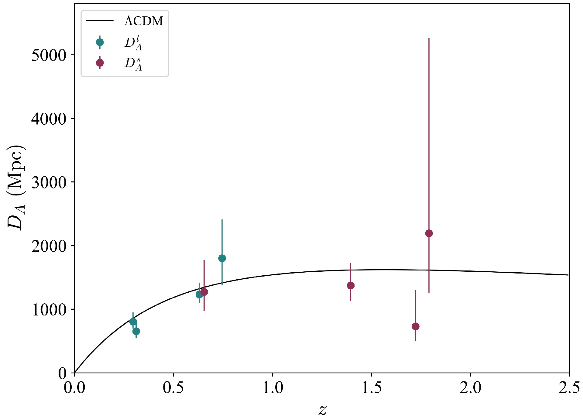
$ D_{\Delta_t} $ and$ D_A^l $ , we can determine the angular-diameter distance to the source$ D_A^s $ by combining Eqs. (2) and (4). For each system, we randomly sampled$ D_{\Delta_t} $ and$ D_A^l $ from their respective posterior distributions 1000 times, and then computed the distribution of$ D_A^s $ . Consequently, our dataset comprises a total of eight angular-diameter distances (one$ D_A^l $ and one$ D_A^s $ for each of the four SGL systems). To illustrate these results, we plot the angular-diameter distances with 1σ uncertainty in Fig. 1. The best-fitting ΛCDM model curve derived from the Pantheon+ dataset is also over-plotted for comparison. Note that most data points are consistent with the ΛCDM curve, regardless of the large uncertainty for some data points. Note that the data points are cosmological model-independent, except for the spatially flat assumption.Lens $ z_l $ 

$ z_s $ 

$ D_{\Delta_t}\ ({\rm{Mpc}}) $ 

$ D_A^l \ ({\rm{Mpc}})$ 

Reference RXJ1131 $ - $ 1231

0.295 0.654 $ 2096_{-83}^{+98} $ 

$ 804_{-112}^{+141} $ 

[34,38] PG 1115+080 0.311 1.722 $ 1470_{-127}^{+137} $ 

$ 697_{-144}^{+186} $ 

[38] B1608+656 0.630 1.394 $ 5156_{-236}^{+296} $ 

$ 1228_{-151}^{+177} $ 

[33,37] SDSS 1206+4332 0.745 1.789 $ 5769_{-471}^{+589} $ 

$ 1805_{-398}^{+555} $ 

[39] Table 1. Redshifts and distances of the SGL sample ordered by lens redshift.
-
SNe Ia are invaluable as distance indicators in cosmological research owing to their nearly constant intrinsic luminosity. The latest Pantheon+ compilation, detailed in Ref. [31], integrates data from 18 distinct surveys, yielding 1701 light curves from 1550 spectroscopically confirmed SNe Ia across a redshift range of
$ z\in[0.001,2.3] $ . According to the modified Tripp relation [47], the observed distance modulus of SNe Ia at redshift z is expressed as$ \mu = m_B-M+\alpha x_1-\beta c_1-\delta_{\mu-\mathrm{bias}}, $

(5) where
$ m_B $ is the apparent magnitude in the B-band and M is the absolute magnitude. The parameters$ x_1 $ and$ c_1 $ represent the stretch and color of the supernovae, respectively. The term$ \delta_{\mu-\mathrm{bias}} $ accounts for the bias correction related to selection effects and other simulation-related issues. Using the BEAMS with bias corrections (BBC) method to calibrate SNe Ia [48], corrected magnitude$ m_{\mathrm{corr}} $ and the corresponding covariance matrix are made available2 . Consequently, Eq. (5) can be simplified to$ \mu = m_{\mathrm{corr}}-M. $

(6) The distance modulus is converted to the luminosity distance using the relation
$ \mu = 5\log_{10}\frac{D_L(z)}{\mathrm{Mpc}}+25. $

(7) To determine the luminosity distance at any redshift, we employed the GP method to reconstruct the distance-redshift relation from the Pantheon+ dataset without any parametric assumptions. The GP method is widely used in cosmological research because of its efficacy in handling regression and classification tasks. To reconstruct a function
$ y = f(x) $ from observational data$ (x_i,y_i) $ , the GP method assumes that the data points are generated from a joint Gaussian distribution:$ {\boldsymbol{y}}\sim {\cal{N}}({\boldsymbol{\mu}},{\bf{K}}({\boldsymbol{x}},{\boldsymbol{x}})+{\bf{C}}), $

(8) where
$ {\boldsymbol{x}} = \{x_i\} $ ,$ {\boldsymbol{y}} = \{y_i\} $ are the observational vectors,$ \boldsymbol\mu $ is the mean of the Gaussian distribution,$ {\bf{C}} $ is the covariance matrix of the data, and$ [{\bf{K}}({\boldsymbol{x}},{\boldsymbol{x}})]_{ij} = k(x_i,x_j) $ is another covariance matrix, known as the kernel, which encodes assumptions about the smoothness, periodicity, and other properties of the reconstructed function. In this study, the kernel is parameterized by a squared-exponential covariance function:$ k(x_i,x_j) = \sigma^2_f\exp \left[-\frac{(x_i-x_j)^2}{2l^2}\right], $

(9) where
$ \sigma_f $ and l are the hyperparameters which determine the amplitude of the random fluctuations and the coherence length of the fluctuation, respectively. These hyperparameters are optimized by maximizing the marginalized likelihood.Using the luminosity-distance data points obtained from Pantheon+, we performed GP regression with the publicly available Python package Gaussian Processes from Scikit-learn [49]. The reconstructed
$ D_L-z $ curve is plotted in Fig. 2. For comparison, we also plot the best-fitting curve of the ΛCDM model from the Pantheon+ dataset [50]. Note that the cosmological model-independent GP reconstruction is consistent with the best-fitting ΛCDM curve within 1σ confidence level.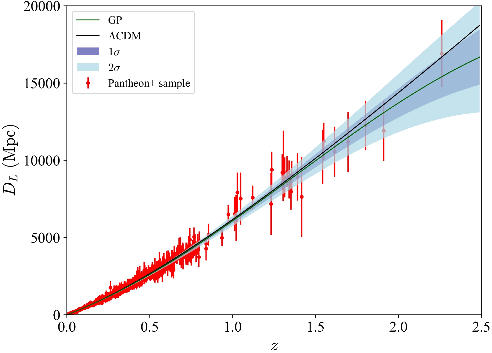
Figure 2. (color online)
$ D_L-z $ relation reconstructed through the Gaussian process from the Pantheon+ at redshift$ z<2.5 $ . The green curve is the central value of the reconstruction whereas the blue regions represent the$ 1\sigma $ and$ 2\sigma $ uncertainties of the reconstruction. The red dots with$ 1\sigma $ error bars are the Pantheon+ data points whereas the black curve represents the best-fitting curve of the ΛCDM model. -
In the standard cosmological model, the relationship between angular-diameter and luminosity distances at redshift z is given by
$ \frac{D_A(z)(1+z)^2}{D_L(z)} = 1, $

(10) which is known as the cosmic DDR. To test the potential violation of the standard DDR, we rewrite it as
$ \frac{D_A(z)(1+z)^2}{D_L(z)} = \eta(z). $

(11) The standard DDR holds when
$ \eta \equiv 1 $ . Deviation of η from unity implies violation of DDR. The parameter η may be redshift-dependent, and various forms of η have been proposed. In this study, we analyzed the violation of DDR using three parameterized models:$ {\rm{Model\ 0}}: \; \eta(z) = 1+\eta_0, $

(12) $ {\rm{Model\ 1}}: \; \eta(z) = 1+\eta_0 z, $

(13) $ {\rm{Model\ 2}}: \; \eta(z) = 1+\eta_0 z/({1+z}), $

(14) where the DDR violation parameter
$ \eta_0 $ is assumed to be constant. The latter two models are designed to explore the possible redshift-dependence of DDR violation.By combining the angular diameter distances from SGL with the corresponding luminosity distances from the GP reconstruction, we can constrain the DDR violation parameter in a cosmological model-independent manner. However, keep in mind that both the
$ D_A $ data points from SGL systems and the$ D_L $ data points from SNe Ia are given in the form of probability distributions. The main processes are summarized as follows:1. For each redshift (four
$ z_l $ and four$ z_s $ ) in the SGL sample, we randomly extracted 1000 values of$ D_A $ from the corresponding probability distribution presented in Section II.A, and randomly extracted 1000 values of$ D_L $ from the corresponding probability distribution presented in Section II.B, resulting in 1000 realizations at each given redshift.2. From these 1000 realizations at each given reshift, we calculated 1000 values of
$ \eta(z) $ according to Eq. (11), thus obtaining the probability distribution of$ \eta(z) $ at each redshift, denoted as$ p_i(\eta(z_i)) $ .3. For a given model, such as Model 1, the joint likelihood can be expressed as
$ {\cal{L}}\propto \prod\limits_{i = 1}^{n}p_i(1+\eta_0z_i) $ , where$ n = 8 $ for the combination of four SGL systems, and$ n = 2 $ for individual SGL systems. For a given redshift z,$p_i(1+\eta_0z_i) = p_i(\eta(z_i))$ , where$ p_i(\eta(z_i)) $ is obtained in Step 2.4. The best-fitting parameter
$ \eta_0 $ for each parameterized model is determined by maximizing the corresponding joint likelihood function.Assuming a flat prior on
$ \eta_0 $ and limiting$ -1\leq\eta_0\leq1 $ , we conducted a Markov-Chain Monte Carlo (MCMC) analysis to calculate the posterior probability density function (PDF) of the parameter space. The best-fitting parameters for the three parameterized models are presented in Table 2 for all SGL systems as well as for each individual SGL system. The corresponding PDFs are presented in Fig. 3. In the framework of Model 0, the parameter is constrained with$ \eta_0 = -0.078_{-0.196}^{+0.200} $ for all SGL systems, indicating that DDR is valid at 1σ confidence level. For the other two redshift-dependent models, there is no strong evidence for the redshift-evolution of DDR. The validity of DDR is verified at 1σ confidence level, with the constraints$ \eta_0 = -0.081_{-0.186}^{+0.195} $ for Model 1 and$\eta_0 = -0.166_{-0.405}^{+0.433}$ for Model 2, respectively.Lens All RXJ1131 $ - $ 1231

PG 1115+080 B1608+656 SDSS 1206+4332 Model 0 $ -0.078_{-0.196}^{+0.200} $ 

$ -0.021_{-0.382}^{+0.386} $ 

$ -0.329_{-0.351}^{+0.380} $ 

$ -0.067_{-0.367}^{+0.371} $ 

$ 0.227_{-0.433}^{+0.425} $ 

Model 1 $ -0.081_{-0.186}^{+0.195} $ 

$ -0.022_{-0.575}^{+0.596} $ 

$ -0.286_{-0.306}^{+0.336} $ 

$ -0.076_{-0.340}^{+0.351} $ 

$ 0.204_{-0.361}^{+0.403} $ 

Model 2 $ -0.166_{-0.405}^{+0.433} $ 

$ -0.029_{-0.631}^{+0.655} $ 

$ -0.386_{-0.425}^{+0.623} $ 

$ -0.090_{-0.553}^{+0.599} $ 

$ 0.210_{-0.628}^{+0.523} $ 

Table 2. Best-fitting parameter
$ \eta_0 $ for the three types of parameterized models.
Figure 3. (color online) Posterior PDFs of
$ \eta_0 $ for three types of parameterized models, constrained from the combination of all four SGL systems, as well as from individual SGL systems.Additionally, we investigated DDR for each SGL system to elucidate their individual contributions to the overall constraint. The results are summarized in Table 2. The corresponding PDFs are plotted in Fig. 3. Within the framework of each parameterized model, the constraint results for each of the four lensing systems consistently indicate the validity of DDR at 1σ confidence level. Notably, for the first three systems, the best-fitting value of
$ \eta_0 $ tends to be negative, which is consistent with the results constrained using all SGL systems. However, for the SDSS 1206+4332 system, the best-fitting value of$ \eta_0 $ tends to be positive, although it is still consistent with zero owing to the large uncertainty. This is because the angular-diameter distances from this SGL system tend to be higher than the prediction of the ΛCDM model (see Fig. 1), while the corresponding luminosity distances are consistent with the ΛCDM prediction within 1σ confidence level. Although the validity of DDR was verified at 1σ confidence level with these four SGL systems, the precision was only at$ 10^{-1} $ level. -
Although hundreds of SGL systems have been observed to date, only a small fraction of them have been subject to time-delay measurement. Leveraging realistic distributions for the properties of lenses and sources, and incorporating magnification bias and detectability of image configurations, Oguri & Marshall [51] conducted a comprehensive analysis of the expected yields for several planned surveys. Their results suggest that the forthcoming wide-field synoptic surveys are likely to identify several thousand lensed quasars in the next few years. In particular, the Large Synoptic Survey Telescope (LSST) is expected to discover over 8000 lensed quasars, and approximately 3000 of them are anticipated to be subject to accurate measurement of time delays. Therefore, we employed Monte Carlo simulations to explore the precision of future datasets in constraining DDR.
To simulate the SGL dataset
$ \{D_A^l, D_A^s\} $ and the corresponding uncertainties, we assumed a fiducial cosmological model to determine the time-delay distance. In the fiducial ΛCDM model, the dimensionless comoving distance from$ z_l $ to$ z_s $ is given by$ \tilde{r}(z_l,z_s) = \int^{z_s}_{z_l}\frac{{\rm d}z}{E(z)}, $

(15) where
$ E(z) = \sqrt{\Omega_m(1+z)^3+1-\Omega_m} $ is the dimensionless Hubble parameter and$ \Omega_m $ represents the normalized matter density. The angular-diameter distance is expressed as$ D_A^{ls} = \frac{1}{1+z_s}\frac{c}{H_0}\tilde{r}(z_l,z_s), $

(16) The time-delay distance
$ D_{\Delta_t} $ can be calculated by combining Eqs. (2) and (16). From Eqs. (2) and (4), the angular-diameter distances of lens and source can be derived as$ D_A^l = \frac{D_{\Delta_t} R_A}{1+z_l}, $

(17) $ D_A^s = \frac{1+z_l}{1+z_s}\frac{D_{\Delta_t} R_A}{1-R_A}, $

(18) where the distance ratio
$ R_A $ is defined by$ R_A\equiv \frac{D_A^{ls}}{D_A^s} = \frac{c^2\theta_E}{4\pi\sigma^2_{\mathrm {SIS}}}, $

(19) where
$ \theta_E $ is the Einstein radius and$ \sigma_{\mathrm{SIS}} $ is the velocity dispersion of the lens galaxy modeled using the singular isothermal sphere (SIS) model. Here, the widely used and well-established SIS model offers a simple and analytically tractable framework to simulate and study the constraints on DDR.The uncertainties of
$ D_A^l $ and$ D_A^s $ are propagated from those of$ R_A $ and$ D_{\Delta_t} $ as follows:$ \frac{\delta D_A^l}{D_A^l} = \frac{1}{1+z_l}\sqrt{\left(\frac{\delta D_{\Delta_t}}{D_{\Delta_t}}\right)^2+\left(\frac{\delta R_A}{R_A}\right)^2}, $

(20) $ \frac{\delta D_A^s}{D_A^s} = \sqrt{\left(\frac{\delta D_{\Delta_t}}{D_{\Delta_t}}\right)^2+\left(\frac{\delta R_A}{R_A(1-R_A)}\right)^2}. $

(21) The uncertainty in
$ D_{\Delta_t} $ propagates from the uncertainties in$ \Delta t $ and$ \Delta\phi $ , while the uncertainty in$ R_A $ propagates from the uncertainties in$ \theta_E $ and$ \sigma_{\mathrm{SIS}} $ , expressed as follows:$ \frac{\delta D_{\Delta t}}{D_{\Delta t}} = \sqrt{\left(\frac{\delta \Delta t}{\Delta t}\right)^2+\left(\frac{\delta \Delta\phi}{\Delta\phi}\right)^2}, $

(22) $ \frac{\delta R_A}{R_A} = \sqrt{\left(\frac{\delta \theta_E}{\theta_E}\right)^2+4\left(\frac{\delta \sigma_{\mathrm{SIS}}}{\sigma_{\mathrm{SIS}}}\right)^2}. $

(23) According to the analysis by Liao et al. [52], the measurement accuracies of
$ \Delta t $ and$ \Delta\phi $ in lensed quasars can reach 3%. The accuracies of$ \theta_E $ and$ \sigma_{\mathrm{SIS}} $ are expected to be approximately 1% and 5%, respectively, in the future LSST survey [53].For the redshift distribution of SGL systems, Oguri & Marshall [51] conducted a detailed analysis of the source redshift distribution of lensed quasars theoretically detectable by the LSST, presenting their findings in Figure 5 of Ref. [51], reproduced here in Fig. 4. For a quasar at redshift
$ z_s $ , the probability density function of the lens redshift at$ z_l $ is given by [54]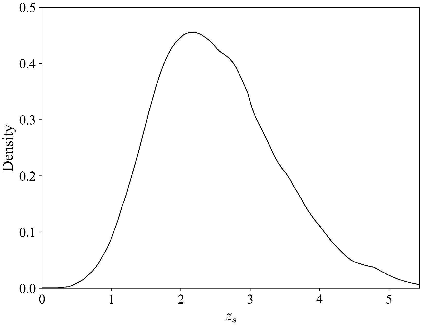
Figure 4. Distribution of
$ z_s $ of lensed quasars as expected in the future LSST survey. Figure reproduced from Ref. [51].$ P(z_l|z_s) = C\frac{\tilde{r}^2(z_l,z_s)\tilde{r}^2(0,z_l)}{\tilde{r}^2(0,z_s)E(z_l)}, $

(24) where C is the normalization constant. Thus, given the redshift of the source, the lens redshift for a SGL system is randomly sampled according to this distribution. It should be mentioned that the redshift of simulated SGL systems is restricted to values below 2.3 owing to the restriction from the maximum redshift of Pantheon+ SNe. Although the combination of high-redshift data such as gamma-ray bursts or gravitational waves can extend beyond the redshift limit of the SNe dataset, the large uncertainties in their calibration would introduce additional complexities and potential systematic errors. The availability and reliability of SNe as standard candles in the redshift range
$ z<2.3 $ can minimize systematic uncertainties associated with the calibration and standardization of$ D_L $ measurements. Therefore, the source redshift in our simulation is restricted to values below 2.3.Assuming that the uncertainties for the parameters
$(\Delta t,\;\Delta\phi,\; \theta_E,\;\sigma_{\mathrm{SIS}})$ are (3%, 3%, 1%, 5%), we can simulate the angular-diameter distances of SGL systems based on the fiducial ΛCDM model, where the cosmological parameters are fixed to be the best-fitting parameter from the Pantheon+ ($ \Omega_m = 0.334 $ ,$ H_0 = 73.6\; {\rm km\; s^{-1}\; {Mpc}^{-1}} $ ) [50]. The procedures are as follows:1. Randomly sample the redshift
$ z_s $ from the source redshift distribution of lensed quasars presented in Fig. 4. If$ z_s>2.3 $ , resample it again; otherwise, continue.2. Given the source redshift
$ z_s $ , sample the lens redshift$ z_l $ according to the distribution given in Eq. (24).3. Calculate
$ D_{\Delta_t} $ and$ R_A $ at$ z_s $ and$ z_l $ by combining Eqs. (2), (15), (16), and (19). The corresponding uncertainties$ \delta D_{\Delta t} $ and$ \delta R_A $ are determined with the assumed parameter accuracies.4. Calculate the fiducial angular-diameter distances
$ \bar{D}_A^l $ and$ \bar{D}_A^s $ according to Eqs. (17) and$ (18) $ , respectively. The corresponding uncertainties$ \delta D_A^l $ and$ \delta D_A^s $ are determined using Eqs. (20) and (21).5. Sample
$ D_A^l $ and$ D_A^s $ from the Gaussian distributions$ D_A^l\sim {\cal{N}}(\bar{D}_A^l,\delta D_A^l) $ and$ D_A^s\sim {\cal{N}}(\bar{D}_A^s,\delta D_A^s) $ . Save the parameter set$(z_s,\;z_l,\;D_A^s, \;\delta D_A^s,\; D_A^l, \; \delta D_A^l)$ as an effective SGL system.We repeated the above steps 100 times to generate 100 SGL systems, resulting in a simulated sample including 200 angular-diameter distances, i.e., 100 values of
$ D_A^l $ and 100 values of$ D_A^s $ . The redshift distributions of$ z_s $ and$ z_l $ in an arbitrary realization of simulation are plotted in the left panel of Fig. 5, and the angular-diameter distances are presented in the right panel of Fig. 5.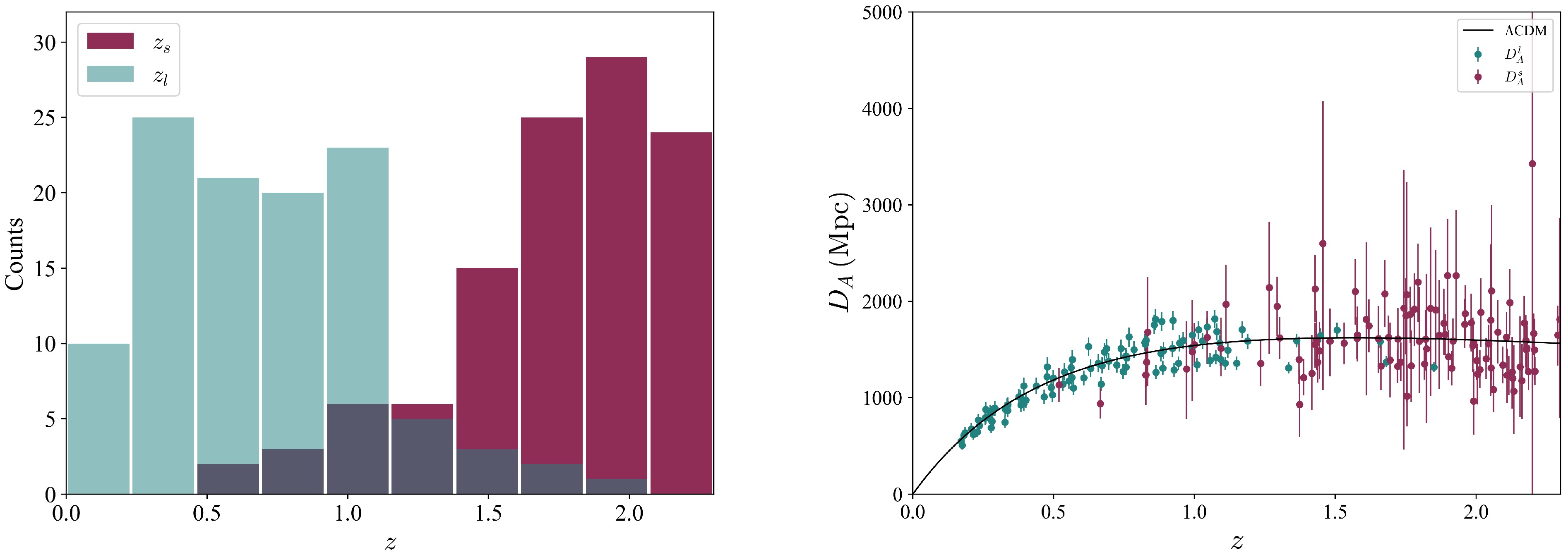
Figure 5. (color online)
$ N = 100 $ mock SGL systems in an arbitrary realization of simulation. Left panel: redshift distribution of$ z_s $ and$ z_l $ ; right panel: angular-diameter distances$ D_A $ and their$ 1\sigma $ uncertainties. The black line is the fiducial ΛCDM curve.Combining the simulated angular-diameter distance sample and the luminosity distance from SNe Ia, we constrained the DDR violation parameter
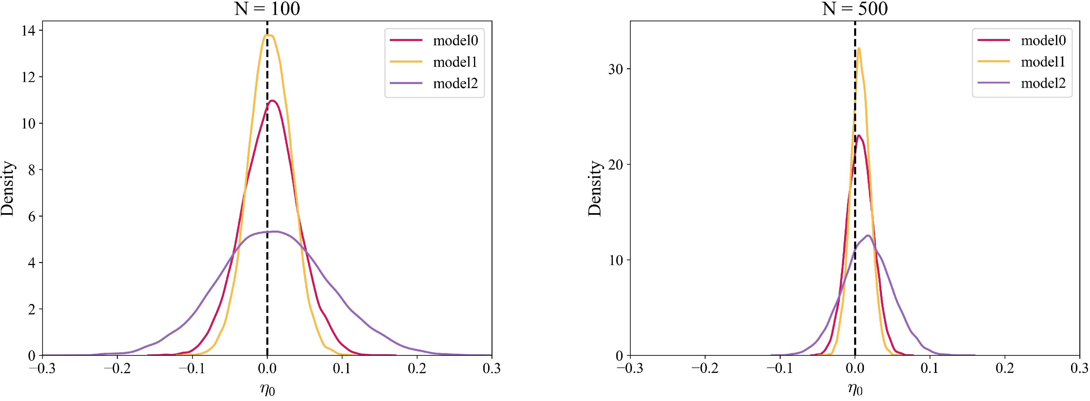
$ \eta_0 $ in three parameterized models as described in Section II.C. The results are presented in Table 3 and Fig. 6. For 100 simulated SGL systems based on future observation accuracy, the parameter$ \eta_0 $ was strictly constrained in the three models, with precision at the$ 10^{-2} $ level. Additionally, we simulated 500 SGL systems to further constrain$ \eta_0 $ , with the results shown in Table 3 and Fig. 6. These simulations indicate that increasing the number of SGL systems from$ N = 100 $ to$ N = 500 $ reduces the uncertainty by an additional factor of two, consistent with the usual$ \sigma\propto N^{-1/2} $ relation.N Model 0 Model 1 Model 2 100 $ 0.004_{-0.038}^{+0.036} $ 

$ 0.004_{-0.028}^{+0.028} $ 

$ 0.008_{-0.071}^{+0.074} $ 

500 $ 0.006_{-0.017}^{+0.017} $ 

$ 0.007_{-0.012}^{+0.013} $ 

$ 0.016_{-0.032}^{+0.033} $ 

Table 3. Best-fitting parameter
$ \eta_0 $ in three parameterized models, constrained from simulated SGL systems. -
Cosmic DDR, which connects angular-diameter and luminosity distances, is a fundamental relation in cosmology. Any deviation from DDR suggests the presence of new physics. Consequently, numerous model-independent methods and datasets have been employed to test DDR. Advancements in observational techniques and data analysis methods are pivotal in reducing uncertainties and enhancing the accuracy of cosmological tests. Recently, the H0LiCOW collaboration constrained the Hubble constant
$ H_0 $ to a precision of 2.4% using six gravitationally lensed quasars with precisely measured time-delay distances. These time-delay distances are related to angular-diameter distances, offering a promising avenue for high-precision DDR tests. In this study, we tested DDR by utilizing the angular-diameter distances from the SGL sample of the H0LiCOW collaboration, which provides precise time-delay and angular-diameter distances to the lens for four SGL systems, along with luminosity distances derived from the latest Pantheon+ compilation of SNe Ia.To minimize the statistical error arising from the redshift matching of SNe Ia with the SGL systems, we employed the GP method to reconstruct the
$ D_L-z $ relation from the Pantheon+ dataset, thereby determining the luminosity distances of the SGL systems. By combining the angular diameter distance from SGL systems with the GP reconstruction of luminosity distence from SNe Ia, we constrained the parameter$ \eta_0 $ , which quantifies potential deviations from the standard DDR, across three parameterized models. The parameter$ \eta_0 $ was constrained to$ \eta_0 = -0.078_{-0.196}^{+0.200} $ in Model 0,$ \eta_0 = -0.081_{-0.186}^{+0.195} $ in Model 1, and$ \eta_0 = -0.166_{-0.405}^{+0.433} $ in Model 2, thus confirming the validity of DDR at the 1σ confidence level. Furthermore, we investigated the potential precision constraints based on the future observational accuracy using Monte Carlo simulations. For 100 simulated SGL systems, the precision of$ \eta_0 $ reached the$ 10^{-2} $ level for the three parameterized models.Previous studies tested DDR by combining different samples. Using the Union2 sample of SNe Ia, Li et al. [16] parameterized DDR with Model 1 and found that DDR is valid at the 1σ confidence level with a constraint of
$ \eta_0 = -0.07^{+0.19}_{-0.19} $ from 18 cluster galaxies; however, it is violated at the 1σ confidence level with a constraint of$ \eta_0 = -0.22^{+0.11}_{-0.11} $ from 38 cluster galaxies. Combining the Einstein angular measurement of 161 SGL systems with JLA sample of SNe Ia, Liao et al. [18] constrained the parameter$ \eta_0 $ of Model 1 to$ \eta_0 = -0.005^{+0.351}_{-0.215} $ . Similarly, combining 205 SGL systems and the Pantheon sample, Zhou et al. [19] constrained$ \eta_0 = 0.047^{+0.190}_{-0.151} $ , verifying the DDR at the 1σ confidence level. In this study, by using only four SGL systems with measured time-delay distance, we achieved a constraint on the DDR parameter with comparable accuracy to that of the aforementioned results. Furthermore, our simulation results suggest that the upcoming observational advancements from the lensed quasars of the LSST survey will significantly enhance the precision of DDR testing.In a previous study conducted by Liao et al. [18], the distance ratio derived from Einstein ring was used to constrain DDR. The Einstein ring depends on the ratio of distance,
$ R_A = D_A^{ls}/D_A^s $ . Although the available sample of SGL systems is large, the ratio of distance may cancel some important information, which may introduce large uncertainty on DDR testing. By contrast, in this study, the degeneracy between$ D_A^{ls} $ and$ D_A^s $ is broken by the observed time delay, and the angular-diameter distances from the observer to the lens and to the source are obtained simultaneously. The direct comparison of angular-diameter and luminosity distances provides a more precise approach to test DDR than using the distance radio. For example, with only four SGL systems, the DDR violation parameter$ \eta_0 $ can be constrained at a precision of$ 0.2 $ in Model 1, which is comparable to the precision of 60 SGL systems obtained in Ref. [18]. However, our method is more susceptible to systematic errors from the absolute calibration of time-delay distances, such as uncertainties in the lens mass distribution, line-of-sight structure, and external convergence effects. In addition, at present, a majority of SGL systems have not been subject to time-delay measurement. Therefore, the available data sample is small. We expect that the LSST survey will provide more time-delayed SGL systems, thereby setting a tight constraint on DDR in the near future.
Cosmic distance duality relation in light of time-delayed strong gravitational lensing
- Received Date: 2024-08-01
- Available Online: 2025-01-15
Abstract: The cosmic distance duality relation (DDR), which links the angular-diameter and luminosity distances, is a cornerstone in modern cosmology. Any deviation from DDR may indicate new physics beyond the standard cosmological model. In this study, we used four high-precision time-delayed strong gravitational lensing (SGL) systems provided by H0LiCOW to test the validity of DDR. To this end, we directly compared the angular-diameter distances from these SGL systems with the luminosity distances from the latest Pantheon+ compilation of SNe Ia. To reduce the statistical errors arising from redshift matching, a Gaussian process method was applied to reconstruct the distance-redshift relation from the Pantheon+ dataset. We parameterized the possible violation of DDR in three different models. All results confirm the validity of DDR at


 Abstract
 HTML
HTML Reference
 Related
 PDF
PDF




 DownLoad: