


 Abstract
 HTML
HTML Reference
 Related
 PDF
PDF


-
As a nonlinear extension of quantum electrodynamics (QED), the Euler-Heisenberg (EH) Lagrangian, formulated in 1936 [1], provides a classical approximation that is superior to Maxwell's equations under strong-field conditions, where vacuum polarization is significant. This framework models the vacuum as a dynamically polarizable medium, with polarization/magnetization arising from virtual charge clouds around real charges/currents [2]. This theory not only provides a more precise classical approximation of QED than Maxwell's electrodynamics under strong-field conditions, it also serves as a foundational tool for studying nonlinear phenomena in both astrophysics and cosmology. In 1956, its unique physical properties were used to find the first EH black hole solution, an anisotropic Reissner-Nordström-like magnetically charged configuration with dyon degrees of freedom [3]. Subsequent studies have focused on electrically charged solutions [3, 4], rotating solutions [5, 6], and frameworks based on modified gravity theories [7, 8]. Very recently, inspired by string theory and Lovelock theory, Ref. [9] proposed an extension of Einstein-Maxwell-dilaton theory by coupling dilaton with EH electrodynamics. Other authors have investigated the effects of particle motion and gravitational lensing on magnetically charged black holes [10, 11] and black hole shadows [12]. Subsequently, Jiang et al. [13] described geometrically thin and optically thick accretion disks around magnetically charged black holes.
Quasinormal modes (QNMs) are fundamental dissipation signatures of spacetime perturbations. They are particularly significant in black hole systems, where energy is lost primarily through radiation to infinity or absorption by the event horizon. The analysis of QNMs provides valuable insights into black hole spacetime geometry and could be instrumental in gravitational wave observations. It can also be useful in exploring fundamental symmetries in gauge/gravity correspondence. Cho et al. [14, 15] introduced the asymptotic iteration method (AIM), a systematic approach for deriving determining accurate approximations of quasinormal frequencies(QNFs). Here, we use the AIM method to solve the perturbation equation numerically. In addition, we utilize the WKB method [16−18], a widely recognized and established technique, to estimate the QNFs of the black holes. We compare the results obtained via the two approaches to validate and strengthen our findings. Another important concept for a black hole perturbation system is the greybody factor [19−22]. It describes the modification of the spectrum of radiation as it escapes the black hole’s gravitational well. In the context of gravitational wave astronomy, the interplay between QNFs and the greybody factor establishes a self-consistent framework for interpreting compact object mergers. QNFs govern the post-merger ringdown phase via their resonant frequencies and damping rates, whereas the greybody factor characterizes the anisotropic emission of gravitational waves during the complete inspiral-merger-ringdown sequence [23].
Based on the above, this study investigates the QNFs and greybody factor of test external fields in magnetically charged black hole spacetimes within the string-inspired Euler–Heisenberg framework. This paper is constructed as follows. In Section II, we review the black hole solution briefly. Then, in Section III, we derive the master equations for test massless scalar and electromagnetic fields. In Section IV, we compute the QNFs using the AIM and WKB methods, and study how they are affected by black hole parameters. In Section V, we calculate the greybody factor using the WKB method. Section VI discusses and concludes the study.
-
Inspired by string theory and Lovelock theory, Bakopoulos et al. [9] recently proposed Einstein-Maxwell-dilaton theory with a dilaton-coupled nonlinear Euler-Heisenberg term
$\begin{aligned}[b] S=\;&\frac{1}{16\pi}\int {\rm d}^4x\sqrt{-g}\Big[R-2\nabla^\mu\phi\nabla_\mu\phi-{\rm e}^{-2\phi}F^2\\&-f(\phi)\left(2\alpha F^\mu_{\; \nu} F^\nu_{\; \rho} F^\rho_{\; \delta} F^\delta_{\; \mu}-\beta F^4\right)\Big],\end{aligned} $

(1) where R denotes the scalar curvature,
$ f(\phi) $ is a coupling function depending on the scalar field ϕ and the Faraday scalar$ F^2=F_{\mu\nu}F^{\mu\nu} $ and$ F^4=F_{\mu\nu}F^{\mu\nu}F_{\rho\delta}F^{\rho\delta} $ , where$ F_{\mu\nu} $ represents the standard field strength$ F_{\mu\nu}=\partial_\mu A_{\nu}-\partial_{\nu}A_{\mu} $ . Here, α and β are coupling constants. For$ \alpha=\beta=0 $ , the model reduces to standard Einstein-Maxwell-dilaton theory.If the
$ f(\phi) $ has the form$ f(\phi)=-[3\text{cosh}(2\phi)+2]\equiv-\frac{1}{2}(3{\rm e}^{-2\phi}+3{\rm e}^{2\phi}+4), $

(2) the action in Eq. (1) becomes a magnetically charged black hole with the metric [9]
$ \mathrm{d}s^2=-h(r)\, \mathrm{\mathrm{d}}t^2+\frac{1}{h(r)}\, \mathrm{d}r^2+R(r)^2\, (\mathrm{d}\theta^2+\sin^2\theta\, \mathrm{d}\varphi^2), $

(3) $ \begin{align} h(r)=&1-\frac{2 M}{r}-\frac{2(\alpha-\beta)Q_m^4}{r^3(r-Q_m^2/M)^3}, \quad R(r)=r\left(r-\frac{Q_m^2}{M}\right),\\ \phi (r)=&-\frac{1}{2}\ln \left(1-\frac{Q_m^2}{M r}\right), \quad A_\mu=(0,\, 0,\, 0,\, Q_m\cos\theta), \end{align} $

(4) where M and
$ Q_m $ are the mass and magnetic charge of the black hole, respectively. For simplicity, we define$ \epsilon= \alpha-\beta $ .It is noteworthy that, in the limit
$ \epsilon=0 $ , Eq. (4) reduces to the Gibbons-Maeda-Garfinkle-Horowitz-Strominger (GMGHS or GHS) black holes [24, 25] and becomes the Schwarzschild solution when$ Q_m=0 $ .To date, these studies have generated substantial interest in the GMGHS (or GHS) black hole solutions [26−29]. In addition, Ref. [9] shows that the solution (4) with$ \epsilon\neq0 $ describes a black hole with a single horizon when$ \epsilon=1 $ and two to none for$ \epsilon=-1 $ , implying the magnetically charged black holes have different horizon structures. Therefore, here, we consider both solutions ($ \epsilon>0 $ and$ \epsilon<0 $ ).From Eqs. (3) and (4), we can also rewrite the old metric (3) to a new spherically symmetric metric ansatz
$ \mathrm{d}s^2=-A(r)\, \mathrm{d}t^2+\frac{1}{B(r)}\, \mathrm{d}r^2+r^2(\mathrm{d}\theta^2+\sin^2\theta\, \mathrm{d}\varphi^2), $

(5) and the magnetically charged black hole solution are obtained as
$ \begin{aligned}[b] A(r)=\;&1-\frac{4 M^2}{Q_m^2+\sqrt{Q_m^4+4 M^2 r^2}}-\frac{2\epsilon Q_m^4}{r^6},\\ B(r)=\;&1 - \frac{Q_{m}^{4} + 4M^{2}r^{2}}{r^2(Q_{m}^{2} + \sqrt{Q_{m}^{4} + 4M^{2}r^{2}})} +\frac{Q_m^4}{4M^2r^2}\\& - \frac{\epsilon Q_{m}^{4}(Q_{m}^{4} + 4M^{2}r^{2})}{2M^2r^{8}},\\ \phi (r)=\;&-\frac{1}{2}\ln \left(\frac{\sqrt{Q_m^4+4 M^2 r^2}-Q_m^2}{\sqrt{Q_m^4+4 M^2 r^2}+Q_m^2}\right) . \end{aligned} $

(6) -
This sections presents the master equations of various external fields, including the scalar field and electromagnetic field around magnetically charged black hole.
-
This scalar perturbation can be treated as a probe in a fixed background geometry, and the corresponding perturbation equation can be written as
$ \Box\Phi=\frac{1}{\sqrt{-g}}\partial_{\mu}\left(\sqrt{-g}g^{\mu\nu}\partial_{\nu}\Phi\right)= 0 . $

(7) Considering Eq. (5), we can use the seperation of variables to Eq. (7) as
$ \Phi(t,r,\theta,\varphi)=\mathrm{e}^{\mathrm{-i}\omega t}\frac{\psi_s(r)}{r}Y(\theta,\varphi). $

(8) Then, the perturbed field equation for the radial part in the tortoise coordinate can be written as
$ \frac{\mathrm{d}^2\psi_s(r_*)}{\mathrm{d}r_*^2}+\left[\omega^2-V_s(r)\right]\psi_s(r_*)=0, $

(9) where the tortoise coordinate
$ r_* $ is defined as follows:$ \mathrm{d}r_*=\frac{1}{\sqrt{A(r)B(r)}}\mathrm{d}r. $

(10) Here,
$ \psi_s(r) $ is a radial wave function, ω is the frequency of Φ, l corresponds to the multipole moment of the black hole’s QNMs, and$ V_s(r) $ is the effective potential$ V_s(r)=\frac{ {A}'(r)B(r)+A(r){B}'(r)}{2r}+\frac{A(r)}{r^2}l(l+1). $

(11) Evidently, this effective potential
$ V_s(r) $ depends on the black hole background as well as multipole moment l. -
The propagation of the massless electromagnetic field in a curved spacetime, minimally coupled to the geometry, is driven by Maxwell’s equations
$ \frac{1}{\sqrt{-g}} \, \partial_\mu \left( \sqrt{-g} \, g^{\sigma\mu}g^{\rho\nu} F_{\rho\sigma}\right)=0, $

(12) where
$ F_{\rho\sigma}=\partial_{\rho}A_{\sigma}-\partial_{\sigma}A_{\rho} $ is the field strength tensor and$ A_{\rho} $ is the vector potential of the perturbed electromagnetic field that can be decomposed as$ \begin{aligned}[b]A_{\rho}(t,r,\theta,\varphi)=\; & \sum\limits_{l,m}^{ }\mathrm{e}^{-\mathrm{i}\omega t}\begin{bmatrix}0 \\ 0 \\ h_0(r)\dfrac{1}{\sin\theta}\dfrac{\partial Y_{l,m}}{\partial\varphi} \\ -h_0(r)\sin\theta\dfrac{\partial Y_{l,m}}{\partial\theta}\end{bmatrix} \\ & +\sum\limits_{l,m}^{ }\mathrm{e}^{-\mathrm{i}\omega t}\begin{bmatrix}h_1(r)Y_{l,m} \\ h_2(r)Y_{l,m} \\ h_3(r)\dfrac{\partial Y_{l,m}}{\partial\theta} \\ h_3(r)\dfrac{\partial Y_{l,m}}{\partial\varphi}\end{bmatrix}.\end{aligned} $

(13) Here,
$ Y_{l,m}(\theta, \varphi) $ are spherical harmonics and l and m are the angular and azimuthal quantum numbers, respectively. The first column in Eq. (13) is the axial component with parity$ (-1)^{l+1} $ and the second term is the polar mode with parity$ (-1)^l $ .Substituting the axial and polar modes of the electromagnetic perturbations into Eq. (12), we obtain
$ \frac{\mathrm{d^2}\Psi_e(r_*)}{\mathrm{d}r_*^2}+\left(\omega^2-V_e(r)\right)\Psi_e(r_*)=0, $

(14) with the potential
$ V_{e}(r) = A(r) \frac{l(l+1)}{r^2} , $

(15) and the function
$ \Psi_e(r) $ takes different forms for the two modes$ \quad \quad \quad \quad \quad \quad \Psi_e(r) = h_0(r), \quad odd \;parity , $

(16) $ \Psi_e(r)=-\sqrt{\frac{B(r)}{A(r)}}\frac{r^2}{l(l+1)}\left(\mathrm{i}\omega h_2(r)+\frac{\mathrm{d}h_1(r)}{\mathrm{d}r}\right),\quad even\; parity. $

(17) Note that the solutions in Eq. (6) are invariant under the following rescaling:
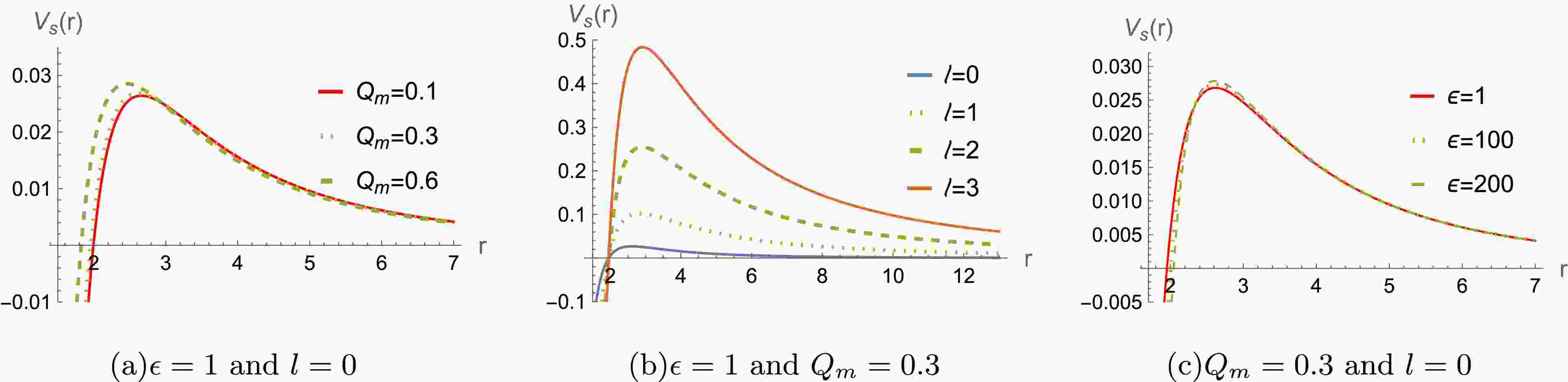
$ r/M\rightarrow r $ ,$ Q_m /M\rightarrow Q_m $ , and$ \epsilon/ M^2\rightarrow \epsilon $ . For a better analysis of the potential function's behavior, we set$ M=1 $ throughout the paper and leave$ \epsilon $ and$ Q_m $ free without loss of generality. The effective potentials$ V_s(r) $ and$ V_e(r) $ are plotted in Figs. 1−4. Figs. 1 and 2 shows that the height of the potentials$ V_s(r) $ increases with the$ Q_m $ and multipole moment l ( for both$ \epsilon<0 $ and$ \epsilon>0 $ ). However, the difference between the effective potentials obtained using the two$ \epsilon $ is very small. The similar phenomena also appear for the effective potentials$ V_e(r) $ of the massless electromagnetic field. In addition, the effective potentials are always positive in Figs. 1−4, indicating that the system is stable under the perturbations of the scalar and electromagnetic fields.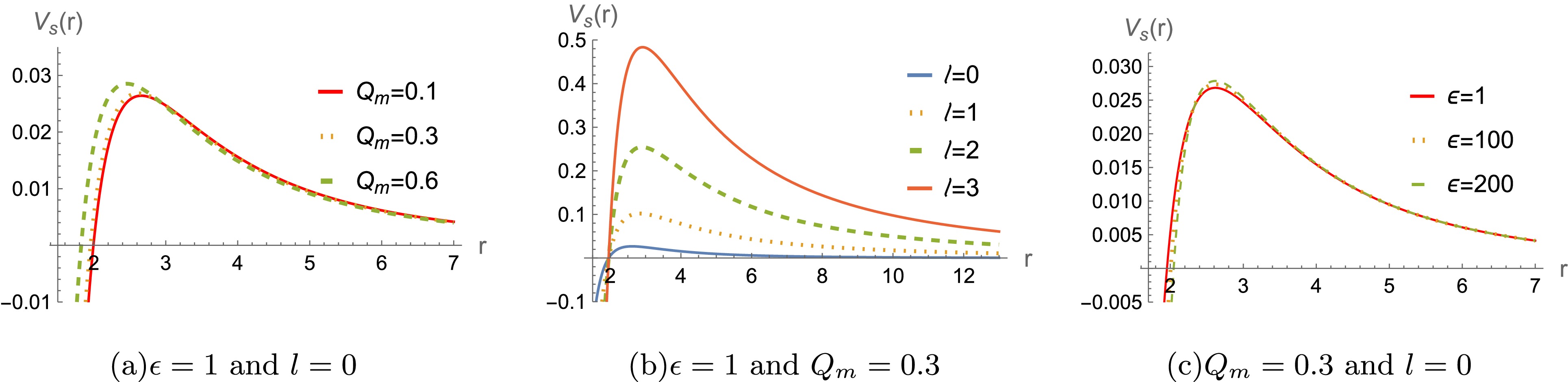
Figure 1. (color online) The effective potential
$ V_s(r) $ for massless scalar field perturbation for a black hole with$ M=1 $ and$ \epsilon>0 $ 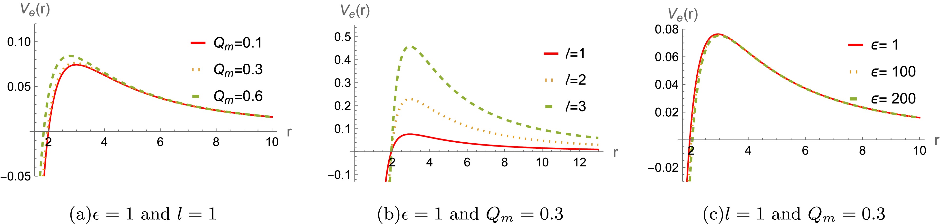
Figure 3. (color online) The effective potential
$ V_e(r) $ for a massless electromagnetic field for a black hole with$ M=1 $ and$ \epsilon>0 $ 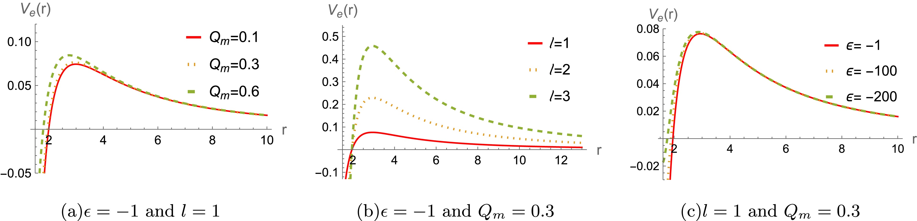
Figure 4. (color online) The effective potential
$ V_e(r) $ for massless a electromagnetic field for a black hole with$ M=1 $ and$ \epsilon<0 $ 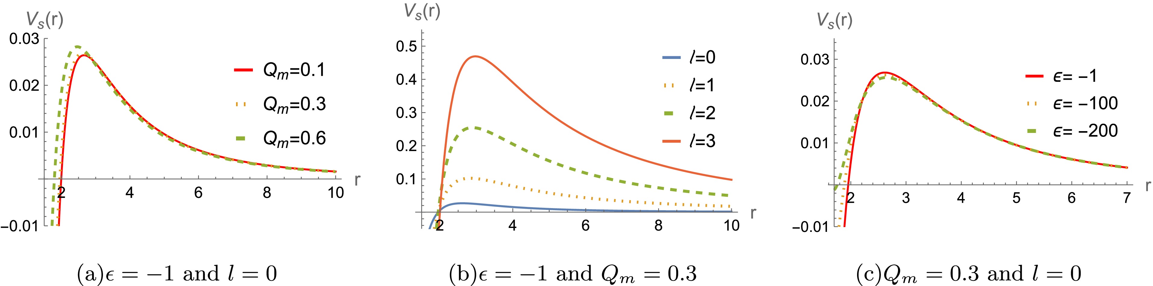
Figure 2. (color online) The effective potential
$ V_s(r) $ for massless scalar field perturbation for a black hole with$ M=1 $ and$ \epsilon<0 $ -
Based on the effective potentials obtained above, we can study the QNFs of magnetically charged black holes in string-inspired Euler-Heisenberg theory. QNFs ω are proper oscillation frequencies corresponding to the solutions of perturbed field equations when appropriate boundary conditions are applied:
$ \psi(r_*)\sim\mathrm{e}^{-\mathrm{i}\omega r_*},\quad r_*=-\infty, $

(18) $ \psi(r_*)\sim\mathrm{e}^{\mathrm{i}\omega r_*},\quad r_*=+\infty, $

(19) where purely ingoing modes occur at
$ r_{*} \to -\infty $ (at the event horizon) and purely outgoing modes occur at$ r_{*} \to +\infty $ (at the spatial infinity).In general, the perturbed field equations (Eqs. (9) and (14)) cannot be derived analytically. In this section, we introduce two different methods, AIM and the 6th-order WKB approximation method to calculate the QNFs of magnetically charged black holes and compare the results. To streamline the discussion, we provide a concise overview of the WKB and AIM methods in Appendices A and B. We also calculate the percentage deviation
$ \Delta_{AW} $ of QNFs obtained via the AIM and WKB methods. The relative error$ \Delta_{AW} $ between the two methods is defined by$ \Delta_{AW}=\frac{|\omega_{AIM}-\omega_{WKB}|}{|\omega_{WKB}|}\times 100{\text{%}}. $

(20) By taking different values of
$ Q_m $ for the two solution branches, these fundamental QNFs$ (n=0) $ are obtained for various massless fied perturbations, as shown in Tables 1 and 2. The fundamental QNFs obtained by numerical methods agree well with each other for each solution branch. From Table 1, the relative error$ \Delta_{AW} $ decreases significantly as l increases. These results are consistent with the characteristic features of the WKB method.$ \epsilon=1 $ 

$ \epsilon=-1 $ 

l $ Q_m $ 

AIM WKB $ \Delta_{AW} $ (%)

AIM WKB $ \Delta_{AW} $ (%)

0 0.1 $ 0.110562-0.105038${\rm i}$ $ 

$ 0.110661 - 0.100865 ${\rm i}$ $ 

2.78754 $ 0.110562 -0.105037${\rm i}$ $ 

$ 0.110663 - 0.100869 ${\rm i}$ $ 

2.78412 0.3 $ 0.112132-0.105410${\rm i}$ $ 

$ 0.112306 - 0.100973 ${\rm i}$ $ 

2.94067 $ 0.112159-0.105337${\rm i}$ $ 

$ 0.112202 - 0.101578 ${\rm i}$ $ 

2.48424 0.5 $ 0.115402-0.106452${\rm i}$ $ 

$ 0.116533 - 0.0984805 ${\rm i}$ $ 

5.27728 $ 0.115647-0.105672${\rm i}$ $ 

$ 0.115833 - 0.103841 ${\rm i}$ $ 

1.18288 0.6 $ 0.117741-0.107542${\rm i}$ $ 

$ 0.116024 - 0.117945 ${\rm i}$ $ 

6.37286 $ 0.118292-0.105480${\rm i}$ $ 

$ 0.11782 - 0.105505 ${\rm i}$ $ 

0.29896 1 0.1 $ 0.293432 -0.097712${\rm i}$ $ 

$ 0.293406 - 0.097812 ${\rm i}$ $ 

0.0335086 $ 0.293432 -0.0977110${\rm i}$ $ 

$ 0.293406 - 0.0978113 ${\rm i}$ $ 

0.0334659 0.3 $ 0.297489-0.098155${\rm i}$ $ 

$ 0.29746 - 0.0982498 ${\rm i}$ $ 

0.0316443 $ 0.297510 -0.098099${\rm i}$ $ 

$ 0.297498 - 0.0981848 ${\rm i}$ $ 

0.0276553 0.5 $ 0.306120 -0.099281${\rm i}$ $ 

$ 0.306016 - 0.0994115 ${\rm i}$ $ 

0.0519862 $ 0.306319-0.0986953${\rm i}$ $ 

$ 0.306398 - 0.0986996${\rm i}$ $ 

0.0377309 0.6 $ 0.312483 -0.100351${\rm i}$ $ 

$ 0.312211 - 0.100587 ${\rm i}$ $ 

0.109943 $ 0.312951-0.0986953${\rm i}$ $ 

$ 0.313167 - 0.0988303 ${\rm i}$ $ 

0.0783964 Table 1. The fundamental QNFs
$ (n=0) $ for scalar perturbation with$ M=1 $ .$ \epsilon=1 $ 

$ \epsilon=-1 $ 

l $ Q_m $ 

AIM WKB $ \Delta_{AW} $ (%)

AIM WKB $ \Delta_{AW} $ (%)

1 0.1 $ 0.248737 -0.0925503${\rm i}$ $ 

$ 0.248665 - 0.0927009 ${\rm i}$ $ 

0.0628748 $ 0.248737 -0.0925489${\rm i}$ $ 

$ 0.248666 - 0.0927 ${\rm i}$ $ 

0.0630446 0.3 $ 0.252604 -0.0930818${\rm i}$ $ 

$ 0.252514 - 0.0932532 ${\rm i}$ $ 

0.121663 $ 0.252646 -0.0930246${\rm i}$ $ 

$ 0.252592 - 0.0931737 ${\rm i}$ $ 

0.0588877 0.5 $ 0.260752 -0.0944050${\rm i}$ $ 

$ 0.260503 - 0.0946895${\rm i}$ $ 

0.227963 $ 0.261178 -0.0937916${\rm i}$ $ 

$ 0.261284 - 0.0938366 ${\rm i}$ $ 

0.0417106 0.6 $ 0.306120 -0.0992805${\rm i}$ $ 

$ 0.306016 - 0.0994115 ${\rm i}$ $ 

0.0519862 $ 0.306319-0.0986953${\rm i}$ $ 

$ 0.306398 - 0.0986996${\rm i}$ $ 

0.0377309 2 0.1 $ 0.458394-0.0950606${\rm i}$ $ 

$ 0.458392 - 0.0950673 ${\rm i}$ $ 

0.00151693 $ 0.458394 -0.0950600${\rm i}$ $ 

$ 0.458392 - 0.0950673 ${\rm i}$ $ 

0.00165983 0.3 $ 0.464925-0.0955397${\rm i}$ $ 

$ 0.464922 - 0.0955477 ${\rm i}$ $ 

0.00178846 $ 0.464967 -0.0954883${\rm i}$ $ 

$ 0.464922 - 0.0955477 ${\rm i}$ $ 

0.0156059 0.5 $ 0.478801, -0.0967266${\rm i}$ $ 

$ 0.47879 - 0.0967427 ${\rm i}$ $ 

0.00394474 $ 0.479212 -0.0961876${\rm i}$ $ 

$ 0.479218 - 0.0961862 ${\rm i}$ $ 

0.00130171 0.6 $ 0.488995-0.0978241${\rm i}$ $ 

$ 0.488972 - 0.0978537 ${\rm i}$ $ 

0.00759593 $ 0.490021 -0.0964230${\rm i}$ $ 

$ 0.490039 - 0.0964063 ${\rm i}$ $ 

0.00494179 Table 2. The fundamental QNFs
$ (n=0) $ for electromagnetic perturbation with$ M=1 $ .As l is further increased, the gap among the fundamental QNFs for massless perturbing fields gradually decreases, as shown in Fig. 5. This is because for large l, the dominant terms in all the effective potentials (Eqs. (11) and (15)) are
$ l^2 $ terms and have the same formula in all cases.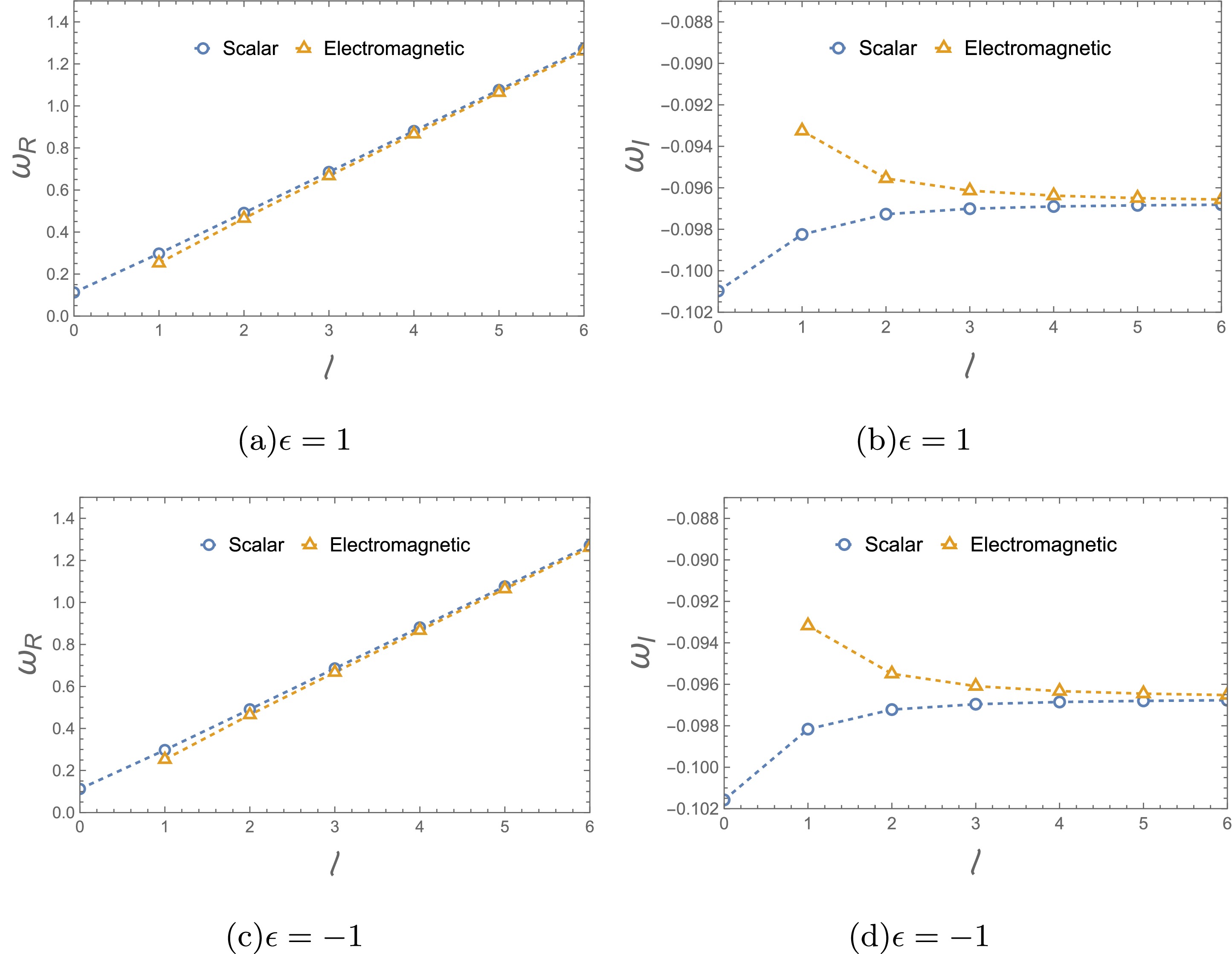
Figure 5. (color online) Variation of fundamental QNFs for different l with
$ M=1 $ and$ Q_m=0.3 $ . -
Now we analyze the influence of the magnetic charge
$ Q_m $ on the QNFs in various external field perturbations. The fundamental QNFs for different values of$ Q_m $ are plotted in Figs. 6 and 7. For black holes from different branches, the QNFs exhibit distinct characteristics under each type of test field perturbation with increasing$ Q_m $ . However, for black holes within the same branch, they have the same trend for scalar and electromagnetic perturbations with varitions in$ Q_m $ .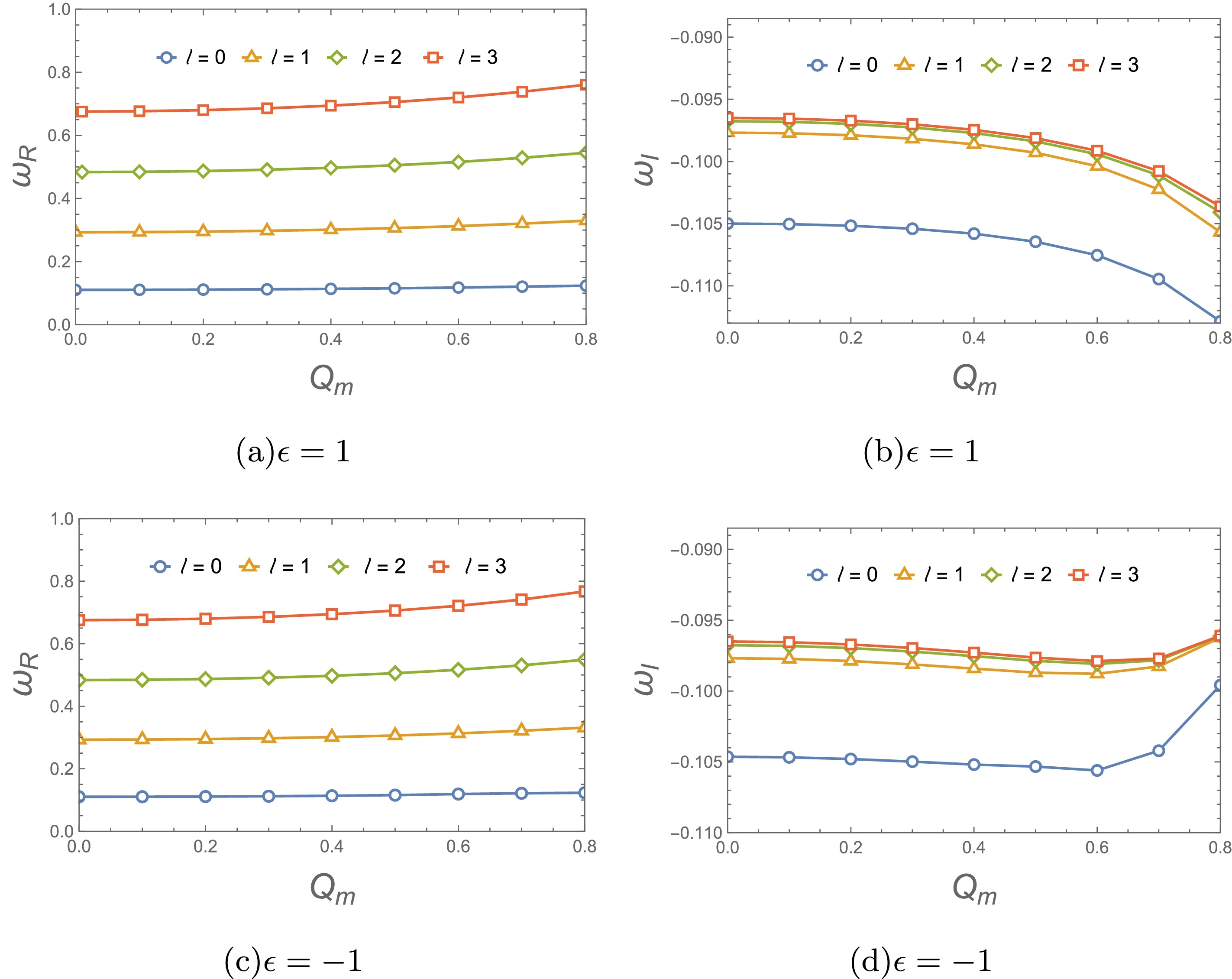
Figure 6. (color online) Variation of scalar fundamental QNFs with respect to the magnetic charge
$ Q_m $ with$ M=1 $ .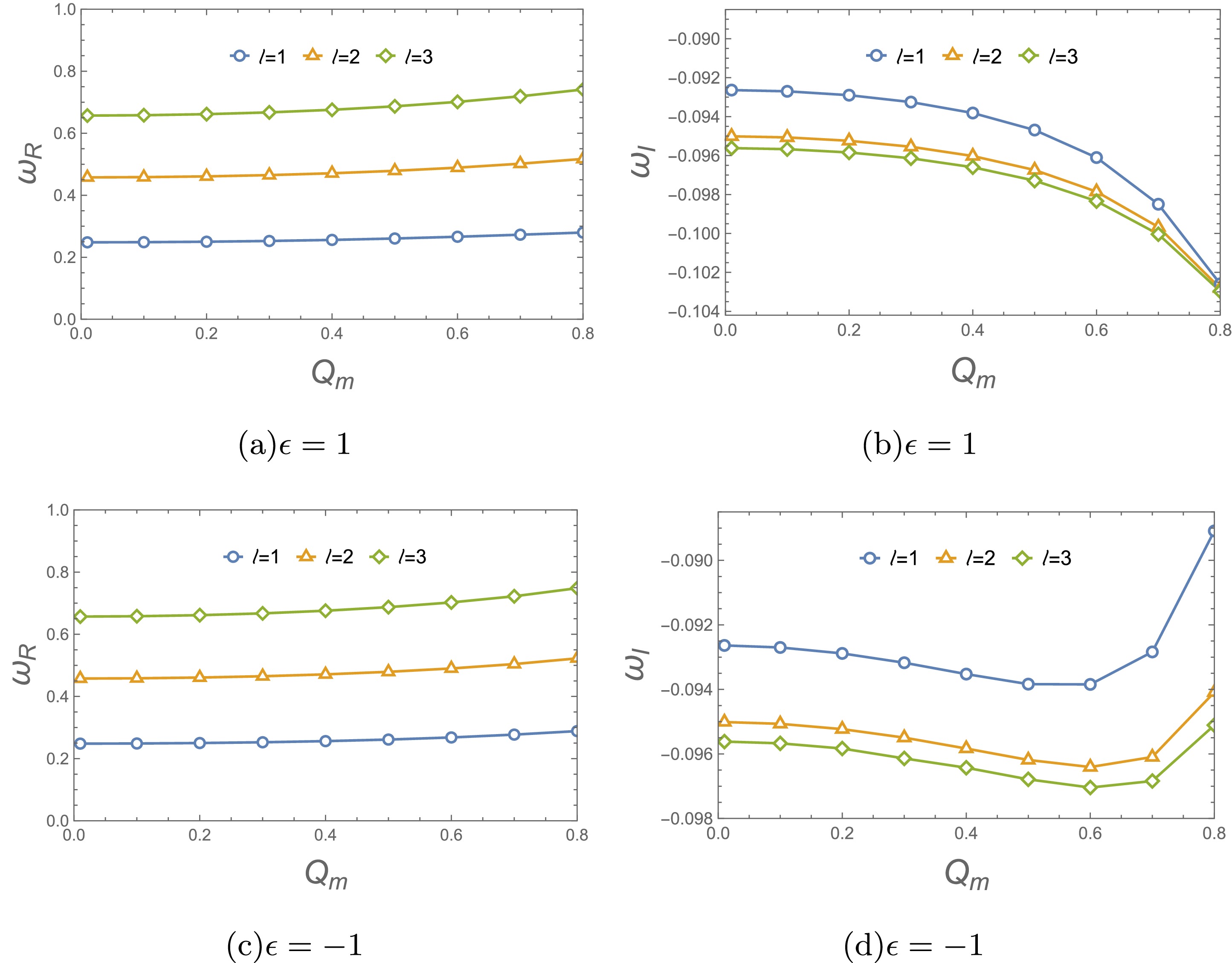
Figure 7. (color online) Variation of electromagnetic fundamental QNFs for different
$ Q_m $ with$ M=1 $ .Taking scalar field perturbation for example, the real QNFs for
$ \epsilon=1 $ increase with$ Q_m $ , and the damping rate or decay rate of the perturbed field increases significantly with increasing$ Q_m $ , as shown in Figs. 6(a) and 6(b). For$ \epsilon=-1 $ (shown in Figs. 6(c) and 6(d)), the real QNFs increase with$ Q_m $ . However, the damping rate increases with$ Q_m $ , and a maximum decay rate is reached at$ Q_m=0.6 $ . As$ Q_m $ surpasses this point, the damping rate begins to decrease. Similar behaviors is also observed for the electromagnetic field perturbation, as shown in Fig. 7.In addition, we check how the magnetic charge
$ Q_m $ influences the evolution and waveform of various perturbations. For more details, see Appendix C. The results for the lowest-lying modes are shown in Fig. 8. For the test scalar field perturbation on the black hole with$ \epsilon=1 $ (see Fig. 8(a)), we observe that large$ Q_m $ makes the ringing stage of perturbation waveforms more intensive but shorter, which corresponds to a larger$ Re(\omega) $ and absolute value of$ Im(\omega) $ (see Figs. 6(a)). In Figs. 8(b) and 8(d), perturbation waves with$ Q_m=0.6 $ have a shorter ringing stage, indicating that they have a larger absolute value of$ Im(\omega) $ . This observation in the time domain is in good agreement with the results obtained in the frequency domain for the black hole with$ \epsilon=-1 $ , as shown in Figs. 6(d) and 7(c).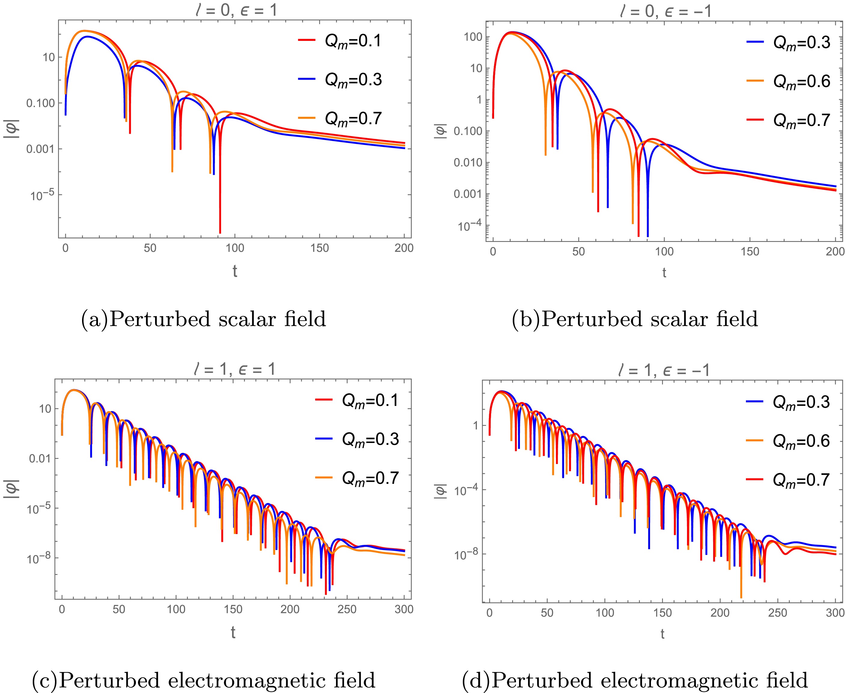
Figure 8. (color online) Time evolution for the perturbed scalar and electromagnetic fields with
$ M=1 $ . -
It is also interesting to investigate the effect of parameter
$ \epsilon $ on the QNFs for scalar and electromagnetic perturbations. When the magnetic charge is fixed at$ Q_m= 0.1 $ , the variation of the fundamental QNFs and damping rate for different values of$ \epsilon $ in is shown in Figs. 9 and 10. For different$ \epsilon $ , the real and imaginary parts of these QNFs remain almost unchanged. These behaviors correspond to the potential function graphs (see Figs. 1(c) and 2(c)), including the propagation of these test fields in time domain (see Fig. 11).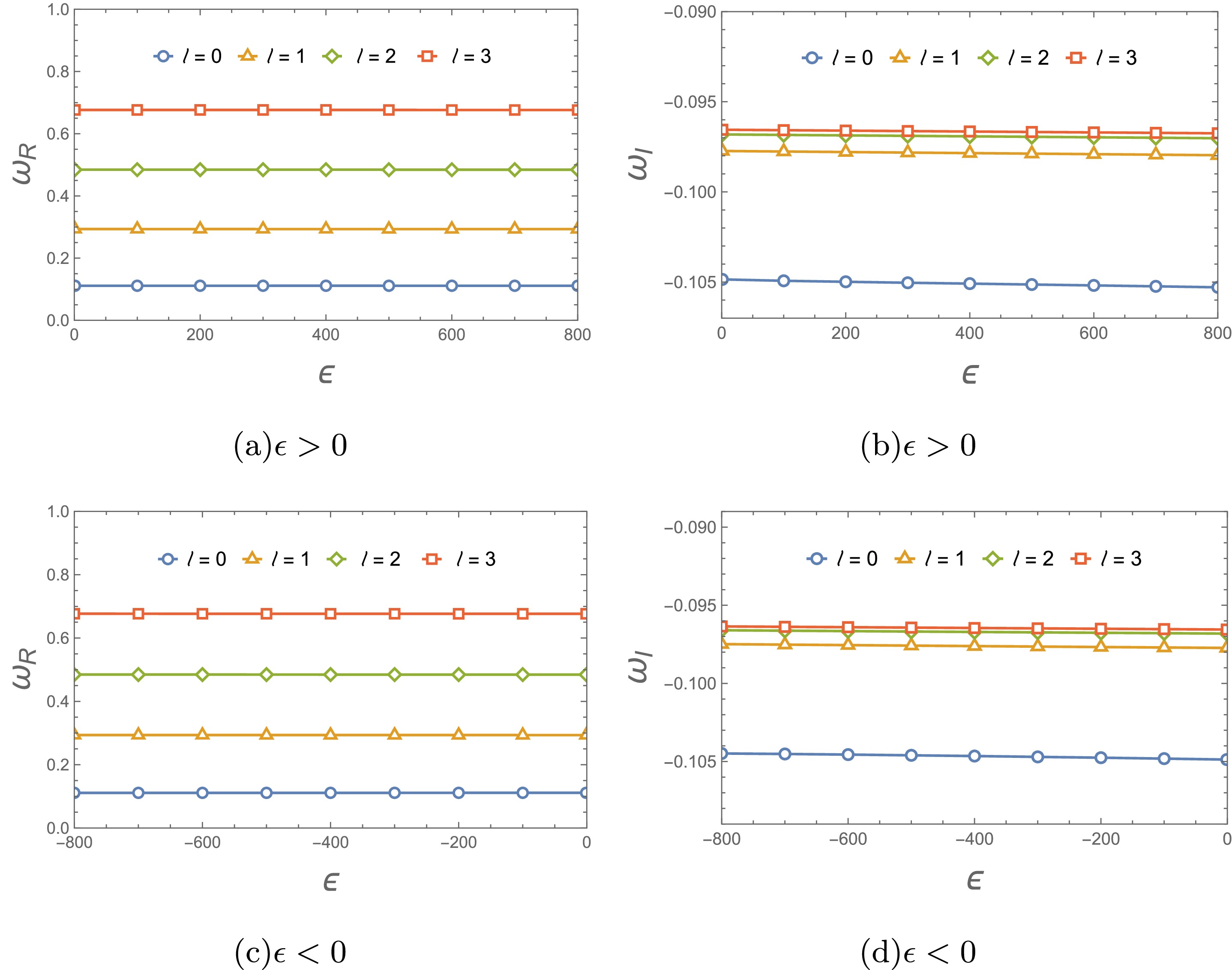
Figure 9. (color online) Variation of scalar fundamental QNFs for different
$ \epsilon $ with$ Q_m=0.1 $ and$ M=1 $ .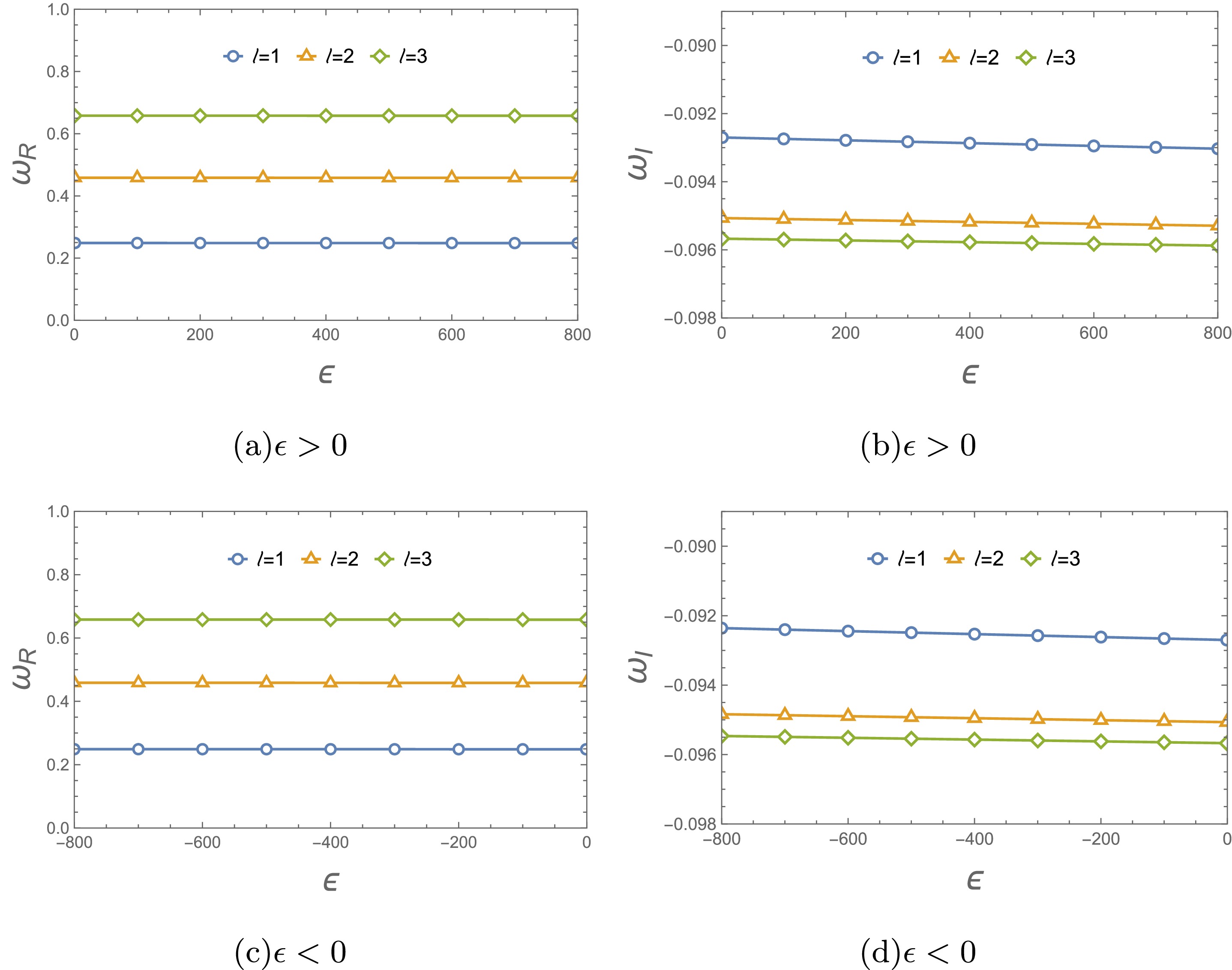
Figure 10. (color online) Variation of electromagnetic fundamental QNFs for different
$ \epsilon $ with$ M=1 $ .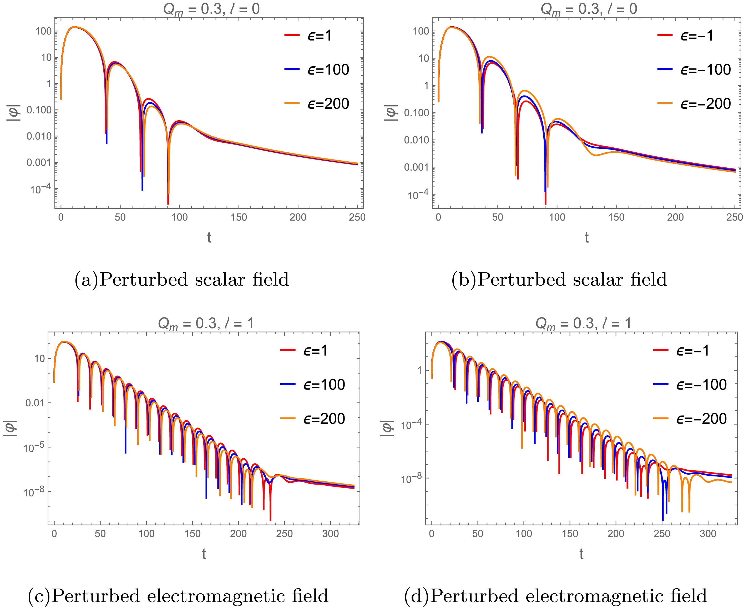
Figure 11. (color online) Time evolution for perturbed scalar and electromagnetic fields with
$ M=1 $ . -
In this section, we use the WKB approximation method to calculate greybody factors for scalar perturbation. The boundary condition for the scattering process is different from that of the QNMs, which can be written as
$ \begin{aligned}[b]\psi= & T(\omega)\mathrm{e}^{-\mathrm{i}\omega r_*},\quad r_*\rightarrow-\infty, \\ \psi= & \mathrm{e}^{-\mathrm{i}\omega r_*}+R(\omega)\mathrm{e}^{\mathrm{i}\omega r_*},\quad r_*\rightarrow+\infty,\end{aligned} $

(21) where R and T represent the reflection coefficient and transmission coefficient, respectively. The greybody factor is defined as the probability of an outgoing wave reaching to infinity or an incoming wave absorbed by the black hole. Therefore,
$ |T(\omega)|^2 $ is called the greybody factor, and$ R(\omega) $ and$ T(\omega) $ should satisfy the following relation$ |R(\omega)|^2+|T(\omega)|^2=1. $

(22) Using the 6th-order WKB method, the reflection and transmission coefficients can be obtained
$ \begin{aligned}[b]|R(\omega)|^2=\; & \frac{1}{1+\mathrm{e}^{-2\pi\mathrm{i}K(\omega)}}, \\ |T(\omega)|^2=\; & \frac{1}{1+\mathrm{e}^{2\pi\mathrm{i}K(\omega)}}=1-|R(\omega)|^2,\end{aligned} $

(23) where K is a parameter that can be obtained by the WKB formula
$ K= \frac{{\rm i}\left( \omega^2 - V(r_0) \right)}{\sqrt{-2V''(r_0)}} + \sum\limits_{i=2}^6 \Lambda_i. $

(24) Figures 12 and 13 show a detailed analysis of the behavior of the greybody factors for massless scalar and electromagnetic perturbations for different magnetic charge
$ Q_m $ and parameter$ \epsilon $ . The greybody factors decrease with$ Q_m $ , indicating that a smaller fraction of the perturbed field can penetrate the potential barrier. We further present the influence of changing$ \epsilon $ on the greybody factors in Figs. 12(c), 12(d), 13(c) and 13(d). As$ \epsilon $ increases, the greybody factors also gradually increase. This indicates that black holes become less interactive with surrounding radiation, allowing more of the perturbed field to escape. These observations are consistent with the behavior of the effective potentials in Figs. 1−4.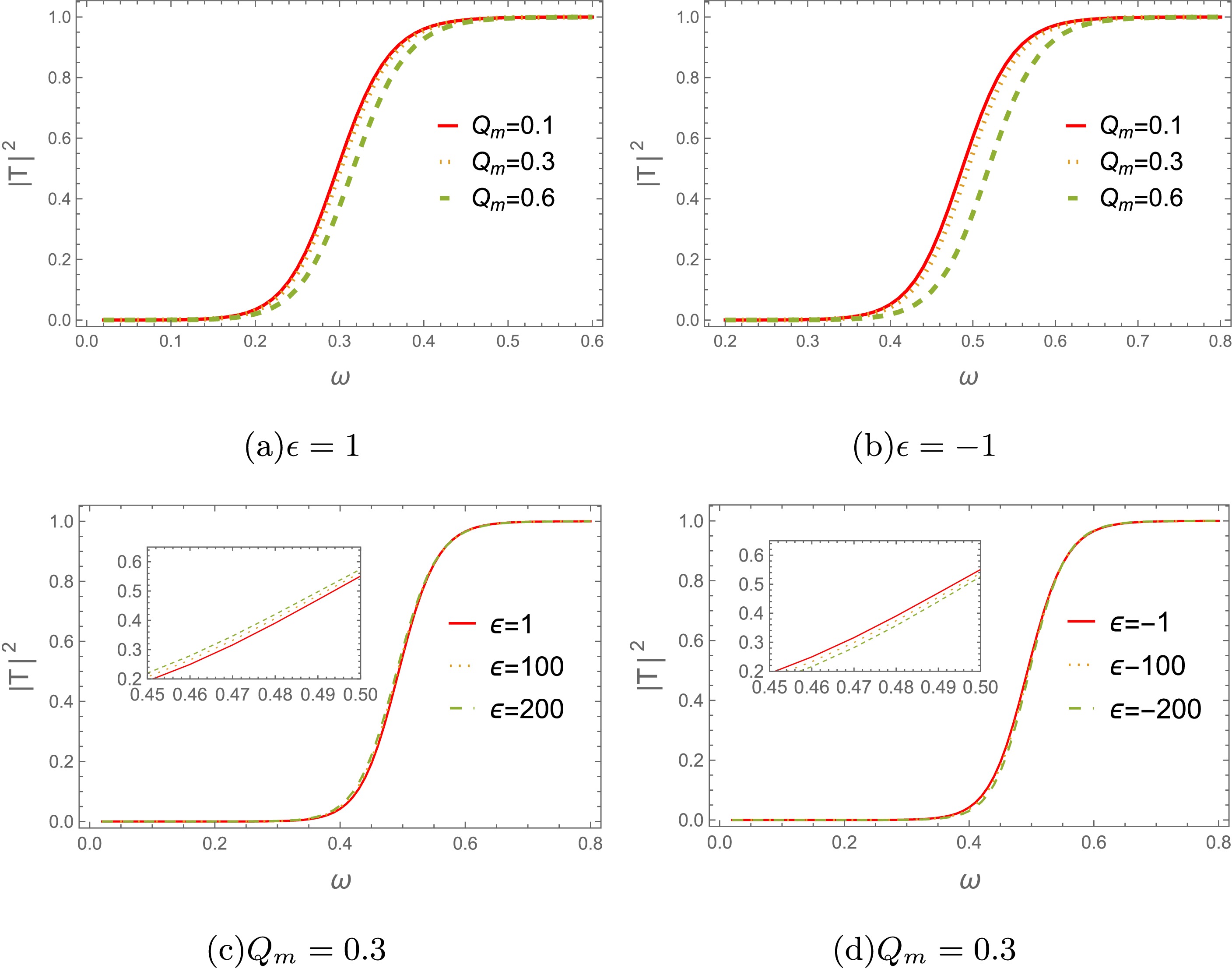
Figure 12. (color online) The scalar field greybody factor vs.
$ Q_m $ with$ M=1 $ .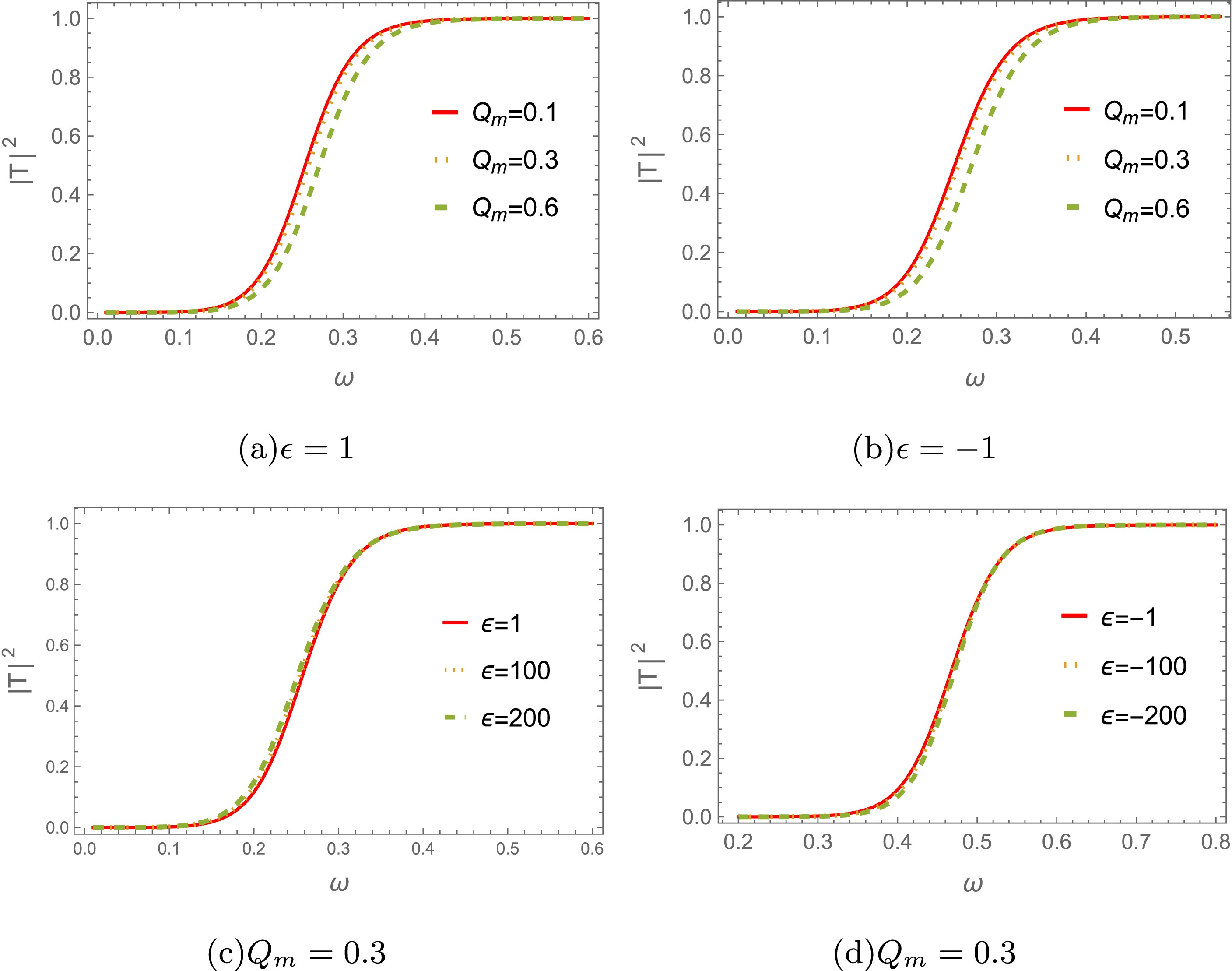
Figure 13. (color online) The electromagnetic field greybody factor vs.
$ \epsilon $ with$ M=1 $ . -
In this paper, we investigated the perturbations of various test fields on magnetically charged black holes within the string-inspired Euler–Heisenberg framework, which features a scalar field ϕ coupled to the electromagnetic field through a coupling function
$ f(\phi) $ . We found that this black hole solution reduces the form of GMGHS or GHS black holes, as$ \epsilon $ tends toward 0. Moreover, this black hole possesses different horizon structures for$ \epsilon>0 $ and$ \epsilon<0 $ . The influence of the magnetic charge$ Q_m $ , parameter$ \epsilon $ , and angular quantum number l on the corresponding effective potentials of the perturbations were analysed.We then employed both the AIM and the WKB approximation to compute the quasinormal frequencies (QNFs) in each scenario. To enhance numerical accuracy, the WKB method was extended to the sixth order. We analyzed how QNFs change with the magnetic charge
$ Q_m $ and different$ \epsilon $ . For$ \epsilon=1 $ , we found that the real QNFs increase as$ Q_m $ increases, and the damping rate or decay rate of gravitational waves increases significantly with increasing$ Q_m $ . For$ \epsilon=-1 $ , the real QNFs increase with$ Q_m $ . However, the damping rate increases with$ Q_m $ and reaches a maximum decay rate occurring at$ Q_m=0.6 $ . As$ Q_m $ surpasses this point, the damping rate begins to slowly. In contrast, we found that the real part and damping rate of the fundamental QNFs remain almost constant for varying$ \epsilon $ . These frequency domain observations agree well with results obtained in the time domain for the two branches of black hole solutions.Using the 6th order WKB method, we also calculated the greybody factor for the perturbed scalar field. The results are shown in Figs. 12 and 13. The effect of the magnetic charge
$ Q_m $ shows that a smaller fraction of the perturbed field can penetrate the potential barrier. Conversely, an opposing phenomenon emerges under the variation of$ \epsilon $ . These results consistent with the effective potentials. -
Tis appendix discusses the main steps of the AIM method. First, we rewrite scalar perturbed Eq. (9) in terms of
$ u=1-r_+/r $ $ \psi''(u)+\frac{1}{2} \left(\frac{A'(u)}{A(u)}+\frac{B'(u)}{B(u)}+\frac{4}{u-1}\right) \psi'(u) +\left[\frac{r_+^2 \omega ^2}{(u-1)^4 A(u) B(u)}+\frac{A'(u)}{2 (u-1) A(u)}+\frac{B'(u)}{2 (u-1) B(u)}-\frac{l (l+1)}{(u-1)^2 B(u)} \right]\psi(u)=0. $

(A1) Evidently, the range of u satisfies
$ 0\leqslant u<1 $ .From Eq. (A1), we consider the behavior of the function
$ \psi(u) $ at the horizon$ (u=0) $ and at the boundary$ u=1 $ . Near the horizon$ (u=0) $ , we have$ A(0)\approx u A'(0) $ and$ B(0)\approx u B'(0) $ . Then, Eq. (A1) becomes$ \psi''(u)+\frac{1}{u}\psi'(u)+\frac{r_+^2\omega^2}{u^2 A'(0) B'(0)}\psi(u)=0. $

(A2) We can obtain the solution
$ \psi(u\to 0)\sim C_1 u^{-\xi}+C_2 u^{\xi}, $

(A3) with
$ \xi=\dfrac{\mathrm{i}r_+\omega}{\sqrt{A'(0)B'(0)}} $ . Then, we set$ C_2=0 $ to impose the ingoing wave condition at the black hole horizon.At infinity
$ (u=1) $ , the asymptotic form of Eq. (A1) can be written as$ \psi''(u)-\frac{2}{1-u}\psi'(u)+\frac{r_+^2\omega^2}{(1-u)^4}\psi(u)=0, $

(A4) with
$ A(1)=1 $ and$ B(1)=1 $ . Then, we can obtain the solution$\begin{aligned}[b]& \psi(u\to 1)\sim D_1 {\rm e}^{-\zeta}+D_2 {\rm e}^{\zeta},\;\\& \zeta=\frac{{\rm i}r_+\omega}{1-u}.\end{aligned} $

(A5) To impose the outgoing boundary condition, we set
$ D_1=0 $ .Now, using the above solutions at horizon and infinity, we can define the general ansatz for Eq. (A1) as
$ \psi(u)=u^{-\xi}{\rm e}^{\zeta}\chi(u) . $

(A6) Substituting Eq. (A6) to Eq. (A1), we have
$ \chi''=\lambda_0(u)\chi'+s_0(u)\chi , $

(A7) where
$ \lambda_0(u)=\frac{1}{2} \left(\frac{4 {\rm i} r_+ \omega }{u \sqrt{A'(0)} \sqrt{B'(0)}}-\frac{A'(u)}{A(u)}-\frac{B'(u)}{B(u)}-\frac{4 \left({\rm i} r_+ \omega +u-1\right)}{(u-1)^2}\right), $

(A8) and
$ \begin{aligned}[b] s_0(u)=\;&\frac{1}{2 (u-1)^4 u^2 A(u) A'(0) B(u) B'(0)}\Big[ {\rm i} r_+ (u-1)^4 u \omega \sqrt{A'(0)} B(u) \sqrt{B'(0)} A'(u) \\ &-u^2 A'(0) B'(0) \left(2 r_+^2 \omega ^2+(u-1)^2 B(u) A'(u) \left({\rm i} r_+ \omega +u-1\right)\right) \\ &+A(u) \Bigg(2 l (l+1) u^2 (u-1)^2 A'(0) B'(0) -u^2 (u-1)^2 A'(0) B'(0) B'(u) \left({\rm i} r_+ \omega +u-1\right)+{\rm i} r_+ u (u-1)^4 \omega \sqrt{A'(0)} \sqrt{B'(0)} B'(u)\\ &+2 r_+ \omega B(u) \Big({\rm r}_+ \omega \left((u-1)^2-u \sqrt{A'(0)} \sqrt{B'(0)}\right)^2+{\rm i} (u+1) (u-1)^3 \sqrt{A'(0)} \sqrt{B'(0)}\Big)\Bigg) \Big]. \end{aligned} $

(A9) Based on
$ \lambda_0 $ and$ s_0 $ , the perturbed equation (A7) can be solved numerically by using the improved AIM [14].Following the same procedure described above, we can also obtain functions
$ \lambda_0 $ and$ s_0 $ for the electromagnetic field perturbation:$ \lambda_0(u)=\frac{1}{2} \left(\frac{4 {\rm i} r_+ \omega }{u \sqrt{A'(0)} \sqrt{B'(0)}}-\frac{A'(u)}{A(u)}-\frac{B'(u)}{B(u)}-\frac{4 \left(i r_+ \omega +u-1\right)}{(u-1)^2}\right), $

(A10) and
$ \begin{aligned}[b] s_0(u)=\;&\frac{1}{2 (u-1)^4 u^2 A(u) A'(0) B(u) B'(0)}\Big[r_+ (u-1)^4 u \omega B(u) \sqrt{A'(0)} A'(u) \sqrt{B'(0)} - r_+ u^2 \omega A'(0) \left(2 r_+ \omega + {\rm i} ( u-1)^2 B(u) A'(u)\right) B'(0) \\ &+ A(u) \Bigg(2 r_+ \omega B(u) \bigg(r_+ \omega \left(( u-1)^2 - u \sqrt{A'(0)} \sqrt{B'(0)}\right)^2 + {\rm i} ( u-1)^3 (1 + u) \sqrt{A'(0)} \sqrt{B'(0)}\bigg)\\ &+2 l (1 + l) ( u-1)^2 u^2 A'(0) B'(0) + {\rm i} r_+ (u-1)^2 u \omega \sqrt{A'(0)} \left((u-1)^2 - u \sqrt{A'(0)} \sqrt{B'(0)}\right) \sqrt{B'(0)} B'(u)\Bigg)\Big]. \end{aligned} $

(A11) -
This method, first proposed by Schutz and Will, was used to address black hole scattering problems [30]. Later, further developments were made by Iyer, Will, and Konoplya [20]. In this paper, we consider the most commonly used 6th-order WKB approximation method [20]
$ \frac{{\rm i}(\omega^2 - V_0)}{\sqrt{-2V_0''}} - \sum\limits_{i=2}^6 \Lambda_i = n + \frac{1}{2}, \quad (n = 0, 1, 2, \cdots), $

(B1) where
$ V''(r_0) $ is the value of the second derivative of the effective potential with respect to r at its maximum point$ r_0 $ defined by the solution of the equation$ \left. \frac{{\rm d}V}{{\rm d}r_*} \right|_{r_*=r_0}= 0 $ .$ V_0 $ represents the maximum value of the effective potential, and$ \Lambda_i $ is the i-th order revision terms depending on the values of the effective potential. This semi-analytical method has been widely applied to a variety of black hole spacetimes. It is worth noting that the WKB approach yields reliable results primarily when the multipole number is significantly larger than the overtone number:$ l\geq n $ . The WKB approach produces less accurate outcomes for$ l<n $ [17, 18]. -
To further explore the properties of QNMs arising from the propagation of various fields, we now turn our analysis to the time domain. To this end, we reconstruct the Schrodinger-like Equations (9) and (14) into the time-dependent form by replacing the second-order term with
$ -\dfrac{\mathrm{d}^2}{\mathrm{d}t^2} $ . Then, we have the uniform second-order partialdifferential equation for various perturbed fields:$ \left ( \frac{{\rm d}^2}{{\rm d}r_*}-\frac{{\rm d}^2}{{\rm d}t^2} -V(r)\right )\Psi(r,t)=0. $

(C1) To solve the above equations, one has to deal with the time-dependence. A convenient way is to adopt the finite difference method [31] to numerically integrate these wave-like equations at the time coordinate and fix the space configuration with a Gaussian wave as the initial value of time. To realize this, one firstl discretizes the radial coordinate by defining the tortoise coordinate
$ \begin{aligned}[b] \frac{{\rm d}r (r_{*})}{{\rm d}r_{*}} =\;& \sqrt{A(r(r_*))B(r(r_*))}\Rightarrow \frac{r(r_{*j} + \Delta r_{*}) - r (r_{*j})}{\Delta r_{*}}\\ = \;&\frac{r_{j+1}-r_{j}}{\Delta r_{*}} = \sqrt{A(r_j)B(r_j)} \Rightarrow r_{j+1} \\=\;& r_{j} + \Delta r_{*}\sqrt{A(r_j)B(r_j)} . \end{aligned} $

(C2) Then, one can further discretize the effective potential into
$ V(r(r_*)) = V(j\Delta r_*) = V_j $ and the field into$ \Psi(r, t) = \Psi(j\Delta r_*, i\Delta t) = \Psi_{j,i} $ . Subsequently, the wave-like equation [32] becomes discretized:$\begin{aligned}[b] -\frac{\Psi_{j,i+1} - 2\Psi_{j,i} + \Psi_{j,i-1}}{\Delta t^2} + \frac{\Psi_{j+1,i} - 2\Psi_{j,i} + \Psi_{j-1,i}}{\Delta r_*^2} -V_j\Psi_{j,i} \end{aligned}$

$\begin{aligned}[b]+ \mathcal{O}(\Delta t^2) + \mathcal{O}(\Delta r_*^2) = 0, \end{aligned}$

(C3) from which one can isolate
$ \Psi_{j,i+1} $ after algebraic operations$ \Psi_{j,i+1} = \frac{\Delta t^2}{\Delta r_*^2}\Psi_{j+1,i} + \left(2 - 2\frac{\Delta t^2}{\Delta r_*^2} - \Delta t^2 V_j\right) \Psi_{j,i} + \Psi_{j-1,i} - \Psi_{j,i-1}. $

(C4) The above equation is an iterative equation that can be solved by setting the Gaussian wave packet
$ \Psi_{j,0} $ as the initial perturbation. In our calculations, we set the seed$ r_{i=1}=r_h+10^{-12} $ after imposing the initial condition$ \Psi_{j,i<0} = 0 $ and$ \Psi_{j,0}=\exp[-\dfrac{(r_{j}-a)^2}{2b^2}] $ . We choose the parameters$ a = 0.1 $ and$ b = 3 $ in the Gaussian profile and set$ \dfrac{\Delta t}{\Delta r_*}=\dfrac{0.025}{0.05}=\dfrac{1}{2} $ . This iterative equation provides us the evolution of the scalar field and electromagnetic field perturbation in time.
Perturbations of massless external fields on magnetically charged black holes in string-inspired Euler-Heisenberg theory
- Received Date: 2025-05-12
- Available Online: 2025-10-15
Abstract: This study investigates the perturbations of massless scalar and electromagnetic fields on the magnetically charged black holes in string-inspired Euler-Heisenberg theory. We calculate the quasinormal frequencies (QNFs) and discuss the influence of black hole magnetic charge


 DownLoad: