


 Abstract
 HTML
HTML Reference
 Related
 PDF
PDF


-
Magnetic fields are of great importance in inertial confinement fusion (ICF) [1−4], high-energy-density (HED) physics [5−7], and laboratory astrophysics [8, 9]. In ICF implosions, self-generated magnetic fields can reach over 10
$ ^3 $ T, reducing the heat flux emanating from the hot spot [3, 10]. Furthermore, laser solid interaction can also generate strong magnetic fields with magnitudes exceeding 10$ ^2 $ T [11−14]. Magnetic fields are also predominant in many astrophysical phenomena, including magnetic reconnection [15, 16] and astrophysical jets [17−19]. Proton imaging has been demonstrated to be a vital tool for visualizing electromagnetic fields in HED plasmas [20]. Proton beams are generated by two mechanisms: (1) relativistic lasers irradiating solid targets [21, 22] and (2) laser driven implosions of deuterium-helium-3 (D$ ^3 $ He) gas-filled capsules [23, 24]. The path-integrated strengths of the electromagnetic fields can be inferred from the degrees of proton deflections, which can be either directly measured by placing a mesh between the source and electromagnetic fields or calculated by numerical inversion schemes [20, 24]. Polarized neutron beams with cold and thermal neutrons have been employed in the magnetic field imaging of magnets and coils [25−30]. In contrast to protons, neutrons are not deflected by electromagnetic fields and are less sensitive to electric fields [31], thus reducing the complexity of magnetic field reconstruction [32]. The path-integrated strengths of magnetic fields can be inferred from the degrees of polarization precessions [25, 28]. The magnetic fields present in laser-generated HED plasmas are transient and exhibit shot-to-shot variations. Single-shot imaging is required to capture the shot-to-shot differences in the magnetic fields, which demands a polarized neutron source with a high flux and short pulse duration. Polarized deuterium-tritium (DT) gas-filled capsule implosion is a promising mechanism to generate polarized neutron beams for magnetic field imaging [33]. When the spins of deuteron (D) and triton (T) are aligned in parallel, the fusion cross-section increases by approximately 50% [34−36]. The emitted neutrons are anisotropic and polarized in specific directions. Three-dimensional (3D) spin transport hydrodynamics (STHD) simulations can be used to estimate the spatial and angular distributions of neutron beams in each spin eigenstate, including the effect of DT depolarizations in self-generated magnetic fields [33].In this work, we use STHD simulations to obtain the spatial and angular distributions of polarized neutron beams generated from polarized DT gas-filled capsule implosions. Subsequently, Monte Carlo simulations are conducted to obtain synthetic polarized neutron images of the magnetic fields. The simulation setup is discussed in Sec. II. The 3D STHD simulation results of the spatial and angular distributions of polarized neutron beams are presented and analyzed in Sec. III. The methods used and the results of the Monte Carlo simulations and magnetic field reconstruction are presented in Sec. IV. The results are discussed in Sec. V.
-
The angular distribution of emitted neutrons can be predicted from the differential cross-section of the DT reaction [34, 35]:
$ \begin{aligned}[b] \frac{{\rm d}\sigma}{{\rm d} \Omega}\left(\theta, \phi\right)=\;&\frac{\sigma_0}{4\pi}\left[\frac{9}{4}\left(\eta^T_{00}\eta^D_{00}+\eta^T_{11}\eta^D_{22}\right)\sin^2\theta\right. \\ &\left.+\frac{1}{4}\left(\eta^T_{00}\eta^D_{22}+\eta^T_{11}\eta^D_{00}+2\eta^D_{11}\right)\left(3\cos^2\theta+1\right)\right], \end{aligned} $

(1) where θ is the polar angle, ϕ is the azimuthal angle, and
$ \sigma_0 $ is the unpolarized fusion cross-section.$ {\eta}^T_{00} $ and$ {\eta}^T_{11} $ are the diagonal terms of the spin density matrix of triton, indicating the probabilities of spin eigenstates$ m_z=\{\dfrac{1}{2},-\dfrac{1}{2}\} $ , respectively.$ {\eta}^D_{00} $ ,$ {\eta}^D_{11} $ , and$ {\eta}^D_{22} $ are the diagonal terms of the spin density matrix of deuteron, corresponding to the probabilities of spin eigenstates$ m_z=\{1,0,-1\} $ , respectively. The vector polarization of triton can be calculated as$ p_z^T=\eta_{00}^T-\eta_{11}^T $ . The vector polarization of deuteron is$ p_z^D=\eta_{00}^D-\eta_{22}^D $ , and the tensor polarization of deuteron is$ p_{zz}^D=\eta_{00}^D-2\eta_{11}^D+\eta_{22}^D $ . The differential cross-sections for neutrons in spin eigenstates$ m_z=\{\dfrac{1}{2},-\dfrac{1}{2}\} $ are$ \dfrac{{\rm d}\sigma}{{\rm d}\Omega}^+ $ and$ \dfrac{{\rm d}\sigma}{{\rm d}\Omega}^- $ , respectively, satisifying$ \dfrac{{\rm d}\sigma}{{\rm d}\Omega}=\dfrac{{\rm d}\sigma}{{\rm d}\Omega}^++\dfrac{{\rm d}\sigma}{{\rm d}\Omega}^- $ and$ \begin{aligned}[b] \frac{{\rm d}\sigma}{{\rm d}\Omega}^+-\frac{{\rm d}\sigma}{{\rm d}\Omega}^-=\;& \frac{\sigma_0}{4\pi}\left[\frac{9}{4}\left(\eta^T_{00}-\eta^T_{11}\right)\left(\eta^D_{00}-2\eta^D_{11}+\eta^D_{22}\right)\sin^2\theta\cos^2\theta\right.\\ &-\frac{9}{4}\left(\eta^T_{00}\eta^D_{00}-\eta^T_{11}\eta^D_{22}\right)\sin^4\theta+\frac{1}{4}\left(2\eta^T_{00}\eta^D_{11}\right.\\ &\left.\left.-2\eta^T_{11}\eta^D_{11}+\eta^T_{11}\eta^D_{00}-\eta^T_{00}\eta^D_{22}\right)\left(3\cos^2\theta-1\right)^2\right]. \end{aligned} $

(2) Figure 1(a) shows the differential cross-sections
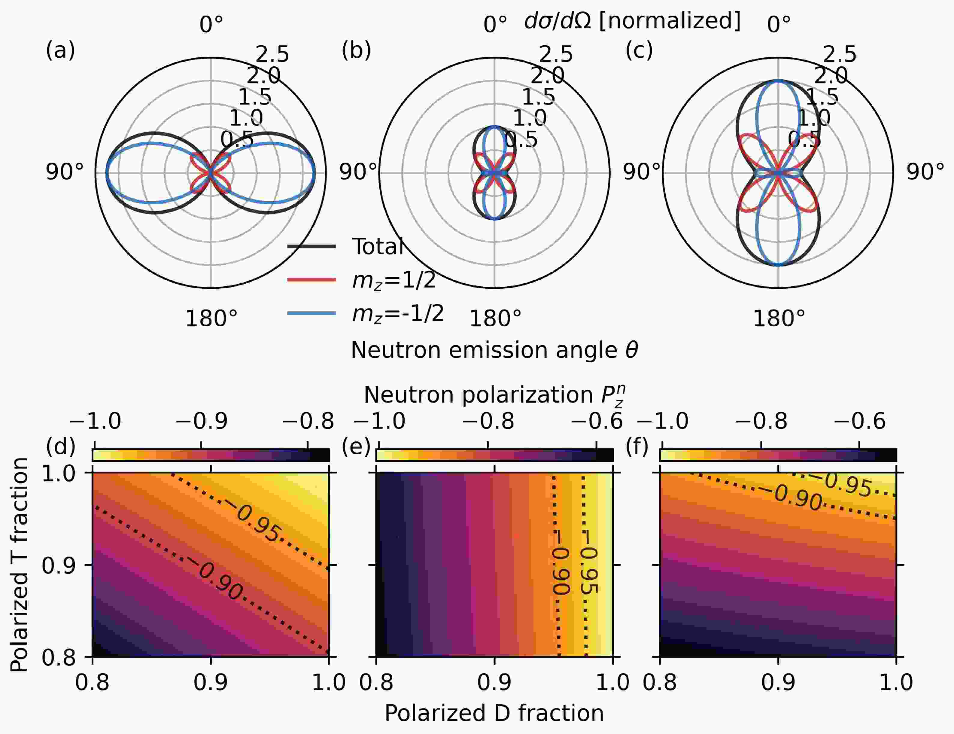
$ \dfrac{{\rm d}\sigma}{{\rm d}\Omega} $ ,$ \dfrac{{\rm d}\sigma}{{\rm d}\Omega}^+ $ ,$ \dfrac{{\rm d}\sigma}{{\rm d}\Omega}^- $ for tritons fully polarized in the$ m_z=1/2 $ state and deuterons polarized in the$ m_z=1 $ state (parallel polarization case). The polar angle of maximum neutron emission is$ \theta=90^\circ $ , and the maximum differential cross-section is 2.25 times the unpolarized differential cross-section$ \sigma_0/4\pi $ . The emitted neutrons near$ \theta=90^\circ $ are mostly in spin$ m_z=-1/2 $ state. When tritons are polarized in the$ m_z=1/2 $ state and deuterons are polarized in the$ m_z=-1 $ state (antiparallel polarization case), the polar angles of maximum neutron emission are$ \theta=0^\circ $ and$ \theta=180^\circ $ , as shown in Fig. 1(b). The maximum differential cross-section is equal to the unpolarized differential cross-section. The emitted neutrons near$ \theta=0^\circ $ and$ \theta=180^\circ $ are polarized in the$ m_z=-1/2 $ state. For tritons polarized in the$ m_z=-1/2 $ state and deuterons polarized in the$ m_z=0 $ state (perpendicular polarization case), the angular distributions are similar to those of the antiparallel polarization case, as depicted in Fig. 1(c). The maximum differential cross-section is 2 times the unpolarized one. In experiments, the DT fuels are not fully polarized, and the self-generated magnetic fields can lead to the depolarization of the fuel during the implosion. Equations (1) and (2) are used to obtain the neutron polarizations for different polarized deuteron and triton fractions. The neutron polarization is defined as the difference between neutron fractions in different spin states,$ p_z^n=n_{1/2}-n_{-1/2} $ , where$ n_{\pm1/2} $ are the fractions of neutrons in the$ m_z=\pm1/2 $ states, respectively. The neutron polarization at$ \theta=90^\circ $ for the parallel polarization case is shown in Fig. 1(d), and the neutron polarizations at$ \theta=0^\circ $ for the antiparallel and perpendicular polarization cases are shown in Figs. 1(e) and 1(f), respectively. The dashed lines in Figs. 1(e)−(f) show the boundaries of neutron polarization below –0.90 and –0.95. The parallel polarization case occupies larger areas of high neutron polarization in the parameter space than the antiparallel and perpendicular polarization cases, indicating higher tolerances for imperfect initial fuel polarization and depolarization.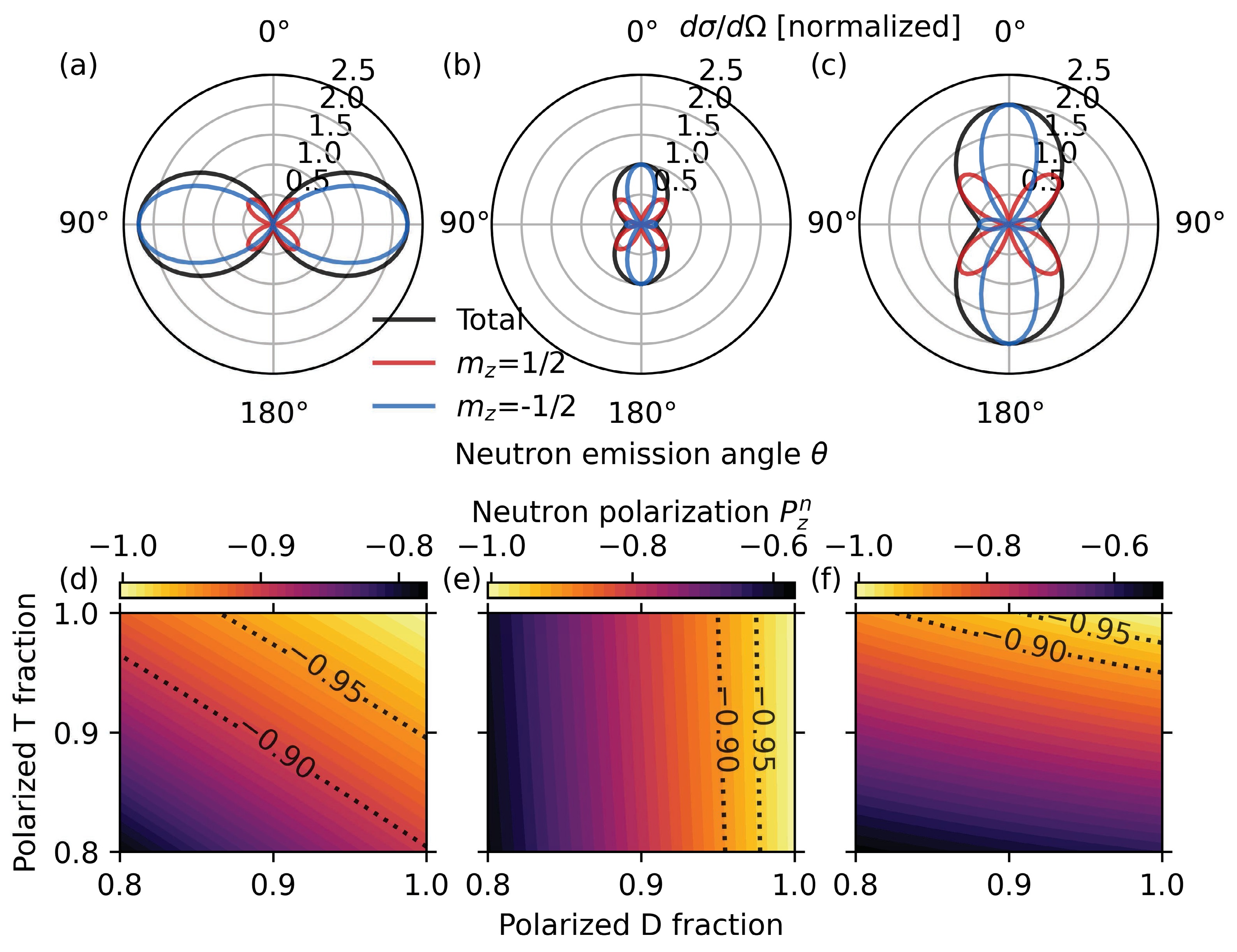
Figure 1. (color online) (a) Differential cross-sections for T in
$ m_z=1/2 $ state and D in$ m_z=1 $ state. (b) Differential cross-sections for T in$ m_z=1/2 $ state and D in$ m_z=-1 $ state. (c) Differential cross-sections for T in$ m_z=-1/2 $ state and D in$ m_z=0 $ state. (d) Neutron polarizations at$ \theta=90^\circ $ for different fractions of T in$ m_z=1/2 $ state and D in$ m_z=1 $ state. (e) Neutron polarizations at$ \theta=0^\circ $ for different fractions of T in$ m_z=1/2 $ state and D in$ m_z=-1 $ state. (f) Neutron polarizations at$ \theta=0^\circ $ for different fractions of T in$ m_z=-1/2 $ state and D in$ m_z=0 $ state. The differential cross-sections in (a)−(c) are normalized by the unpolarized total differential cross-section$ \sigma_0/4\pi $ . The fractions of D in the other two states are assumed to be equal in (d)−(f).To measure the path-integrated magnetic field strengths, three quantities are necessary: the total neutron fluence and the neutron fluences in one of the spin eigenstates with and without the magnetic field. These quantities vary from shot to shot, so single-shot measurements are required. In the case of parallel polarization, the polarized neutrons are emitted mostly at
$ \theta=90^\circ $ , and the distributions are almost uniform in terms of azimuthal angles, forming donut-like neutron beams. The required quantities can be measured at three different azimuthal angles simultaneously. The setup of the simulation is shown in Fig. 2. The capsule is filled with DT fuels in parallel polarization. Multiple lasers are used to drive the spherical implosion of the capsule, and donut-like neutron beams are generated. The magnetic fields are generated in laser-produced HED plasmas. The spin-filters, which allow neutrons in one eigenstate to pass through, are used to measure neutron fluences in one of the spin eigenstates. Three neutron detectors are placed at the same distance from the capsule with different azimuthal angles. The first neutron detector obtains the neutron fluences in one of the spin eigenstates after passing through the magnetic fields. The second neutron detector measures the neutron fluences in one of the spin eigenstates without magnetic fields. The third neutron detector measures the total neutron fluences.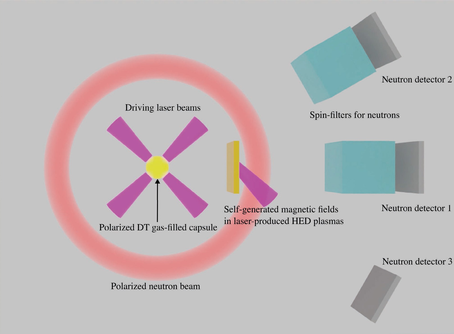
Figure 2. (color online) Top view of the simulation setup (not to scale).
-
The angular distribution of emitted neutrons can be predicted from the differential cross-section of the DT reaction [34, 35]:
$ \begin{aligned}[b] \frac{{\rm d}\sigma}{{\rm d} \Omega}\left(\theta, \phi\right)=\;&\frac{\sigma_0}{4\pi}\left[\frac{9}{4}\left(\eta^T_{00}\eta^D_{00}+\eta^T_{11}\eta^D_{22}\right)\sin^2\theta\right. \\ &\left.+\frac{1}{4}\left(\eta^T_{00}\eta^D_{22}+\eta^T_{11}\eta^D_{00}+2\eta^D_{11}\right)\left(3\cos^2\theta+1\right)\right], \end{aligned} $
(1) where θ is the polar angle, ϕ is the azimuthal angle, and
$ \sigma_0 $ is the unpolarized fusion cross-section.$ {\eta}^T_{00} $ and$ {\eta}^T_{11} $ are the diagonal terms of the spin density matrix of triton, indicating the probabilities of spin eigenstates$ m_z=\{\dfrac{1}{2},-\dfrac{1}{2}\} $ , respectively.$ {\eta}^D_{00} $ ,$ {\eta}^D_{11} $ , and$ {\eta}^D_{22} $ are the diagonal terms of the spin density matrix of deuteron, corresponding to the probabilities of spin eigenstates$ m_z=\{1,0,-1\} $ , respectively. The vector polarization of triton can be calculated as$ p_z^T=\eta_{00}^T-\eta_{11}^T $ . The vector polarization of deuteron is$ p_z^D=\eta_{00}^D-\eta_{22}^D $ , and the tensor polarization of deuteron is$ p_{zz}^D=\eta_{00}^D-2\eta_{11}^D+\eta_{22}^D $ . The differential cross-sections for neutrons in spin eigenstates$ m_z=\{\dfrac{1}{2},-\dfrac{1}{2}\} $ are$ \dfrac{{\rm d}\sigma}{{\rm d}\Omega}^+ $ and$ \dfrac{{\rm d}\sigma}{{\rm d}\Omega}^- $ , respectively, satisifying$ \dfrac{{\rm d}\sigma}{{\rm d}\Omega}=\dfrac{{\rm d}\sigma}{{\rm d}\Omega}^++\dfrac{{\rm d}\sigma}{{\rm d}\Omega}^- $ and$ \begin{aligned}[b] \frac{{\rm d}\sigma}{{\rm d}\Omega}^+-\frac{{\rm d}\sigma}{{\rm d}\Omega}^-=\;& \frac{\sigma_0}{4\pi}\left[\frac{9}{4}\left(\eta^T_{00}-\eta^T_{11}\right)\left(\eta^D_{00}-2\eta^D_{11}+\eta^D_{22}\right)\sin^2\theta\cos^2\theta\right.\\ &-\frac{9}{4}\left(\eta^T_{00}\eta^D_{00}-\eta^T_{11}\eta^D_{22}\right)\sin^4\theta+\frac{1}{4}\left(2\eta^T_{00}\eta^D_{11}\right.\\ &\left.\left.-2\eta^T_{11}\eta^D_{11}+\eta^T_{11}\eta^D_{00}-\eta^T_{00}\eta^D_{22}\right)\left(3\cos^2\theta-1\right)^2\right]. \end{aligned} $
(2) Figure 1(a) shows the differential cross-sections
$ \dfrac{{\rm d}\sigma}{{\rm d}\Omega} $ ,$ \dfrac{{\rm d}\sigma}{{\rm d}\Omega}^+ $ ,$ \dfrac{{\rm d}\sigma}{{\rm d}\Omega}^- $ for tritons fully polarized in the$ m_z=1/2 $ state and deuterons polarized in the$ m_z=1 $ state (parallel polarization case). The polar angle of maximum neutron emission is$ \theta=90^\circ $ , and the maximum differential cross-section is 2.25 times the unpolarized differential cross-section$ \sigma_0/4\pi $ . The emitted neutrons near$ \theta=90^\circ $ are mostly in spin$ m_z=-1/2 $ state. When tritons are polarized in the$ m_z=1/2 $ state and deuterons are polarized in the$ m_z=-1 $ state (antiparallel polarization case), the polar angles of maximum neutron emission are$ \theta=0^\circ $ and$ \theta=180^\circ $ , as shown in Fig. 1(b). The maximum differential cross-section is equal to the unpolarized differential cross-section. The emitted neutrons near$ \theta=0^\circ $ and$ \theta=180^\circ $ are polarized in the$ m_z=-1/2 $ state. For tritons polarized in the$ m_z=-1/2 $ state and deuterons polarized in the$ m_z=0 $ state (perpendicular polarization case), the angular distributions are similar to those of the antiparallel polarization case, as depicted in Fig. 1(c). The maximum differential cross-section is 2 times the unpolarized one. In experiments, the DT fuels are not fully polarized, and the self-generated magnetic fields can lead to the depolarization of the fuel during the implosion. Equations (1) and (2) are used to obtain the neutron polarizations for different polarized deuteron and triton fractions. The neutron polarization is defined as the difference between neutron fractions in different spin states,$ p_z^n=n_{1/2}-n_{-1/2} $ , where$ n_{\pm1/2} $ are the fractions of neutrons in the$ m_z=\pm1/2 $ states, respectively. The neutron polarization at$ \theta=90^\circ $ for the parallel polarization case is shown in Fig. 1(d), and the neutron polarizations at$ \theta=0^\circ $ for the antiparallel and perpendicular polarization cases are shown in Figs. 1(e) and 1(f), respectively. The dashed lines in Figs. 1(e)−(f) show the boundaries of neutron polarization below –0.90 and –0.95. The parallel polarization case occupies larger areas of high neutron polarization in the parameter space than the antiparallel and perpendicular polarization cases, indicating higher tolerances for imperfect initial fuel polarization and depolarization.
Figure 1. (color online) (a) Differential cross-sections for T in
$ m_z=1/2 $ state and D in$ m_z=1 $ state. (b) Differential cross-sections for T in$ m_z=1/2 $ state and D in$ m_z=-1 $ state. (c) Differential cross-sections for T in$ m_z=-1/2 $ state and D in$ m_z=0 $ state. (d) Neutron polarizations at$ \theta=90^\circ $ for different fractions of T in$ m_z=1/2 $ state and D in$ m_z=1 $ state. (e) Neutron polarizations at$ \theta=0^\circ $ for different fractions of T in$ m_z=1/2 $ state and D in$ m_z=-1 $ state. (f) Neutron polarizations at$ \theta=0^\circ $ for different fractions of T in$ m_z=-1/2 $ state and D in$ m_z=0 $ state. The differential cross-sections in (a)−(c) are normalized by the unpolarized total differential cross-section$ \sigma_0/4\pi $ . The fractions of D in the other two states are assumed to be equal in (d)−(f).To measure the path-integrated magnetic field strengths, three quantities are necessary: the total neutron fluence and the neutron fluences in one of the spin eigenstates with and without the magnetic field. These quantities vary from shot to shot, so single-shot measurements are required. In the case of parallel polarization, the polarized neutrons are emitted mostly at
$ \theta=90^\circ $ , and the distributions are almost uniform in terms of azimuthal angles, forming donut-like neutron beams. The required quantities can be measured at three different azimuthal angles simultaneously. The setup of the simulation is shown in Fig. 2. The capsule is filled with DT fuels in parallel polarization. Multiple lasers are used to drive the spherical implosion of the capsule, and donut-like neutron beams are generated. The magnetic fields are generated in laser-produced HED plasmas. The spin-filters, which allow neutrons in one eigenstate to pass through, are used to measure neutron fluences in one of the spin eigenstates. Three neutron detectors are placed at the same distance from the capsule with different azimuthal angles. The first neutron detector obtains the neutron fluences in one of the spin eigenstates after passing through the magnetic fields. The second neutron detector measures the neutron fluences in one of the spin eigenstates without magnetic fields. The third neutron detector measures the total neutron fluences.
Figure 2. (color online) Top view of the simulation setup (not to scale).
-
The STHD simulation code SPINSIM [4, 33] is used to obtain the spatial and angular distribution of the polarized neutron beams. Here, 3D simulations of directly driven implosions of the polarized DT gas-filled target are performed. The driving laser pulses have a total energy of 100 kJ and flat-top temporal profiles with pulse durations of 2 ns and rising and falling edges of 200 ps. The target capsule is filled with equimolar highly polarized DT gas with a density of 1 mg/cm
$ ^3 $ . The vector polarizations of tritons and vector and tensor polarizations of deuterons have a value of 0.9, which can be achieved with atomic beam sources. The fuel is encapsulated in a layer of high-density carbon ablator with a density of 3.52 g/cm$ ^3 $ . The inner radius of the capsule is 0.1 cm, and the thickness of the ablator is 5$ \mu $ m. One-dimensional radiation hydrodynamics code MULTI-IFE [37] is used to simulate the implosion dynamics of the capsule. The results of the MULTI-IFE simulations are used as the initial and boundary conditions of the stagnation phase simulations performed with the 3D SPINSIM code. The uniform computational mesh has a size of 512$ \times $ 512$ \times $ 512, and the simulation box is sized 600$ \times $ 600$ \times $ 600$ {\mu} $ m$ ^3 $ . The neutron emissivity, i.e., neutrons emitted per unit time and volume, is calculated as [33−35]$ \begin{aligned}[b] \varepsilon_n=\;&\left<\sigma_0 v\right>n_D^2\left[\frac{3}{2}\left(\eta^T_{00}\eta^D_{00}+\eta^T_{11}\eta^D_{22}\right)+\eta^D_{11}\right.\\ &\left.+\frac{1}{2}\left(\eta^T_{00}\eta^D_{22}+\eta^T_{11}\eta^D_{00}\right)\right], \end{aligned} $

(3) where
$ \left<\sigma_0 v\right> $ is the unpolarized DT fusion reactivity [38], and$ n_D $ is deuteron number density. The differential emissivity is$ \begin{aligned}[b] \frac{{\rm d} \varepsilon_n}{{\rm d} \Omega}=\;&\frac{\left<\sigma_0 v\right>}{4\pi}n_D^2\left[\frac{9}{4}\left(\eta^T_{00}\eta^D_{00}+\eta^T_{11}\eta^D_{22}\right)\sin^2\theta\right. \\ &\left.+\frac{1}{4}\left(\eta^T_{00}\eta^D_{22}+\eta^T_{11}\eta^D_{00}+2\eta^D_{11}\right)\left(3\cos^2\theta+1\right)\right]. \end{aligned} $

(4) The difference of differential emissivities of neutrons in spin up and down states is
$ \begin{aligned}[b] &\frac{{\rm d} \varepsilon_n^+}{{\rm d}\Omega}-\frac{{\rm d} \varepsilon_n^-}{{\rm d}\Omega}=\frac{\left<\sigma_0 v\right>}{4\pi}n_D^2\left[\frac{9}{4}\left(\eta^T_{00}-\eta^T_{11}\right)\left(\eta^D_{00}-2\eta^D_{11}+\eta^D_{22}\right)\right.\\ &\sin^2\theta\cos^2\theta-\frac{9}{4}\left(\eta^T_{00}\eta^D_{00}-\eta^T_{11}\eta^D_{22}\right)\sin^4\theta+\frac{1}{4}\left(2\eta^T_{00}\eta^D_{11}\right.\\ &\left.\left.-2\eta^T_{11}\eta^D_{11}+\eta^T_{11}\eta^D_{00}-\eta^T_{00}\eta^D_{22}\right)\left(3\cos^2\theta-1\right)^2\right], \end{aligned} $

(5) $ \dfrac{{\rm d} \varepsilon_n^+}{{\rm d}\Omega} $ and$ \dfrac{{\rm d} \varepsilon_n^-}{{\rm d}\Omega} $ are the differential emissivities for neutrons in the$ m_z=\{\dfrac{1}{2},-\dfrac{1}{2}\} $ states, respectively. Six 3D arrays are used in SPINSIM to store the data of time-integrated neutron emissivity and differential emissivities. One is used to store the time-integrated neutron emissivity. Two are used to store the time-integrated coefficients of the$ \sin^2\theta $ and$ \left(3\cos^2\theta+1\right) $ terms in Eq. (4). The remaining three are used to store the time-integrated coefficients of the$ \sin^2\theta\cos^2\theta $ ,$ \sin^4\theta $ , and$ \left(3\cos^2\theta-1\right)^2 $ terms in Eq. (5).Figure 3(a) shows the 3D spatial distribution of the time-integrated neutron emissivity obtained from the SPINSIM simulation. The total neutron yield, obtained by integrating the emissivity over time and space, is 3.31
$ \times $ 10$ ^{15} $ . The time-integrated neutron emissivity on the$ x=0 $ plane is shown in Fig. 3(b), and the full width at half maximum (FWHM) of the source is 80$ \mu $ m. The mass density distribution on the$ x=0 $ plane at maximum compression is depicted in Fig. 3(c). The low-density region in the center is the compressed fuel, which forms the hot spot, and the high-density shell surrounding the hot spot is formed by the remaining carbon ablator. Neutrons are generated inside the hot spot, and their spatial distribution, with a small spike in the center, is different from the Gaussian distribution. The shape of the neutron source is affected by the shape of the hot spot, which is influenced by the Rayleigh-Taylor instability near the fuel-shell interface.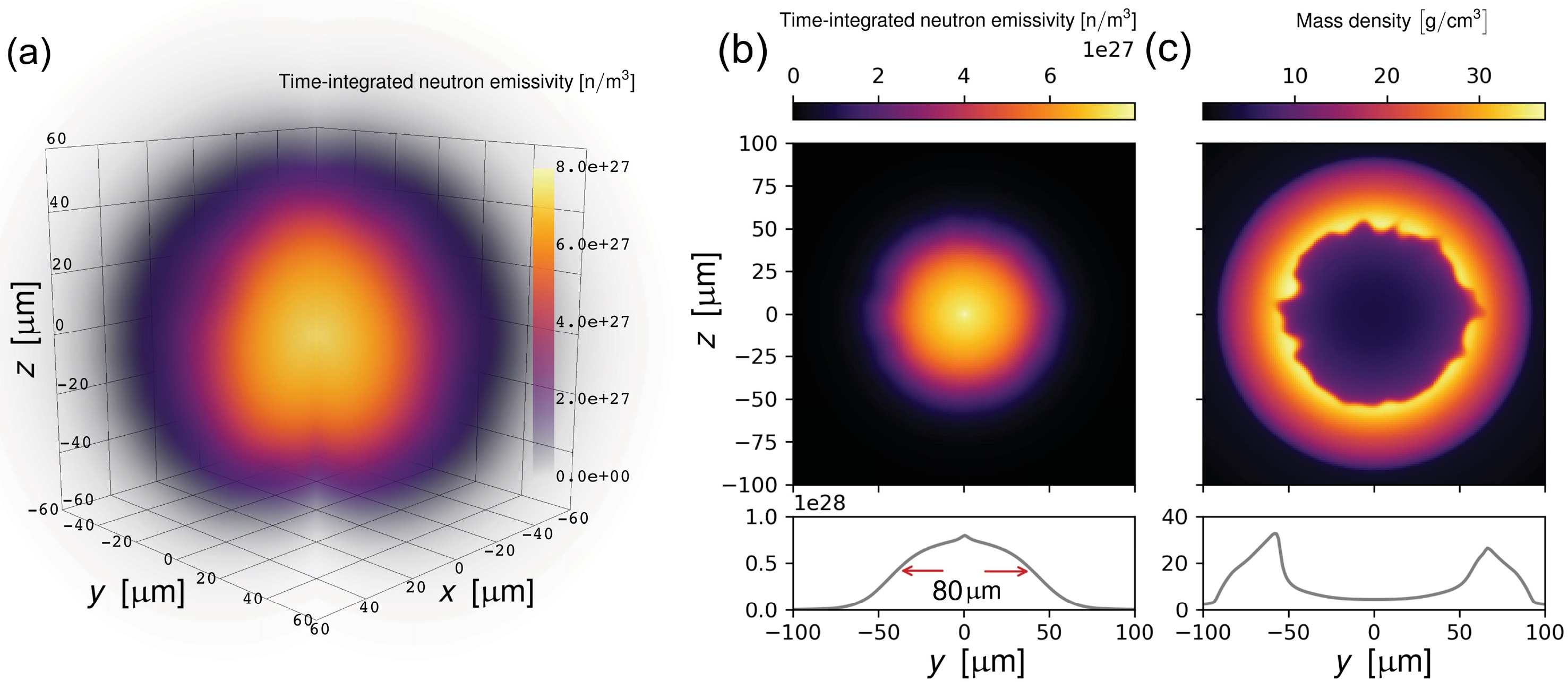
Figure 3. (color online) (a) 3D distribution of the time-integrated neutron emissivity; the data in
$ x,y>0 $ region are set to be transparent to visualize the data in the center. (b) 2D distribution of the time-integrated neutron emissivity at the x=0 plane. (c) 2D distribution of the mass density at the maximum compression. The lower panels in (b) and (c) show the 1D distributions along the y-axis.The differential yields can also be obtained from SPINSIM simulations including the DT depolarization effects. The differential yield for the parallel polarization case is shown in Fig. 4(a). The initial vector polarization for T and vector and tensor polarizations for D are all set as 0.9. Neglecting the DT depolarization during the implosion, the theoretical neutron polarization given by Eqs. (1) and (2) is
$ -0.969 $ . Similar to the differential cross-sections in Fig. 1(a), the differential yields also indicate that the neutrons are polarized in the θ=90$ ^\circ $ direction. The peak neutron differential yield is 3.81$ \times $ 10$ ^{14} $ n/sr, and the neutron polarization at θ=90$ ^\circ $ is$ -0.968 $ . For the anti-parallel polarization case, the initial vector polarization for T is 0.9, the vector polarization for D is$ -0.9 $ , and the tensor polarization for D is 0.9. The theoretical neutron polarization is$ -0.864 $ . As shown in Fig. 4(b), the peak neutron differential yield is 1.79$ \times $ 10$ ^{14} $ n/sr, and the neutron polarization at θ=0$ ^\circ $ is$ -0.863 $ . For the perpendicular polarization case, the initial vector polarization for T is$ -0.9 $ , the vector polarization for D is 0, and the tensor polarization for D is$ -1.8 $ . The theoretical neutron polarization is given as$ -0.868 $ . The peak neutron differential yield is 3.57$ \times $ 10$ ^{14} $ n/sr, and the neutron polarization at θ=0$ ^\circ $ is$ -0.863 $ . Only the initial polarizations of the DT fuels are changed for different cases, and other simulation parameters are unchanged. The parallel polarization case has the largest peak neutron differential yield and absolute neutron polarization. For the anti-parallel and perpendicular polarization cases, the peak differential yields and neutron polarizations are obtained at θ=0$ ^\circ $ and θ=180$ ^\circ $ , so it is not feasible to measure the neutron fluences at three different angles in a single shot.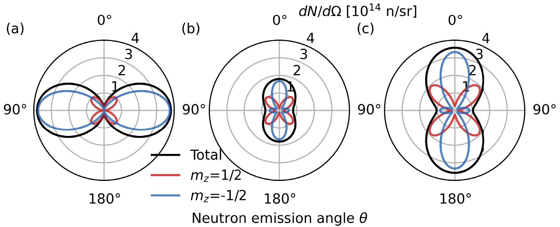
Figure 4. (color online) Neutron differential yields for the (a) parallel, (b) anti-parallel, and (c) perpendicular polarization cases.
-
The STHD simulation code SPINSIM [4, 33] is used to obtain the spatial and angular distribution of the polarized neutron beams. Here, 3D simulations of directly driven implosions of the polarized DT gas-filled target are performed. The driving laser pulses have a total energy of 100 kJ and flat-top temporal profiles with pulse durations of 2 ns and rising and falling edges of 200 ps. The target capsule is filled with equimolar highly polarized DT gas with a density of 1 mg/cm
$ ^3 $ . The vector polarizations of tritons and vector and tensor polarizations of deuterons have a value of 0.9, which can be achieved with atomic beam sources. The fuel is encapsulated in a layer of high-density carbon ablator with a density of 3.52 g/cm$ ^3 $ . The inner radius of the capsule is 0.1 cm, and the thickness of the ablator is 5$ \mu $ m. One-dimensional radiation hydrodynamics code MULTI-IFE [37] is used to simulate the implosion dynamics of the capsule. The results of the MULTI-IFE simulations are used as the initial and boundary conditions of the stagnation phase simulations performed with the 3D SPINSIM code. The uniform computational mesh has a size of 512$ \times $ 512$ \times $ 512, and the simulation box is sized 600$ \times $ 600$ \times $ 600$ {\mu} $ m$ ^3 $ . The neutron emissivity, i.e., neutrons emitted per unit time and volume, is calculated as [33−35]$ \begin{aligned}[b] \varepsilon_n=\;&\left<\sigma_0 v\right>n_D^2\left[\frac{3}{2}\left(\eta^T_{00}\eta^D_{00}+\eta^T_{11}\eta^D_{22}\right)+\eta^D_{11}\right.\\ &\left.+\frac{1}{2}\left(\eta^T_{00}\eta^D_{22}+\eta^T_{11}\eta^D_{00}\right)\right], \end{aligned} $
(3) where
$ \left<\sigma_0 v\right> $ is the unpolarized DT fusion reactivity [38], and$ n_D $ is deuteron number density. The differential emissivity is$ \begin{aligned}[b] \frac{{\rm d} \varepsilon_n}{{\rm d} \Omega}=\;&\frac{\left<\sigma_0 v\right>}{4\pi}n_D^2\left[\frac{9}{4}\left(\eta^T_{00}\eta^D_{00}+\eta^T_{11}\eta^D_{22}\right)\sin^2\theta\right. \\ &\left.+\frac{1}{4}\left(\eta^T_{00}\eta^D_{22}+\eta^T_{11}\eta^D_{00}+2\eta^D_{11}\right)\left(3\cos^2\theta+1\right)\right]. \end{aligned} $
(4) The difference of differential emissivities of neutrons in spin up and down states is
$ \begin{aligned}[b] &\frac{{\rm d} \varepsilon_n^+}{{\rm d}\Omega}-\frac{{\rm d} \varepsilon_n^-}{{\rm d}\Omega}=\frac{\left<\sigma_0 v\right>}{4\pi}n_D^2\left[\frac{9}{4}\left(\eta^T_{00}-\eta^T_{11}\right)\left(\eta^D_{00}-2\eta^D_{11}+\eta^D_{22}\right)\right.\\ &\sin^2\theta\cos^2\theta-\frac{9}{4}\left(\eta^T_{00}\eta^D_{00}-\eta^T_{11}\eta^D_{22}\right)\sin^4\theta+\frac{1}{4}\left(2\eta^T_{00}\eta^D_{11}\right.\\ &\left.\left.-2\eta^T_{11}\eta^D_{11}+\eta^T_{11}\eta^D_{00}-\eta^T_{00}\eta^D_{22}\right)\left(3\cos^2\theta-1\right)^2\right], \end{aligned} $
(5) $ \dfrac{{\rm d} \varepsilon_n^+}{{\rm d}\Omega} $ and$ \dfrac{{\rm d} \varepsilon_n^-}{{\rm d}\Omega} $ are the differential emissivities for neutrons in the$ m_z=\{\dfrac{1}{2},-\dfrac{1}{2}\} $ states, respectively. Six 3D arrays are used in SPINSIM to store the data of time-integrated neutron emissivity and differential emissivities. One is used to store the time-integrated neutron emissivity. Two are used to store the time-integrated coefficients of the$ \sin^2\theta $ and$ \left(3\cos^2\theta+1\right) $ terms in Eq. (4). The remaining three are used to store the time-integrated coefficients of the$ \sin^2\theta\cos^2\theta $ ,$ \sin^4\theta $ , and$ \left(3\cos^2\theta-1\right)^2 $ terms in Eq. (5).Figure 3(a) shows the 3D spatial distribution of the time-integrated neutron emissivity obtained from the SPINSIM simulation. The total neutron yield, obtained by integrating the emissivity over time and space, is 3.31
$ \times $ 10$ ^{15} $ . The time-integrated neutron emissivity on the$ x=0 $ plane is shown in Fig. 3(b), and the full width at half maximum (FWHM) of the source is 80$ \mu $ m. The mass density distribution on the$ x=0 $ plane at maximum compression is depicted in Fig. 3(c). The low-density region in the center is the compressed fuel, which forms the hot spot, and the high-density shell surrounding the hot spot is formed by the remaining carbon ablator. Neutrons are generated inside the hot spot, and their spatial distribution, with a small spike in the center, is different from the Gaussian distribution. The shape of the neutron source is affected by the shape of the hot spot, which is influenced by the Rayleigh-Taylor instability near the fuel-shell interface.
Figure 3. (color online) (a) 3D distribution of the time-integrated neutron emissivity; the data in
$ x,y>0 $ region are set to be transparent to visualize the data in the center. (b) 2D distribution of the time-integrated neutron emissivity at the x=0 plane. (c) 2D distribution of the mass density at the maximum compression. The lower panels in (b) and (c) show the 1D distributions along the y-axis.The differential yields can also be obtained from SPINSIM simulations including the DT depolarization effects. The differential yield for the parallel polarization case is shown in Fig. 4(a). The initial vector polarization for T and vector and tensor polarizations for D are all set as 0.9. Neglecting the DT depolarization during the implosion, the theoretical neutron polarization given by Eqs. (1) and (2) is
$ -0.969 $ . Similar to the differential cross-sections in Fig. 1(a), the differential yields also indicate that the neutrons are polarized in the θ=90$ ^\circ $ direction. The peak neutron differential yield is 3.81$ \times $ 10$ ^{14} $ n/sr, and the neutron polarization at θ=90$ ^\circ $ is$ -0.968 $ . For the anti-parallel polarization case, the initial vector polarization for T is 0.9, the vector polarization for D is$ -0.9 $ , and the tensor polarization for D is 0.9. The theoretical neutron polarization is$ -0.864 $ . As shown in Fig. 4(b), the peak neutron differential yield is 1.79$ \times $ 10$ ^{14} $ n/sr, and the neutron polarization at θ=0$ ^\circ $ is$ -0.863 $ . For the perpendicular polarization case, the initial vector polarization for T is$ -0.9 $ , the vector polarization for D is 0, and the tensor polarization for D is$ -1.8 $ . The theoretical neutron polarization is given as$ -0.868 $ . The peak neutron differential yield is 3.57$ \times $ 10$ ^{14} $ n/sr, and the neutron polarization at θ=0$ ^\circ $ is$ -0.863 $ . Only the initial polarizations of the DT fuels are changed for different cases, and other simulation parameters are unchanged. The parallel polarization case has the largest peak neutron differential yield and absolute neutron polarization. For the anti-parallel and perpendicular polarization cases, the peak differential yields and neutron polarizations are obtained at θ=0$ ^\circ $ and θ=180$ ^\circ $ , so it is not feasible to measure the neutron fluences at three different angles in a single shot.
Figure 4. (color online) Neutron differential yields for the (a) parallel, (b) anti-parallel, and (c) perpendicular polarization cases.
-
Monte Carlo simulations are used to investigate the polarized neutron imaging of magnetic fields with the polarized neutron source from the imploded capsule. The macro-particle representing neutrons is initialized with random positions according to the emissivity distribution shown in Fig. 3(a). The energies of the neutrons are 14.1 MeV, and the velocity directions are sampled from the angular distribution given by the SPINSIM simulation. As mentioned in Sec. III, the spatial and angular distributions of the neutron source are stored in six 3D arrays. As only the static magnetic field imaging is investigated in this study, the temporal effects are not considered. To investigate temporal effects, 4D arrays should be used to include the temporal variations of the neutron source. The coordinates of a computational cell
$ (i,j,k) $ are$ (x_{i,j,k}, \ y_{i,j,k},\ z_{i,j,k}) $ , and the neutron yield in the cell is$ N_{i,j,k} $ . The differential yields in each cell are$ \begin{aligned}[b] \frac{{\rm d}}{N_{i,j,k}}{{\rm d}\Omega}=\; &\frac{{\rm d}N_{i,j,k}^+}{{\rm d}\Omega}+\frac{{\rm d}N_{i,j,k}^-}{{\rm d}\Omega}\\ =\; &{C_1}_{i,j,k}\sin^2\theta+{C_2}_{i,j,k}\left(3\cos^2\theta+1\right),\\ \frac{{\rm d}N_{i,j,k}^+}{{\rm d}\Omega}-\frac{{\rm d}N_{i,j,k}^-}{{\rm d}\Omega}=\; &{C_3}_{i,j,k}\sin^2\theta \cos^2\theta\\ & +{C_4}_{i,j,k}\sin^4\theta+{C_5}_{i,j,k}\left(3\cos^2\theta-1\right)^2, \end{aligned} $

(6) where
$ \dfrac{{\rm d}N}{{\rm d}\Omega} $ is the total differential yield,$ \dfrac{{\rm d}N^\pm}{{\rm d}\Omega} $ are the differential yields for$ m_z=\pm\dfrac{1}{2} $ states, respectively, and$ C_1 $ -$ C_5 $ are the coefficients calculated from Eqs. (4) and (5). The random spatial and velocity distributions of macro-particles are generated from the six 3D arrays N and$ C_1 $ -$ C_5 $ with the inverse cumulative distribution function (CDF) method. The 3D arrays are flattened into 1D arrays by introducing a new index$ l=iN_yN_z+jN_z+k $ , where$ N_x $ ,$ N_y $ ,$ N_z $ are the numbers of grid cells in x, y, and z directions, respectively. The discretized CDF of the spatial distribution can be calculated as$ \begin{aligned} F_l = \sum_0^l N_l/\sum_0^{N_xN_yN_z} N_l. \end{aligned} $

(7) For each particle, a random number
$ p_0 $ is generated from the uniform distribution$ [0,1) $ , and the cell index of the particle is determined by$ F_{l-1}\leq p_0 <F_l $ . The particle coordinate can be calculated as$ \begin{aligned} x = x_l + p_1 {\rm d}x,\ y = y_l + p_2 {\rm d}y,\ z = z_l + p_3 {\rm d}z, \end{aligned} $

(8) where
$ p_1 $ -$ p_3 $ are random numbers from the uniform distribution$ [0,1) $ .$ {\rm d}x $ ,$ {\rm d}y $ , and$ {\rm d}z $ are the cell sizes. The CDF of the angular distribution is$ \begin{aligned}[b] G_l(\theta)=\;&\frac{\int_0^{\pi/2-\theta_m}\left({C_1}_l\sin^2\theta+{C_2}_l\left(3\cos^2\theta+1\right)\right)\sin\theta {\rm d}\theta}{\int_{\pi/2-\theta_m}^{\pi/2+\theta_m}\left({C_1}_l\sin^2\theta+{C_2}_l\left(3\cos^2\theta+1\right)\right)\sin\theta {\rm d}\theta}\\ &\begin{aligned}=[(&{C_2}_l-{C_1}_l/3)(\sin^3\theta_m-\cos^3\theta)+\\ (&{C_2}_l+{C_1}_l)(\sin\theta_m-\cos\theta)]/\\ [(&{C_2}_l-{C_1}_l/3)(2\sin^3\theta_m)+({C_2}_l+{C_1}_l)(2\sin\theta_m)].\end{aligned} \end{aligned} $

(9) Neutrons with divergence angles larger than
$ \theta_m= \arctan((L_z/2+z_{\rm max})/(x_s-x_{\rm max})) $ are located outside the detector, so they are neglected in the simulation to reduce computational cost.$ L_z $ is the detector length in the z direction, while$ x_s $ is the x coordinate of the detector, and$ x_{\rm max} $ and$ z_{\rm max} $ are the largest neutron coordinates in the x and z directions, respectively. By solving the equation$ G_l(\theta)=p_4 $ , one can obtain the polar angle θ for the macro-particle, where$ p_4 $ is from the uniform distribution$ [0,1) $ . The azimuthal angle is obtained by$ \phi=(2p_5-1)\phi_m $ , where$ p_5 $ is also from the uniform distribution$ [0,1) $ ,$ \phi_m= \arctan((L_y/2+y_{\rm max})/(x_s-x_{\rm max})) $ .$ (\theta,\phi) $ determines the velocity direction of the macro-particle. The macro-particle used in the simulation represents a statistical ensemble of numerous real particles. The number of such particles determines the weight of the macro-particle. The weight of a macro-particle is calculated as$ \begin{aligned} w=\frac{4\phi_m}{N_p}\left[({C_2}_l-{C_1}_l/3)\sin^3\theta_m+({C_2}_l+{C_1}_l)\sin\theta_m\right], \end{aligned} $

(10) where
$ N_p $ is the total number of macro-particles. The neutron spin states can be described by the spin vector. The spin states of the macro-particle are described by the ensemble average of spin vectors$ \left<{\boldsymbol{s}}\right>=(\left<s_x\right>, \left<s_y\right>, \left<s_z\right>) $ . The azimuthal angles of spin vectors are random, so$ \left<s_x\right> $ and$ \left<s_y\right> $ are both zero.$ \left<s_z\right> $ is calculated as$ \begin{aligned} \left<s_z\right>=\frac{{C_3}_l\sin^2\theta \cos^2\theta+{C_4}_l\sin^4\theta+{C_5}_l\left(3\cos^2\theta-1\right)^2}{{C_1}_l\sin^2\theta+{C_2}_l\left(3\cos^2\theta+1\right)}. \end{aligned} $

(11) The spin precession of the macro-particle in magnetic fields can be described by [25]
$ \begin{aligned} \frac{{\rm d}\left<{\boldsymbol{s}}\right>}{{\rm d}t}=\gamma_n\left<{\boldsymbol{s}}\right>\times{\boldsymbol{B}}, \end{aligned} $

(12) where
$ \gamma_n $ =$ -1.83\times10^8 $ $ \text{rad}/(\text{s}\cdot \text{T}) $ is the gyromagnetic ratio of a neutron, and$ {\boldsymbol{B}} $ is the magnetic field vector. For constant magnetic fields, Eq. (12) can be solved analytically. The spin vector rotates around the magnetic field with a constant frequency$ \omega_L=\gamma_n|B| $ , known as the Larmor frequency. To solve Eq. (12) for a time-varying magnetic field, the discrete time step$ {\rm d}t $ should be sufficiently small, and the magnetic field is assumed to be constant within each time step. At each time step, the analytical solution is used to advance the spin precession. For a magnetic field rotating around the x-axis with a frequency of$ \omega_B $ and constant strength of 1 T, the numerical solutions obtained for different time step sizes are compared with the analytical solution in adiabatic approximation, as shown in Fig. 5. The adiabatic approximation assumes that the spin vector locally precesses around the instant direction of the magnetic field, which is valid when$ \omega_B\ll \omega_L $ . For$ \omega_B=0.1\omega_L $ , our numerical solutions agree well with the adiabatic solution, as shown in Fig. 5(a). For$ \omega_B=0.7\omega_L $ , the adiabatic approximation is no longer valid, as evidenced by the discrepancy between the adiabatic solution and our numerical solution, as illustrated in Fig. 5(b). Because we use the analytical solution to advance the spin precession, the time step$ {\rm d}t $ does not need to be significantly smaller than the Larmor period$ T_L=2\pi/\omega_L $ , as in the finite difference method. The time step$ {\rm d}t $ only needs to be much smaller than the characteristic time scale of the varying magnetic field; in this case, the period of rotation$ T_B=2\pi/\omega_B $ . For$ {\rm d}t=T_B/40 $ , our numerical solution can already give consistent results with a highly resolved solution, as shown in Figs. 5(a) and 5(b).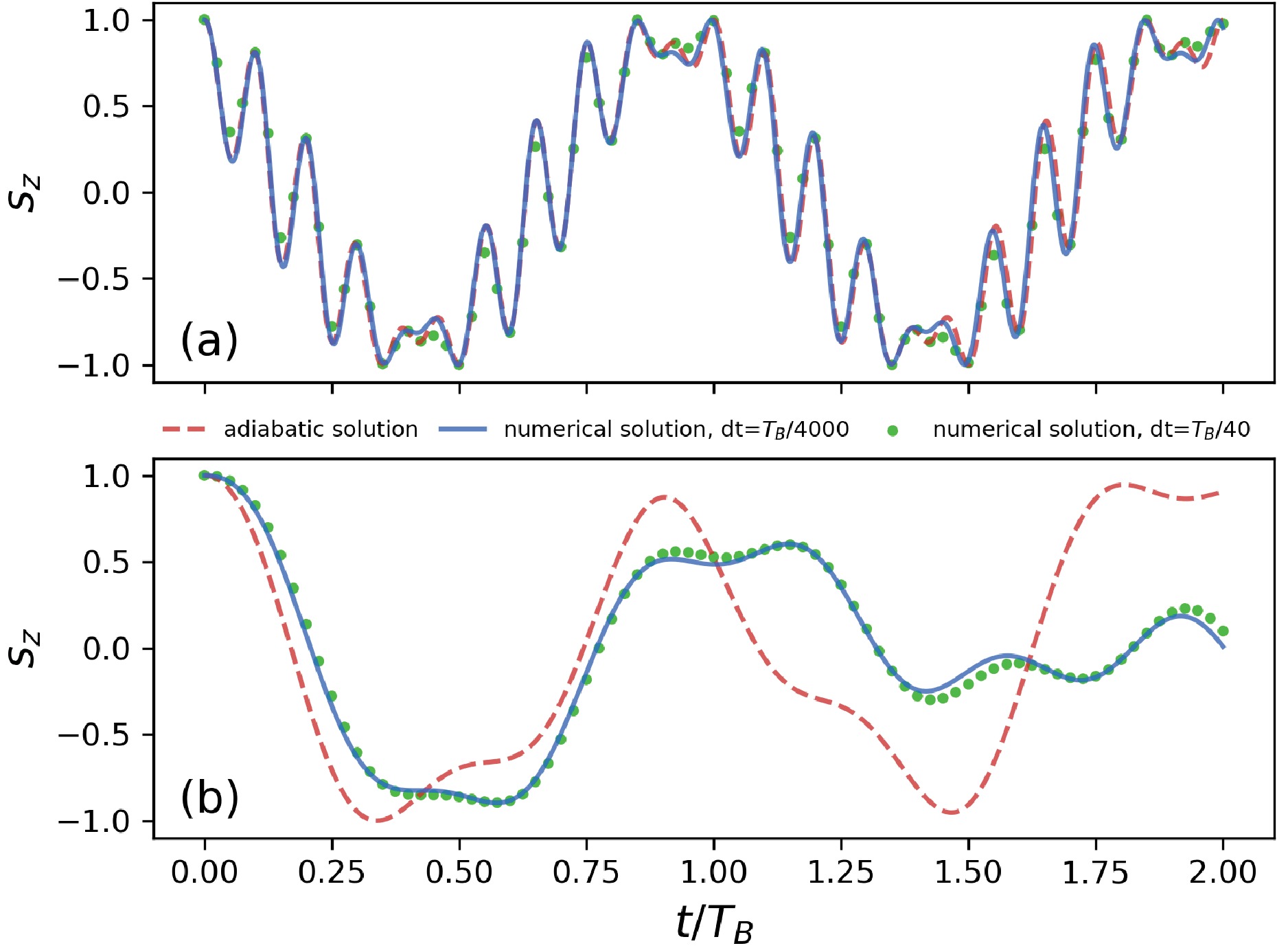
Figure 5. (color online) Comparison of the analytical solution in adiabatic approximation and numerical solutions with different time step sizes
$ {\rm d}t $ of the spin precession Eq. (12). The z component of the spin vector$ \left<s\right> $ is shown. The magnetic field rotates around the x-axis with (a)$ \omega_B=0.1\omega_L $ , (b)$ \omega_B=0.7\omega_L $ , where$ \omega_B $ is the angular frequency of the rotating magnetic field,$ \omega_L $ is the Larmor frequency, and$ T_B=2\pi/\omega_B $ is the rotation period of the magnetic field.The magnetic field used in the Monte Carlo simulation is given by
$ \begin{aligned} B_y = B_0\exp\left(-(x-x_0)^2/w_x^2\right)\cos\left(2\pi z/\lambda_z+\psi\right). \end{aligned} $

(13) The magnetic field has only a y component. The neutron beam propagates along the
$ +x $ direction (longitudinal direction), and the neutron polarization is along the z direction.$ B_0 $ is the peak magnetic field strength. In addition,$ x_0 $ is the longitudinal center of the magnetic field, and$ w_x $ is the longitudinal width of the magnetic field. In the simulation, magnetic field strength and longitudinal width are chosen close to the laser-driven HED conditions, with$ B_0=5000 $ T and$ w_x=50\ \mu\text{m} $ . The magnetic field is periodic along the z direction with a wavelength of$ \lambda_z $ and phase of ψ. The neutron source is placed at the origin. The magnetic field center is at$ x_0=2 $ cm, and three neutron detectors are placed at 1 m from the source. Macro-particles move from their initial positions to the detectors in straight lines. The evolution of the spin vector in magnetic field is calculated for each macro-particle. The time step size used to solve spin precession (Eq. (12)) is$ {\rm d}t=w_x/(51.2v_n) $ , where$ v_n $ is the neutron velocity. The counts of the macro-particles are added to the detectors, which have dimensions of 10×10 cm and a pixel resolution of 200×200. The neutron source is a point-like source with small source sizes, and the geometric magnification of the detector image is 50. The first neutron detector measures the neutron fluence$ F_1(y,z) $ of the spin down state after passing through the magnetic field. The second neutron detector measures the neutron fluence$ F_2(y,z) $ of the spin down state without passing through the magnetic field. The third neutron detector measures the neutron fluence$ F_3(y,z) $ of both the spin up and down states. The initial neutron polarization can be calculated as$ P_{z0}^n(y,z)=1-2F_2/F_3 $ , and the neutron polarization after passing through the magnetic field is$ P_z^n(y,z)= 1-2F_1/F_3 $ . For an ideal point source, the path-integrated magnetic field strength can be given by$ \begin{aligned} \left|\int B_y {\rm d}s\right| = \frac{v_n}{\gamma_n}\left(\pi-\arccos(P_z^n/\left|P_{z0}^n\right|)\right). \end{aligned} $

(14) For a finite-size source, neutrons from different source positions experience different magnetic fields and then meet at the detector. To obtain the path-integrated magnetic field strength using finite-size sources, a deblurring algorithm is proposed, which is discussed in the following section.
The polarizations of neutrons from different sources after passing through the magnetic field are depicted in Fig. 6. Figure 6(a) shows the results of neutrons from an ideal point source, with an initial neutron polarization of
$ -1 $ , passing through magnetic fields with a wavelength$ \lambda_z=200\ \mu\text{m} $ . The neutron polarization distributions are modulated by the periodic magnetic field. The modulation wavelength of the detector image is 0.5 cm, corresponding to a magnetic field strength variation wavelength of 100$ \mu\text{m} $ due to a geometric magnification of 50. As shown in Eq. (14), the polarized neutron imaging can only measure the absolute strength of the magnetic field. The variation wavelength of the magnetic field strength$ |B| $ is$ \lambda_z/2 $ . The neutron polarization image of a Gaussian source with an FWHM of 80$ \mu\text{m} $ and initial neutron polarization of$ -1 $ is shown in Fig. 6(b). The amplitude of the polarization modulation in this case is smaller than that in the point source case due to the finite-size-source blurring effect. The amplitude of the polarization modulation for the imploded-capsule source is also smaller than that of the point source case, as shown in Fig. 6(c). For the ideal point source, the spatial resolution is limited only by the resolution and signal-to-noise ratio of the detector. With sufficiently high detector resolution and signal-to-noise ratio, the 50$ \mu\text{m} $ wavelength corresponding to the magnetic field strength variation can be resolved by the ideal point source, as illustrated in Fig. 6(d). However, for the Gaussian source and the imploded-capsule source, both with an FWHM of 80$ \mu\text{m} $ , the 50$ \mu\text{m} $ variation wavelength can barely be resolved even when the detector resolution and signal-to-noise ratio are sufficiently high, as shown in Figs. 6(e) and 6(f).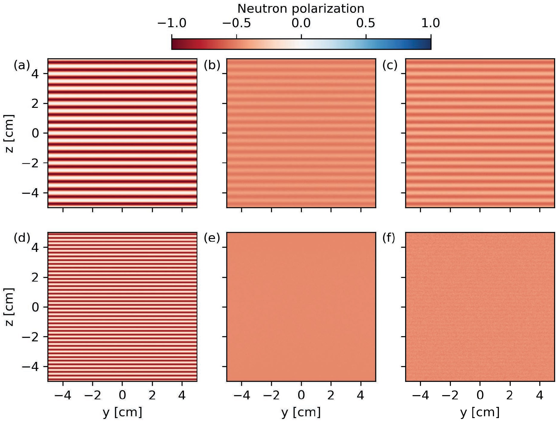
Figure 6. (color online) Neutron polarization distributions after passing through the magnetic field. (a) Point source and magnetic field strength variation wavelength of 100
$ \mu\text{m} $ . (b) Gaussian source with FWHM of 80$ \mu\text{m} $ and magnetic field strength variation wavelength of 100$ \mu\text{m} $ . (c) Imploded-capsule source with FWHM of 80$ \mu\text{m} $ and magnetic field strength variation wavelength of 100$ \mu\text{m} $ . (d) Point source and magnetic field strength variation wavelength of 50$ \mu\text{m} $ . (e) Gaussian source with FWHM of 80$ \mu\text{m} $ and magnetic field strength variation wavelength of 50$ \mu\text{m} $ . (f) Imploded-capsule source with FWHM of 80$ \mu\text{m} $ and magnetic field strength variation wavelength of 50$ \mu\text{m} $ .Using the neutron polarizations of the finite-size source in Eq. (14) will lead to an incorrect path-integrated magnetic field strength. The decrements in the neutron polarization modulations of the finite-size sources are quantitively calculated and shown in Fig. 7. The discrete Fourier transforms (DFTs) of the neutron polarization distributions along the y-axis are shown in Fig. 7(a). The wavelength corresponding to the magnetic field strength variation is
$ 100\ \mu\text{m} $ , and the first-order peaks of the spectra are located at 0.01$ \mu\text{m}^{-1} $ . In the point source case, the spectrum has multiple peaks, indicating high-order components. For the imploded-capsule source, due to the finite-source-size blurring, the amplitude of the first-order peak is smaller than that of the point source case, and the high-order components are missing. The spectral loss rate is defined as the ratio of amplitudes of the first-order peaks of the finite-size source and point source. The spectral loss rates of different sources as functions of the magnetic field strength variation wavelength are shown in Fig. 7(b). The spectral loss rate increases with the characteristic wavelength and decreases with the source size. An empirical formula for the spectral loss rate is obtained by fitting the simulation results, which can be written as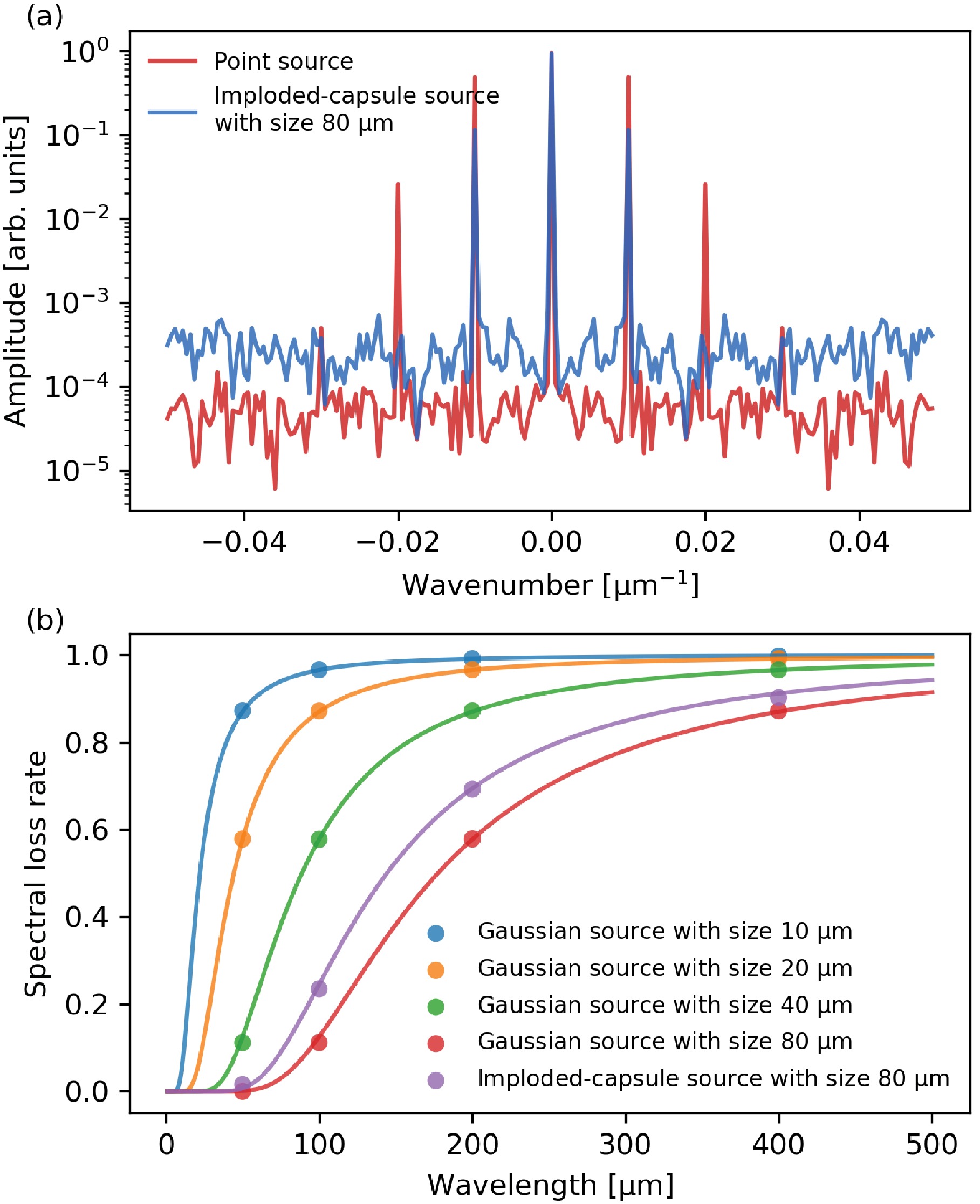
Figure 7. (color online) (a) DFT spectra of the neutron polarization distributions along the y-axis for the point source and imploded-capsule source. (b) Spectral loss rates as functions of the characteristic wavelengths for Gaussian sources with different source sizes and the imploded-capsule source. The circles denote the Monte Carlo simulation results, and solid lines are curves fitted using Eq. (15).
$ \begin{aligned} L(\lambda)=\frac{1}{\left[1+\left(s/2\lambda\right)^2\right]^{14}}, \end{aligned} $

(15) where
$ L(\lambda) $ is the spectral loss rate, λ is the characteristic wavelength, and s is the fitting parameter. The results of the fitting are illustrated as solid curves in Fig. 7(b). For Gaussian sources, it is found that s is equal to the FWHM of the source. For the imploded-capsule source with an FWHM of 80$ \mu\text{m} $ , s is equal to 65$ \mu\text{m} $ .By employing the spectral loss rate, the decrement in the amplitude of neutron polarization variation can be compensated. The compensated neutron polarization distribution can be written as
$ \begin{aligned} P_z^{n*}=\text{Re}\left\{{\cal{F}}^{-1}_y\left\{{\cal{F}}_y\left\{P_z^n\right\}/L(\lambda)\right\}\right\}, \end{aligned} $

(16) where
$ {\cal{F}}_y $ is the Fourier transform in the y direction, and$ {\cal{F}}_y^{-1} $ is the inverse Fourier transform. Equation (16) is the general expression used for the spectral amplitude compensation. In practice,$ L(\lambda) $ is manually set to 1 for$ \lambda<s $ to avoid the amplification of high-frequency noise. The values of$ P_z^{n*} $ that are larger than 1 or smaller than -1 are manually set to 1 and -1, respectively. Substituting the neutron polarization distribution,$ P_z^n $ , in Eq. (14) with the compensated neutron polarization distribution,$ P_z^{n*} $ , the resulting path-integrated magnetic field strength is more accurate. The reconstructed path-integrated magnetic field strengths using$ P_z^n $ and$ P_z^{n*} $ are shown in Figs. 8(a) and 8(b), respectively. The magnetic field is a sum of ten modes with random field strengths, wavelengths, and phases, and it is expressed as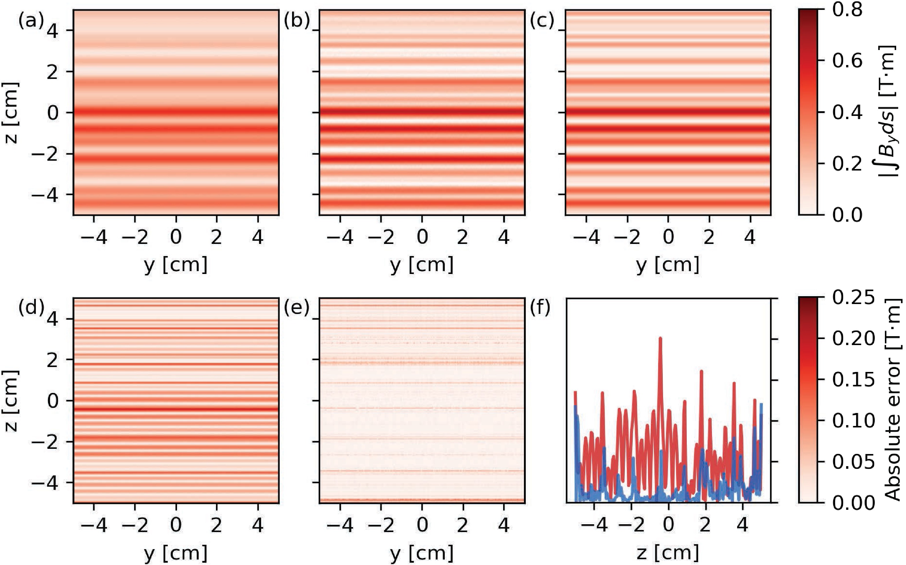
Figure 8. (color online) (a) Reconstructed path-integrated magnetic field strength without spectral amplitude compensation. (b) Reconstructed path-integrated magnetic field strength with spectral amplitude compensation. (c) Path-integrated magnetic field calculated from analytical formula. (d) Absolute error of reconstruction without spectral amplitude compensation. (e) Absolute error of reconstruction with spectral amplitude compensation. (f) Absolute errors along the y-axis. The blue and red solid lines correspond to cases with and without spectral amplitude compensation, respectively.
$ \begin{aligned} B_y = \sum_{i=1}^{10} B_i\exp\left(-(x-x_0)^2/w_x^2\right)\cos\left(2\pi z/{\lambda_z}_i+\psi_i\right). \end{aligned} $

(17) The wavelengths of each mode
$ {\lambda_z}_i $ are randomly selected from 100 to 700$ \mu\text{m} $ , and the field strengths$ B_i $ are randomized between 1000 and 2000 T. The path-integrated magnetic field strength calculated from the analytical formula (17), as shown in Fig. 8(c), is used as the reference to quantitively estimate the reconstruction errors. The absolute errors of the path-integrated magnetic field strength reconstructions without and with compensation are shown in Fig. 8(d) and 8(e), respectively. The absolute errors along the y-axis are shown in Fig. 8(f). Without compensation, the reconstructed path-integrated magnetic field strength exhibits large discrepancies with the reference. The application of compensation results in a notable reduction in absolute errors across the majority of areas, with the exception of those situated in proximity to boundaries. This is because the periodic boundary condition of the Fourier transform is not a valid assumption in such cases.Neutrons can be deflected by the Stern-Gerlach force in non-uniform magnetic fields,
$ \begin{aligned} {\boldsymbol{F}}_{SG} = \nabla {\boldsymbol{\mu}}\cdot{\boldsymbol{B}}=\gamma_n\nabla\left(s_xB_x+s_yB_y+s_zB_z\right), \end{aligned} $

(18) where
$ {\boldsymbol{\mu}} $ is the magnetic moment, and$ s_x,s_y,s_z=\pm\hbar/2 $ are spin eigenvalues. The trajectories of neutrons passing through a magnetic field given by Eq. (13) are numerically calculated and shown in Fig. 9. The magnetic field has only a y-component. Neutrons with different eigenvalues$ s_y $ are split by the magnetic field gradient in the z-direction. For neutrons with energies of 10 eV and 100 eV, the deflection angles are much larger than those of the 14.1 MeV neutrons. For the 14.1 MeV neutrons, the distance between neutrons with different eigenvalues on the detector at 1 m is only 58 pm. Thus, the effects of Stern-Gerlach force are negligible for the 14.1 MeV neutrons.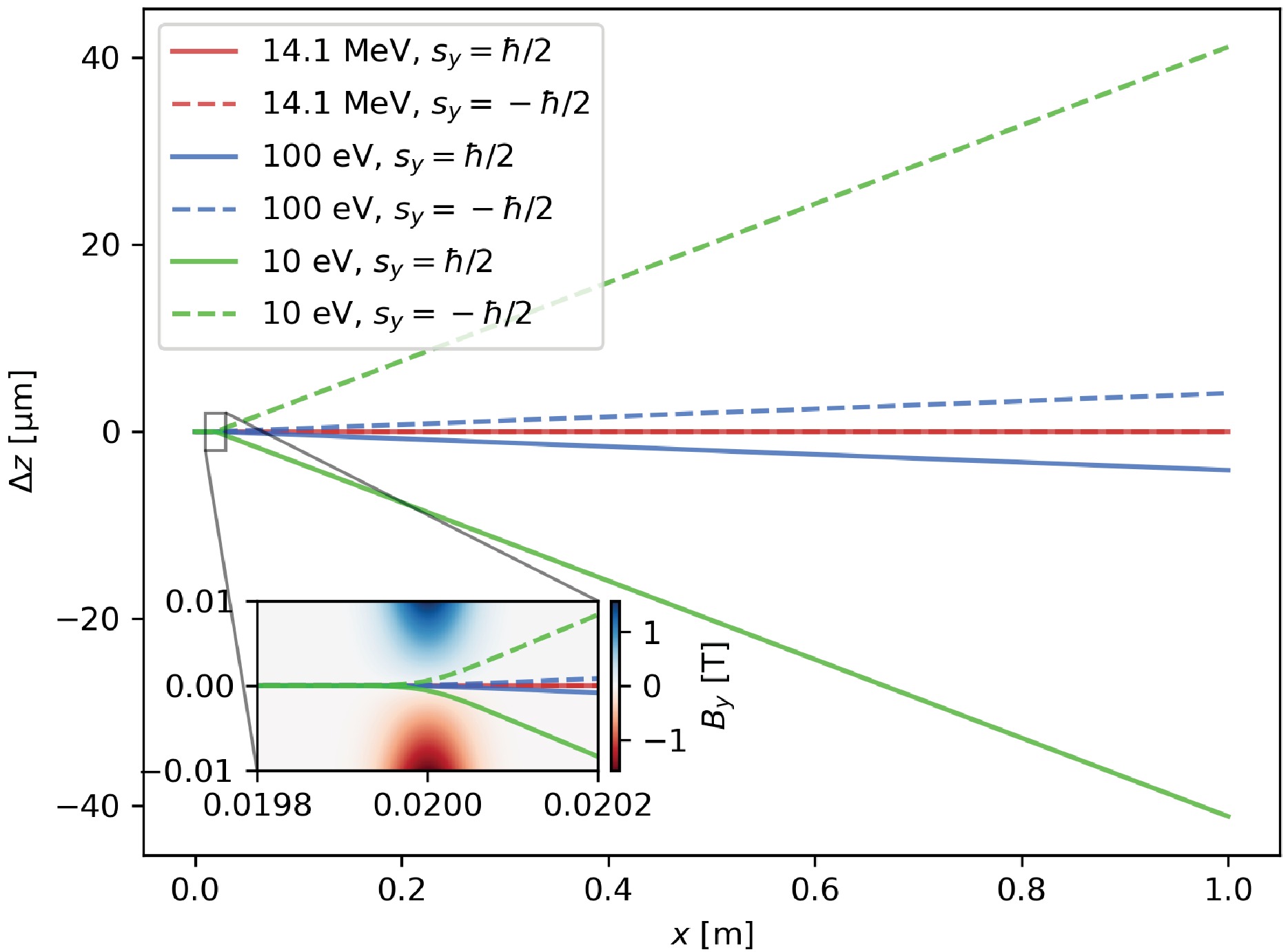
Figure 9. (color online) Trajectories of neutrons with different energies and spin eigenvalues passing through the magnetic field with
$ \lambda_z=200 $ $ \mu\text{m} $ . -
Monte Carlo simulations are used to investigate the polarized neutron imaging of magnetic fields with the polarized neutron source from the imploded capsule. The macro-particle representing neutrons is initialized with random positions according to the emissivity distribution shown in Fig. 3(a). The energies of the neutrons are 14.1 MeV, and the velocity directions are sampled from the angular distribution given by the SPINSIM simulation. As mentioned in Sec. III, the spatial and angular distributions of the neutron source are stored in six 3D arrays. As only the static magnetic field imaging is investigated in this study, the temporal effects are not considered. To investigate temporal effects, 4D arrays should be used to include the temporal variations of the neutron source. The coordinates of a computational cell
$ (i,j,k) $ are$ (x_{i,j,k}, \ y_{i,j,k},\ z_{i,j,k}) $ , and the neutron yield in the cell is$ N_{i,j,k} $ . The differential yields in each cell are$ \begin{aligned}[b] \frac{{\rm d}}{N_{i,j,k}}{{\rm d}\Omega}=\; &\frac{{\rm d}N_{i,j,k}^+}{{\rm d}\Omega}+\frac{{\rm d}N_{i,j,k}^-}{{\rm d}\Omega}\\ =\; &{C_1}_{i,j,k}\sin^2\theta+{C_2}_{i,j,k}\left(3\cos^2\theta+1\right),\\ \frac{{\rm d}N_{i,j,k}^+}{{\rm d}\Omega}-\frac{{\rm d}N_{i,j,k}^-}{{\rm d}\Omega}=\; &{C_3}_{i,j,k}\sin^2\theta \cos^2\theta\\ & +{C_4}_{i,j,k}\sin^4\theta+{C_5}_{i,j,k}\left(3\cos^2\theta-1\right)^2, \end{aligned} $
(6) where
$ \dfrac{{\rm d}N}{{\rm d}\Omega} $ is the total differential yield,$ \dfrac{{\rm d}N^\pm}{{\rm d}\Omega} $ are the differential yields for$ m_z=\pm\dfrac{1}{2} $ states, respectively, and$ C_1 $ -$ C_5 $ are the coefficients calculated from Eqs. (4) and (5). The random spatial and velocity distributions of macro-particles are generated from the six 3D arrays N and$ C_1 $ -$ C_5 $ with the inverse cumulative distribution function (CDF) method. The 3D arrays are flattened into 1D arrays by introducing a new index$ l=iN_yN_z+jN_z+k $ , where$ N_x $ ,$ N_y $ ,$ N_z $ are the numbers of grid cells in x, y, and z directions, respectively. The discretized CDF of the spatial distribution can be calculated as$ \begin{aligned} F_l = \sum_0^l N_l/\sum_0^{N_xN_yN_z} N_l. \end{aligned} $
(7) For each particle, a random number
$ p_0 $ is generated from the uniform distribution$ [0,1) $ , and the cell index of the particle is determined by$ F_{l-1}\leq p_0 <F_l $ . The particle coordinate can be calculated as$ \begin{aligned} x = x_l + p_1 {\rm d}x,\ y = y_l + p_2 {\rm d}y,\ z = z_l + p_3 {\rm d}z, \end{aligned} $
(8) where
$ p_1 $ -$ p_3 $ are random numbers from the uniform distribution$ [0,1) $ .$ {\rm d}x $ ,$ {\rm d}y $ , and$ {\rm d}z $ are the cell sizes. The CDF of the angular distribution is$ \begin{aligned}[b] G_l(\theta)=\;&\frac{\int_0^{\pi/2-\theta_m}\left({C_1}_l\sin^2\theta+{C_2}_l\left(3\cos^2\theta+1\right)\right)\sin\theta {\rm d}\theta}{\int_{\pi/2-\theta_m}^{\pi/2+\theta_m}\left({C_1}_l\sin^2\theta+{C_2}_l\left(3\cos^2\theta+1\right)\right)\sin\theta {\rm d}\theta}\\ &\begin{aligned}=[(&{C_2}_l-{C_1}_l/3)(\sin^3\theta_m-\cos^3\theta)+\\ (&{C_2}_l+{C_1}_l)(\sin\theta_m-\cos\theta)]/\\ [(&{C_2}_l-{C_1}_l/3)(2\sin^3\theta_m)+({C_2}_l+{C_1}_l)(2\sin\theta_m)].\end{aligned} \end{aligned} $
(9) Neutrons with divergence angles larger than
$ \theta_m= \arctan((L_z/2+z_{\rm max})/(x_s-x_{\rm max})) $ are located outside the detector, so they are neglected in the simulation to reduce computational cost.$ L_z $ is the detector length in the z direction, while$ x_s $ is the x coordinate of the detector, and$ x_{\rm max} $ and$ z_{\rm max} $ are the largest neutron coordinates in the x and z directions, respectively. By solving the equation$ G_l(\theta)=p_4 $ , one can obtain the polar angle θ for the macro-particle, where$ p_4 $ is from the uniform distribution$ [0,1) $ . The azimuthal angle is obtained by$ \phi=(2p_5-1)\phi_m $ , where$ p_5 $ is also from the uniform distribution$ [0,1) $ ,$ \phi_m= \arctan((L_y/2+y_{\rm max})/(x_s-x_{\rm max})) $ .$ (\theta,\phi) $ determines the velocity direction of the macro-particle. The macro-particle used in the simulation represents a statistical ensemble of numerous real particles. The number of such particles determines the weight of the macro-particle. The weight of a macro-particle is calculated as$ \begin{aligned} w=\frac{4\phi_m}{N_p}\left[({C_2}_l-{C_1}_l/3)\sin^3\theta_m+({C_2}_l+{C_1}_l)\sin\theta_m\right], \end{aligned} $
(10) where
$ N_p $ is the total number of macro-particles. The neutron spin states can be described by the spin vector. The spin states of the macro-particle are described by the ensemble average of spin vectors$ \left<{\boldsymbol{s}}\right>=(\left<s_x\right>, \left<s_y\right>, \left<s_z\right>) $ . The azimuthal angles of spin vectors are random, so$ \left<s_x\right> $ and$ \left<s_y\right> $ are both zero.$ \left<s_z\right> $ is calculated as$ \begin{aligned} \left<s_z\right>=\frac{{C_3}_l\sin^2\theta \cos^2\theta+{C_4}_l\sin^4\theta+{C_5}_l\left(3\cos^2\theta-1\right)^2}{{C_1}_l\sin^2\theta+{C_2}_l\left(3\cos^2\theta+1\right)}. \end{aligned} $
(11) The spin precession of the macro-particle in magnetic fields can be described by [25]
$ \begin{aligned} \frac{{\rm d}\left<{\boldsymbol{s}}\right>}{{\rm d}t}=\gamma_n\left<{\boldsymbol{s}}\right>\times{\boldsymbol{B}}, \end{aligned} $
(12) where
$ \gamma_n $ =$ -1.83\times10^8 $ $ \text{rad}/(\text{s}\cdot \text{T}) $ is the gyromagnetic ratio of a neutron, and$ {\boldsymbol{B}} $ is the magnetic field vector. For constant magnetic fields, Eq. (12) can be solved analytically. The spin vector rotates around the magnetic field with a constant frequency$ \omega_L=\gamma_n|B| $ , known as the Larmor frequency. To solve Eq. (12) for a time-varying magnetic field, the discrete time step$ {\rm d}t $ should be sufficiently small, and the magnetic field is assumed to be constant within each time step. At each time step, the analytical solution is used to advance the spin precession. For a magnetic field rotating around the x-axis with a frequency of$ \omega_B $ and constant strength of 1 T, the numerical solutions obtained for different time step sizes are compared with the analytical solution in adiabatic approximation, as shown in Fig. 5. The adiabatic approximation assumes that the spin vector locally precesses around the instant direction of the magnetic field, which is valid when$ \omega_B\ll \omega_L $ . For$ \omega_B=0.1\omega_L $ , our numerical solutions agree well with the adiabatic solution, as shown in Fig. 5(a). For$ \omega_B=0.7\omega_L $ , the adiabatic approximation is no longer valid, as evidenced by the discrepancy between the adiabatic solution and our numerical solution, as illustrated in Fig. 5(b). Because we use the analytical solution to advance the spin precession, the time step$ {\rm d}t $ does not need to be significantly smaller than the Larmor period$ T_L=2\pi/\omega_L $ , as in the finite difference method. The time step$ {\rm d}t $ only needs to be much smaller than the characteristic time scale of the varying magnetic field; in this case, the period of rotation$ T_B=2\pi/\omega_B $ . For$ {\rm d}t=T_B/40 $ , our numerical solution can already give consistent results with a highly resolved solution, as shown in Figs. 5(a) and 5(b).
Figure 5. (color online) Comparison of the analytical solution in adiabatic approximation and numerical solutions with different time step sizes
$ {\rm d}t $ of the spin precession Eq. (12). The z component of the spin vector$ \left<s\right> $ is shown. The magnetic field rotates around the x-axis with (a)$ \omega_B=0.1\omega_L $ , (b)$ \omega_B=0.7\omega_L $ , where$ \omega_B $ is the angular frequency of the rotating magnetic field,$ \omega_L $ is the Larmor frequency, and$ T_B=2\pi/\omega_B $ is the rotation period of the magnetic field.The magnetic field used in the Monte Carlo simulation is given by
$ \begin{aligned} B_y = B_0\exp\left(-(x-x_0)^2/w_x^2\right)\cos\left(2\pi z/\lambda_z+\psi\right). \end{aligned} $
(13) The magnetic field has only a y component. The neutron beam propagates along the
$ +x $ direction (longitudinal direction), and the neutron polarization is along the z direction.$ B_0 $ is the peak magnetic field strength. In addition,$ x_0 $ is the longitudinal center of the magnetic field, and$ w_x $ is the longitudinal width of the magnetic field. In the simulation, magnetic field strength and longitudinal width are chosen close to the laser-driven HED conditions, with$ B_0=5000 $ T and$ w_x=50\ \mu\text{m} $ . The magnetic field is periodic along the z direction with a wavelength of$ \lambda_z $ and phase of ψ. The neutron source is placed at the origin. The magnetic field center is at$ x_0=2 $ cm, and three neutron detectors are placed at 1 m from the source. Macro-particles move from their initial positions to the detectors in straight lines. The evolution of the spin vector in magnetic field is calculated for each macro-particle. The time step size used to solve spin precession (Eq. (12)) is$ {\rm d}t=w_x/(51.2v_n) $ , where$ v_n $ is the neutron velocity. The counts of the macro-particles are added to the detectors, which have dimensions of 10×10 cm and a pixel resolution of 200×200. The neutron source is a point-like source with small source sizes, and the geometric magnification of the detector image is 50. The first neutron detector measures the neutron fluence$ F_1(y,z) $ of the spin down state after passing through the magnetic field. The second neutron detector measures the neutron fluence$ F_2(y,z) $ of the spin down state without passing through the magnetic field. The third neutron detector measures the neutron fluence$ F_3(y,z) $ of both the spin up and down states. The initial neutron polarization can be calculated as$ P_{z0}^n(y,z)=1-2F_2/F_3 $ , and the neutron polarization after passing through the magnetic field is$ P_z^n(y,z)= 1-2F_1/F_3 $ . For an ideal point source, the path-integrated magnetic field strength can be given by$ \begin{aligned} \left|\int B_y {\rm d}s\right| = \frac{v_n}{\gamma_n}\left(\pi-\arccos(P_z^n/\left|P_{z0}^n\right|)\right). \end{aligned} $
(14) For a finite-size source, neutrons from different source positions experience different magnetic fields and then meet at the detector. To obtain the path-integrated magnetic field strength using finite-size sources, a deblurring algorithm is proposed, which is discussed in the following section.
The polarizations of neutrons from different sources after passing through the magnetic field are depicted in Fig. 6. Figure 6(a) shows the results of neutrons from an ideal point source, with an initial neutron polarization of
$ -1 $ , passing through magnetic fields with a wavelength$ \lambda_z=200\ \mu\text{m} $ . The neutron polarization distributions are modulated by the periodic magnetic field. The modulation wavelength of the detector image is 0.5 cm, corresponding to a magnetic field strength variation wavelength of 100$ \mu\text{m} $ due to a geometric magnification of 50. As shown in Eq. (14), the polarized neutron imaging can only measure the absolute strength of the magnetic field. The variation wavelength of the magnetic field strength$ |B| $ is$ \lambda_z/2 $ . The neutron polarization image of a Gaussian source with an FWHM of 80$ \mu\text{m} $ and initial neutron polarization of$ -1 $ is shown in Fig. 6(b). The amplitude of the polarization modulation in this case is smaller than that in the point source case due to the finite-size-source blurring effect. The amplitude of the polarization modulation for the imploded-capsule source is also smaller than that of the point source case, as shown in Fig. 6(c). For the ideal point source, the spatial resolution is limited only by the resolution and signal-to-noise ratio of the detector. With sufficiently high detector resolution and signal-to-noise ratio, the 50$ \mu\text{m} $ wavelength corresponding to the magnetic field strength variation can be resolved by the ideal point source, as illustrated in Fig. 6(d). However, for the Gaussian source and the imploded-capsule source, both with an FWHM of 80$ \mu\text{m} $ , the 50$ \mu\text{m} $ variation wavelength can barely be resolved even when the detector resolution and signal-to-noise ratio are sufficiently high, as shown in Figs. 6(e) and 6(f).
Figure 6. (color online) Neutron polarization distributions after passing through the magnetic field. (a) Point source and magnetic field strength variation wavelength of 100
$ \mu\text{m} $ . (b) Gaussian source with FWHM of 80$ \mu\text{m} $ and magnetic field strength variation wavelength of 100$ \mu\text{m} $ . (c) Imploded-capsule source with FWHM of 80$ \mu\text{m} $ and magnetic field strength variation wavelength of 100$ \mu\text{m} $ . (d) Point source and magnetic field strength variation wavelength of 50$ \mu\text{m} $ . (e) Gaussian source with FWHM of 80$ \mu\text{m} $ and magnetic field strength variation wavelength of 50$ \mu\text{m} $ . (f) Imploded-capsule source with FWHM of 80$ \mu\text{m} $ and magnetic field strength variation wavelength of 50$ \mu\text{m} $ .Using the neutron polarizations of the finite-size source in Eq. (14) will lead to an incorrect path-integrated magnetic field strength. The decrements in the neutron polarization modulations of the finite-size sources are quantitively calculated and shown in Fig. 7. The discrete Fourier transforms (DFTs) of the neutron polarization distributions along the y-axis are shown in Fig. 7(a). The wavelength corresponding to the magnetic field strength variation is
$ 100\ \mu\text{m} $ , and the first-order peaks of the spectra are located at 0.01$ \mu\text{m}^{-1} $ . In the point source case, the spectrum has multiple peaks, indicating high-order components. For the imploded-capsule source, due to the finite-source-size blurring, the amplitude of the first-order peak is smaller than that of the point source case, and the high-order components are missing. The spectral loss rate is defined as the ratio of amplitudes of the first-order peaks of the finite-size source and point source. The spectral loss rates of different sources as functions of the magnetic field strength variation wavelength are shown in Fig. 7(b). The spectral loss rate increases with the characteristic wavelength and decreases with the source size. An empirical formula for the spectral loss rate is obtained by fitting the simulation results, which can be written as
Figure 7. (color online) (a) DFT spectra of the neutron polarization distributions along the y-axis for the point source and imploded-capsule source. (b) Spectral loss rates as functions of the characteristic wavelengths for Gaussian sources with different source sizes and the imploded-capsule source. The circles denote the Monte Carlo simulation results, and solid lines are curves fitted using Eq. (15).
$ \begin{aligned} L(\lambda)=\frac{1}{\left[1+\left(s/2\lambda\right)^2\right]^{14}}, \end{aligned} $
(15) where
$ L(\lambda) $ is the spectral loss rate, λ is the characteristic wavelength, and s is the fitting parameter. The results of the fitting are illustrated as solid curves in Fig. 7(b). For Gaussian sources, it is found that s is equal to the FWHM of the source. For the imploded-capsule source with an FWHM of 80$ \mu\text{m} $ , s is equal to 65$ \mu\text{m} $ .By employing the spectral loss rate, the decrement in the amplitude of neutron polarization variation can be compensated. The compensated neutron polarization distribution can be written as
$ \begin{aligned} P_z^{n*}=\text{Re}\left\{{\cal{F}}^{-1}_y\left\{{\cal{F}}_y\left\{P_z^n\right\}/L(\lambda)\right\}\right\}, \end{aligned} $
(16) where
$ {\cal{F}}_y $ is the Fourier transform in the y direction, and$ {\cal{F}}_y^{-1} $ is the inverse Fourier transform. Equation (16) is the general expression used for the spectral amplitude compensation. In practice,$ L(\lambda) $ is manually set to 1 for$ \lambda<s $ to avoid the amplification of high-frequency noise. The values of$ P_z^{n*} $ that are larger than 1 or smaller than -1 are manually set to 1 and -1, respectively. Substituting the neutron polarization distribution,$ P_z^n $ , in Eq. (14) with the compensated neutron polarization distribution,$ P_z^{n*} $ , the resulting path-integrated magnetic field strength is more accurate. The reconstructed path-integrated magnetic field strengths using$ P_z^n $ and$ P_z^{n*} $ are shown in Figs. 8(a) and 8(b), respectively. The magnetic field is a sum of ten modes with random field strengths, wavelengths, and phases, and it is expressed as
Figure 8. (color online) (a) Reconstructed path-integrated magnetic field strength without spectral amplitude compensation. (b) Reconstructed path-integrated magnetic field strength with spectral amplitude compensation. (c) Path-integrated magnetic field calculated from analytical formula. (d) Absolute error of reconstruction without spectral amplitude compensation. (e) Absolute error of reconstruction with spectral amplitude compensation. (f) Absolute errors along the y-axis. The blue and red solid lines correspond to cases with and without spectral amplitude compensation, respectively.
$ \begin{aligned} B_y = \sum_{i=1}^{10} B_i\exp\left(-(x-x_0)^2/w_x^2\right)\cos\left(2\pi z/{\lambda_z}_i+\psi_i\right). \end{aligned} $
(17) The wavelengths of each mode
$ {\lambda_z}_i $ are randomly selected from 100 to 700$ \mu\text{m} $ , and the field strengths$ B_i $ are randomized between 1000 and 2000 T. The path-integrated magnetic field strength calculated from the analytical formula (17), as shown in Fig. 8(c), is used as the reference to quantitively estimate the reconstruction errors. The absolute errors of the path-integrated magnetic field strength reconstructions without and with compensation are shown in Fig. 8(d) and 8(e), respectively. The absolute errors along the y-axis are shown in Fig. 8(f). Without compensation, the reconstructed path-integrated magnetic field strength exhibits large discrepancies with the reference. The application of compensation results in a notable reduction in absolute errors across the majority of areas, with the exception of those situated in proximity to boundaries. This is because the periodic boundary condition of the Fourier transform is not a valid assumption in such cases.Neutrons can be deflected by the Stern-Gerlach force in non-uniform magnetic fields,
$ \begin{aligned} {\boldsymbol{F}}_{SG} = \nabla {\boldsymbol{\mu}}\cdot{\boldsymbol{B}}=\gamma_n\nabla\left(s_xB_x+s_yB_y+s_zB_z\right), \end{aligned} $
(18) where
$ {\boldsymbol{\mu}} $ is the magnetic moment, and$ s_x,s_y,s_z=\pm\hbar/2 $ are spin eigenvalues. The trajectories of neutrons passing through a magnetic field given by Eq. (13) are numerically calculated and shown in Fig. 9. The magnetic field has only a y-component. Neutrons with different eigenvalues$ s_y $ are split by the magnetic field gradient in the z-direction. For neutrons with energies of 10 eV and 100 eV, the deflection angles are much larger than those of the 14.1 MeV neutrons. For the 14.1 MeV neutrons, the distance between neutrons with different eigenvalues on the detector at 1 m is only 58 pm. Thus, the effects of Stern-Gerlach force are negligible for the 14.1 MeV neutrons.
Figure 9. (color online) Trajectories of neutrons with different energies and spin eigenvalues passing through the magnetic field with
$ \lambda_z=200 $ $ \mu\text{m} $ . -
The polarized neutron beams from polarized DT gas-filled capsule implosion are characterized with 3D STHD simulations. The FWHM source size of the neutron source can be lower than 100
$ \mu\text{m} $ . With sufficiently high detector resolution and signal-to-noise ratio, the spatial resolution of the polarized neutron imaging can reach sub-100$ \mu\text{m} $ . The synthetic polarized neutron images are obtained with Monte Carlo simulations. For finite-size sources, the finite-source-size blurring effect reduces the amplitudes of neutron polarization perturbations. The spectral loss rate function can be used to compensate the decrement in neutron polarization perturbation and reduce the error in magnetic field reconstruction. The spectral loss rate function is a unique property of the neutron source, which is determined by the spatial and angular distributions of the neutron source. The spatial and angular distributions of the neutron sources are routinely measured in ICF experiments [39]. The measured spatial and angular distributions can then be used as the input for Monte Carlo simulations to obtain the spectral loss rate function for the neutron source.The polarized neutron beam from polarized DT fusion is a novel and unique tool to probe the magnetic fields in HED plasmas. Compared to the well-developed proton imaging technique, which reconstructs the magnetic field from the degree of proton deflection, polarized neutron imaging utilizes the degree of neutron spin precession to record the magnetic field strength. Polarized neutron imaging has more degrees of freedom, and the magnetic field reconstruction is more straightforward because the neutrons are not deflected by the magnetic fields. In contrast to cold and thermal neutrons, the 14 MeV fast neutrons have higher penetration depths in many materials [40], allowing them to probe magnetic fields inside dense HED plasmas. The magnetic fields present in laser-generated HED plasmas are transient and exhibit shot-to-shot variations. Single-shot imaging is required to capture the shot-to-shot differences in the magnetic fields, which demands a polarized neutron source with a high flux and short pulse duration. The donut-shaped polarized neutron beams from the imploded DT target with parallel polarization allow single-shot measurements of neutrons in different polarization states with and without magnetic fields, which are necessary for the magnet field reconstruction. Conventional spin filters, such as the polarized helium-3 filter, are designed for cold and thermal neutrons. The functionality and efficiency of spin filters for fast neutrons must be further investigated.
-
The polarized neutron beams from polarized DT gas-filled capsule implosion are characterized with 3D STHD simulations. The FWHM source size of the neutron source can be lower than 100
$ \mu\text{m} $ . With sufficiently high detector resolution and signal-to-noise ratio, the spatial resolution of the polarized neutron imaging can reach sub-100$ \mu\text{m} $ . The synthetic polarized neutron images are obtained with Monte Carlo simulations. For finite-size sources, the finite-source-size blurring effect reduces the amplitudes of neutron polarization perturbations. The spectral loss rate function can be used to compensate the decrement in neutron polarization perturbation and reduce the error in magnetic field reconstruction. The spectral loss rate function is a unique property of the neutron source, which is determined by the spatial and angular distributions of the neutron source. The spatial and angular distributions of the neutron sources are routinely measured in ICF experiments [39]. The measured spatial and angular distributions can then be used as the input for Monte Carlo simulations to obtain the spectral loss rate function for the neutron source.The polarized neutron beam from polarized DT fusion is a novel and unique tool to probe the magnetic fields in HED plasmas. Compared to the well-developed proton imaging technique, which reconstructs the magnetic field from the degree of proton deflection, polarized neutron imaging utilizes the degree of neutron spin precession to record the magnetic field strength. Polarized neutron imaging has more degrees of freedom, and the magnetic field reconstruction is more straightforward because the neutrons are not deflected by the magnetic fields. In contrast to cold and thermal neutrons, the 14 MeV fast neutrons have higher penetration depths in many materials [40], allowing them to probe magnetic fields inside dense HED plasmas. The magnetic fields present in laser-generated HED plasmas are transient and exhibit shot-to-shot variations. Single-shot imaging is required to capture the shot-to-shot differences in the magnetic fields, which demands a polarized neutron source with a high flux and short pulse duration. The donut-shaped polarized neutron beams from the imploded DT target with parallel polarization allow single-shot measurements of neutrons in different polarization states with and without magnetic fields, which are necessary for the magnet field reconstruction. Conventional spin filters, such as the polarized helium-3 filter, are designed for cold and thermal neutrons. The functionality and efficiency of spin filters for fast neutrons must be further investigated.
Polarized neutron beams from polarized deuterium-tritium fusion with applications to magnetic field imaging in high-energy-density plasmas
- Received Date: 2025-03-25
- Available Online: 2025-12-15
Abstract: When the spins of deuteron and triton are aligned in parallel, the fusion cross-section increases by approximately 50%. The emitted neutrons are anisotropic and polarized in specific directions. The polarized neutron beams can be used to measure strong magnetic fields in high-energy-density plasmas, offering a potential alternative to the well-established proton imaging technique. In contrast to protons, neutrons are not deflected by electromagnetic fields and are not sensitive to electric fields, thus reducing the complexity of magnetic field reconstruction. Three-dimensional spin transport hydrodynamics simulations are employed to investigate the polarized neutron beams generated from spin-polarized deuterium-tritium target implosions. Synthetic polarized neutron images of magnetic fields are generated from Monte Carlo simulations. Based on a comparison of the results of finite-size sources and an ideal point source, a method to compensate the finite-source-size blurring effect is proposed to reduce the error in magnetic field reconstruction.


 DownLoad: