Extraction of nuclear imaginary potential from the excitation function of backward quasi-elastic scattering

The nucleus-nucleus interaction potential is a fundamental physical quantity in the study of heavy-ion nuclear reactions, mainly consisting of the repulsive Coulomb potential and absorptive nuclear potential: $ U(r)=V_C(r)+V_N(r) $ [1]. The nuclear potential is a crucial component, serving as a construct to account for the many-body interactions between the protons and neutrons in the two interacting nuclei that are not explicitly included through channel couplings. Unlike the good calculation for the Coulomb potential, the nuclear potential is not well described till now.

The commonly used nuclear potential is the optical model potential (OMP), written as $ V_N(r)=V(r)+{\rm{i}} W(r) $, consists of an attractive real part and an absorptive imaginary part [2]. The real part and imaginary part optical potential parameters have been generally extracted from the analysis of elastic scattering data [3, 4]. Because of the strong absorption in heavy-ion reactions, the angular distributions for elastic scattering are most sensitive to the tail region of the potential. Therefore, the optical potential extracted from fitting the elastic scattering angular distribution is not unique, exhibiting Igo ambiguity [5]. In order to avoid Igo ambiguity of the optical potential parameters, the real part optical potential can be well calculated using microscopic methods, such as the folding model potential [6] or the proximity potential [7, 8], but the imaginary part, such as obtained by complex G-matrix [9], is often difficult to be satisfied. Therefore, the imaginary part of the phenomenological optical potential is generally used instead.

The optical potential can also be extracted from other reaction channels, such as transfer [10, 11], fusion [12, 13, 14] and quasi-elastic scattering [15]. Extracting the optical potential parameters using the transfer channel can make up for the shortcomings of the elastic scattering method that is not sensitive to the low energy region, but for the systems with obvious coupling effects, the shortcoming is calling for complex coupled reaction channels (CRC) calculation [10]. For systems with obvious coupling effects, under the incoming wave boundary condition (IWBC) approximation [16], the real part of the optical potential can be extracted from the fusion data using barrier tunneling [12], but the imaginary part of the nuclear potential is not introduced in this approximation. It is essential to recognize that the analysis and conclusions through fusion reaction could only be achieved following the measurement of precise experimental fusion data [17], which is experimentally difficult.

Backward quasi-elastic scattering (QEL) has been shown to be a valuable way to study the nuclear potential, particularly since backward quasi-elastic scattering experimental data are easier and more efficient to be measured compared to fusion experiments [18]. QEL is defined as the sum of elastic scattering, inelastic scattering, and nucleon transfer process. Thus, backward quasi-elastic scattering and fusion are complementary to each other. In general, a short-range imaginary potential with $ W = 30 $ MeV, $ r_{0W} = 1.0 $ fm, and $ a_W = 0.4 $ fm was used to simulate the compound nucleus formation [19]. It was mentioned [20] that the calculated results were insensitive to the parameters of the imaginary part of the potential as long as it is strong enough and well localized inside the Coulomb barrier. However, this choice for the parameters of imaginary part potential is somewhat arbitrary and can not fit the data in the higher energy region. The fit to the experimental data was not improved even if varying the depth, the radius and the diffuseness parameters of the real part potential as well as the deformation parameters [20]. The discrepancy between the experimental data and the theoretical calculation for the quasi-elastic excitation function is due to the effect of nuclear distortion with decreasing distance for the two reactants.

To understand nuclear interaction potentials in the energy region around the Coulomb barrier for the systems $ ^{16} $O with heavy and well-deformed nuclei $ ^{152,154} $Sm and $ ^{184,186} $W, we propose a novel method that to extract the nuclear potential from the high-precision excitation function of backward quasi-elastic scattering. In the previous works, the real part potentials are well described, the parameters may be constrained by requiring that the calculations are consistent with fusion measurements and quasielastic scattering [21, 22]. They may also be taken from systematic parameterizations [7] of fits to elastic scattering data. However, the description of imaginary potential is insufficient. Therefore, we tried to extract the imaginary part potential from backward quasi-elastic excitation function in the case of fixed real part potential in this work. The bare potential can be extracted in coupled-channels (CC) calculation, and the effective potential can be extracted in single-channel (SC) calculation. It should be noted that the bare potential extracted here by using CC calculation is an empirical bare potential. In practice, it is not possible to include all conceivable couplings in CC calculations. For the well-deformed nuclei, the coupling of deformation is explicitly emphasized in CC calculation. Transfer channels might also play an important role in backward quasi-elastic scattering [23]. Unfortunately, including transfer channels in CC calculations is quite challenging. Therefore, in this paper, we try to incorporate the strong absorption effect within the imaginary potential by adjusting the parameters of the imaginary potential.

The organization of this paper is as follows. We briefly explain the coupled-channels formalism for backward quasi-elastic scattering in Section 2. The results of CC and SC calculations are given in Section 3. We summarize the paper in Section 4.

This section provides a brief description of coupled-channels approach (CCFULL [24]) used in the present study. The coupled-channel model CCFULL has been detailed described in [19, 25].

The total Hamiltonian used in the coupled-channels formalism by taking into account the intrinsic excitations of the colliding nuclei is given

where $ \bf{r} $ represents the coordinate for the relative motion between the target and the projectile nuclei, μ is the reduced mass and $ \xi_T $ and $ \xi_P $ are the coordinate of the intrinsic motion in the target and the projectile nuclei, respectively. $ V^{(0)}_ N $ is the bare nuclear potential. It is assumed to have a Woods-Saxon shape and consists of the real and imaginary parts,

where $ V_0 $, $ R_0 $, and a are the depth, radius, and the diffuseness parameters of real part potential; W, $ R_W $, and $ a_W $ are the depth, radius, and the diffuseness parameters of imaginary part potential, respectively. $ V_C(r) $ is the Coulomb potential, given by [26],

where $ Z_P $ and $ Z_T $ are the projectile and target charge number, Coulomb radius $ R_C=r_C(A^{1/3}_T + A^{1/3}_P) $ with $ A_T $ and $ A_P $ are the mass number of the target and projectile nuclei, respectively. $ H_{\rm{exct}} $ describes the excitation spectra of the target and projectile nuclei, whereas $ V_{\rm{coup}}({\bf{r}},\xi_P,\xi_T) $ is the potential for the coupling between the relative motion and the intrinsic excitations of the target and projectile nuclei.

In the iso-centrifugal approximation [24, 27, 28], where the angular momentum of the relative motion in each channel is replaced with the total angular momentum J, the coupled-channels equations derived from the Hamiltonian (1) is obtained to be

where $ \epsilon_n $ is the eigenenergy for the nth channel. $ V_{nm}(r) $ are the matrix elements for the coupling potential $ V_{\rm{coup}} $.

The intrinsic coordinates $ \xi_P $ and $ \xi_T $ in the coupling potential, $ V_{\rm{coup}} $, is replaced with the dynamical operators $ {\hat{O}}_P $ and $ {\hat{O}}_T $. In this way, the coupling potential is given by

In order to avoid double counting, we have subtracted $ V^{(0)}_N(r) $ in Equation (6).

For deformed target nucleus,

is used for rotational coupling, where the target radius $ R_T = r_T A_T^{1/3} $, $ Y_{\lambda 0} $ is the spherical harmonics and $ \beta_2 $, $ \beta_4 $ are the quadrupole and hexadecapole deformation parameters of the target nucleus, respectively. These deformation parameters quantify the deviation from spherical symmetry and are critical for describing rotational excitations in well-deformed nuclei. The coupling matrix element between the $ \left| {{n}} \right\rangle=\left| {{I0}} \right\rangle $ and $ \left| {{m}} \right\rangle=\left| {{I'0}} \right\rangle $ states of the ground rotational band of the target is given by [25]

and $ \hat{O} $ satisfies

The nuclear coupling matrix elements are then evaluated as

The last term in this equation is included to avoid the double counting of the diagonal component.

For the Coulomb interaction of the deformed target, the matrix elements are then given by

where

The total coupling matrix element is given by the sum of $ V_{nm}^{(N)} $ and $ V_{nm}^{(C)} $.

The coupled-channels equations, Equation (1), are solved with the scattering boundary condition for $ u_n(r) $ [19]

where $ S_n^J $ is the nuclear S-matrix. $ H_J^{(-)}(k_n r) $ and $ H_J^{(+)}(k_n r) $ are the incoming and the outgoing Coulomb wave functions, respectively. The channel wave number $ k_n $ is given by $ \sqrt{2\mu(E-\epsilon_n)/{\hbar^2}} $ and $ k_i = \sqrt{2\mu E/ {\hbar^2}} $. The scattering angular distribution for the channel n is then given by

with

here $ \sigma_J(E) $ and $ f_C(\theta) $ are the the Coulomb phase shift and the Coulomb scattering amplitude, respectively. The differential quasi-elastic cross section is then calculated to be

One will apply this formalism to perform the coupled-channels analysis for the backward quasi-elastic scattering of all systems.

In this section, we present the results of our detailed coupled-channels analysis for large angle quasi-elastic scattering data of $ ^{16} $O$ +^{152,154} $Sm, $ ^{184,186} $W systems. The experiment was performed at the HI-13 tandem accelerator of the China Institute of Atomic Energy. More details can be found in [15].

Differential cross section for quasi-elastic events at each beam energy was normalized with Rutherford scattering cross section. The center-of-mass enerey ($ E_{\text{c.m.}} $) was corrected for centrifugal effects at each angle as follows [23]:

The quasi-elastic barrier distribution $ D_{\text{QEL}}(E_{\text{eff}}) $ from the quasi-elastic function was determined using the relation [23]:

A point difference formula [29] is used to evaluate the barrier distribution, with the energy step $ \Delta E_{\text{eff}} $ about 2 MeV.

The CC and SC calculations were preformed with a modified version of the code CCFULL [24] for quasi-elastic scattering with an energy-independent nuclear potential of Woods-Saxon form. The analysis process involves the following steps:

(1) Initialization of the input radius and coupling parameters;

The radius parameter for the projectile ($ r_{\text{P}} $) was used to be 1.2 fm in the coupled channels Hamiltonian. The Coulomb and nuclear parts for both quadrupole and hexadecapole deformations of the target nuclei were kept at same values. The used Coulomb radius parameter is $ r_{0C} $ = 1.1 fm, which has little influence on the cross section. The coupling parameters of the target nuclei for all the reactions studied here are summarized in Table 1. For the rotational target nuclei, the deformation parameters were taken from [30] with $ r_{\text{T}} = 1.16 $ fm. In the SC calcultions, when $ N_{\rm{rot}}=0 $, other parameters were consistent with those used in the CC calculations.

Nucleus	$ E_x $ [MeV]	$ \beta_2 $	$ \beta_4 $	$ N_{\rm{rot}} $
$ ^{152} $Sm	0.122	0.237	0.097	5
$ ^{154} $Sm	0.082	0.270	0.105	5
$ ^{184} $W	0.111	0.232	-0.093	5
$ ^{186} $W	0.122	0.221	-0.095	5

Table 1.  Coupling parameters used in the calculations. $ E_x $ denotes the energy of the first excited state ($ 2^+ $) of the ground-state rotational band [31]. ($ \beta_2 $, $ \beta_4 $) denotes the deformation parameters [30] within the rotational models, respectively. $ N_{\rm{rot}} $ is the number of rotational states considered in the coupled-channels calculations.

Excitations in $ ^{16} $O are not explicitly taken into account in the calculations, as they simply renormalize the potential due to the large excitation energies [25]. This effect can be included in the potential and will not be considered explicitly in the CC calculations.

(2) Initialization of the real potential parameters (fixed via the Akyüz-Winther potential [7]);

For the real part potential used in the CC and SC calculations, we use the proximity potential type Akyüz-Winther potential (labeled as AW95) [7], derived from a least-squares fit to experimental elastic scattering data. It was revealed [8] that the fusion cross sections are well explained by AW95 potential at energies below as well as above barrier.

here

where $ \gamma_0=0.95 $ MeV/fm$ ^2 $ and $ k_s=1.8 $, and $ R_0=R_P+R_T $. Here radius $ R_i $ has the form

For all the systems, the corresponding parameters of real potential and uncoupled barrier parameters are listed in Table 2.

System	$ V_0 $ [MeV]	$ r_0 $ [fm]	a [fm]	$ V_B $ [MeV]	$ R_B $ [fm]	$ \hbar\omega $ [MeV]
$ ^{16} $O+$ ^{152} $Sm	62.42	1.18	0.65	60.96	10.97	4.42
$ ^{16} $O+$ ^{154} $Sm	62.53	1.18	0.65	60.79	11.01	4.40
$ ^{16} $O+$ ^{184} $W	63.99	1.18	0.66	70.55	11.33	4.59
$ ^{16} $O+$ ^{186} $W	64.07	1.18	0.66	70.38	11.36	4.58

Table 2.  The real part potential parameters $ V_0 $, $ r_0 $ and a using AW95 [7] and corresponding uncoupled barrier parameters.

(3) Iterative optimization of the imaginary potential parameters W, $ r_W $, and $ a_W $ through a $ \chi^2 $ minimization procedure, and thus the value of W, $ r_W $, and $ a_W $ giving the best fit to the data.

The parameter optimization was implemented via the popular Minuit minimization program [32], combined with Differential Evolution (DE) algorithm [33] for global search in the hypersurface of the $ \chi^2 $ function. DE algorithm was first employed to explore the parameter space (W, $ r_W $ and $ a_W $) across multiple CPU cores, generating initial guesses near the global minimum. This parallelized approach reduced computational time compared to traditional grid searches. Subsequently, the Minuit program refined these parameters via gradient-based minimization. This hybrid strategy effectively balanced exploration and exploitation, mitigating the risk of local minimum traps.

For each combination of W, $ r_W $ and $ a_W $, the value of $ \chi^2 $ was calculated between the experimental QEL excitation function and the theoretical calculations:

where $ \delta\sigma_i $ is the uncertainty of the data, and $ \sigma(W,r_W,a_W) $ represents the CCFULL calculation corresponding to a particular combination of W, $ r_W $ and $ a_W $. The $ \chi^2 $ function (Equation (24)) was minimized to determine the best-fit parameters.

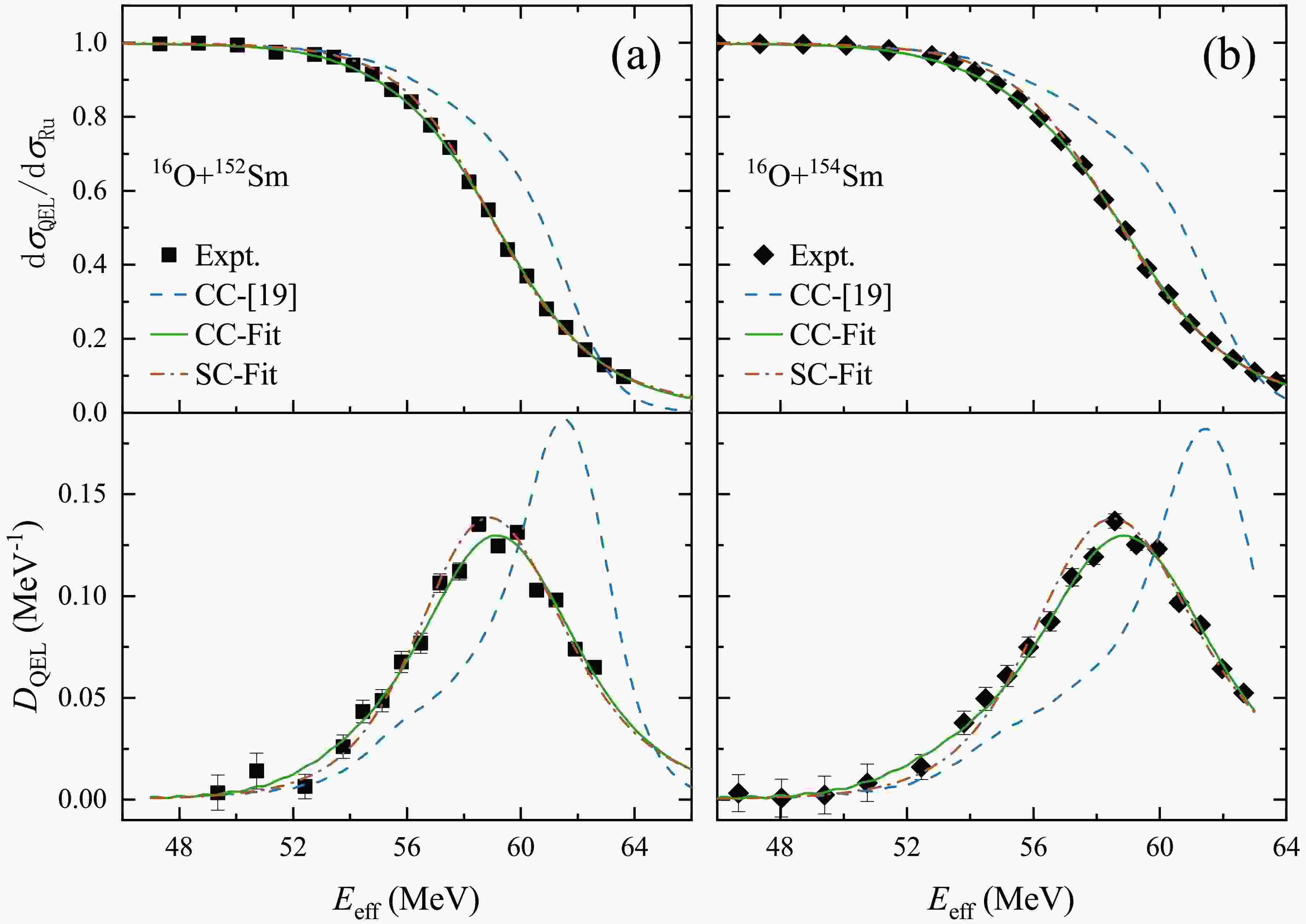
Samarium nuclei have long been a popular subject for studying nuclear properties due to their permanent deformation [34, 35, 36]. The best fit results for the CC and SC calculations of $ ^{16} $O $ +^{152,154} $Sm system are shown in Figure 1 (a) and (b), respectively. The specific values are shown in Table 3. It shows a long-range peculiarity. It can be seen that the results using imaginary part parameters in CC (solid line) and SC (dash-dot-dotted line) calculations well reproduced the experimental data with the theoretical deformation parameters and the real part nuclear potential. The result using the short range imaginary part potential (dashed line) in [19] already deviates from the experimental data at the energy region near the Coulomb barrier, and the peak position of the barrier distribution is shifted towards high energy region.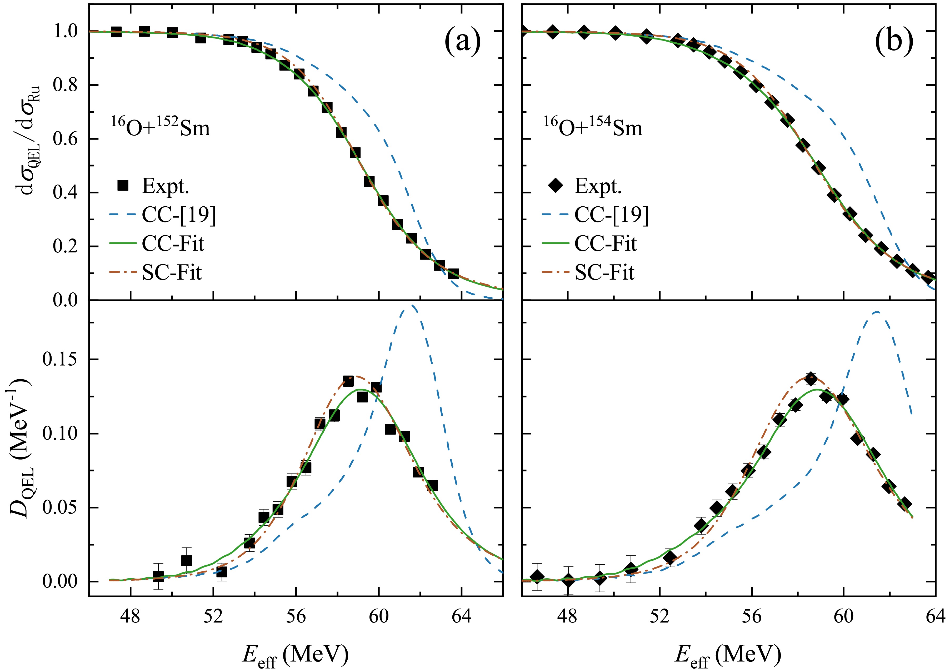

Figure 1.  (color online) Comparison of the experimental data with the fit results using the CC and SC calculations of $ ^{16} $O $ +^{152,154} $Sm systems and the calculation using the short range imaginary part potential in [19]. The dashed line is the calculation using the potential in [19], the solid and dash-dot-dotted lines are the calculations using the CC and SC fit result, respectively.

System	Method	W[MeV]	$ r_W $[fm]	$ a_W $[fm]	$ \chi^2_{\min}/\nu $
$ ^{16} $O+$ ^{152} $Sm	CC	$ 5.927\pm 0.707 $	$ 1.495\pm 0.005 $	$ 0.147\pm 0.011 $	2.37
	SC	$ 115.52\pm 31.29 $	$ 1.308\pm 0.009 $	$ 0.317\pm 0.009 $	5.46
$ ^{16} $O+$ ^{154} $Sm	CC	$ 4.566\pm 0.218 $	$ 1.525\pm 0.004 $	$ 0.058\pm 0.012 $	1.44
	SC	$ 91.84\pm 21.49 $	$ 1.325\pm 0.008 $	$ 0.319\pm 0.008 $	4.17
$ ^{16} $O+$ ^{184} $W	CC	$ 5.703\pm 0.343 $	$ 1.508\pm 0.004 $	$ 0.011\pm 0.001 $	0.87
	SC	$ 48.35\pm 20.47 $	$ 1.415\pm 0.007 $	$ 0.219\pm 0.007 $	3.10
$ ^{16} $O+$ ^{186} $W	CC	$ 6.107\pm 0.388 $	$ 1.509\pm 0.004 $	$ 0.064\pm 0.013 $	0.98
	SC	$ 60.44\pm 28.24 $	$ 1.402\pm 0.010 $	$ 0.236\pm 0.008 $	4.47

Table 3.  Best imaginary parameters W, $ r_W $ and $ a_W $ extracted from the CC and SC calculations, together with $ \chi^2 $ per degree of freedom of the best fit.

Tungsten nuclei are of interest because they lie in the region where the deformed rare-earth nuclei begin the transition toward the spherical nuclei near $ ^{208} $Pb. $ ^{152,154} $Sm, $ ^{184,186} $W all have positive $ \beta_2 $, but Sm isotopes have positive $ \beta_4 $ while W isotopes have negative $ \beta_4 $ for the ground-state rotational band. The comparison between the CC and SC results performed using the imaginary part potentials obtained from the best fit and the experimental data is presented in the Figure 2. Similar to the Sm case, it can be seen that the CC (solid line) and SC (dash-dot-dotted line) calculation results also reproduce well the experimental data for the theoretical deformation parameters and the real part nuclear potential. The results obtained with the short-range imaginary part potential (dashed line) in [19] have deviated from the experimental data in the energy region near the Coulomb barrier, and the peak position of the barrier distribution has shifted to the high-energy region.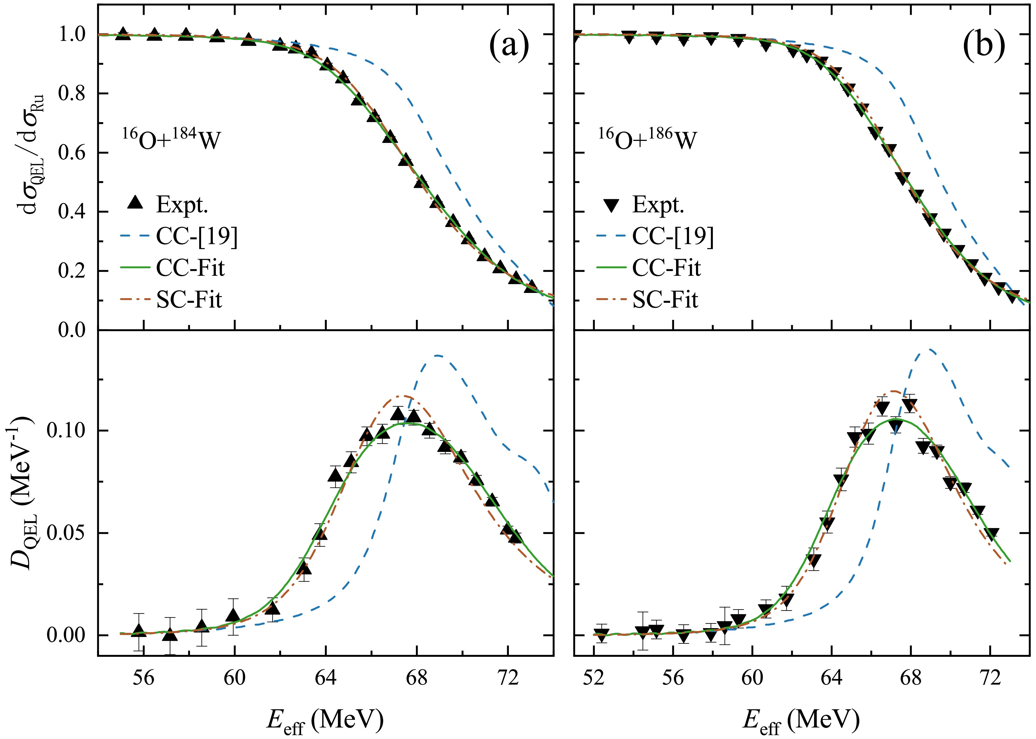

Figure 2.  (color online) The same as Figure 1 but for $ ^{16} $O+$ ^{184,186} $W reactions.

The specific values are shown in Table 3. The fit resultsfor both Sm and W are shallow long-range imaginary part potentials. It can be seen that the contrary sign of $ \beta_4 $ for Sm and W does not introduce obvious difference for the imaginary potential.

The imaginary part parameters W, $ r_W $ and $ a_W $ obtained from the best fits, with and without couplings are summarized in Table 3. The uncertainties in imaginary part potential parameter were calculated according to the following procedure [37]. Using the $ \chi^2 $ minimum value ($ \chi^2_{\min} $) corresponding to the best fit value of the imaginary part parameters, the quantity

was calculated, where $ {\rm{UP}}=3.53 $ for three-parameters fit [37], ν denotes the number of degrees of freedom. In the cases where $ \chi^2/\nu $ exceeded 1.5, the uncertainties on W, $ r_W $ and $ a_W $ were multiplied by $ \sqrt{\chi_{\min}^2/\nu} $ [14].

It can be seen from Table 3 that SC fits to the quasi-elastic scattering data give large imaginary part potential depth errors up to 30 MeV, while coupled channels analyses lead to values for W in the narrower range of the errors less than 1 MeV. Taking $ ^{16} $O+$ ^{152} $Sm as an example, the variation of the SC calculation results with varied W within its error are shown in the Figure 3 by the shadow grey area, with the fixed imaginary part potential parameters $ r_W $ and $ a_W $. It can be seen that the SC calculation result is not sensitive to the depth of the imaginary part potential.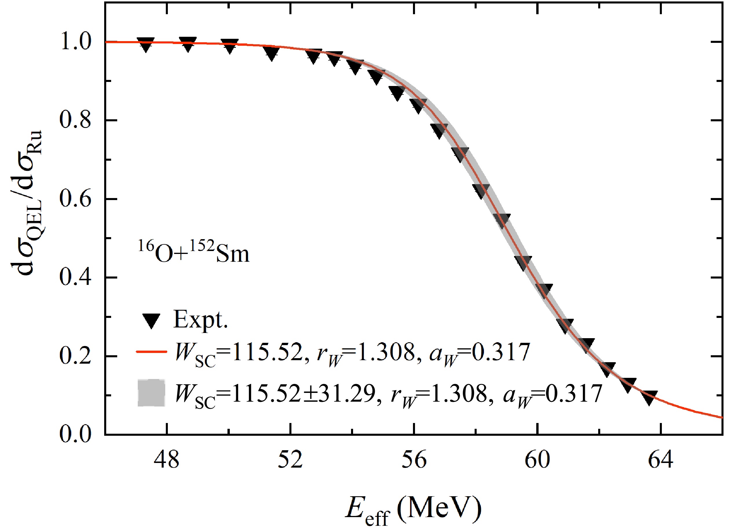

Figure 3.  (color online) Comparison of the experimental data and SC calculation for $ ^{16} $O$ +^{152} $Sm. The solid line and shadow gray area are the SC calculations using the best fit result of W, and its confidence level ($ 1\sigma $).

Comparison of the fitted potentials and the potential used in [19] for $ ^{16} $O+$ ^{186} $W is shown in Figure 4. According to Figure 4, the imaginary part potentials obtained by both SC and CC fit are longer-range than that used in [19]. The imaginary potential of CC extracted in the present work is different from that of SC. The imaginary potential extracted by CC is shallower and longer-range, and the coupling channel effect shows absorption, which corresponds to the enhancement of fusion cross sections below the barrier [21].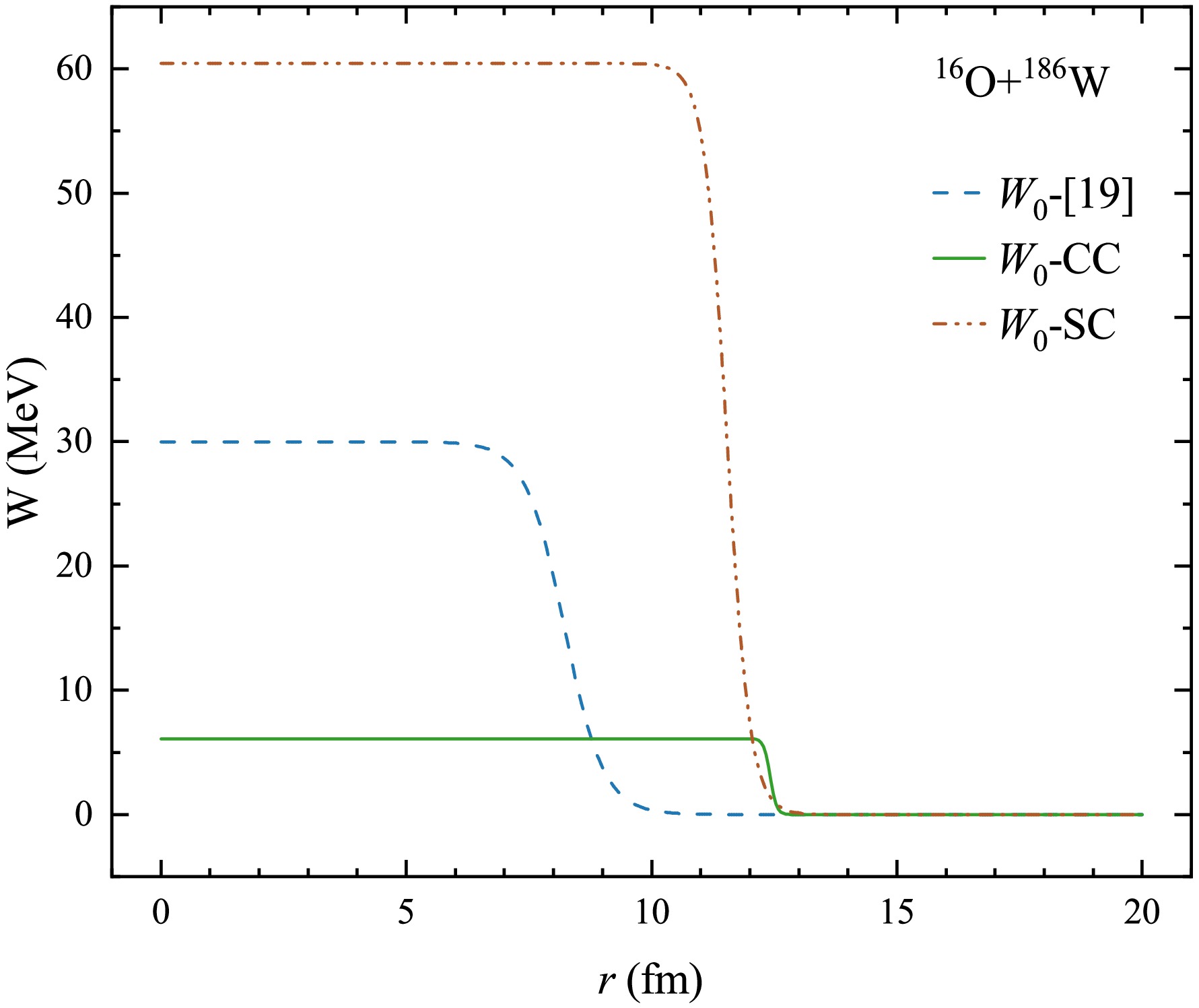

Figure 4.  (color online) Comparison of our fitted potentials and the potential used in [19] for $ ^{16} $O+$ ^{186} $W. The dashed line is the potential used in [19], the solid and dash-dot-dotted lines are the fitted potential using the CC and SC fit result, respectively.

Love et al [39] proposed that the strong couplinge effect could also be explained in terms of a long-range prefominantly imaginary dynamic polarisation potential (DPP) induced by the Coulomb coupling which, when added to a conventional optical model potential, provided a good description of $ ^{18} $O+$ ^{184} $W elastic scattering experimental angular distribution data at 90 MeV. For deformed nuclei, the long-range DPPs arise from the effect of the long-range Coulomb excitation of a rotational band, which is performed by a strongly depleted elastic scattering cross section [40, 35]. This also corresponds to the long-range imaginary part potential obtained in this work.

Since deformation is emphasized during fitting, a critical advantage of the extracted long-range imaginary potential lies in its ability to provide the possibility to extract deformation parameters across the whole energy range (sub- to above-barrier regions). The traditional short-range imaginary potential [19] is limited to the low energy region, where the Coulomb interaction is stronger and more sensitive to Coulomb deformation. In the previous work [22], the Coulomb deformation is usually treated as the same as the nuclear deformation, but in fact the Coulomb deformation is slightly larger than the nuclear deformation. Reproducing the backangle quasi-elastic excitation function over the whole energy region by the long-range imaginary part potential will help to extract the deformation parameters over the whole energy region, and can more realistically reflect the deformation of the nuclear material distribution. The systematic analysis of more deformed systems to obtain an appropriate imaginary part potential still needs to be completed, and the present work is only a preliminary attempt. It may provide a method to extract the deformation parameters for heavier systems that through the appropriate choice of imaginary potential.

The imaginary part potential parameters were extracted from the quasi-elastic scattering of $ ^{16} $O $ +^{152,154} $Sm, $ ^{184,186} $W using CC and SC calculations. It was found that the long range imaginary potential for the systems with well-deformed nuclei is needed for describing the experimental quasi-elastic scattering excitation function data in near-barrier energy region using CC calculations. Compared to the short-range imaginary part potential used in [19] for the sub-barrier data, the present results show that a long-range imaginary part potential is needed for backward quasi-elastic scattering at a wide energy region covering the Coulomb barrier. Considering the deformation effect, the long-range imaginary part potential obtained here reflects the strong absorption effect of the large deformation systems. In previous works, only a few effort [41, 42, 43, 44] have been made to reproduce simultaneously elastic scattering and fusion experimental data using the same potential. This finding is helpful to bridge the gap between fusion and scattering descriptions for well-deformed systems. Further systematic and more detailed studies with different projectile-target combinations from light to heavy systems are needed.