Gravitationally deformed polytropic models in extended teleparallel gravity and influence of decoupling parameters on constraining mass-radius relation

The construction of gravitational modifications, specifically extended theories of gravity, is motivated by both theoretical and observational factors. These modifications aim to encompass general relativity as a special case, but generally possess a more intricate and expansive structure [1]. One motivation is rooted in the non-renormalizability of general relativity (GR). It is hoped that by exploring more intricate extensions of GR, the issue of renormalizability could potentially be addressed and improved [2, 3]. Another motivation stems from the observed properties of the Universe, particularly the need to account for its two accelerated phases: one occurring during early times known as inflation, and another during late times referred to as the dark energy era. In constructing gravitational modifications, the conventional approach involves starting with the Einstein-Hilbert action and subsequently extending it through various methods [4]. However, an alternative approach is to begin with the torsional formulation of gravity, specifically the Teleparallel Equivalent of GR (TEGR) [5, 6], and introduce modifications accordingly. This leads to theories such as $ f({\cal{T}}) $ gravity [7−9], $ f({\cal{T}}, T_G) $ gravity [10], $ f({\cal{T}}, B) $ gravity [11, 12], scalar-torsion theories [15−17], etc. On the other hand, if we extend the gravitational action by introducing terms of the form $ f(R) $ or $ f({\cal{T}}) $, where f is a non-linear function, the resulting theories of gravity based on curvature or torsion exhibit substantial disparities. These theories are all inspired by the fundamental nature and principles of the gravitational field (see Refs. [12−14] for detailed reviews).

The extensively studied $ f(R) $ gravity, which relies on curvature, has been the subject of thorough examination in the previous decades [18]. One of the standout features of $ f(R) $ gravity is that its equations of motion involve fourth-order derivatives of the metric, which makes it fundamentally different from GR's second-order equations. This difference isn't just mathematical—it leads to modified versions of the Friedmann equations that can explain the accelerated expansion of the universe without needing to introduce dark energy [19]. When it comes to how theory is developed, researchers take a few different paths. The most common is the metric formalism, where the equations are derived by varying the action with respect to the metric alone [18]. Another approach is the metric-affine formalism (also known as the Palatini formalism), where both the metric and the connection are treated as separate variables [20]. There is also a more flexible hybrid formalism [21, 22], which blends ideas from both methods to create a broader framework for understanding how gravity might work beyond Einstein’s theory. An extension of $ f(R) $ gravity is $ f(R,{\cal{T}}) $ gravity, where the Lagrangian depends on both the Ricci scalar R and the trace of the EMT $ {\cal{T}} $ [23]. The T-dependence may stem from quantum effects or models of interacting dark energy [24]. This coupling leads to non-conservation of the EMT and introduces an extra force, causing test particles to deviate from geodesic motion. For more on its applications, see [25]. In cosmology, $ f(R,{\cal{T}}) $ gravity has been applied to the reconstruction of various models [26], including those based on holographic dark energy [27], and to describe both matter-dominated and accelerated phases [28]. Studies have also addressed scalar perturbations [29], dynamical systems [30, 31], and higher-dimensional scenarios such as 5D models and thick brane solutions [32, 33]. A notable generalization involves including the contraction $ R_{\mu\nu}{\cal{T}}^{\mu\nu} $, which reduces to $ f(R) $ gravity when $ {\cal{T}} = 0 $ [34, 35]. Astrophysically, $ f(R,{\cal{T}}) $ gravity and others have been explored in the context of dark matter [36] and compact objects [37−48].

In sharp contrast to $ f(R) $ gravity, the equations of motion in the torsion-based $ f({\cal{T}}) $ theory consist solely of the standard second-order derivatives of the tetrad fields, without the presence of higher-order derivatives. The properties of the $ f({\cal{T}}) $ theory have been extensively explored in the cosmological domain, as evidenced in numerous works; see, e.g., Refs. [9, 49−55]. Constraints on the theory have also been derived by analyzing the motion of planets in the Solar System, as indicated by relevant Refs. see, e.g., [57, 58]. However, investigations concerning static spherical symmetry, particularly in relation to stellar structure, are comparatively less abundant [59, 60]. The intrinsic characteristics of the theory of $ f({\cal{T}}) $ have been thoroughly examined, as documented in Refs.[61, 62]. Notably, an important challenge encountered in the early formulations of the theory is the absence of Lorentz invariance. This implies that the equations of motion generally do not exhibit invariance when different metric-compatible tetrad choices are made. This topic has been extensively discussed in the literature; see, e.g., Refs [63, 64]. Considerable efforts have been made in recent years to address and understand this problem. Several promising advances have been achieved through various approaches, including the Hamiltonian formalism [65], the null tetrad approach [66], the Lagrange multiplier formulation [67, 68], and the covariant formulation [16, 69]. These approaches have provided valuable insights and solutions to resolve the issue of Lorentz invariance in the $ f({\cal{T}}) $ theory.

In the theory of GR, the study of nonrotating stars is facilitated by employing static spherical symmetry and solving the well-known Tolman-Oppenheimer-Volkoff (TOV) equations. These equations provide the framework for constructing models of such stars. To fully characterize a star model, a matter model is also required, often utilizing a perfect fluid subject to an EOS. The energy density and pressure of the fluid can occupy the entire space. However, if they vanish strictly outside a finite spherical radius, the models represent compact stars enveloped by a vacuum. The phenomenology of these solutions is well understood within the framework of GR, offering a comprehensive understanding of their properties and behavior. The most notable achievements encompass the establishment of existence proofs for solutions involving certain classes of equations of state [70, 71], the derivation of upper bounds on the ratio of stellar mass to surface radius, which serves as an indicator of the compactness of compact objects [72, 73], and the exploration of the relationship between the curves describing the stellar mass to surface radius and the dynamical stability of the models [74].

In considering $ f({\cal{T}}) $ gravity as a more realistic framework for modeling stars, despite the success of $ f(R) $ gravity in explaining inflation and dark energy, a compelling motivation arises from the unique features and implications of $ f({\cal{T}}) $ gravity specifically related to compact objects. By incorporating torsion, which is a geometric quantity associated with the intrinsic angular momentum of matter, $ f({\cal{T}}) $ gravity introduces additional effects and interactions that allow for a more accurate representation of highly dense and strongly gravitating objects such as stars. This inclusion of torsion enables $ f({\cal{T}}) $ gravity to capture the intricate dynamics and behavior of stars with greater precision than $ f(R) $ gravity. Consequently, the modified field equations of $ f({\cal{T}}) $ gravity may yield distinct predictions regarding the structure, stability, and mass-radius relation of stars. Focusing on $ f({\cal{T}}) $ gravity facilitates the exploration of torsion-related effects that play a significant role in the behavior of stars, thereby offering a more comprehensive and realistic description. Moreover, the suitability of $ f({\cal{T}}) $ gravity in the modeling of stars is further reinforced by its consistency with relevant observational data, theoretical coherence, mathematical simplicity, and foundational aspects. These factors strengthen the argument for adopting $ f({\cal{T}}) $ gravity as an effective tool for understanding the properties and behavior of compact stellar objects. Notably, modified theories of gravity that incorporate torsion have been investigated in various applications. The study of relativistic stars was initially conducted by [59], while compact stars within a specific $ f({\cal{T}}) $ model for an isotropic fluid with a polytropic EOS were presented by [75]. Subsequently, the authors extended their analysis to include boson stars [76]. These studies exemplify the wide range of applications and the potential of $ f({\cal{T}}) $ gravity in comprehending the properties and behavior of compact stellar objects. Building upon these motivations, our paper introduces a groundbreaking contribution by introducing a novel exact solution for an anisotropic spherical model within the framework of $ f({\cal{T}}) $ gravity. To accomplish this, we exploit the well-known methodology of gravitational decoupling (GD) via the minimal geometric deformation (MGD) approach. This approach, combined with the utilization of a polytropic fluid source, allows us to accurately capture the intricate dynamics of the system. Additionally, we employ a well-behaved ansatz known as the Buchdahl metric ansatz for the radial component of the metric function. By incorporating these established techniques, we can derive a comprehensive and robust solution that significantly enhances our understanding of the behavior and properties of the system in the context of $ f({\cal{T}}) $ gravity.

Recent investigations have incorporated the concept of GD into the Einstein-Gauss-Bonnet (EGB) framework. Similarly to its role in the standard 4D classical gravity theory, GD facilitates the anisotropization of seed solutions, thus providing a mechanism to study the effects of anisotropic stresses in compact objects. The MGD method [77] was employed to model a compact star in 5D EGB gravity [78]. This approach demonstrated that the combined effects of the decoupling parameter and the EGB constant result in higher neutron star masses. Building on this, the extended MGD methodology [79] was utilized to derive an exact solution for a compact star within the 5D EGB gravity framework by [80]. There has been extensive research on modeling compact objects, such as NSTRs and strange stars, using MGD and complete geometric deformation (CGD). For a comprehensive overview of the applications of GD in astrophysics, the readers are referred to these references and the works cited within [81−85]. In particular, some pioneering studies on GD are also highlighted in these references [86−90].

The paper is organized as follows: It begins with a concise overview of the mathematical framework of $ f({\cal{T}}) $ gravity with an additional source in Section II. Section III then addresses the minimally gravitationally decoupled solution in $ f({\cal{T}}) $ gravity. The expressions for the model parameter, derived from the smooth matching conditions at the stellar surface, are discussed in Section IV. Section V presents the deformed strange star models and their relevance to astrophysics. The mass-radius relation for minimally deformed strange star models and their astrophysical relevance are explored in Section VI. The stability of our constructed deformed strange star model is discussed in Section VII via the adiabatic index and the HZN stability criterion. The measurement of the mass of a deformed anisotropic strange star via various planes is analyzed in Section VIII. The paper concludes with final remarks in Section IX.

The fundamental presumptions of $ f({\cal{T}}) $ gravity will now be discussed in this section. A vierbein field $ e_i(x^{\mu}) $, $ i = 0, 1, 2, 3, $ that serves as an orthonormal basis for the tangent space at every point $ x^{\mu} $ within the manifold is used as the dynamical object in teleparallelism. Every vector $ e_{i} $ can be characterized in a coordinate basis by its components $ e^{\mu}_{i} $, i.e., $ e_{i}=e^{\mu}_{i} \partial_{\mu} $ where $ \mu=0,1,2,3 $. We assume a particular convention and terminology: the Greek indices represent the coordinates of the space-time manifold, while the Latin indices indicate the components of the tangent space corresponding to the manifold (space-time). For any given space-time metric, we express the line element as follows: $ ds^2 = g_{\mu\nu} dx^{\mu}dx^{\nu} $=$ \eta_{ij}e^i_{\mu}e^j_{\nu}dx^{\mu}dx^{\nu} $, where $ \eta_{ij}=(-1,+1,+1,+1) $ is known as the Minkowski metric. Unlike general relativity (GR) which employs the Levi-Civita connection without torsion, Teleparallelism utilizes the Weitzenb$ \ddot{\text{o}} $ck connection $ \widehat{\gamma}_{\,\,\,\,\nu\mu}^{\lambda}=e^{\lambda}_{\,\,A}\partial_{\mu}e^A_{\,\,\,\nu} $, [91] which possesses a curvature-less torsion-based geometry. The torsion tensor can be defined as:

The general relativity is a metric theory of gravity and is torsion-free, that is $ {\cal{T}}^{\lambda}_{\; \; \; \mu\nu}=0 $. A common convention is to denote $ U_4 $ as a 4-dimensional space-time manifold equipped with both metric and torsion. Manifolds possessing a metric but lacking torsion are denoted as $ V_4 $ [92]. In many calculations, torsion often emerges in linear combinations, as seen in the contortion tensor, defined as:

We also introduce the skew-symmetric tensor $ {\cal{S}}_{\rho}^{\; \; \; \mu\nu} $ has the following form

The teleparallel Lagrangian, which serves as the torsion scalar, can be formulated using these quantities as [93]:

In this framework, the torsion tensor $ {\cal{T}}^{\lambda}_{\; \; \; \mu\nu} $ encapsulates all the information of the gravitational field, similar to how Riemann curvature tensor gives rise to the curvature scalar $ {\cal{R}} $ in GR. Consequently, the torsion scalar $ {\cal{T}} $ emerges from the torsion tensor in a parallel manner. In the teleparallel equivalent of General Relativity (TEGR), the action is expressed as $ {\cal{T}} $. However, the concept behind $ f({\cal{T}}) $ gravity is to extend $ {\cal{T}} $ into a function $ f({\cal{T}}) $. This mirrors the approach seen in GR, where the Ricci scalar $ {\cal{R}} $ in the Einstein-Hilbert action is generalized into a function $ f({\cal{R}}) $ that defines $ f({\cal{R}}) $ gravity [94]. The E-H action can be expressed as :

where, we have considered $ G=c=1 $ in the geometrized units and $ g=\text{det}(g_{\mu\nu}) $. $ {\cal{L_{\text{M}}}} $ denotes the Lagrangian density governing matter fields, linked to the energy momentum tensor (EMT) $ T_{\mu\nu} $, while $ {\cal{L_{{\Theta}}}} $ represents the Lagrangian density pertaining to the novel gravitational sector, often termed the "Θ gravitational sector" $ \Theta_{\mu\nu} $. This additional gravitational contribution consistently facilitates adjustments to matter fields within the $ f({\cal{T}}) $ gravity, and it can be integrated as part of the effective EMT $ T_{\mu\nu}^{\text{eff}}=T_{\mu\nu}+ \alpha \; \Theta_{\mu\nu} $. Here, α denotes the coupling constant that characterizes the interaction between the matter fields and the gravitational sector Θ. By varying the action (5) with respect to the vierbein, one can get the equation of motion as :

Where, $ \big\{T_{\rho}^{\; \; \nu}\big\}^{\text{eff}}=T_{\rho}^{\; \nu}+ \Theta_{\rho}^{\; \nu} $, $ f_{{\cal{T}}}=\dfrac{\partial f}{\partial {\cal{T}}} $ and $ f_{{\cal{T}}{\cal{T}}}=\dfrac{\partial^{2} f}{\partial {\cal{T}}^2} $.

The equations of motion within $ f({\cal{T}}) $-gravity can be reformulated utilizing the covariant derivative formalism as follows.

In this context, the Einstein tensor, denoted by $ G_{\nu\rho} $, enables the reformulation of Equation (7) within the framework of GR and the field equations associated with $ f({\cal{T}}) $ gravity as

here, $ {\cal{T}}_{\nu\rho}^{[{\cal{T}}]} $ represents a tensor incorporating adjustments arising from the torsion scalar, which is expressed as follows:

Now, the effective EMT in an anisotropic fluid distribution can be characterized as:

In this context, $ \rho^{\text {eff }} $ represents the effective energy density, $ p_r^{\text{eff}} $ denotes the fluid pressure along the radial direction relative to the four-velocity vector of time like $ {\cal{U}}_{{\nu}} $ (referred to as radial pressure), and $ p_t^{\text {eff }} $ signifies the orthogonal pressure to $ {\cal{U}}^{{\rho}} $ (known as tangential pressure). $ {\cal{U}}_{{\nu}} $ represents the four-velocity vector in the time-like direction, while $ {\cal{V}}_{{\nu}} $ indicates the unit space-like vector aligned with the radial coordinate direction. Therefore, we characterize dense matter using an anisotropic fluid, with the components of effective EMT given by $ \big(-\rho^{\text{eff}},p_r^{\text{eff}},p_t^{\text{eff}},p_t^{\text{eff}}\big) $. The effective components in the EMT can be written as,

Regarding the effective term, the appropriate anisotropy factor is,

It's notable that within the current anisotropic compact stellar system, there exist two distinct forms of anisotropies: $ T_{\mu\nu} $ and $ \Theta_{\mu\nu} $. Furthermore, another form of anisotropy, $ \Delta_{\Theta} $, becomes relevant due to GD, which plays a distinct role in transformation processes. Now, let us emphasize the interior of a spherically symmetric static fluid distribution, where the following line element specifies the space-time as :

This expression yields the distance formula $ dS^2=g_{ij}dx^{i}dx^{j} $, where $ x^{i}=(t,r,\Theta,\phi) $ represents the components of four-dimensional space-time, and $ {\cal{A}}(r) $ and $ {\cal{B}}(r) $ denote the static metric potentials along the time and radial coordinates, respectively. The expression for the torsion scalar and its derivative, expressed in terms of the radial coordinate, r, is given by

Now, for the metric (44), the tetrad matrix could be written as

Substituting the aforementioned tetrad field (16) and incorporating the torsion scalar along with its derivative into Eq. (6), it is possible to explicitly calculate the equations of motion for an anisotropic fluid in $ f({\cal{T}}) $ gravity in the following way:

The field equations discussed above (17-19) directly yield the equivalent field equations in GR when considering $ f({\cal{T}})={\cal{T}} $. However, in the context of $ f({\cal{T}}) $ gravity, an additional non-diagonal quantity emerges as follows:

Now, from the above Eq.(20) we get:

• Case I : $ {\cal{T}}^{\prime}=0 $ $ \Rightarrow {\cal{T}}=\text{constant}={\cal{T}}_0 $ i.e. $ {\cal{T}} $ is independent of r and hence $ {{\cal{T}}} $, $ f_{{\cal{T}}{\cal{T}}} $ remains constant.

• Case II : $ f_{{\cal{T}}{\cal{T}}}=0 $, which gives f as a linear function of two model parameters $ \zeta_1 $ and $ \zeta_2 $ that is, $ f({\cal{T}})=\zeta_1 {\cal{T}}+\zeta_2 $.

The linear functional mentioned above has been successfully employed in various other scenarios within $ f({\cal{T}}) $ gravity. Our objective now is to address the solution of the $ f({\cal{T}}) $ gravity field equations (17-19) in the functional form $ f({\cal{T}})=\zeta_1 {\cal{T}}+\zeta_2 $. To achieve this goal, we aim to utilize the well-known methodology known as GD via the MGD approach, employing a polytropic fluid source.

Now, inserting equation (14) and the form of $ f({\cal{T}}) $ into (17-19) we can obtained the equation of motion as follows:

Now, one can derive the conservation equation by requiring the effective stress-energy tensor to exhibit continuity, i.e. the divergence of the effective stress-energy tensor equals zero $ \Big(\nabla_{i}\big[T_j^{i}\big]^{\text{eff}}=0\Big) $, which gives,

It is important to note that equation (24) corresponds to the familiar Tolman-Oppenheimer-Volkoff (TOV) equation governing the decoupling system [95−97]. The TOV equations, derived from gravitational theory, serve to model the structure of spherically symmetrical objects that are in hydrostatic equilibrium. We observe that the perfect-fluid equations for $ f({\cal{T}}) $ gravity are formally regained as $ \alpha \to 0 $. Thus, we aim to utilize the GD under the MGD technique concerning the proposed compact star model to obtain the solution for the system of equation (21-23). We will observe that through this approach, the system will transform such that the equations of motion linked with the source $ \Theta^{\mu}_{{\cal{\nu}}} $ will meet to an effective "quasi-$ f({\cal{T}}) $ system". Now let us implement the geometric deformation that undergoes by the perfect fluid geometry namely :

Here, Φ and $ \psi(r) $ represent the geometric distortions experienced by the temporal and radial metric components, respectively. Among all the options outlined in Eqs. (26) and (27), there exists a particular one known as the MGD, for which $ \Phi(r)\to 0 $, thus the metric in (26) and (27) is minimally deformed by,

It is important to emphasize that the expression in Eq. (29) is a linear combination of the inverse radial metric component $ g_{11} $ in terms of a pure ideal fluid sector along with a contribution from the source $ \Theta_{\mu\nu} $. Let us now insert the components of equation (28) and (29) into the field equations (21-23). Consequently, the system is split into two sets:

• The normal field equations for a perfect fluid $ (\alpha=0) $ in gravity $ f({\cal{T}}) $, where the components of the systems are $ \big\{\rho, p_r, p_t, G(r), H(r)\big\} $.

• Another set of equation corresponding to the source $ \Theta_{\mu\nu} $ that has the components $ \big\{\rho, p_r, p_t, G(r), \psi(r)\big\} $is given by,

Under such circumstances, if we consider that there exists no transfer of energy-momentum between the perfect fluid $ (T_{\mu\nu}) $ and the source $ \Theta_{\mu\nu} $; their interaction is solely gravitational, then Eq.(25) explicitly yields,

These are referred to as the improved TOV equations for pure $ f({\cal{T}}) $ gravity and the Θ gravitational sector resulting from $ \nabla_{\mu}T^{\mu\nu}=0. $ and $ \nabla_{\mu}\Theta^{\mu\nu}=0 $ respectively. Several notable characteristics are related to the system (33-35). The primary similarity between it and conventional spherically symmetric field equations in $ f({\cal{T}}) $ gravity for an anisotropic system characterized by an EMT $ \Theta_{\mu\nu} $; $ \big\{\rho=\Theta_0^0, p_r=\Theta_1^1, p_t=\Theta_2^2 \big\} $ and its conservation equation is that they exhibit significant similarity. Furthermore, the active gravitational mass function for two systems may be expressed as:

In the framework of $ f({\cal{T}}) $ gravity, the pertinent mass functions for the sources $ T_{\mu\nu} $ and $ \Theta_{\mu\nu} $ are denoted as $ {\cal{M}}_{{\cal{T}}}(r) $ and $ {\cal{M}}_{\Theta}(r) $, respectively. Subsequently, within the context of minimally deformed spacetime, the interior mass function can be represented as

This section will examine the two sets of equations (21-23) and (33-35) about the sources $ T_{\mu\nu} $ and $ \Theta_{\mu\nu} $. The EMT $ T_{\mu\nu} $ indicates an anisotropic distribution of fluid matter; hence, $ \Theta_{\mu\nu} $ might enhance the overall anisotropy within the system, so facilitating the repulsion against gravitational collapse. Furthermore, an analysis of the second set of equations reveals that the resolution of the Θ sector is contingent upon the solution of the first system of equations. Therefore, it is advisable to resolve the original system first. The field equations are denoted by Eqs. Equations (21-23) are significantly non-linear, consisting of three equations and five unknowns $ \big\{\rho, p_r, p_t, G(r), H(r)\big\} $. To ascertain precise answers, one may separately choose any two of these variables. A method for obtaining precise solutions entails selecting one metric potential and imposing an extra assumption (such as a particular equation of state or embedding condition) to ascertain another metric potential. In our present work, we examine the quadratic polytropic equation of state defined as:

Here, γ, β, and χ represent constant parameters possessing appropriate dimensions, while n indicates the polytropic index. It should be noted that the polytropic EoS (40) can represent the EOS of the MIT bag when specific parameters are assigned, such as $ \gamma = 0,\; \beta = 1/4, $ and $ \chi = -4\,{\cal{B}}_g/3 $, where $ {\cal{B}}_g $ represents a constant in the bag [99]. Thus, the parameter γ assumes a significant role in revealing the nature of the contribution within the MIT bag model. Due to the high non-linearity in finding an exact solution, here we consider a polytropic index $ n=1 $. Under this choice, the EoS (40) is quadratic and the quadratic $ \gamma\rho^2 $ representing the neutron liquid in a Bose-Einstein condensate form. Meanwhile, the linear terms, $ \beta \rho+\chi $, come from the free-quarks model inherent in the popular MIT bag model for $ \beta = 1/4, $ and $ \chi = -4\,{\cal{B}}_g/3 $. Consequently, these NSTRs are likely characterized as "hybrid stars."

Now, substituting the expression of density and radial pressure from equations (21)-(22) into the EoS (40) we get

There are two unknowns in equation (41) namely $ G(r) $ and $ H(r) $ correspond to $ g_{tt} $ and $ g_{rr} $ components, respectively. Consequently, there are two ways to find the exact solution, either by considering a suitable metric potential along the temporal components or a radial direction.

For the present study, we consider a well-known ansatz Buchdahl metric for $ H(r) $ as [102]:

Where, A is dimensionless and B is the parameter without dimension of the metric function $ \text{km}^{-2} $. The metric function and its radial derivative exhibit non-singularity at the center of the stellar structure, fulfilling the necessary condition i.e.

The most interesting characteristic of the Buchdahl solution is that the inner Schwarzschild solution may be retrieved for $ A=0 $, but for $ A=1 $, the hypersurfaces $ \{t = \text{constant}\} $ are flat. Moreover, assuming $ C = -A/R^2 $ allows for the retrieval of the Vaidya and Tikekar [103] solution, and for $ A = -2 $, one obtains the Durgapal and Bannerji [105] solution. Numerous authors [104, 106, 107] later demonstrated that it constituted a feasible physical solution and illustrated its applicability in classifying some previously established exact solutions.

Now, for the known $ H(r) $ we have a first-order non-linear differential equation in $ G(r) $ (41) for which we can obtain the solution for another metric potential $ G(r) $ as,

Here, $ {\cal{G}} $ represents an arbitrary constant of integration. By employing the expressions for $ G(r) $ and $ H(r) $, we derive the expressions for ρ, $ p_r $, and $ p_t $ as follows.

where,

The given equations (45-46) provide the full spacetime geometry for the initial solution. However, to address the Θ sector, it is necessary to determine the solution for the second set of equations (33-35). To solve the second set of equations, we propose utilizing well-established techniques, specifically: (i) mimicking the density constraint, where $ \rho=\Theta_0^0 $, and (ii) mimicking the radial pressure constraint, where $ p_r=\Theta_1^1 $. These well-known techniques are physically motivated and thoroughly elaborated in ref [77]. Furthermore, there are a few other well-known recent techniques to solve the second set of equations are given as: mimicking the seed density with the dark matter density profile, mimicking the mass functions of the seed system and new source, linear equation of state between θ-sector etc. But here we shall use the $ \rho=\Theta_0^0 $ and $ p_r=\Theta_1^1 $ procedure to solve the θ-sector.

To address the solution of Θ-sector, we replicate the seed density to $ \Theta_0^0 $ i.e. $ \rho=\Theta^0_0 $. From the equation (21) and (33) we get an ordinary differential equation in the deformation function $ \psi(r) $ as;

By using the known metric function $ H(r) $ from (42) we solved the above first order and first degree differential equation to get the deformation function as,

where $ C_1 $ is the integrating constant which is set to be zero for the sake of a non-singular solution.

Now, utilizing the above deformation function (50), we get the solution of Θ sector from (34-35) as,

In this technique, next, we are mimicking the radial pressure $ p_r $ to $ \Theta_1^1 $ i,e, $ p_r=\Theta^1_1 $. Therefore from the Eqs (22), (34) and utilizing (44) we get the deformation function as,

Where,

Using the above deformation function (53) we have determined the other solution of Θ components as $ \Theta^0_0 $ and $ \Theta^2_2 $ as given below:

For the long expression we have given the detailed expression of $ P_{t1}(r) $, $ \Theta_{22}(r) $, $ \psi_{11} $, $ {\cal{L}} $, $ \Theta_{00}(r) $, $ \psi_{33} $, $ {\cal{N}} $ and $ \Theta^{22}(r) $ in the Appendix.

An essential phenomenon in the study of stellar distributions involves the continuity conditions at the surface of the star (at $ r={\cal{R}}_{\Sigma} $) between the interior (where $ r<{\cal{R}}_{\Sigma} $) and exterior (where $ r>{\cal{R}}_{\Sigma} $) regions of space-time geometries. According to the analysis conducted by [59], when considering the off-diagonal component as presented in equation (20), the viable solutions within the framework of $ f({\cal{T}}) $ gravity are confined to the following two scenarios: $ {\cal{T}}^{\prime}=0, \,f_{{\cal{T}}{\cal{T}}}=0 $ which have been discussed in the previous section. They examined the constrained scenario where $ f_{{\cal{T}}{\cal{T}}}=0 $ or $ {\cal{T}}^{\prime} = 0 $, applying it to spherically symmetric static distributions with a diagonal tetrad as background formalism. Birkhoff's theorem states that within a spherically symmetric vacuum, the Schwarzschild metric represents the most comprehensive solution according to the Einstein field equations. The Schwarzschild metric describes the gravitational field surrounding a spherical mass, under the assumption that the mass possesses zero electric charge, zero angular momentum, and there is no universal cosmological constant. Now we will briefly explain how an outer space-time metric for $ f({\cal{T}}) $ gravity could be determined. For the vacuum case, the EMT $ T_{\mu\nu}=0 $ so, in that case $ \rho=0,\,p_r=0,\,p_t=0 $. The first system of field equations (21),22 and (23) turns out to be,

Now, by integrating w.r.t r from the Eq.(55) one can get the form of the metric potential as

For the Schwarzschild solution $ {\cal{A}}(r),{\cal{B}}(r)\to 0 $ as $ r\to \infty $ which represents the flat space-time, constants $ b_0 $ must be zero. Now, for anti De-Sitter space-time metric (AdS$ _4 $), $ e^{{\cal{A}}(r)}=\sqrt{1+\frac{r^2}{a^2}} $ and $ e^{{\cal{B}}(r)}=\dfrac{1}{\sqrt{1+\frac{r^2}{a^2}}} $. Therefore, $ {\cal{A}}(r)=\dfrac{1}{2}\text{ln}\big(1+\dfrac{r^2}{a^2}\big) $ and $ {\cal{B}}(r)=-\dfrac{1}{2}\text{ln}\big(1+\dfrac{r^2}{a^2}\big) $, which imply $ {\cal{A}}(r)=\text{ln}(\dfrac{r}{a}) $ and $ {\cal{B}}(r)=-\text{ln}(\dfrac{r}{a}) $ as $ r \to \infty $ that is, in this limit, $ {\cal{A}}(r)+{\cal{B}}(r)=0 $ which gives $ \text{constant}=0 $, gives a similar result to the previous case as $ {\cal{A}}(r)=-{\cal{B}}(r) $. Now, by using Eq.(55) and (56) we get,

In the limit of small r values, the Newtonian approximation yields a constant value equal to $ 2{\cal{M}} $, where $ {\cal{M}} $ represents the active gravitational mass. Furthermore, one can note that the above space-time solution will represent the Schwarzschild anti-De-Sitter solution if we consider the cosmological constant $ \Lambda=-\dfrac{\zeta_2}{2\zeta_1} $ and const.$ =-2{\cal{M}} $ then,

Considering the preceding discussion, we select the Schwarzschild anti-de Sitter (SAdS$ _4 $) metric within the framework of $ f({\cal{T}}) $ gravity for describing the outer region of space-time as,

Moreover, the following line element provides the interior metric encompassing the geometric distortion as:

According to Israel-Darmois condition [108, 109], for the sake of ensuring a stable configuration, it is necessary to smoothly connect the inner manifold $ dS_{-}^2 $ (63) with the outer manifold $ dS_{+}^2 $ (62) at the boundary Σ. This entails employing a well-established continuity equation, which ultimately determines the first and second fundamental forms across the surface Σ by integrating both geometries at this boundary. Regarding the first fundamental form, the representation of the inner geometry through the metric tensor $ g_{\mu\nu} $, derived from $ dS_{-}^2 $ and $ dS_{+}^2 $ on the interface, can be described as follows:

Taking into account Eq.(63) and Eq.(62), it takes an explicit form as follows:

Alternatively, the second fundamental form assumes the following expression:

To compute the numerical values of the constants, we utilize equations (66),(67) and (68) to determine the unspecified parameters, including the constant $ {\cal{G}} $, mass ($ {\cal{M}} $), and polytropic constant χ.

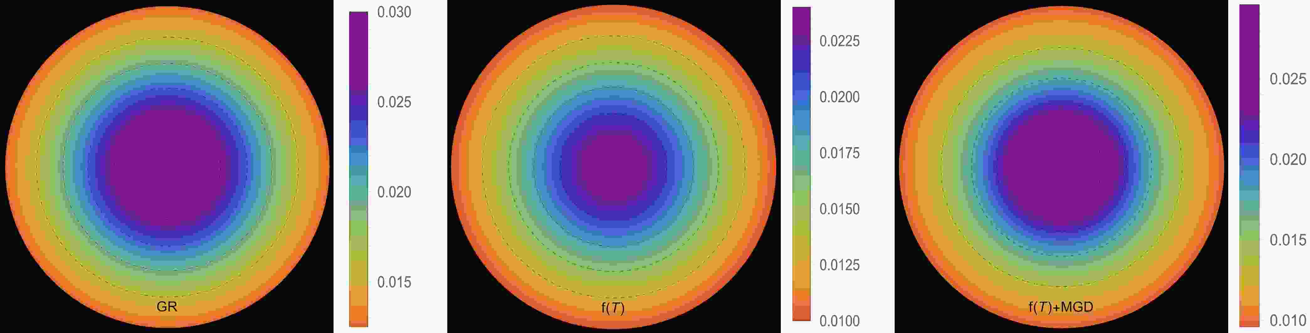
In this section, our focus will be on examining the physical viability of our deformed strange star models and their significance in the context of astrophysics. Specifically, we aim to analyze the behaviors of various thermodynamic variables, including effective energy density, effective radial and effective tangential stresses, and the effective anisotropic parameter. By scrutinizing these aspects, we aim to assess the relevance of these models in explaining astrophysical phenomena for both solutions: solution III A [$ \Theta^0_0=\rho $] and solution III B [$ \Theta^1_1=p_r $]. The effective energy density exhibits a consistent decreasing trend as a function of the radial coordinate, reaching its maximum value at the center of the self-gravitating object. This observation is demonstrated in Figs. 1 and 5. Notably, both figures illustrate that the effective energy density remains regular at every interior point of the configuration for all three scenarios: GR $ \big(\alpha=0.0 $, $ \zeta_1=1.0 $, $ \zeta_2=0.0 $ $ [\text{km}^{-2}]\big) $-left panel, $ f({\cal{T}}) $ $ \big(\alpha=0.0 $, $ \zeta_1=0.8 $, $ \zeta_2=2\times 10^{-6} $ $ [\text{km}^{-2}]\big) $-middle panel, and $ f({\cal{T}})+\text{MGD} $ $ \big(\alpha=0.2 $, $ \zeta_1=0.8 $, $ \zeta_2=2\times 10^{-6} $ $ [\text{km}^{-2}]\big) $-right panel. The primary distinction between Figs. 1 and 5 lies in the varying magnitudes of the three scenarios, despite having the same fixed parameters. We observe that in the scenario of GR, a higher core effective density is present with $ \zeta_1 $. However, in the scenario of $ f({\cal{T}}) $, a decrease in the magnitude of $ \zeta_1 $ and the presence of $ \zeta_2 $ lead to a lower core effective density. Conversely, in the $ f({\cal{T}})+\text{MGD} $ scenario, the inclusion of α enhances the effective density in the central regions of the star, resulting in a concentration of matter in central, concentric shells. However, as one moves away from the center towards the surface layers of the star, variations in α, $ \zeta_1 $, and $ \zeta_2 $ have no noticeable impact on the stellar effective density. In Figs. 2 and 3 along with 6, and 7, we present the distribution of effective radial and tangential pressures with respect to the radial coordinates. These figures allow us to analyze the variations in effective radial and tangential pressure among the three scenarios. In the solution presented in III A–(Figs. 2 and 3), where the initial condition is $ \Theta^0_0=\rho $, we can clearly see that the effective radial and tangential pressures in the central region are higher compared to the $ f({\cal{T}}) $ scenario. Furthermore, when the $ f({\cal{T}})+\text{MGD} $ scenario is considered, incorporating the MGD leads to even lower effective radial and tangential pressures. This observation strongly suggests that the presence of MGD has a confining and compacting effect on the fluid particles, particularly in the central regions of the star. In the solution presented in III B–(Figs. 6 and 7), where the initial condition is $ \Theta^1_1=p_r $, we observe a similar pattern to the effective density. Specifically, in the case of GR, we find that the effective radial and tangential pressures in the central region are higher compared to the $ f({\cal{T}}) $ scenario. Furthermore, when we include the MGD in the $ f({\cal{T}})+\text{MGD} $ scenario, the effective radial and tangential pressures increase even further. This indicates that the presence of MGD has a relaxing effect on the fluid particles, with this effect being particularly pronounced in the central regions of the star. Importantly, in both solutions, the effective radial and tangential pressures remain continuous throughout the star and exhibit a monotonically decreasing trend with increasing radial coordinates. It is worth noting that the effective radial component of the pressure at the stellar surface disappears, which is a significant characteristic observed in these solutions. Figs. 4 and 8 illustrate the trend of the effective anisotropy parameter, $ \Delta(r) $, for three distinct scenarios with the same fixed parameters in both solutions. It is worth noting that the presence of the MGD leads to a significant increase in the anisotropy within the stellar body compared to the cases of GR and $ f({\cal{T}}) $. Specifically, when comparing the scenarios of GR, $ f({\cal{T}}) $, and $ f({\cal{T}})+\text{MGD} $, we observe that the inclusion of MGD causes the anisotropy parameter to double. This finding highlights the pronounced impact of MGD on the anisotropic nature of the system, indicating that the presence of MGD significantly enhances the anisotropy within the stellar body. The observed amplification of anisotropy serves to reinforce the stability of the star's surface layers. The presence of the MGD plays a crucial role in inducing greater anisotropy within the stellar fluid by introducing a larger disparity between the radial and tangential stresses. This enhanced anisotropy, facilitated by MGD, can be attributed to various physical processes taking place within the stellar interior. These processes include phase transitions, the transport of neutrinos and electrons, as well as dissipation. Each of these mechanisms contributes to the overall increase in anisotropy. Phase transitions occurring within the stellar interior can result in changes to the EoS, affecting the balance between radial and tangential stresses. Neutrino and electron transport processes also influence the pressure distribution, leading to variations in anisotropy throughout the star. Dissipative effects, such as viscosity or heat conduction, can further contribute to the development of anisotropic stresses. It is intriguing to observe that the effective anisotropy, initially starting at zero at the center of the star, gradually grows in magnitude as we move towards the outer boundary. This increasing anisotropy is accompanied by a positive value of $ \Delta(r) $, indicating a repulsive force arising from radial stresses overpowering transverse stresses within the star. The mounting anisotropy and the resultant repulsive force play a significant role in enhancing the stability of the star's surface layers. They become crucial in counteracting the inward gravitational force, thereby contributing to the overall stability of the compact object. This interplay between increasing anisotropy, repulsive forces, and the counterbalance of gravitational forces is instrumental in maintaining the stability of the star's surface layers and ensuring the resilience of the compact object.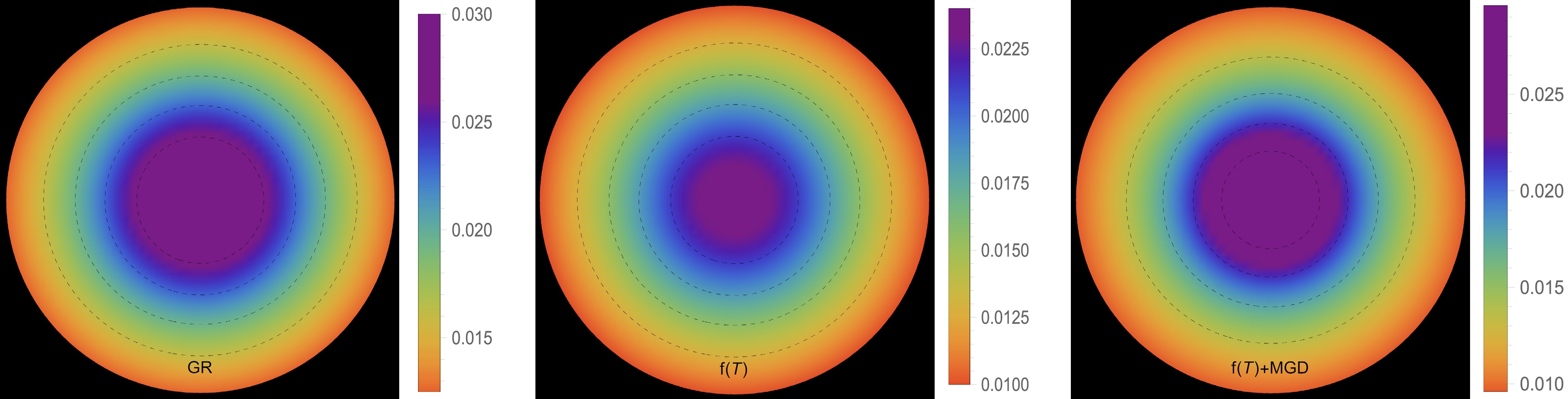

Figure 1.  (color online) The density profile [$ \rho^{\text{eff}}(r) $] in [$ \text{km}^{-2} $] along to the radial distance r of the stellar model for solution III A [$ \Theta^0_0=\rho $] in context of GR $\big( \alpha=0.0 $, $ \zeta_1=1.0 $, $ \zeta_2=0.0 $ $ [\text{km}^{-2}]\big) $-left panel, $ f({\cal{T}}) $ $ \big(\alpha=0.0 $, $ \zeta_1=0.8 $, $ \zeta_2=2\times 10^{-6} $ $ [\text{km}^{-2}]\big) $-middle panel, and $ f({\cal{T}})+\text{MGD} $ $\big( \alpha=0.2 $, $ \zeta_1=0.8 $, $ \zeta_2=2\times 10^{-6} $ $ [\text{km}^{-2}]\big) $-right panel. The fixed values of the constant parameters are: $ A = -1.5 $, $ B=0.006 $, $ \gamma=10 $, $ \beta=0.33 $, and $ R=11\; \text{km} $.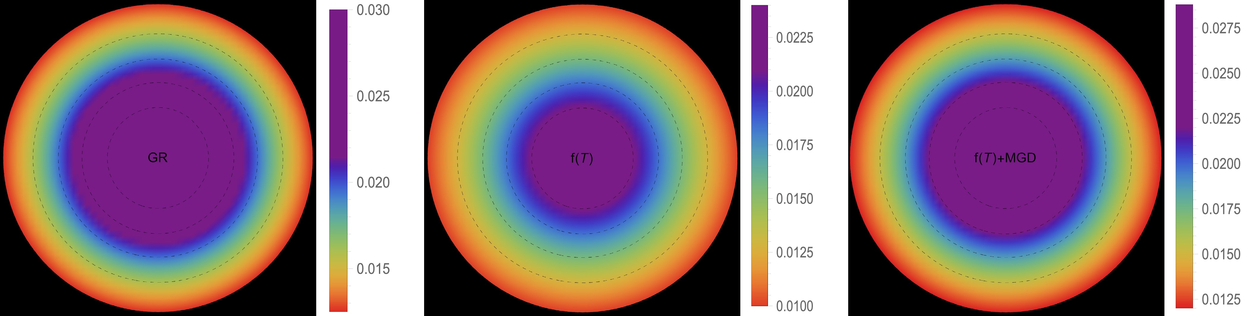

Figure 5.  (color online) The effective density profile [$ \rho^{\text{eff}}(r) $] in [$ \text{km}^{-2} $] along to the radial distance r of the stellar model for solution III B [$ \Theta^1_1=p_r $] in context of GR $\big( \alpha=0.0 $, $ \zeta_1=1.0 $, $ \zeta_2=0.0 $ $ [\text{km}^{-2}]\big) $-left panel, $ f({\cal{T}}) $ $ \big(\alpha=0.0 $, $ \zeta_1=0.8 $, $ \zeta_2=2\times 10^{-6} $ $ [\text{km}^{-2}]\big) $-middle panel, and $ f({\cal{T}})+\text{MGD} $ $\big( \alpha=0.2 $, $ \zeta_1=0.8 $, $ \zeta_2=2\times 10^{-6} $ $ [\text{km}^{-2}]\big) $-right panel.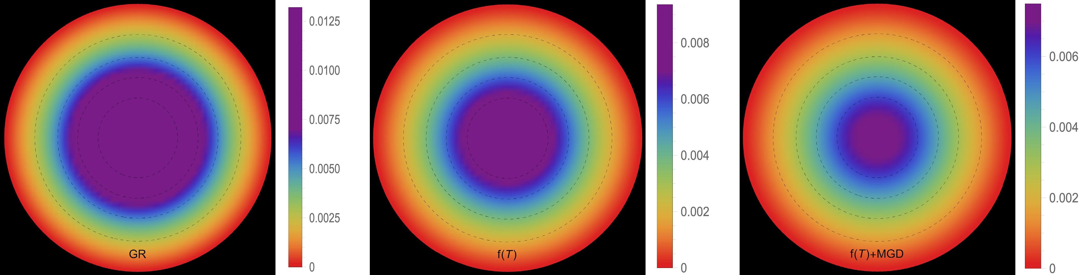

Figure 2.  (color online) The radial pressure profile [$ p^{\text{eff}}_r(r) $] in [$ \text{km}^{-2} $] along to the radial distance r of the stellar model for solution III A [$ \Theta^0_0=\rho $] in context of GR $\big( \alpha=0.0 $, $ \zeta_1=1.0 $, $ \zeta_2=0.0 $ $ [\text{km}^{-2}]\big) $-left panel, $ f({\cal{T}}) $ $ \big(\alpha=0.0 $, $ \zeta_1=0.8 $, $ \zeta_2=2\times 10^{-6} $ $ [\text{km}^{-2}]\big) $-middle panel, and $ f({\cal{T}})+\text{MGD} $ $\big( \alpha=0.2 $, $ \zeta_1=0.8 $, $ \zeta_2=2\times 10^{-6} $ $ [\text{km}^{-2}]\big) $-right panel.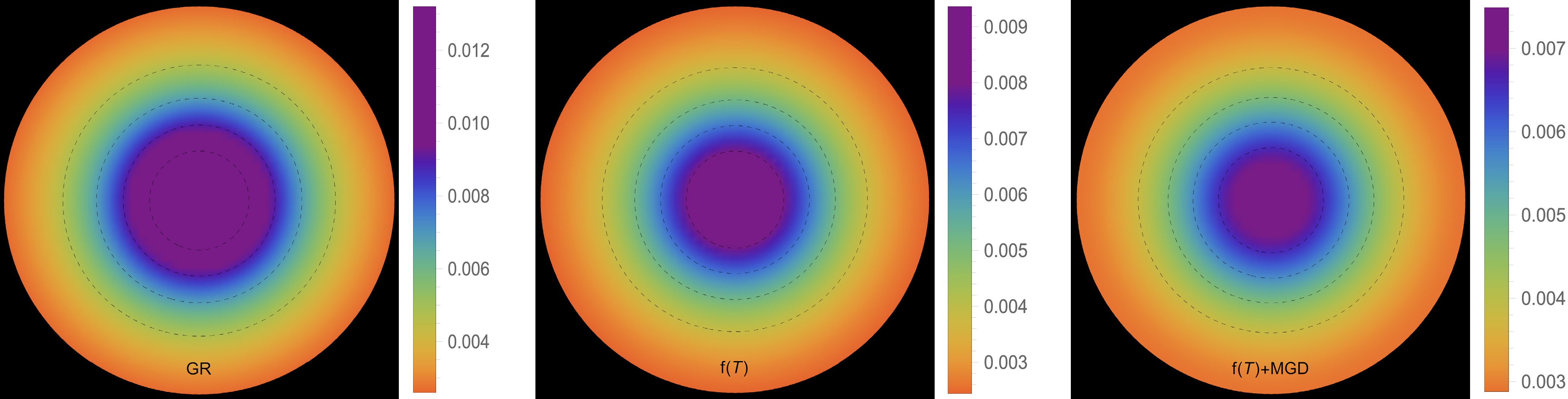

Figure 3.  (color online) The effective tangential pressure profile [$ p^{\text{eff}}_t(r) $] in [$ \text{km}^{-2} $] along to the radial distance r of the stellar model for solution III A [$ \Theta^0_0=\rho $] in context of GR $\big( \alpha=0.0 $, $ \zeta_1=1.0 $, $ \zeta_2=0.0 $ $ [\text{km}^{-2}]\big) $-left panel, $ f({\cal{T}}) $ $ \big(\alpha=0.0 $, $ \zeta_1=0.8 $, $ \zeta_2=2\times 10^{-6} $ $ [\text{km}^{-2}]\big) $-middle panel, and $ f({\cal{T}})+\text{MGD} $ $\big( \alpha=0.2 $, $ \zeta_1=0.8 $, $ \zeta_2=2\times 10^{-6} $ $ [\text{km}^{-2}]\big) $-right panel.

Figure 6.  (color online) The effective radial pressure profile [$ p^{\text{eff}}_r(r) $] in [$ \text{km}^{-2} $] along to the radial distance r of the stellar model for solution III B [$ \Theta^1_1=p_r $] in context of GR $\big( \alpha=0.0 $, $ \zeta_1=1.0 $, $ \zeta_2=0.0 $ $ [\text{km}^{-2}]\big) $-left panel, $ f({\cal{T}}) $ $ \big(\alpha=0.0 $, $ \zeta_1=0.8 $, $ \zeta_2=2\times 10^{-6} $ $ [\text{km}^{-2}]\big) $-middle panel, and $ f({\cal{T}})+\text{MGD} $ $\big( \alpha=0.2 $, $ \zeta_1=0.8 $, $ \zeta_2=2\times 10^{-6} $ $ [\text{km}^{-2}]\big) $-right panel.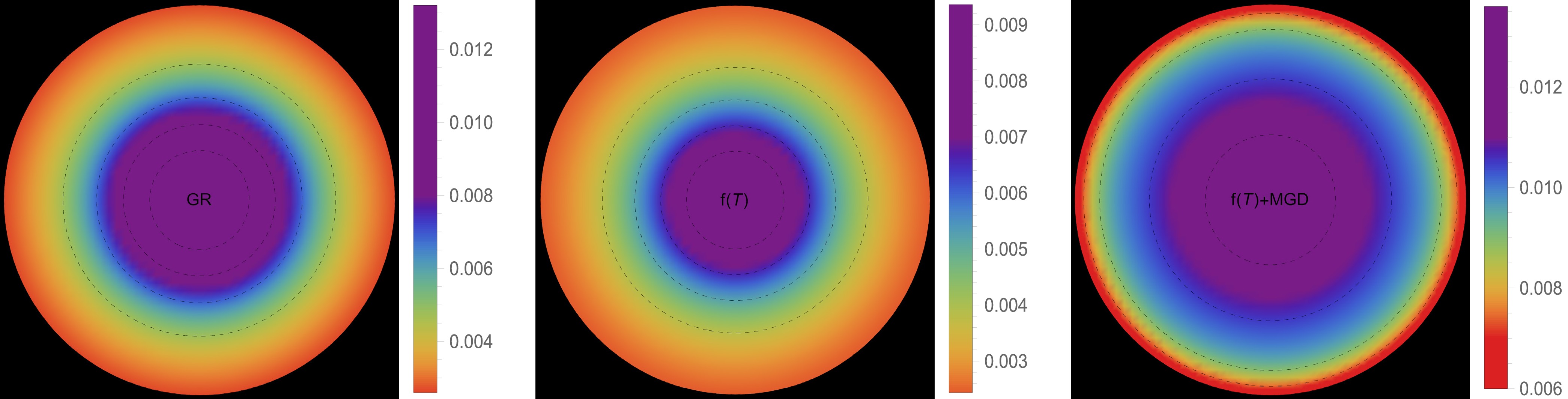

Figure 7.  (color online) The effective tangential pressure profile [$ p^{\text{eff}}_t(r) $] in [$ \text{km}^{-2} $] along to the radial distance r of the stellar model for solution III B [$ \Theta^1_1=p_r $] in context of GR $\big( \alpha=0.0 $, $ \zeta_1=1.0 $, $ \zeta_2=0.0 $ $ [\text{km}^{-2}]\big) $-left panel, $ f({\cal{T}}) $ $ \big(\alpha=0.0 $, $ \zeta_1=0.8 $, $ \zeta_2=2\times 10^{-6} $ $ [\text{km}^{-2}]\big) $-middle panel, and $ f({\cal{T}})+\text{MGD} $ $\big( \alpha=0.2 $, $ \zeta_1=0.8 $, $ \zeta_2=2\times 10^{-6} $ $ [\text{km}^{-2}]\big) $-right panel.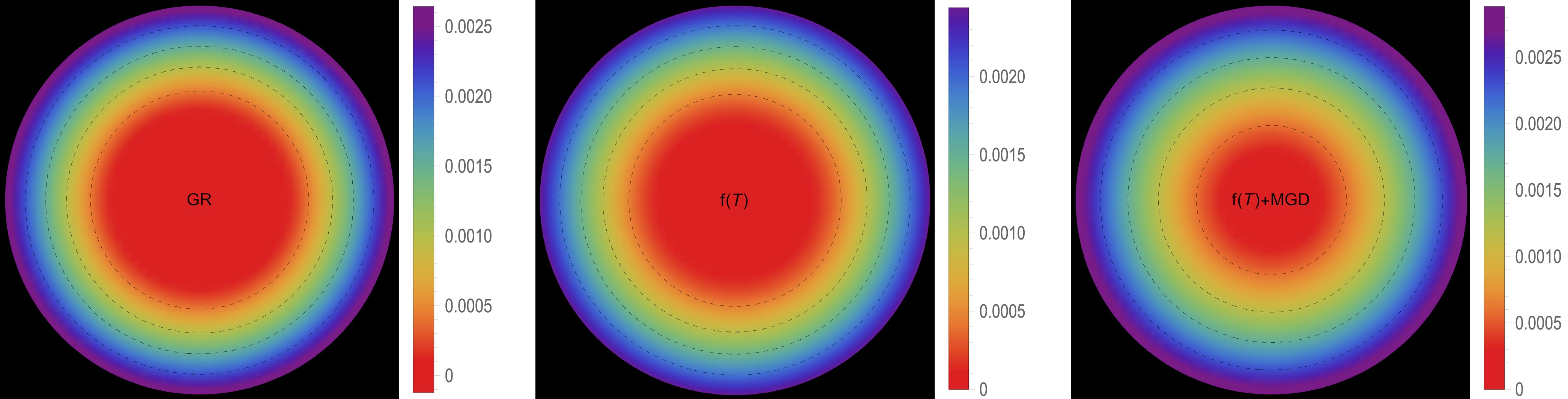

Figure 4.  (color online) The effective anisotropy profile [$ \Delta^{\text{eff}}(r) $] in [$ \text{km}^{-2} $] along to the radial distance r of the stellar model for solution III A [$ \Theta^0_0=\rho $] in context of GR $\big( \alpha=0.0 $, $ \zeta_1=1.0 $, $ \zeta_2=0.0 $ $ [\text{km}^{-2}]\big) $-left panel, $ f({\cal{T}}) $ $ \big(\alpha=0.0 $, $ \zeta_1=0.8 $, $ \zeta_2=2\times 10^{-6} $ $ [\text{km}^{-2}]\big) $-middle panel, and $ f({\cal{T}})+\text{MGD} $ $\big( \alpha=0.2 $, $ \zeta_1=0.8 $, $ \zeta_2=2\times 10^{-6} $ $ [\text{km}^{-2}]\big) $-right panel.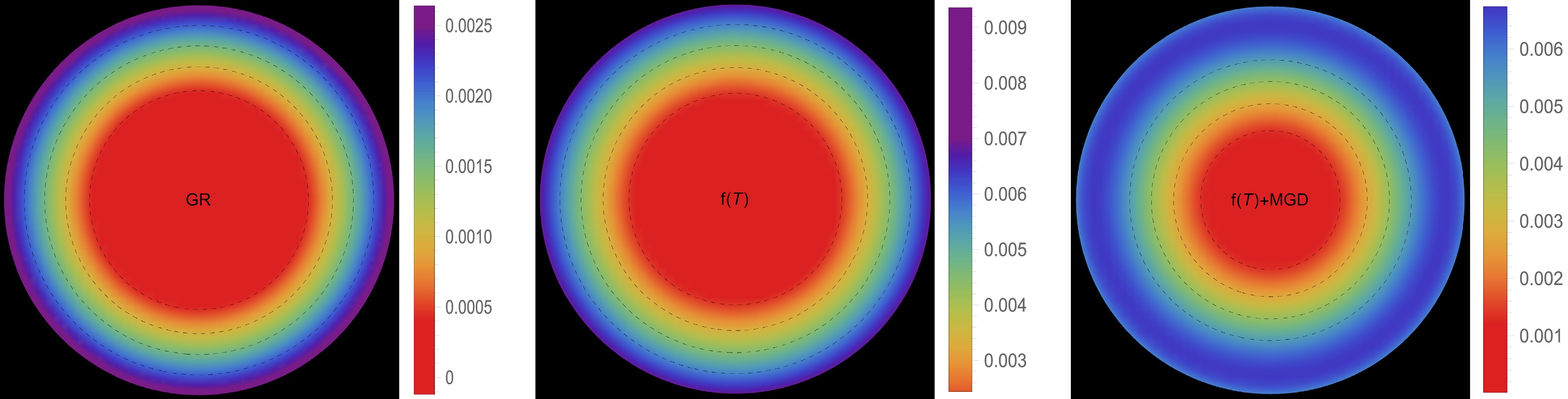

Figure 8.  (color online) The effective anisotropy profile [$ \Delta^{\text{eff}}(r) $] in [$ \text{km}^{-2} $] along to the radial distance r of the stellar model for solution III B [$ \Theta^1_1=p_r $] in context of GR $\big( \alpha=0.0 $, $ \zeta_1=1.0 $, $ \zeta_2=0.0 $ $ [\text{km}^{-2}]\big) $-left panel, $ f({\cal{T}}) $ $ \big(\alpha=0.0 $, $ \zeta_1=0.8 $, $ \zeta_2=2\times 10^{-6} $ $ [\text{km}^{-2}]\big) $-middle panel, and $ f({\cal{T}})+\text{MGD} $ $\big( \alpha=0.2 $, $ \zeta_1=0.8 $, $ \zeta_2=2\times 10^{-6} $ $ [\text{km}^{-2}]\big) $-right panel.

Pulsars are NSTRs that can emit periodic and strong electromagnetic signals as pulses arising from their high magnetic fields and rotational property. The large rotational frequencies exhibited by pulsars suggest that they possess a high degree of compactness. Typically, pulsars are found in binary systems, where a massive neutron star is accompanied by a companion star. By applying Kepler's third law, these binary systems can be used to measure the mass of the pulsar through the analysis of time delays in the observed pulses [110, 111].

Determining the radii of NSTRs is a challenging and complex task, as compared to measuring their masses. This difficulty arises due to various observational parameters involved in the process [112, 113]. However, recent advancements have provided new avenues for estimating neutron star radii. One method involves studying the tidal deformability factor, which is associated with the detection of gravitational waves [114]. Another approach utilizes measurements obtained from NICER (Neutron star Interior Composition Explorer) on hotspots located on the surfaces of NSTRs [115, 116]. These recent breakthroughs have opened up promising avenues for advancing our understanding of neutron star radii, offering new possibilities for precise measurements in the future.

In this study, we have developed a framework utilizing the well-known Buchdahl metric in $ f({\cal{T}}) $ gravity to construct models of pulsars. A key aspect of our analysis is the investigation of $ M-R $ curves, as depicted in Figures 9, 10, and 11. These curves represent different values of α, β, γ, and $ \zeta_1 $, for both Solution III A ($ \Theta^0_0=\rho $) and Solution III B ($ \Theta^1_1=p_r $). It is worth noting that the mass-radius curves are obtained using the quadratic polytropic EOS in conjunction with the TOV equation. This combination allows us to explore the relationship between mass and radius for pulsars within the context of our $ f({\cal{T}}) $ gravity framework. Figures 9, 10, and 11 also showcase the horizontal bands representing the selected pulsars. The $ M-R $ curves that intersect with constraints such as the black hole formation but do not intersect with the horizontal bands of pulsars can be excluded when measuring radii. This exclusion criterion facilitates the prediction of the radii listed in Tables 1, 2, and 3.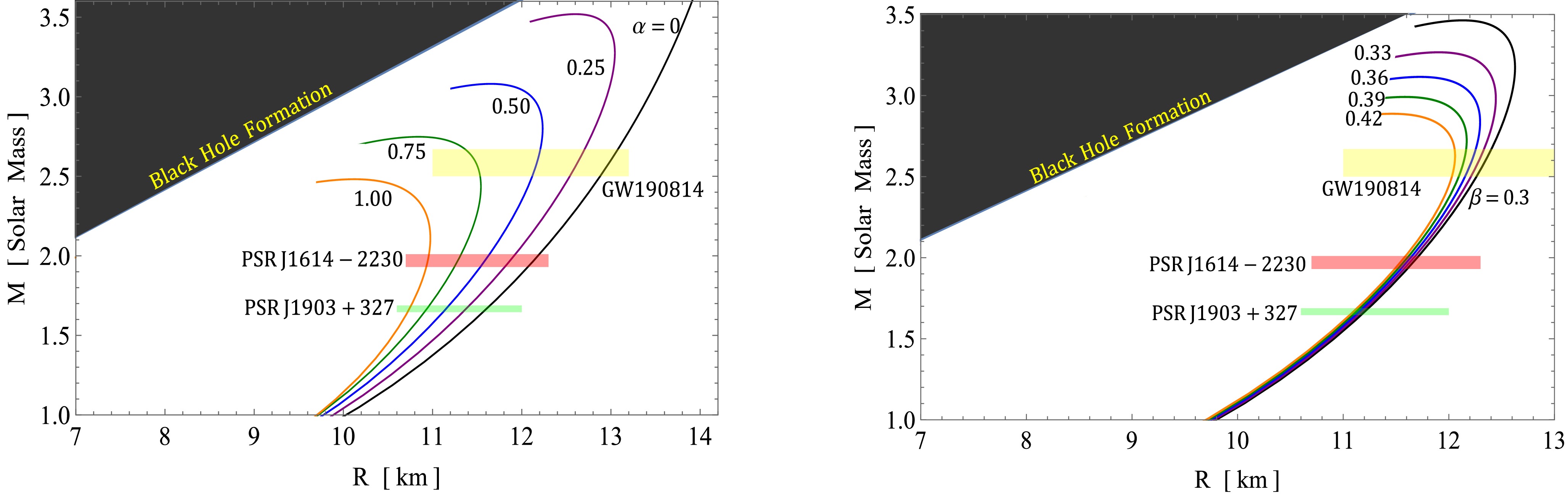

Figure 9.  (color online) The $ M-R $ curves for different free parameters values α-left panel with fixed $ \beta=0.33 $, $ \gamma=20 $, $ \zeta_1= 0.5 $ and right figure shows the $ M-R $ curves for different β with fixed $ \alpha=0.5 $, $ \gamma=15 $, and $ \zeta_1=0.5 $. The both figures represent the mass-radius relation for solution III A $ \left[\Theta^0_0=\rho\right] $.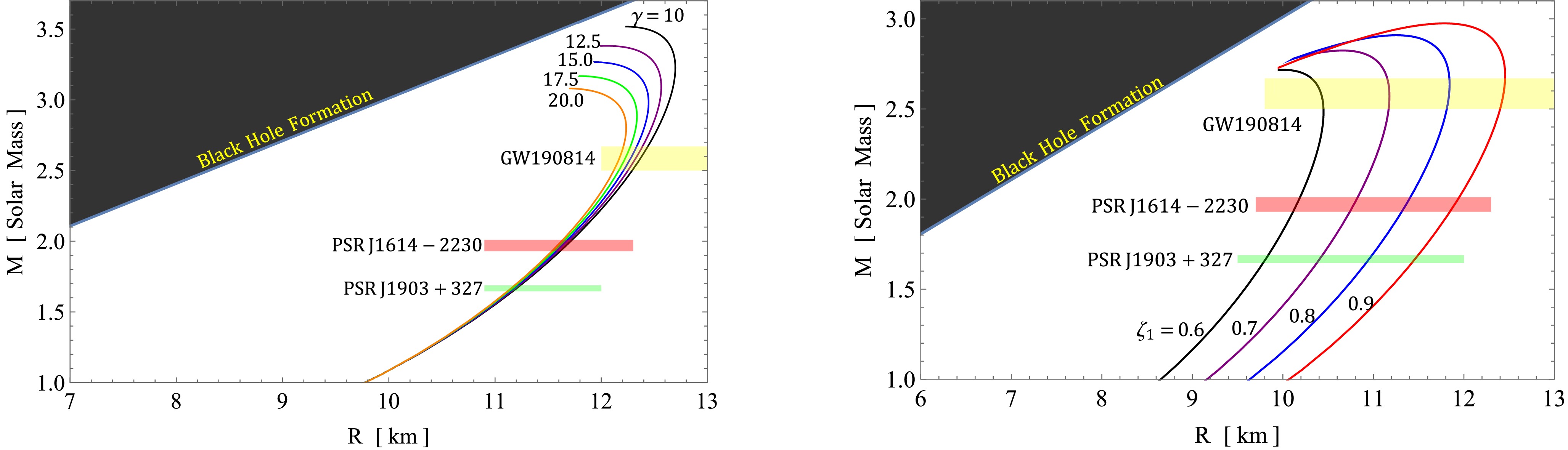

Figure 10.  (color online) The $ M-R $ curves for different free parameters values γ-left panel with fixed $ \beta=0.33 $, $ \alpha==0.5km^2 $, $ \zeta_1=0.5 $ and right figure shows the $ M-R $ curves for different $ \zeta_1 $ with fixed $ \alpha=0.5 $, $ \gamma=15 $, and $ \beta=0.33 $. The both figures represent the mass-radius relation for solution III A $ \left[\Theta^0_0=\rho\right] $.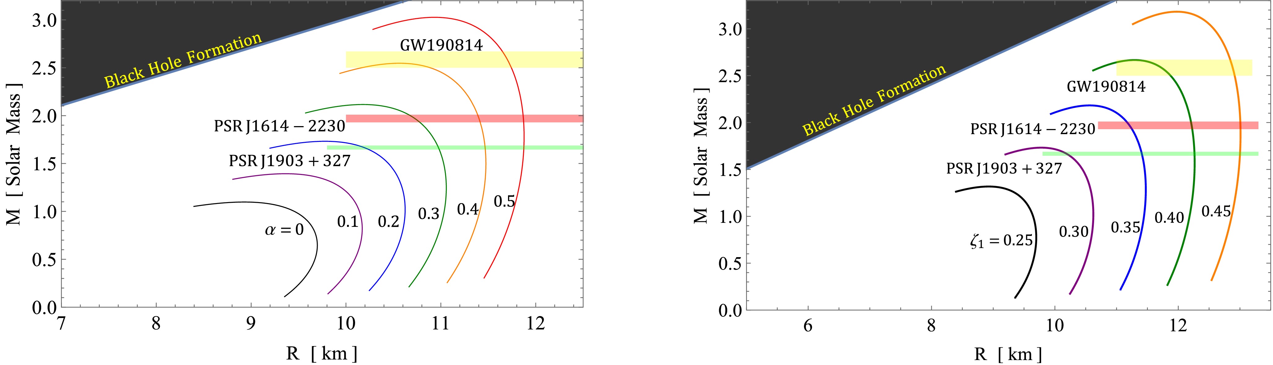

Figure 11.  (color online) The $ M-R $ curves for different free parameters values α-left panel with fixed $ \beta=0.33 $, $ \gamma=20 $, $ \zeta_1=0.3 $ and right figure shows the $ M-R $ curves for different $ \zeta_1 $ with fixed $ \alpha=0.2 $, $ \gamma=20 $, and $ \beta=0.33 $. The both figures represent the mass-radius relation for solution III B $ \left[\Theta^1_1=p_r\right] $.

Objects	$ M/M_\odot $	Predicted R [km]
		α						β
		$ 0 $	$ 0.25 $	$ 0.50 $	$ 0.75 $	$ 1.0 $		$ 0.3 $	$ 0.33 $	$ 0.36 $	$ 0.39 $	$ 0.42 $
PSR J1903+327	$ 1.667\pm 0.021 $	$ 11.61^{+0.04}_{-0.03} $	$ 11.36^{+0.04}_{-0.02} $	$ 11.15^{+0.04}_{-0.02} $	$ 10.94^{+0.02}_{-0.02} $	$ 10.74^{+0.02}_{-0.01} $		$ 11.21^{+0.03}_{-0.04} $	$ 11.18^{+0.03}_{-0.04} $	$ 11.15^{+0.03}_{-0.03} $	$ 11.13^{+0.02}_{-0.03} $	$ 11.10^{+0.03}_{-0.02} $
PSR J1614-2230	$ 1.97\pm 0.04 $	$ 12.14^{+0.04}_{-0.06} $	$ 11.87^{+0.06}_{-0.05} $	$ 11.58^{+0.05}_{-0.04} $	$ 11.28^{+0.04}_{-0.03} $	$ 10.94^{+0.02}_{-0.01} $		$ 11.66^{+0.05}_{-0.06} $	$ 11.63^{+0.05}_{-0.05} $	$ 11.60^{+0.05}_{-0.05} $	$ 11.57^{+0.04}_{-0.03} $	$ 11.54^{+0.04}_{-0.04} $
GW190814	$ 2.5-2.67 $	$ 12.96^{+0.11}_{-0.06} $	$ 12.60^{+0.11}_{-0.07} $	$ 12.17^{+0.03}_{-0.05} $	$ 11.50^{+0.03}_{-0.12} $	−		$ 12.32^{+0.08}_{-0.06} $	$ 12.26^{+0.07}_{-0.05} $	$ 12.20^{+0.06}_{-0.05} $	$ 12.13^{+0.03}_{-0.04} $	$ 12.05^{+0.01}_{-0.02} $

Table 1.  $ M-R $ curve and prediction of radii for different values of α and β for $ \rho=\Theta^0_0 $.

Objects	$ M/M_\odot $	Predicted R [km]
		γ						$ \zeta_1 $
		$ 10.0 $	$ 12.5 $	$ 15.0 $	$ 17.5 $	$ 20 $		$ 0.6 $	$ 0.7 $	$ 0.8 $	$ 0.9 $
PSR J1903+327	$ 1.667\pm 0.021 $	$ 11.20^{+0.04}_{-0.03} $	$ 11.195^{+0.04}_{-0.03} $	$ 11.19^{+0.03}_{-0.02} $	$ 11.186^{+0.02}_{-0.02} $	$ 11.18^{+0.02}_{-0.03} $		$ 9.80^{+0.02}_{-0.01} $	$ 10.40^{+0.03}_{-0.02} $	$ 10.94^{+0.03}_{-0.01} $	$ 11.46^{+0.03}_{-0.02} $
PSR J1614-2230	$ 1.97\pm 0.04 $	$ 11.67^{+0.06}_{-0.05} $	$ 11.66^{+0.06}_{-0.05} $	$ 11.64^{+0.05}_{-0.04} $	$ 11.61^{+0.05}_{-0.05} $	$ 11.59^{+0.05}_{-0.04} $		$ 10.15^{+0.04}_{-0.04} $	$ 11.78^{+0.04}_{-0.04} $	$ 11.35^{+0.06}_{-0.04} $	$ 11.90^{+0.05}_{-0.05} $
GW190814	$ 2.5-2.67 $	$ 12.35^{+0.09}_{-0.06} $	$ 12.31^{+0.08}_{-0.06} $	$ 12.27^{+0.08}_{-0.05} $	$ 12.22^{+0.05}_{-0.06} $	$ 12.16^{+0.05}_{-0.05} $		$ 10.43^{+0.02}_{-0.12} $	$ 11.17^{+0.01}_{-0.01} $	$ 11.83^{+0.02}_{-0.01} $	$ 12.44^{+0.02}_{-0.04} $

Table 2.  $ M-R $ curve and prediction of radii for different values of γ and $ \zeta_1 $ for $ \rho=\Theta^0_0 $.

Objects	$ M/M_\odot $	Predicted R [km]
		α					$ \zeta_1 $
		$ 0.2 $	$ 0.3 $	$ 0.4 $	$ 0.5 $		$ 0.25 $	$ 0.30 $	$ 0.35 $	$ 0.40 $	$ 0.45 $
PSR J1903+327	$ 1.667\pm 0.021 $	$ 10.18^{+0.06}_{-0.05} $	$ 10.97^{+0.01}_{-0.01} $	$ 11.47^{+0.01}_{-0.01} $	$ 11.88^{+0.01}_{-0.01} $		-	$ 10.20^{+0.05}_{-0.04} $	$ 11.41^{+0.01}_{-0.01} $	$ 12.26^{+0.01}_{-0.01} $	$ 13.00^{+0.01}_{-0.01} $
PSR J1614-2230	$ 1.97\pm 0.04 $	−	$ 10.73^{+0.05}_{-0.06} $	$ 11.41^{+0.01}_{-0.02} $	$ 11.87^{+0.01}_{-0.01} $		−	−	$ 11.20^{+0.05}_{-0.03} $	$ 12.21^{+0.01}_{-0.02} $	$ 13.01^{+0.01}_{-0.01} $
GW190814	$ 2.5-2.67 $	−	−	−	$ 11.71^{+0.03}_{-0.06} $		−	−	−	$ 11.75^{+0.13}_{-0.29} $	$ 12.89^{+0.03}_{-0.05} $

Table 3.  $ M-R $ curve and prediction of radii for different values of α and $ \zeta_1 $ for $ p_r=\Theta^1_1 $.

In Figures 9 and 10, corresponding to Solution III A ($ \Theta^0_0=\rho $), the $ M-R $ curves exhibit a gradual increase towards a maximum peak, followed by a sharp decrease and subsequent constancy for larger radii. This pattern highlights the variation in radius for a range of different masses of NSTRs. Remarkably, we observe that NSTRs with masses ranging from $ 2.4 $ to $ 3.5\; M_{\odot} $ correspond to a range of radii from $ 9.80^{+0.02}_{-0.01} $ to $ 13.01^{+0.01}_{-0.01}km $, determined by the values of the involved parameters α, β, γ, and $ \zeta_1 $. The intermediate part of the $ M-R $ curves indicates a smaller change in the radii. As the values of α, β, and γ increase, the peak of the $ M-R $ curves shifts downward and to the left horizontally. This suggests that higher values of α, β, and γ result in NSTRs with smaller mass and smaller radii. In contrast, as the value of $ \zeta_1 $ increases, the peak of the $ M-R $ curves shifts upward and horizontally to the right. This implies that higher values of $ \zeta_1 $ correspond to NSTRs with larger mass and larger radii. Clearly, the $ M-R $ curves associated with higher values of $ \zeta_1 $ and lower values of α, β and γ can be linked to a stiffer EOS, which supports the existence of massive NSTRs.

Moreover, in Figure 11, corresponding to Solution III B ($ \Theta^1_1=p_r $), we observe a similar trend in the $ M-R $ curves. They gradually increase towards a maximum peak, followed by a rapid decrease and subsequent constancy for larger radii. In particular, NSTRs with masses ranging from $ 2.4 $ to $ 3.5M_{\odot} $ exhibit a range of radii from $ 9.80^{+0.02}_{-0.01} $ to $ 13.01^{+0.01}_{-0.01}km $, which is determined by the values of the parameters involved α and $ \zeta_1 $. This observation supports the existence of NSTRs while excluding the variations of β and γ. We find a similar behavior for both parameters, albeit with slight differences in magnitude. As the values of α and $ \zeta_1 $ increase from $ 0 $ to $ 0.5 $ and from $ 0.25 $ to $ 0.45 $, respectively, the peak of the $ M-R $ curves shifts upward and towards the right horizontally. This indicates that higher values of α and $ \zeta_1 $ correspond to NSTRs with larger masses and larger radii. This conclusion aligns with our findings from the first solution, where higher values of α and $ \zeta_1 $ were also associated with a stiffer EOS, supporting the existence of massive NSTRs.

In earlier research work that used variational methods and EOSs for nucleonic matter, similar types of $ M-R $ curves that exhibit a significant mass around 3 $ M_\odot $ can be observed, compared to the $ M-R $ curves depicted in Figures 9, 10, and 11. An example of such research is the study conducted by [117], which investigated the scenario of the $ R^2 $ model. The findings of this study revealed that the curve $ M-R $ in the scenario of the $ R^2 $ model adheres to the general relativistic limit of approximately $ 3\; M_{\odot} $. Moreover, the upper limit of the causal mass was found to closely align with the general relativistic causal maximum mass and to fall within the region of the mass gap. Furthermore, they also delved into the concept of strange stars in the context of modified gravity, with a specific focus on the secondary component of the GW190814 event. In a separate study, [118] explored the possibility of supermassive compact stars characterized by masses ranging from approximately $ 2.2 $ to $ 2.3\; M_{\odot} $ and radii of approximately $ 11 $ km within the framework of axion $ R^2 $ gravity. In their investigation, [119] explored static NSTRs using various inflationary models commonly utilized in cosmology. Through the utilization of the MPA1 EOS, the authors found that the maximum masses of NSTRs fell within the mass gap region. In particular, these maximum masses exceeded $ 2.5\; M_{\odot} $ while still remaining below the causal limit of $ 3\; M_{\odot} $.

To determine the stability of an anisotropic neutron star in hydrostatic equilibrium, it is crucial to analyze the adiabatic index. This index plays a key role in understanding the stability characteristics of the star's configuration. In this context, [120−122] established the adiabatic stability criterion, $ \Gamma=(1+\dfrac{\rho}{p_r})(\dfrac{dp_r}{d\rho})_{{\cal{S}}} $ indicating that Γ must exceed $ 4/3 $ for stars with isotropic pressures. Here, $ \dfrac{dp_r}{dr} $ represents the speed of sound, and the subscript $ {\cal{S}} $ refers to a constant specific entropy. Herrera and colleagues found that this criterion could be modified due to anisotropy and dissipative effects such as heat flow. Consequently, the adiabatic index for a collapse scenario in an anisotropic setting is modified accordingly as [123]:

In the given expression, the term $ \dfrac{\Delta}{r|p_r|^{\prime}} $ represents the modification to the stability condition due to anisotropy where $ p_r\neq p_t $. Meanwhile, the final term $ \dfrac{r\kappa\rho p_r}{4|p_r|^{\prime}} $ accounts for the relativistic adjustment.

It has been shown that dissipative effects, such as the star's internal heat flow, can impact the adiabatic index. Consequently, a critical value for the adiabatic index ($ \Gamma_{\text{crit}} $) was proposed, dependent on two factors: (i) the compactness ($ u = \dfrac{M}{R} $) of the stellar model and (ii) a measure of the deviation from hydrostatic equilibrium (quantified by the amplitude of the Lagrangian displacement from equilibrium). The critical adiabatic parameter is expressed as $ \Gamma_{\text{crit}} = \dfrac{4}{3} + \dfrac{19}{21}u $ [124, 125]. To ensure stability against radial perturbations, Γ must be greater than $ \Gamma_{\text{crit}} $ [124]. However, it has been observed that for stable neutron stars, including white dwarfs and supermassive compact objects, Γ ranges between 2 and 4. For matter obeying a polytropic equation of state (EOS), Γ is greater than $ \dfrac{4}{3} $ and is influenced by the ratio of central density to central pressure. From Fig. (14), it is evident that our models meet the Chandrasekhar stability criterion, as the adiabatic index (Γ) increases and remains above 2 throughout the strange star models. In particular, an increase in the $ f({\cal{T}}) $ coupling constant $ \zeta_1 $ appears to make the configuration less stable. This is evident from the left panels of (Figure) for the solution $ \Theta_0^0=p_r $. However, an opposite trend can be observed for the solution $ \Theta_1^1=p_r $ in the right panel of Fig. (14). It shows that increasing the model parameter $ \zeta_1 $ results in the stability of the stellar core.

Figure 14.  (color online) Graphical analysis of adiabatic index for different values of the model parameter for the solution $ \rho=\Theta_0^0 $ and $ p_r=\Theta^1_1 $ respectively.

Furthermore, we performed a comprehensive analysis presented in a Table 4 by varying the model parameter $ \zeta_1 $ and the gravitational coupling constants α. It should be noted that increasing the MGD constant α appears to reduce the stability of the configuration for both solutions, $ \Theta_0^0=p_r $ and $ \Theta_1^1=p_r $. However, in any case, it does not violate the limit $ \Gamma>\Gamma_{\text{crit}} $.

Model-I ($ \rho=\Theta_0^0 $)		Model-II ($ p_r=\Theta_1^1 $)
$ \zeta_1 $	Γ	$ \zeta_1 $	Γ
0.2	2.224	0.2	2.031
0.4	2.104	0.4	2.049
0.6	2.065	0.4	2.055
0.8	2.058	0.8	2.057
1.0	2.056	1.0	2.059
α	Γ	α	Γ
0.05	2.276	0.05	2.415
0.10	2.038	0.10	2.279
0.15	1.845	0.15	2.149
0.20	1.694	0.20	2.031
0.25	1.567	0.25	1.935

Table 4.  Numerical values of adiabatic index for model parameter $ \zeta_1 $ and MGD constant α at the core of the stellar region.

In the previous study, Chandrasekhar introduced a method to evaluate the stability of a stellar system when exposed to radial perturbations. However, in this approach, Harrison-Zeldovich-Novikov's (HZN) stability criterion involves examining the perturbation along the physical parameters such as the metric functions, pressure, and density. Based on the HZN stability criterion [126, 127], the following constraints are established:

In this context, we analyze stability for the solution $ \rho=\Theta^0_0 $ and $ p_r=\Theta_1^1 $ in the Fig.(12) and Fig.(13) respectively. In the left panel of the graph, we present the mass profile as a function of the central density $ \rho_c $. It is evident that mass is monotonically increased while central density grows. Moreover, For a given central density of the anisotropic star, lower values of model parameter $ \zeta_1 $ lead to an increase in the total mass M of the system. Next, By varying the $ f({\cal{T}}) $ model parameter $ \zeta_1 $ for both models, we examine the rate of changes of total mass with respect to $ \rho_c $ in the right panel of Fig(12) and (13). The results show that the rate of change of mass with central density is positive and exhibits a linear trend across the entire stellar region. Therefore, the current anisotropic star model meets the stability condition.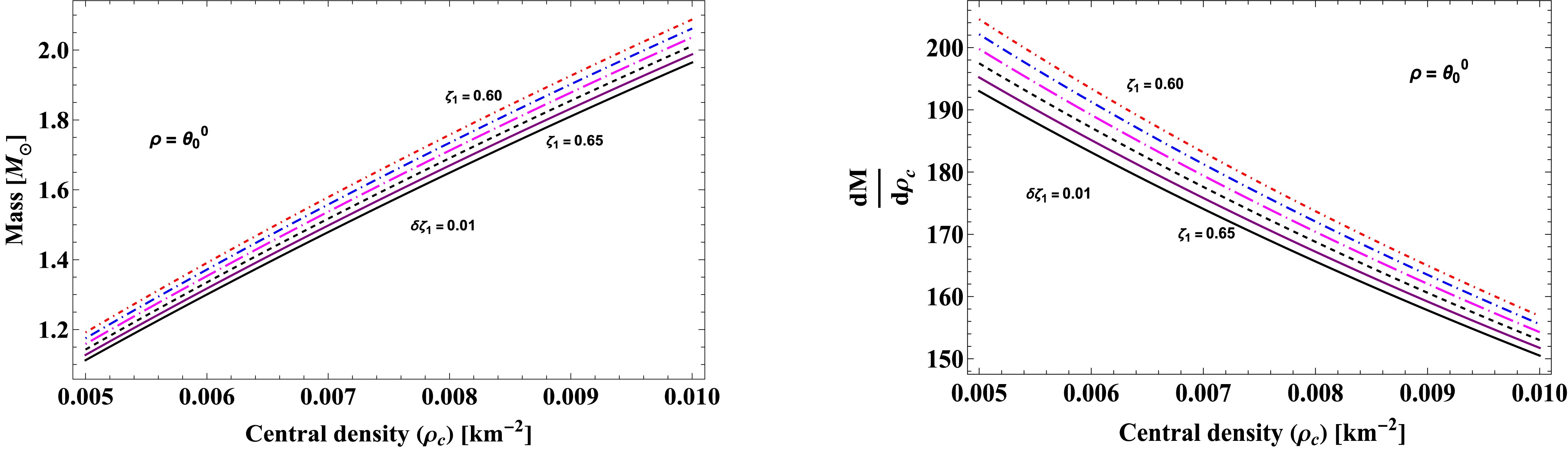

Figure 12.  (color online) Graphical analysis of mass and $ \frac{dM}{d\rho_c} $ w.r.t central density ($ \rho_c $) for different values of the model parameter for the solution $ \rho=\Theta^0_0 $.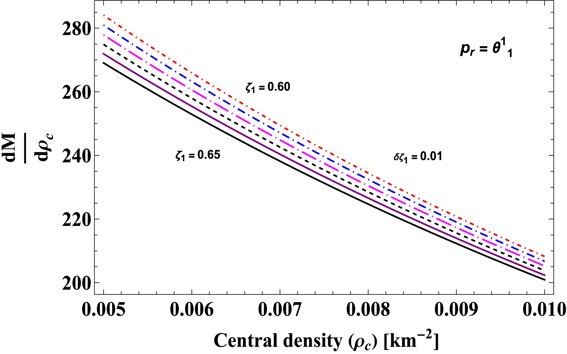

Figure 13.  (color online) Graphical analysis of mass and $ \frac{dM}{d\rho_c} $ w.r.t central density ($ \rho_c $) for different values of the model parameter for the solution $ p_r=\Theta^1_1 $.

In this section, we determine the mass of the anisotropic star using equi-mass diagrams on various planes, specifically $ B_g-\alpha $, $ B_g-\beta $, $ B_g-\gamma $, $ B_g-\zeta_1 $, and $ B_g-R $. The focus of this discussion is on the mass distribution concerning the constraints imposed by the Bag parameters $ B_g $ where $ B_g=-\frac{3\chi}{4} $. From Fig.(15), it is evident that within the range of [$ 55-90 $] $ \text{MeV}/\text{fm}^3 $, for a given $ B_g $, an increase in α corresponds to an increase in the NSTRs mass. However, there is no significant change when the MGD coupling constant α is fixed and the Bag parameter $ B_g $ is varied. This analysis strongly indicates that higher coupling constants result in more massive compact stars. Conversely, when $ \alpha\in[-1,0] $, it leads to a low-mass star, similar to a white dwarf (WD).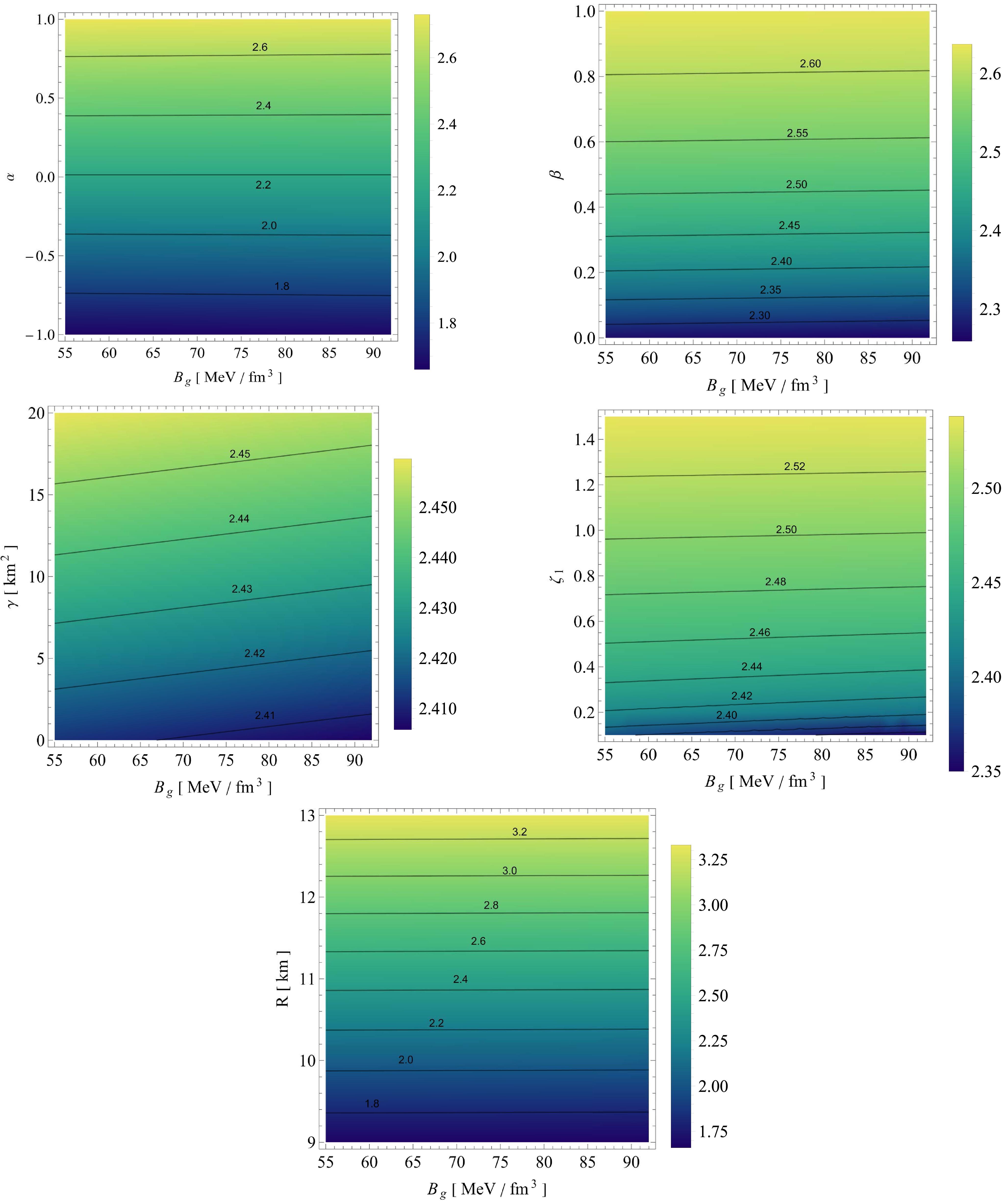

Figure 15.  (color online) The equi-mass diagram for $ B_g-\alpha $, $ B_g-\beta $, $ B_g-\gamma $, $ B_g-\zeta_1 $, and $ B_g-R $ planes where $ B_g=-\frac{3\chi}{4} $ in $ \text{MeV}/\text{fm}^3 $.

Next, we consider the $ B_g-\beta $, $ B_g-\gamma $, and $ B_g-\zeta_1 $ planes, where the mass of the NSTRs is predominantly distributed within the range of $ [2.35-2.6] $$ M_{\odot} $. It is observed that for a given $ B_g $, an increase in β, γ, or $ \zeta_1 $ results in an increase in the star's mass. However, in these three analyses, the mass exceeds the Tolman-Oppenheimer-Volkoff (TOV) limit of $ 2.1,M_{\odot} $ for a neutron star. Furthermore, no significant changes are observed when the constrained $ \gamma,\beta,\zeta_1 $ is kept constant and the Bag parameter $ B_g $ is varied.

Finally, we analyzed the $ B_g-R $ planes, observing variations in the mass distribution across a wide range of $ [1.75-3.25]M_{\odot} $. For a fixed $ B_g $, variations in the radius R result in the formation of stars ranging from low-mass WD to high-mass NSTRs. Specifically, stars with radii between 9 and 10 km correspond to low-mass stars. However, when the radius exceeds 10 km, the star surpasses the Tolman-Oppenheimer-Volkoff (TOV) limit of $ 2.1M_{\odot} $, forming massive NSTRs. In this analysis, the maximum mass observed is $ 3.25M_{\odot} $ for a radius of 13 km.

In this section, we present a concise summary of our findings in the following sequence:

1. In our recent study, we explored anisotropic stars utilizing GD through the MGD approach within the framework of $ f({\cal{T}}) $ gravity.

2. After implementing the MGD to the metric potential $ {\cal{A}}(r) $ and $ {\cal{B}}(r) $, we obtained two systems of equations, one corresponding to the seed system and the other to the Θ sector.

3. We consider a suitable polytropic EoS for the interior matter distribution of a compact star, particularly a neutron star or quark star, which reduces to the MIT bag model in the appropriate limit. Furthermore, by employing the well-established Buchdahl ansatz, we solved the seed system of equations for our constructed compact star model.

4. In the second system, the deformation function $ \psi(r) $ is obtained by the technique mimicking the physical constraints, resulting in two separate sectors: $ \rho=\Theta_0^0 $ and $ p_r=\Theta_1^1 $, each leading to distinct classes of solutions.

Following the steps outlined above, the results have been thoroughly classified and discussed in detail through various tables and figures. We have analyzed the three most critical features of the model: matter density, effective radial pressure, and effective tangential pressure. Additionally, we investigate the role of the anisotropy factor, $ \Delta^{\text{eff}} $, within the stellar sphere. It is well-established that any compact object representing the interiors of stars should be free from physical or mathematical singularities in its primary physical characteristics. The maximum values of matter density and pressure should occur at the center of the configuration and should monotonically decrease with the radial coordinate towards the surface. These novel characteristics are essential for describing real objects such as white dwarfs, NSTARS, and even quark stars. Here, we highlight some of the key features of our findings:

• From Figs. 1 and 5, it can be observed that the effective energy density consistently decreases with increasing radial distance, achieving its peak value at the core of the self-gravitating object. Importantly, these figures show that the effective energy density is regular throughout the entire interior of the configuration across all three scenarios: GR, $ f({\cal{T}}) $, and $ f({\cal{T}}) $+MGD. For the GR scenario, the core effective density is higher with $ \zeta_{1} $. In $ f({\cal{T}}) $ gravity, reducing $ \zeta{1} $ and introducing $ \zeta{2} $ decreases the core density. Conversely, in the $ f({\cal{T}}) + \text{MGD} $ model, adding α boosts the central density, concentrating matter in concentric shells. However, beyond the core, variations in α, $ \zeta{1} $, and $ \zeta{_2} $ don't affect the effective density of the star's outer layers. Apart from that, it can be observed that the effective energy density doesn't show any singularity and gives finitely bound values throughout the stellar region, indicating a viable behavior of the stellar system.

• For the $ \Theta_0^0=\rho $ solution, (III A) including (Figs. 2 and 3), we can observe that the effective radial and tangential pressures for the GR case are higher in the central region compared to the $ f({\cal{T}}) $ scenario. Additionally, in the $ f({\cal{T}}) + \text{MGD} $ scenario, the inclusion of MGD results in even lower effective radial and tangential pressures. This finding strongly indicates that MGD has a confining and compacting effect on the fluid particles, particularly in the central regions of the star. A similar pattern could be observed in the solution $ p_r=\Theta_1^1 $ (III B) in (Figs. 6 and 7). This suggests that the fluid particles are influenced by the presence of MGD, with this impact being especially noticeable in the star's central regions. Additionally, it can be observed that the radial pressure and tangential pressure remain free from singularities and maintain finite values throughout the stellar region, indicating a stable and viable behavior of the stellar system.

• Another important physical quantity is the anisotropic factor of a stellar system, which can be measured by $ \Delta^{\text{eff}}=p_t^{\text{eff}}-p_r^{\text{eff}} $. The contribution to the equilibrium of an NS/QS mechanism depends on the sign of $ \Delta^{\text{eff}} $, i.e., whether $ p_t^{\text{eff}}>p_r^{\text{eff}} $ or $ p_t^{\text{eff}}<p_r^{\text{eff}} $. We have graphically analyzed the behavior of the anisotropic factor in Figs. (4) and (8). Interestingly, the effective anisotropy, starting at zero at the star's center, gradually increases towards the outer boundary. This rise, marked by a positive $ \Delta(r) $, indicates a repulsive force from radial stresses exceeding transverse stresses. This growing anisotropy and repulsive force are key to stabilizing the star's surface layers, counteracting the inward gravitational pull, and enhancing the overall stability of the compact object. It is noteworthy that the inclusion of MGD results in a substantial increase in anisotropy within the stellar body when compared to the scenarios of GR and $ f({\cal{T}}) $. Specifically, an analysis of the GR, $ f({\cal{T}}) $, and $ f({\cal{T}}) + \text{MGD} $ scenarios reveals that the presence of MGD causes the anisotropy parameter to double. This observation underscores the significant influence of MGD on the system's anisotropic characteristics, demonstrating that MGD markedly enhances the anisotropy within the stellar body. The amplified anisotropy observed with MGD contributes to the reinforcement of the star's surface layer stability. The introduction of MGD plays a pivotal role in increasing anisotropy within the stellar fluid by creating a greater disparity between radial and tangential stresses.

• The analysis examines the impact of three relevant scenarios —- GR, $ f({\cal{T}}) $, and $ f({\cal{T}})+\text{MGD} $ — on the properties of NSTRs, using observational constraints from GW190814 with a mass range of $ 2.5-2.67M_\odot $, as well as the NSTRs PSR J1614-2230 with a mass of $ 1.97\pm 0.04M_\odot $ and PSR J1903+327 with a mass of $ 1.667\pm 0.021\; M_\odot $. The $ M-R $ curves show that NSTRs with masses ranging from $ 2.4 $ to $ 3.5M_{\odot} $ correspond to a range of radii from $ 9.80^{+0.02}_{-0.01} $ to $ 13.01^{+0.01}_{-0.01}km $, determined by the values of the parameters α, β, γ, and $ \zeta_1 $ in the two sectors, with higher values of α, β, and γ resulting in NSTRs with both smaller mass and smaller radii, and higher values of $ \zeta_1 $ corresponding to NSTRs with larger mass as well as larger radii. Clearly, the $ M-R $ curves associated with larger values of $ \zeta_1 $ for $ \rho=\Theta_0^0 $ and $ p_r=\Theta_1^1 $, and smaller values of α for $ \rho=\Theta_0^0 $ (and larger for $ p_r=\Theta_1^1 $), β, and γ can be linked to a stiffer EOS, which supports the existence of massive NSTRs within the modified $ f({\cal{T}}) $ gravity theory.

• An analysis of stability using the anisotropic generalization of the Chandrasekhar adiabatic index and the HZN stability criterion demonstrated that our models are stable. Additionally, the stability is further improved by the perturbation of the decoupling constant α and the model parameter $ \zeta_1 $.

• Finally, we determined the mass of the anisotropic star using equi-mass diagrams on various planes, specifically $ B_g-\alpha $, $ B_g-\beta $, $ B_g-\gamma $, $ B_g-\zeta_1 $, and $ B_g-R $. This discussion focuses on the mass distribution concerning the constraints imposed by the Bag parameters $ B_g $ where $ B_g=-\frac{3\chi}{4} $. It is observed from the Fig.(15) that for a given $ B_g $, an increase in α, β, γ, $ \zeta_1 $ and R results in an increase in the star's mass. However, in the analyses of $ B_g-\beta $, $ B_g-\gamma $, and $ B_g-\zeta_1 $ plane, the mass exceeds the Tolman-Oppenheimer-Volkoff (TOV) limit of $ 2.1,M_{\odot} $ for a neutron star. Additionally, no significant change is observed when the constrained $ \alpha,\gamma,\beta,\zeta_1,R $ is held constant and the Bag parameter $ B_g $ is varied. In this analysis, we obtained the maximum mass $ 3.25M_{\odot} $ in the case of $ B_g-R $ plane.

Thus, our results have provided significant insight into the complex relationship between anisotropy and the gravitational effects of $ f({\cal{T}}) $ gravity, enhancing our understanding of pulsars and their fundamental physical processes.

No new data were generated or analysed in support of this research.

SP & PKS express gratitude the National Board for Higher Mathematics (NBHM) under the Department of Atomic Energy (DAE).