Anisotropic stellar structures in the ${{f(T)}} $ theory of gravity with quintessence via embedding approach

Einstein's General Relativity (GR) has proven to be the most captivating success of the previous century. Supported by observations [1], GR enlightens several problems connected not only to the scale of the solar system but to cosmological scales as well. Numerous pieces of observational evidence from Type Ia supernovae [2, 3], the high redshifts of supernovae [4], Planck data [5], large-scale structure [6-10], and so on, indicate an accelerating expanding universe. An astonishing and contentious result from GR predicts that a matter-dominated Universe (or radiation) accelerates negatively due to the existence of gravitational attraction. The accelerated expansion of our Universe is due to dark energy (DE) [11], a mysterious galactic fluid containing a uniform density distribution, and a negative pressure, which GR cannot explain. The ambiguous behavior of DE has stimulated cosmologists to explore its apparent attributes. Modified theories of gravity are viewed as an attractive possibility to explain its nature.

DE is understood to be repulsive, exhibiting negative pressure. The equation of state $({\rm EoS})$ describing DE is $ p = \omega_q\rho $, such that $ \omega_{q}<0 $. The parameter $ \omega_q $ denotes the DE. For an expanding universe, the value of $ \omega_q $ must be restricted to $ \omega_{q}<-1/3 $. If $ \omega_q $ attains the bound $ -1<\omega_{q}<-1/3 $ then it is classified as the quintessence scalar field. In gravitational physics, quintessence is a theoretical approach for the explanation of DE. More precisely, it is a scalar field, hypothesized as a description of observing the acceleration rate of our expanding Universe. The dynamical concept of the quintessence is quite different from the explanation of DE as given by the cosmological constant in the Einstein field equations (EFEs), which is constant by definition, i.e. it does not change with time. Quintessence can behave as either attractive or repulsive, depending on the proportions of its kinetic and potential energy. It is believed that the quintessence turned repulsive around ten billion years ago, 3.5 billion years after the Big Bang. To obtain an expanding Universe, many theories have been structured but GR remains the most successful to date. In addition to its beautiful approach of enlightening diverse epochs of the Universe evolution, it has also broadened our emerging concepts of structuring gravity in the cosmos. However, there still exist some weaknesses in GR which remain unaddressed. Buchdal [12] gave the modest concept of replacing the Ricci scalar R by a function $ f(R) $ in the EFEs owing to the emergence of modified theories of gravity. Some of these are: $ f(R) $; $ f(T) $, the teleparallel theory of gravity, T being the torsion scalar; $ f(R,{\cal{T}}) $, with $ {\cal{T}} $ as the trace of the energy-momentum tensor; and $ f(G) $ and $ f(R,G) $ gravity, where G represents the Gauss-Bonnet $ ({\rm GB}) $ invariant [13-17], and has the representation $ G_{} = R^2+4R_{\mu\theta\phi\nu}R^{\mu\theta\phi\nu}-4R_{\mu\nu}R^{\mu\nu} $. These theories have enlightened the resolution of tackling the complexities involving quantum gravity and have provided researchers with various platforms through which the reasons behind the accelerating expansion of our Universe have been discussed.

The introduction of advanced experimental techniques has allowed numerous researchers to study the nature of compact stellar objects by exploring their physical attributes [18-23]. Typically, it is assumed that these stellar bodies are made up of some perfect fluid. However, recent observations confirmed that the fluid pressure of massive celestial objects such as $ 4U1820-30 $, $ PSR J 1614-2230 $, and $ SAXJ1808.4-3658(SS1) $ is not isotropic, but rather behaves anisotropically. Herrera and Santos [24] have discussed the possible existence of anisotropic fluid within the framework of self-gravitation by taking into consideration the examples of Newtonian theory and also of GR. Herrera [25] has discussed the conditions for the stability of the isotropic pressure in the framework of collapsing, spherically symmetric, dissipative fluid distributions. Capozziello et al. [26] have presented compact stellar structures possessing hydrostatic equilibrium through the Lane-Emden equation formulated for the $ f(R) $ theory of gravity. Bowers and Liang [27] have investigated locally anisotropic relativistic compact spheres through hydrostatic equilibrium and deduced that massive compact structures might be anisotropic in the presence of the fluidity-superconductivity interaction. Capozziello et al. [28], have also studied spherically symmetric solutions using the notion of Noether symmetries in the $ f(R) $ theory of gravity. Abbas et al. [29] have investigated the dynamical expressions by modeling anisotropic compact stars in the presence of the quintessence scalar field, using the Krori-Barua and Starobinsky model in the $ f(R) $ theory of gravity. Bhar [30] has structured an exclusive model for anisotropic strange stars in comparison to the Schwarzschild exterior geometry. Further, he has evaluated the EFEs by including the quintessence scalar field. From the implementation of the Krori-Barua metric he has obtained some exact solutions for compact stellar objects. Capozziello et al. [31] have worked out gravitational waves in the $ f(T,B) $ theory of gravity, produced by the corresponding compact objects. To examine a compact stellar object in the presence of the quintessence field, Kalam et al. [32] have proposed a relativistic model of compact stellar object with anisotropic pressure and normal matter. Nojiri and Odintsov [33] have established that ultimately any evolution of the Universe might be recreated for the theories under investigation. Harko and Lobo [34] have explored the possibility of mixing two different perfect fluids with different four-velocity vectors and some special parameters. Capozziello and Laurentis [35] have debated the geometrical explanation of the modified gravity theories to indicate particular suppositions in GR. It is important to point out here that $ f(T) $ gravity is simpler to understand than $ f(R) $ gravity, as its field equations are of second-order while $ f(R) $ gravity field equations are of fourth-order. However, in Refs. [36, 37] it has been argued that the Palatini version of $ f(R) $ gravity produces a system of second-order field equations. While comparing to GR, it is found [38] that $ f(T) $ gravity shows an extra degree freedom under Lorentz transformation and hence always remains non-variant. Importantly, as $ f(T) $ gravity is invariant under Lorentz transformation, the selection of good or bad tetrads plays a defining role in this particular theory. The reality of the strange stellar leftover in teleparallel $ f(T) $ gravity has been presented by Saha and his collaborators [39]. They have formulated the equation of motion by incorporating an anisotropic environment with Chaplygin gas inside. Atazadeh and Darabi [40] have explored the viable nature of $ f(R, G) $ gravity by imposing some energy conditions. Sharif and Ikram [41] have studied the warm inflation scenario in the context of Gauss-Bonnet $ f(G) $ gravity by introducing scalar fields in $ FRW $ spacetime. Maurya and Govender [42] have discussed the Einstein-Maxwell equations and presented their exact solutions for spherically symmetric stellar objects. Shamir and Zia [43] have investigated anisotropic compact structures in the $ f(R, G) $ theory of gravity. A viable approach to deriving the solutions of the field equations in the background of stellar objects has been discussed, known as the Karmarkar condition. This condition was first anticipated by Karmarkar [44], and it is considered a necessary requirement for a spherically symmetric space-time to be of embedding class I. It essentially supports us to combine the gravitational metric components. Maurya and Maharaj [45] have obtained an anisotropic embedding solution by employing a spherically symmetric geometry using the Karmarkar condition. Odintsov and Oikonomou [46] have analysed the evolving inflation and DE in the $ f(R,G) $ theory of gravity.

For the last few years, parallelism as an equivalent formulation of GR has received much consideration as an alternate gravitational theory, well acknowledged as the teleparallel equivalent of GR (TEGR) [47-49]. This formalism corresponds to the generalized manifold which takes into account a quantity known as torsion. Ferraro and Fiorini [15, 50] have investigated the TEGR modifications with consideration of cosmology, known as the $ f(T) $ theory of gravity. The fascinating part of $ f(T) $ gravity is that it gives second-order field equations, and it is structured with a generic Lagrangian quite dissimilar to the $ f(R) $ and several other theories of gravity [51, 52]. As far as theoretical or observational cosmology is concerned, numerous researchers have effectively implemented $ f(T) $ gravity in their research [38, 53-62]. Deliduman and Yapiskan [63] as well as Wang [64] have employed $ f(T) $ gravity to work out the static and spherically symmetric exact solutions describing relativistic compact objects. Deliduman and Yapiskan [65] have constructed the standard relativistic conservation equation, indicating that relativistic compact structures do not exist in the $ f(T) $ theory of gravity. However, Bohmer et al. [65] have concluded that they actually do exist. In the same line, several other investigations on $ f(T) $ gravity may be found in Refs. [66-69].

In the present study, we investigate strange compact stars in the $ f(T) $ theory of gravity with quintessence by incorporating the observational statistics of the stars $ {\rm{PSRJ1614}}-2230 $, $ 4U 1608-52 $, $ {\rm{Cen}} X-3 $, $ {\rm{EXO1785}}- 248 $, and $ SMC X-1 $. The rest of this paper is structured as follows. Section II provides the fundamental concepts of the $ f(T) $ theory of gravity. In Section III, the exclusive expressions for the physical quantities such as energy density, pressure terms, and quintessence density are worked out. Section IV is devoted to the matching conditions through the introduction of the Schwarzschild outer metric along with the comparison with the interior metric. In Section V, a detailed analysis of the physical stellar features is presented. Section VI concludes our work.

The action integral for $ f(T) $ theory is [70-72]:

where $ e = {\rm det}\left( e_{\mu}^{A}\right) = \sqrt{-g} $ and $ k^{2} = 8\pi G = 1 $. The variation of the above action results in the general form of the field equations:

where $ \overset{ e-m}{{\cal{T}}}_{i}^{\nu} $ is the energy momentum tensor, $ f_{T} $ is the derivative of $ f(T) $ w.r.t T and $ f_{TT} $ is the double derivative w.r.t T, $ \overset{ e-m}{{\cal{T}}}_{i}^{\nu} = \overset{ matter}{{\cal{T}}}_{i}^{\nu}+\overset{ q}{{\cal{T}}}_{i}^{\nu} $, and $ \overset{ q}{{\cal{T}}}_{i}^{\nu} $ is the energy-momentum for the quintessence field equations with energy density $ \rho_{q} $ and equation of state parameter $ w_{q} $$\left( -1<w_{q}<-\dfrac{1}{3} \right)$. Here the components of $ \overset{ q}{{\cal{T}}}_{i}^{\nu} $ are defined as:

The torsion and the super-potential tensors used in Eq. (2) are given in general as:

The density of the teleparallel Lagrangian is defined by the torsion scalar as

For the present investigation, the character of the scalar torsion T is of crucial importance.

Due to the flatness of the manifold, the Riemann curvature tensor turns out to be zero. Containing the two fragments, one part of the curvature tensor defines the Levi-Civita connection, while the second part provides the Weitzenböck connection. Similarly, the Ricci scalar R also delivers two dissimilar geometrical entities. Keeping this in view, the torsion-less Ricci scalar R in the Einstein- Hilbert action, in the shape of the torsion, which may be viewed as an expression of T, as given above, can be reproduced. It should be noted that the teleparallel theory of gravity has been found similar to GR under the two separate contexts of local Lorentz transformation and arbitrary transformation coordinates. The first part is non-trivial to observe, and the second Lorentz part adequately delivers the geometry in such way that the construction of the teleparallel action of the GR fluctuates from its metric formulation because of its surface expression. Likewise, one can envision that the modified $ f(R) $ and $ f(T) $ theories of gravity display a resemblance to their surface geometries, which are due to the local Lorentz invariance, affected by the $ f(R) $ theory of gravity.

Here we build stellar structures by taking the spherically symmetric spacetime

where $ a(r) $ and $ b(r) $ solely depend on the radial coordinate r. We will deal with these metric potentials using the Karmarkar condition in the later part of this work. Nicola and Bohmer [73] have shown some reservations by declaring the diagonal tetrad to be an incorrect choice in torsion based theories of gravity, as this bad tetrad raises certain solar system limitations. They have also mentioned in their study that a good tetrad has no restrictions on the choice of the model of $ f(T) $ being linear or non-linear, while the diagonal tetrad restricts the $ f(T) $ model to a linear one. The off-diagonal tetrad is a correct choice due to its boosted and rotated behavior [38]. Here we calibrate the field equations by using the off-diagonal tetrad matrix:

Here e is the determinant of $ e_{\mu}^{\nu} $, given as $ {\rm e}^{a(r)+b(r)}r^{2} \sin\theta $. The energy momentum tensor for an anisotropic fluid defining the interior of a compact star is

where $ u_{\gamma} = {\rm e}^{\frac{\mu}{2}}\delta_{\gamma}^{0} $, $ v_{\gamma} = {\rm e}^{\frac{\nu}{2}}\delta_{\gamma}^{1} $, and $ \rho $, $ P_{r} $ and $ P_{t} $ are the energy density, radial pressure and tangential pressure respectively.

Manipulating Eqs. (2)-(11), we have the following important expressions:

In the above equations F is the derivative of f with respect to the torsion scalar $ T(r) $, and the prime on F again is the derivative of F with respect to $ T(r) $. The torsion $ T(r) $ and its derivative with respect to the radial coordinate r are given as:

The diagonal tetrad provides the linear algebraic form of the $ f(T) $ function. The off-diagonal tetrad, however, does not result in any parameter which restricts the construction of a consistent model in $ f(T) $ gravity. The following extended teleparallel $ f(T) $ power law viable model [74] is given as:

where $ \beta $, and k are any real constants. For the power-law model, if we put $ k = 1 $, we get teleparallel gravity. If we put $ k>1 $, we get generalized teleparallel gravity. In this study, we take $ k = 2 $, which is a well fitted value with the off-diagonal tetrad choice. For $ f(T) $ gravity, the underlying scenario gives realistic solutions for stellar objects with normal matter except in a particular range of radial coordinates with observed data.

Now we discuss the Karmarkar condition, which is an integral tool for the current study. The groundwork with regard to the Karmarkar condition has been established for class-I space-time. Eisenhart [75] provided a sufficient condition for the symmetric tensor of rank two as well as the Riemann Christoffel tensor, and it is defined as

Here, ";" stands for the covariant derivative and $ \Sigma = \pm1 $. These values signify a space-like or time-like manifold, depending whether the sign is $ - $ or $ + $. Now, by taking into account Riemann curvature components, which are non-zero for the geometry of the space-time and by also conferring non-zero components of the symmetric tensor $ \Lambda_{\nu\eta} $, which is of order two, we incorporate a relation as follows. Now the relation for the Karmarkar condition is defined as:

and we have the following Riemannian non-zero components:

Fitting the above values of the Riemannian components in Eq. (16) gives rise to a differential equation having form

Embedding class one solutions are obtained from Eq. (18), as they can be embedded in 5-dimensional Euclidean space. By the integration of Eq. (18), we have

or exclusively

where A and B are the integration constants. The final expressions for energy density and pressure components are calculated as:

where

No matter what remains of the geometrical structure of the star, whether exterior or from the interior, the inner boundary metric does not change. This requires that the metric components remain continuous along the entire boundary. In GR, the Schwarzschild solution associated with the stellar remnants is understood to be the top choice from all the available options for the matching conditions. Any suitable choice when working with theories of modified gravity must consider the non-zero pressure and the energy density. Several researchers [76-77] have produced significant work on the boundary conditions. Goswami et al. [78] worked out the matching conditions while investigating modified gravity by incorporating some special limitations to stellar compact structures along with the thermodynamically associated properties. Many researchers [79-82] have effectively employed Schwarzschild geometry while working out the diverse stellar solutions. To obtain the expressions for the field equations, a few restrictions are applied at the boundary $ r = R $, that is $ p_r(r = R) = 0 $. Here, we also intend to match the Schwarzschild exterior geometry with the interior geometry:

where M represents the total stellar mass and R is the total radius of the star. Taking into account the metric potentials, the following relations are employed at the boundary $ r = R $:

The signatures of the intrinsic geometry and extrinsic geometry are taken as (-,+,+,+) and (+,-,-,-), respectively. The desired restrictions are achieved by comparing the interior and exterior geometry as they are, and working out the following:

The approximate values of the mass M and the radius R of the stellar objects $ {\rm{PSRJ1614}}-2230 $, $ 4U 1608-52 $, $ {\rm{Cen}} X-3 $, $ {\rm{EXO1785}}-248 $, and $ SMC X-1 $ are considered to determine the unknowns as given in Table 1.

Star name	Observed mass ($M_{o}$)	Predicted radius ($R km$)	a	A	B
PSRJ1614-2230	1.97	12.182	0.0023099	0.734147	0.0233421
4U 1608-52	1.74	11.751	0.00228432	0.758428	0.0231551
CenX-3	1.49	11.224	0.00225723	0.785203	0.0229539
EXO1785-248	1.3	10.775	0.00223401	0.80602	0.0227945
SMCX-1	1.04	10.067	0.00219944	0.835374	0.0225762

Table 1.  Values of constants of compact stars by fixing $ k=2 $, $b=0.000015,$ $\gamma =0.333$, $w_q=-1.00009$, $c=0.000015$ and $\beta =-4$.

This section is dedicated to the exploration of some critical properties connected to the compact stars. These comprise the energy density $ \rho $, radial pressure $ p_r $, the tangential pressure $ p_t $, and the discussions on the quintessence field along with their physical interpretation under $ f(T) $. This discussion also includes the energy conditions, anisotropic pressure, compactness factor, and the speed of sound in the star with reference to the radial and tangential components. The smooth and regular behavior of the metric components is plotted in Fig. 1.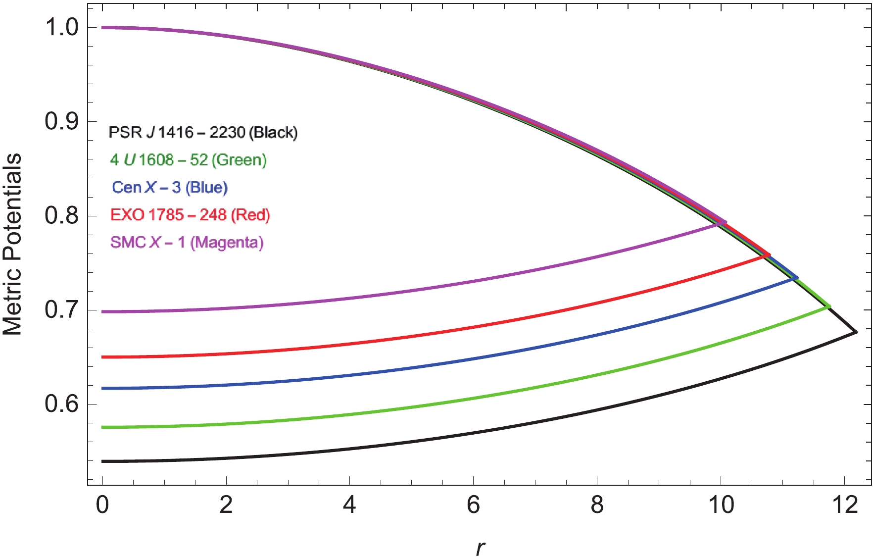

Figure 1.  (color online) Evolution of metric potentials versus r. Here we fix $ k=2 $, $b=0.000015$ $\gamma =0.333$, $w_q=-1.00009$, $c=0.000015$ and $\beta =-4$.

The most important stellar environment responsible for the emergence of the compact stars comprises the corresponding profiles of the energy density along with the radial and tangential pressures. We have investigated the profiles of the energy density, quintessence density and pressure terms. It is apparent from the plots, as shown in Figs. 2 and 3, that the energy density acquires its highest value at the center of the star, indicating the ultra-dense nature of the star. The tangential and radial pressure terms are positive and acquire their maximum values at the surface of the compact stars. The profiles of the stars also indicate the presence of an anisotropic matter configuration free from any singularities for our model under $ f(T) $ gravity.

Figure 2.  (color online) Evolution of energy density $\rho$ (left) and quintessence density $\rho_q$ (right).

Figure 3.  (color online) Evolution of radial pressure $p_r$ (left) and tangential pressure $p_t$ (right).

The role of the energy constraints, among the other physical features in describing the existence of anisotropic compact stars, has been widely acknowledged in the literature, as they allow analysis of the environment to obtain the matter distribution. Moreover, the energy constraints also allow analysis of the distribution of normal and exotic matter contained within the core of the stellar structure. Several fruitful conclusions have been obtained due to these energy constraints. The expressions corresponding to the null energy constraints $ ({\rm NEC}) $, strong energy constraints $ ({\rm SEC}) $, dominant energy constraints $ ({\rm DEC}) $, and weak energy constraints $ ({\rm WEC}) $ are:

The evolutions of the energy constraints are plotted in Fig. 4. It is clear from the positive profiles of the energy conditions for all the stars, $ {\rm{PSRJ1614}}-2230 $, $ 4U 1608-52 $, $ {\rm{Cen}} X-3 $, $ {\rm{EXO1785}}- 248 $, and $ SMC X-1 $, that our obtained solutions are physically favorable under $ f(T) $ gravity.

Figure 4.  (color online) Evolution of energy conditions (left) and forces (right).

The expressions $\dfrac{{\rm d}\rho}{{\rm d}r}$, $\dfrac{{\rm d}p_{r}}{{\rm d}r}$ and $\dfrac{{\rm d}p_{t}}{{\rm d}r}$ denote the total derivatives of the energy density, the radial pressure, and the tangential pressure, respectively, with respect to the radius r of the compact star. The graphical description of these radial derivatives is provided in the right-hand plots of Fig. 5, which suggest that the first order derivative gives a negatively increasing evolution: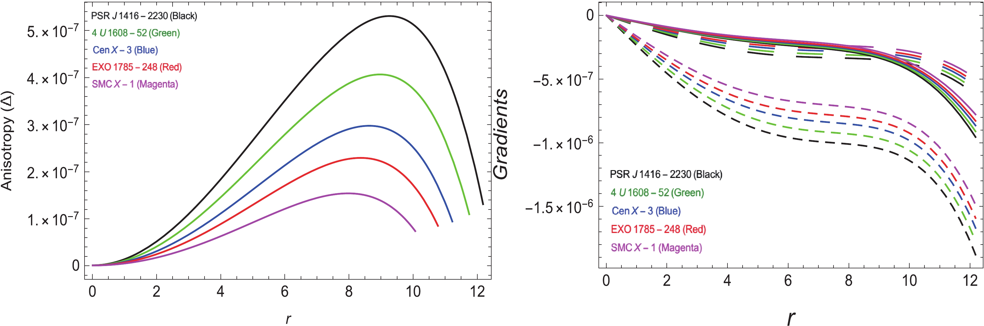

Figure 5.  (color online) Evolution of anisotropy $\Delta$ (left) and gradients (right).

It may be noted that $\dfrac{{\rm d}\rho}{{\rm d}r}$ and $\dfrac{{\rm d}p_{r}}{{\rm d}r}$ at the core, $ r = 0 $, of the star are:

This confirms the maximum bound of the radial pressure $ p_r $ along with the central density $ \rho $. Hence, the maximal value is attained at $ r = 0 $ by $ \rho $ and $ p_r $.

The generalized TOV equation in anisotropic matter distribution is given as

where Eq. (32) provides important information about the stellar hydrostatic-equilibrium under the total effect of three different forces, namely the anisotropic force $ F_{\rm a} $, the hydrostatic force $ F_{\rm h} $, and the gravitational force $ F_{\rm g} $. The null effect of the combined forces depicts the equilibrium condition such that

with

From the right plot-hand of Fig. 4, it may be deduced that under the combined effect of the forces $ F_{\rm g} $, $ F_{\rm h} $ and $ F_{\rm a} $, hydrostatic compact equilibrium can be achieved. It is pertinent to mention here that if $ p_{r} = p_{t} $ then the force $ F_{\rm a} $ vanishes, which simply conveys that the equilibrium turns independent of the anisotropic force $ F_{\rm a} $.

The stability is constituted by the speed of sound associated with the radial and transverse components, denoted $ v^{2}_{sr} $ and $ v^{2}_{st} $, respectively. They must satisfy the constraints $ 0\leqslant{v^{2}_{st}}\leqslant 1 $ and $0\leqslant{v^{2}_{sr}}\leqslant1$ [83], such that $= v^{2}_{sr} = \dfrac{{\rm d}p_{r}}{{\rm d}\rho}$ and $v^{2}_{st} = \dfrac{{\rm d}p_{t}}{{\rm d}\rho}$. A comprehensive study of the stability of anisotropic spheres has been done by Chan and his coauthors [84]. They have discussed Newtonian and post-Newtonian approximations in the background of anisotropy distribution. The corresponding plots of the speeds of sound as depicted in Fig. 6 confirm that the evolution of the radial and transverse speed of sound for the strange star candidates $ {\rm{PSRJ1614}}-2230 $, $ 4U 1608-52 $, $ {\rm{Cen}} X-3 $, $ {\rm{EXO1785}}-248 $, and $ SMC X-1 $ remain within the desired constraints of stability as discussed. For all the strange star candidates the bounds of both the radial and the transverse speeds of sound are justified. Within the anisotropic matter distribution, the approximation of the theoretically stable and unstable epochs may be obtained from the modifications of the propagation of the speed of sound, which has the expression $ v^{2}_{st}-v^{2}_{sr} $ satisfying the constraint $ 0<|v^{2}_{st}-v^{2}_{sr}|<1 $. One may confirm this from Fig. 7. Therefore, the total stability may be obtained for compact stars modelled under $ f(T) $ gravity.

Figure 6.  (color online) Evolution of EoS $w_t$.

Figure 7.  (color online) Evolution of speeds of sound $v_{r}^{2}$ (left) and $v_{t}^{2}$ (right).

For the case of anisotropic matter distribution, the EoS parameter incorporating radial and transverse components may be expressed as

The analysis of the EoS parameters with respect to the increasing stellar radius is graphically represented in Fig. 8 which clearly demonstrates that for all strange star candidates $ {\rm{PSRJ1614}}-2230 $, $ 4U 1608-52 $, $ {\rm{Cen}} X-3 $, $ {\rm{EXO1785}}-248 $, and $ SMC X-1 $, the conditions $ 0<\omega_{r}<1 $ and $ 0<\omega_{t}<1 $ have been obtained. Hence, our stellar model in $ f(T) $ gravity is truly viable. Now, the anisotropy here is expressed by the symbol $ \Delta $, and is measured as

Figure 8.  (color online) Evolution of $\mid v_{r}^{2}$-$v_{t}^{2}\mid$.

which provides the information regarding the anisotropic conduct of the model under discussion. The term $ \Delta $ has to be positive if $ p_t>p_r $, showing that the anisotropy is going outward, and when $ p_r>p_t $, $ \Delta $ becomes negative, showing that it will be directed inward. For our model incorporating all the stars $ {\rm{PSRJ1614}}-2230 $, $ 4U 1608-52 $, $ {\rm{Cen}} X-3 $, $ {\rm{EXO1785}}-248 $, and $ SMC X-1 $, the evolution of $ \Delta $ when plotted against radius r shows positive increasing behavior (as shown in the left-hand plot of Fig. 5), suggesting some repelling anisotropic force followed by a high-density matter source.

The stellar mass as a function of radius r is defined by the following integral:

It is evident from the mass-radius graph as shown in Fig. 9 that the mass is directly proportional to the radius r such that as $ r\rightarrow0 $, $ m(r)\rightarrow0 $, showing that mass function remains continuous at the core of the star. Also, the mass-radius ratio must remain $\dfrac{2M}{r}\leqslant\dfrac{8}{9}$ as determined by Buchdahl [85], which in our case is within the desired range.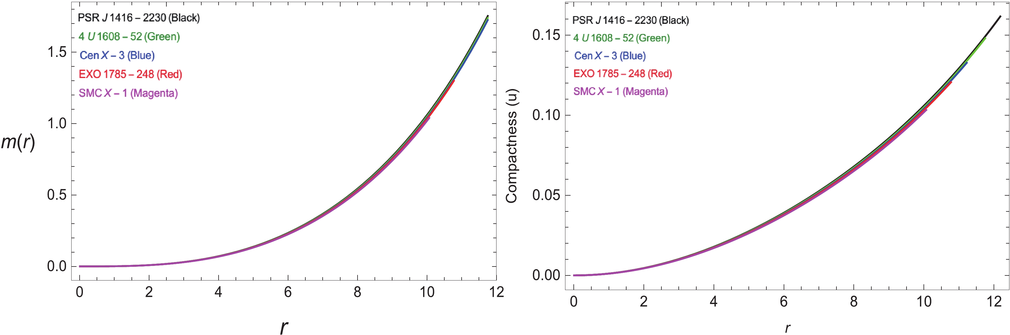

Figure 9.  (color online) Evolution of mass function (left) and compactness parameter (right).

Now, the following integral defines the compactness $ \mu(r) $ (plotted in Fig. 9) of the stellar structure as

The redshift function $ Z_{S} $ is

The graphical representation is provided in Fig. 10. The numerical estimate of $ Z_{S} $ remains within the desired condition of $ Z_{S}\leqslant 2 $, indicating the viability of our model.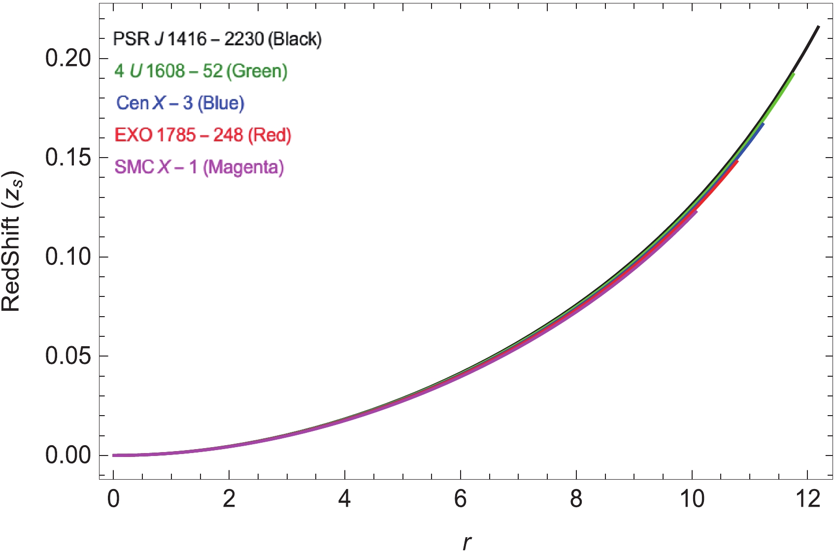

Figure 10.  (color online) Evolution of redshift function.

As an equivalent structuring of GR, the notion of parallelism has been raised in the last few years as an attractive alternate theory of gravity, and has been well acknowledged as the teleparallel equivalent of GR (TEGR). The concept behind this is the existence of an even more standard manifold which takes into account the curvature, besides a quantity called torsion. A large number of scholars have explored the modifications of TEGR with reference to cosmology, the $ f(T) $ theory of gravity. The most attractive aspects of $ f(T) $ gravity is that it has second-order field equations dissimilar to those of $ f(R) $ gravity, and it is built with a comprehensive Lagrangian.

In our present work, we have employed a general model for the possible existence of static and anisotropic compact structures in the spherically symmetric metric and by using a power law model in the framework of $ f(T) $-modified gravity. To the best of our knowledge, this is the first attempt to study stellar objects in the $ f(T) $ theory of gravity with quintessence via an embedding approach. Our theoretical calculations support realistic models of the stars $ {\rm{PSRJ1614}}-2230 $, $ 4U 1608-52 $, $ {\rm{Cen}} X-3 $, $ {\rm{EXO 1785}}-248 $, and $ SMC X-1 $. The stability and singularity-free nature of these realistic models is physically important, and our results are in good agreement in this scenario. Moreover, through some manipulations, the corresponding field equations are solved for the compact stars. We have established our calculations under the assumptions of the statistics corresponding to the $ {\rm{PSRJ1614}}-2230 $, $ 4U 1608-52 $, $ {\rm{Cen}} X-3 $, $ {\rm{EXO1785}}- $ 248, and $ SMC X-1 $, as strange star candidates with appropriate choice of the values of the parameter n. Our work here applies the investigation of the possible existence of quintessence to compact stars with an anisotropic nature due to the extremely dense structure in the framework of the $ f(T) $ theory of gravity. For the evolving Universe in different epochs, gravitational stellar collapse has been explored by incorporating the spacetime symmetries along with exclusive matching of the Schwarzschild vacuum solution. Graphical illustrations of some exclusive features of the quintessence stellar structures in $ f(T) $ gravity have been presented. The energy density $ \rho $, the transverse pressure $ p_t $, the radial pressure $ p_r $, anisotropy limitations and the quintessence energy density $ \rho_q $ have been analysed in the context of $ f(T) $ gravity by using the off-diagonal tetrad and power law given as $ f(T) = \beta T^n $. Here are some of the key features which we have found during our investigation, with our focus on the energy density, radial and tangential pressures and the quintessence field, along with their physical interpretation under $ f(T) $ gravity. Other interesting features include the energy restrictions, anisotropy, compactness and the speed of sound of the stellar remnants in terms of both radial and tangential components.

● The crucial physical aspects for the existence of stellar structures comprise the energy density and the radial and tangential pressures. It is clear from the respective plots in Figs. 2 and 3 that the energy density at the stellar core attains the highest value, showing the highly dense character of the star. Also, the tangential and radial pressure terms are positive and attain their maximum values at the star surface. These profiles also offer the existence of anisotropic matter distribution independent of singularities for the $ f(T) $ model under investigation. Furthermore, the profiles of the quintessence density $ \rho_q $ show negative behavior, favoring our stellar $ f(T) $ gravity model.

● The role of the energy constraints is quite obvious in the literature on compact stellar remnants. The plots of the corresponding energy conditions have been presented in Fig. 4. It is evident from the positive profiles for all the stars, $ {\rm{PSRJ1614}}-2230 $, $ 4U 1608-52 $, $ {\rm{Cen}} X-3 $, $ {\rm{EXO1785}}-248 $, and $ SMC X-1 $, that our acquired solutions are physically viable in $ f(T) $ gravity.

● The profiles of $\dfrac{{\rm d}\rho}{{\rm d}r}$, $\dfrac{{\rm d}p_{r}}{{\rm d}r}$ and $\dfrac{{\rm d}p_{t}}{{\rm d}r}$, the total derivatives of $ \rho $, $ p_r $, and $ p_t $ with respect to the stellar radius r, respectively, have been provided in Fig. 5. This indicates that the first derivative shows negatively accelerating evolution. This validates the highest bound of the radial pressure $ p_r $ with the central density $ \rho $. Therefore, the highest value is achieved by $ \rho $ and $ p_r $ at $ r = 0 $.

● For the hydrostatic equilibrium, it is evident from the right-hand panel of Fig. 4 that under the total effect of the forces $ F_{\rm g} $, $ F_{\rm h} $ and $ F_{\rm a} $, stellar equilibrium is achieved. It is worth mentioning that in certain situation like $ p_{r} = p_{t} $, the force $ F_{\rm a} $ vanishes, hinting that the equilibrium is free of the effect of anisotropic force $ F_{\rm a} $.

● The corresponding plots of the speeds of sound, shown in Fig. 6, suggest that the radial and transverse speeds of sound for all the stars, $ {\rm{PSRJ1614}}-2230 $, $ 4U 1608-52 $, $ {\rm{Cen}} X-3 $, $ {\rm{EXO1785}}-248 $, and $ SMC X-1 $, are bounded within the desired constraints of stability. One may confirm from Fig. 7 that the constraint $ 0<|v^{2}_{st}-v^{2}_{sr}|<1 $ for the stability of the compact star is achieved. Therefore, overall stability may be obtained for compact stars modeled under $ f(T) $ gravity.

● The constraint parameter EoS is expressed by $ 0<\omega_{t}<1 $ and is plotted in Fig. 8. It is easy to see that it favors the corresponding matter distribution under $ f(T) $ gravity.

● For the stars $ {\rm{PSRJ1614}}-2230 $, $ 4U 1608-52 $, $ {\rm{Cen}} X-3 $, $ {\rm{EXO1785}}-248 $, and $ SMC X-1 $, the anisotropy $ \Delta $ with respect to r gives positive increasing behavior (as shown in the left-hand plot of Fig. 5), suggesting repelling anisotropic forces incorporated by a high-density matter source.

● Figure 10 provides graphical representation of the red-shift function. The approximate value of $ Z_{S} $ falls within the desired condition of $ Z_{S}\leqslant 2 $, supporting our model.

It is worth mentioning here that the solutions we have obtained in this study represent denser stellar structures than those in past related works on compact objects in extended theories of gravity [29, 86-88].

We are grateful to the anonymous referees for their valuable comments, which improved the presentation of this paper.