Copositive criteria for a two-component dark matter model

The Standard Model (SM) of particle physics has been remarkably successful in describing fundamental particles and their interactions. However, astrophysical observations indicate the existence of dark matter (DM), which constitutes approximately $ 26.5 $% of the mass-energy content of the universe [1]. The existence of DM can be inferred from its gravitational effects on the large-scale structure of the universe; however, its particle nature remains elusive. In terms of particle physics, dark matter (DM) can be assumed to be some stable particles that carry no SM gauge group quantum number.

Weakly interacting massive particles (WIMPs) are one of the most popular and attractive DM candidates [2−4], wherein the observed DM relic density is generated via the ''Freeze-out'' mechanism [5]. Among the different WIMP models, the singlet scalar DM model is the simplest one, wherein a new singlet scalar as DM is introduced to the SM. The singlet scalar is stabilized by extra $ Z_2 $symmetry, and there are only two free model parameters in the model with a DM mass and quartic coupling of DM with SM Higgs. The viable DM mass region is restricted by the Higgs invisible decay search at the LHC [6], DM relic density, direct detection constraint [7, 8], and indirect detection constraint attributed to the gamma-ray spectrum induced by DM annihilation observed at Fermi-LAT [9, 10] and HESS [11]. This causes the resonant mass to be approximately half of the SM Higgs mass and high mass region to be larger than approximately 3 TeV [12]. Current direct detection experiments do not yield a clear signal, which imposes stringent constraints on DM-nucleon interactions and present a significant challenge for WIMP scenarios.

A possible solution to the problem is a multi-component DM model, which includes two or more DM species. In this model, one of the DM candidates has a large elastic cross-section on the nuclei; however, it forms a subdominant DM component that leads to a suppressed signal [13], causing it to escape the direct detection constraint. In addition, there is no preference to assume that there is only one DM candidate in the universe, and discussions about multi-component DM have been previously reported [14−17]. For a multi-component scalar DM model, an extra symmetry such as $ Z_2 \times Z_2' $ [18], $ Z_5 $ symmetry [19−21], $ Z_7 $ symmetry [22], or other $ Z_N $ symmetry [23−25] can be considered to ensure the stability of DM particles.

When constructing a viable multi-component scalar DM model, the stability of the electroweak vacuum needs to be guaranteed. Scalar field theories suggest that the concept of vacuum stability is intricately linked to the properties of the scalar potential, particularly, its quartic couplings. A scalar potential bounded from below is a prerequisite for stable vacuum, which leads to copositive criteria. Copositive matrices are a class of matrices that are positive on non-negative vectors and provide a mathematical framework to assess the stability conditions of scalar potentials. These matrices enable deriving the necessary and sufficient analysis conditions for vacuum stability, which is essential for ensuring that the scalar potential does not lead to unphysical situations such as a vacuum that is not the global minimum of the potential.

Discussion about copositive criteria and DM have been presented in [26−31]. In this study, we consider a simple two-component scalar DM model and discuss the copositive criteria for the model. We introduce three singlet scalars $ S_1 $, $ S_2 $, and $ S_3 $ to the SM, where $ S_1 $ and $ S_2 $ represent DM candidates and $ S_3 $ has a non-zero vacuum expectation value. We obtain the two component scalar DM model [17] when $ S_3 $ is absent, which necessitates a large $ \lambda_{12} $ to evade direct detection and relic abundance constraints outside the Higgs resonance region. The introduction of$ S_3 $ leads to new annihilation channels and couplings of DM with SM Higgs. $ \lambda_{12} $ can be smaller to escape the direct detection constraints with the observed DM relic density constraint. The existence of $ S_3 $ contributes to the new DM annihilation processes so that a wider parameter space compared to those of DM models that involve only two singlet scalars can be obtained. A $ 4\times 4 $ copositive matrix of quartic couplings can be constructed in the model. The copositive criteria of a rank $ \leqslant 3 $ matrix can be obtained concretely, whereas for a matrix with a higher rank, related discussions about the models are ignored becuase of their complexity. In this study, we analyze the copositive criteria of the model systematically. We consider eight cases of the copositive criteria for a rank 4 matrix; more complex cases can be obtained when considering the signs of the model couplings. Based on the direct detection constraint, we consider four different cases from the point of exchange symmetry for simplicity and estimate the viable parameter space within the DM relic density and direct detection constraints. The signs of the couplings can not only determine the copositive criteria but also make a difference in the cross-section of $ 2 \to 2 $ processes related to DM annihilation into other scalars attributed to the interference effect. We randomly scan the selected parameter space and focus on quartic couplings with $ \lambda_{13} $, $ \lambda_{23} $, $ \lambda_{14} $, and $ \lambda_{24} $. The allowed values of $ (|\lambda_{13}|,|\lambda_{14}|) $ are different for all four cases; however, all of them require the new Higgs to play a dominant role in determining DM relic density. Within the viable parameter space, copositive criteria place stringent constraints as long as some coupling is negative.

The rest of this manuscript is organized as follows. We present a two-component scalar DM model in Sec. II. In Sec. III, we discuss the copositivity of the symmetric matrix with eight different cases. In Sec. IV, we consider the DM phenomenology of the model including relic density and direct detection. In Sec.V, we consider four different cases by fixing some of the quartic parameters to be negative and discuss the effect of copositive constraint on a viable parameter space satisfying the relic density and direct detection constraints. Finally, we present a summary in Sec. VI.

We establish a simple two-component scalar DM model with $ Z_2 \times Z_2' \times Z_2'' $ symmetry by introducing three singlet scalars $ S_{1,2,3} $ into an SM model. The corresponding charges for DM particles $ S_1 $ and $ S_2 $ are $ (-1,1,1) $ and $ (1,-1,1) $, and $ S_3 $ has a non-zero vacuum expectation value (vev) carrying the $ (1,1,-1) $ charge, while the SM particles carry a $ (1,1,1) $ charge. Therefore, the potential part of the scalars can be given by

where H represents the SM Higgs doublet. The $ Z_2'' $ symmetry is introduced to simplify the scalar potential in this study. Under unitarity gauge, H and $ S_3 $ can be expressed as

where $ v_0 = 246 $ GeV corresponds to the electroweak symmetry breaking vev and $ v_1 $ represents the vev of $ S_3 $. After spontaneous symmetry breaking (SSB), the masses of $ S_1 $ and $ S_2 $ can be given by

where $ m_1(m_2) $ represents the mass of $ S_1(S_2) $. We have the squared mass matrix of $ s_3 $ and h with

The physical masses of the two Higgs states $ h_1, h_2 $ are

The mass eigenstate ($ h_1,h_2) $ and gauge eigenstate ($ h, s_3 $) can be related as

where

Furthermore, we can assume that $ h_1 $ represents the observed SM Higgs and $ h_2 $ represents the new Higgs in our model. The masses of the Higgs particles $ m_{h_1} $ and $ m_{h_2} $ can be selected as inputs, and the couplings of $ \lambda_H $, $ \lambda_{33} $, and $ \lambda_{34} $ can be given by

The extended scalar field models beyond the SM can contain complicated quartic couplings, and therefore, it is important to formulate criteria that define the boundedness of the potential with the largest parameter space in terms of the vacuum stability constraint. One possible idea is constructing the quartic couplings as a pure square of the combinations of bilinear scalar fields and setting their coefficients to be non-negative. We imported the idea of copositivity of symmetric matrices in this study. In our model, the scalar potential quartic terms can be given with a symmetric matrix as

In the following discussion, we use $ \lambda_{44} $ to represent $ \lambda_H $ for the sake of coherence. For this symmetric matrix of order four, we use eight different cases based on the sign distributions of off-diagonal elements to determine if this matrix is copositive. In these cases, all diagonal elements need to be positive as a generic condition. The eight cases are presented below [28].

● Case I: Matrix $ {\cal{S}} $ is copositive if and only if $ \lambda_{ii} \geq 0 $ when all off-diagonal elements are positive.

● Case II: Matrix $ {\cal{S}} $ is copositive if and only if $ (\lambda_{ii}\lambda_{jj}-\lambda_{ij}^2) \geq 0 $ when $ \lambda_{ij} \leq 0 $ and other off-diagonal elements are positive.

● Case III: Matrix $ {\cal{S}} $ is copositive if and only if $ (\lambda_{ii}\lambda_{jj}-\lambda_{ij}^2)\geq 0, (\lambda_{ll}\lambda_{kk}-\lambda_{lk}^2) \geq 0 $ when $ \lambda_{ij},\lambda_{lk} \leq 0 $ and other off-diagonal elements are positive.

● Case IV: When $ \lambda_{ij},\lambda_{ik} \leq 0 $, we need $ (\lambda_{ii}\lambda_{jk}-\lambda_{ij}\lambda_{ik}+ \sqrt{(\lambda_{ii}\lambda_{jj}-\lambda_{ij}^2)(\lambda_{ii}\lambda_{kk}-\lambda_{ik}^2)}) \geq 0 $ to ensure that matrix $ {\cal{S}} $ is copositive.

● Case V: Matrix $ {\cal{S}} $ is copositive if and only if the following order three matrix is copositive:

when $ \lambda_{ij},\lambda_{jk},\lambda_{ik}\leq 0 $ and the other off-diagonal elements are positive.

● Case VI: Matrix $ {\cal{S}} $ is copositive if the following matrix is copositive:

when $ \lambda_{ij},\lambda_{ik},\lambda_{il}\leq 0 $ and the other off-diagonal elements are positive.

● Case VII: The following matrix of order three should be copositive to make sure $ {\cal{S}} $ is copositive:

when $ \lambda_{ij},\lambda_{jk},\lambda_{kl}\leq 0 $ and other off-diagonal elements are positive.

● Case VIII: The following matrix of order three should be copositive to make sure $ {\cal{S}} $ is copositive:

when $ \lambda_{ij},\lambda_{jk},\lambda_{kl}, \lambda_{il} \leq 0 $ and other off-diagonal elements are positive.

We discuss these eight cases separately and obtain different allowed parameter spaces in terms of a theoretical constraint.

In our model, the two scalar DM particles are stabilized by $ Z_2 \times Z_2'\times Z_2'' $ symmetry, which is related to the SM particles with Higgs-portal interactions. The observed DM relic density given by the Planck collaboration is $ \Omega_{\rm DM}h^2 = 0.1198 \pm 0.0012 $ [32], and we consider DM production in our model to be generated with the “Freeze-out” mechanism. Both $ S_1 $ and $ S_2 $ contribute to DM relic density, and the Boltzmann equations for the number density of $ S_1 $ and $ S_2 $ are given as

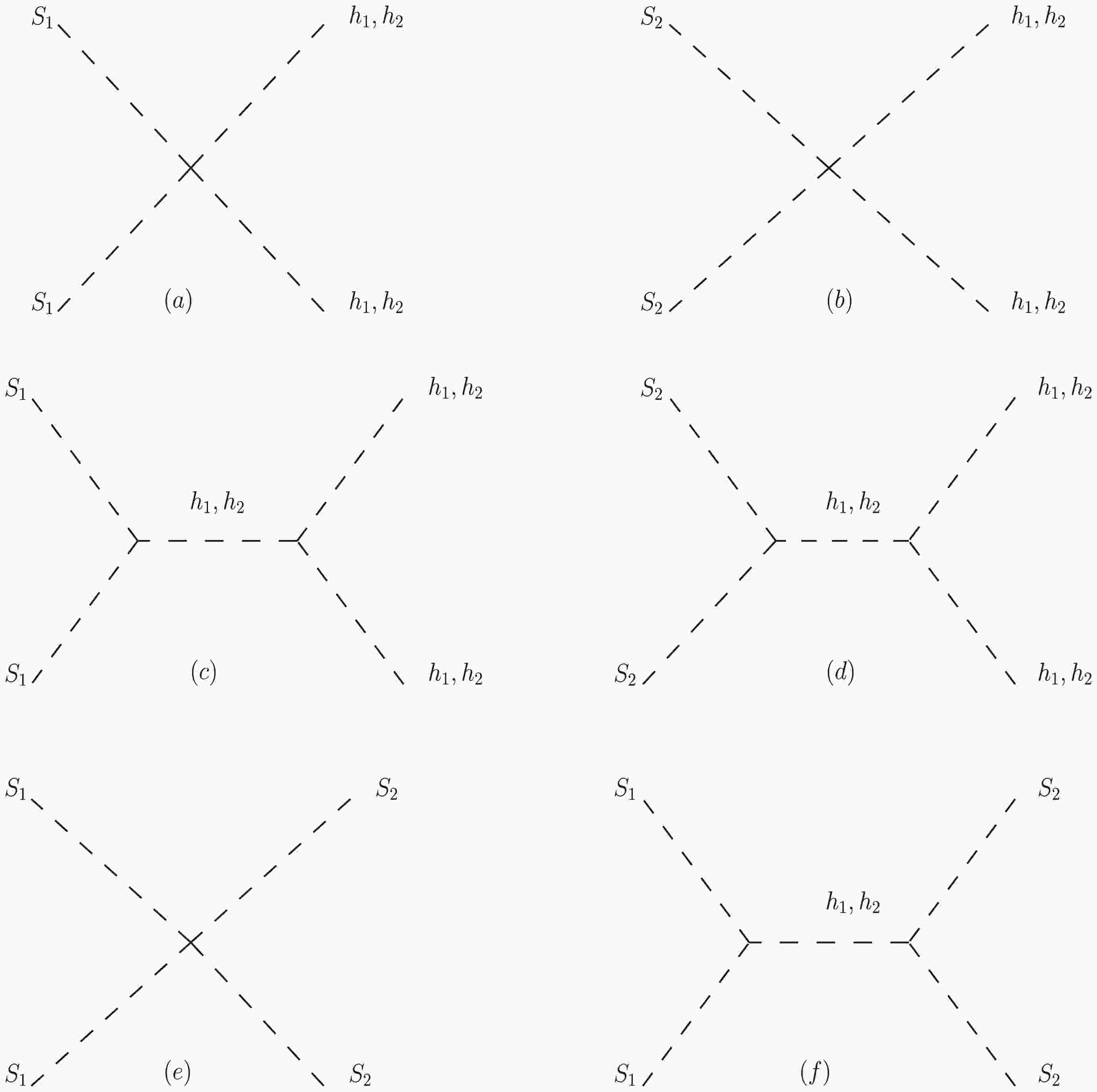
where $ n_1(n_2) $ represents the number density of $ S_1(S_2) $, $ \bar{n_1}(\bar{n_2}) $ represents the number density in thermal equilibrium, H represents the Hubble expansion rate of the Universe, X represents SM particles, and $ \langle \sigma v \rangle $ represents the thermally averaged annihilation cross section. In Fig. 1, we show the Feynman diagrams of DM annihilation processes related to new particles. Both $ S_1 $ and $ S_2 $ can be dominant in the DM relic density because of the exchange symmetry, which depends on the mass heirarchy between $ S_1 $ and $ S_2 $. The lighter one is dominant because a heavy component can annihilate into the lighter component. To calculate the DM relic density numerically, we use the micrOMGEAs 5.0.6 package [33], wherein the model is implemented through the FeynRules package [34].

Figure 1.  Feynman diagrams of DM annihilation processes related to new particles.

DM can scatter the nuclei with Higgs-mediated t-channel processes, which are constrained by the direct detection results. The effective Lagrangian related to DM-quark elastic scattering can be given by [35]

where $ {\cal{C}}_{h_1SS} $ and $ {\cal{C}}_{h_2SS} $ represent the couplings of dark matter $ S_{1,2} $ with $ h_{1,2} $ and

The expression of the cross-section for the spin-independent DM-nucleon elastic scattering can be given as [36]

where $ m_N $ represents the nucleon mass, and $ f_N $ represents the Higgs-nucleon form factor with $ f_N = 0.308(18) $ based on the phenomenological and lattice-quantum chromodynamics calculations [37]. We have two DM particles in the model, and therefore, we compare the value of $ \xi_i \sigma_{S_i N } $ against the direct detection constraints provided by the experiment results instead of the cross-section, where $ \xi_i $ represents a fraction of $ S_i $ in the total relic density defined by

where $ \Omega_{\rm DM} $ represents the observed value of the DM density and $ \Omega_i $ represents the density of $ S_i(i = 1,2) $. In our analysis, we consider the current direct detection limit set by the LZ results [38].

We estimate the parameter space in terms of the copositive criteria and DM phenomenology related to relic density and direct detection constraints. The direct detection constraint is more stringent on the low mass region, and we focus on the TeV scale DM mass in this study, where indirect detection constraints cause slight differences on the parameter space. There are eight cases related to copositive criteria based on the sign of the parameters, and each case corresponds to a viable parameter space limited by the relic density constraint and direct detection constraint. Regardless of the symmetric matrix $ {\cal{S}} $ with permutation $ \lambda_{ij} = \lambda_{ji} $, we can have different results when indices i, j, k, and l consider different permutations only for one case. Hence, discussions about the parameter space are complex for the different permutations of indices, and all possible cases should be considered to obtain the viable parameter space.

We first estimate the parameters to simplify the discussion. In this study, we select the following parameters as inputs.

$ \lambda_{33} $, $ \lambda_{34} $, and $ \lambda_{44}(\lambda_H) $ can be obtained from Eq. (8). $ \lambda_{34} $ represents the coupling of the new Higgs particles, which causes a slight difference in the DM results. Further, $ v_1 $, $ \sin\theta $, and $ m_{h_2} $ can be fixed such that $ \lambda_{33},\lambda_{34} $, and $ \lambda_{44}(\lambda_H) $ are obtained explicitly. The self-interaction couplings $ \lambda_{11} $ and $ \lambda_{22} $ slightly affect DM production, and we fix $ \lambda_{11} = \lambda_{22} = \pi $ for the sake of simplicity. Therefore, we can just consider the signs of $ \lambda_{12},\lambda_{13},\lambda_{23},\lambda_{14},\lambda_{24} $. We have an exchange symmetry of $ \lambda_{13} \leftrightarrow \lambda_{23} $, $ \lambda_{14} \leftrightarrow \lambda_{24} $, and $ S_1 \leftrightarrow S_2 $ because of the $ Z_2 \times Z_2'\times Z_2'' $ symmetry, and there is no preference for the permutations of the indexes. The five couplings can be grouped as $ \lambda_{12} $, $ (\lambda_{13},\lambda_{14}) $, and $ (\lambda_{23},\lambda_{24}) $.

The direct detection result yields the most stringent constraint on the parameter space. In Fig. 2, we obtain the viable parameter space of $ (\lambda_{13},\lambda_{14}) $ satisfying the direct detection constraint with $ m_1 = 1 $ TeV in the absence of $ S_2 $. In $ \lambda_{14} $, the coupling of SM Higgs with $ S_1 $ is limited within a narrow region under a direct detection constraint while the value of $ \lambda_{13} $ is more flexible. For a heavier $ m_1 $, a similar allowed region for $ (\lambda_{13},\lambda_{14}) $ can be obtained based on the expression of DM-nucleon elastic scattering. A negative (positive) $ \lambda_{13} $ always demands a negative (positive) $ \lambda_{14} $ for a large $ |\lambda_{13}| $, whereas the small values of $ |\lambda_{13}| $ and $ |\lambda_{14}| $ make DM production over-abundant even though the parameter space is under a direct detection constraint. Therefore, one can conclude that $ \lambda_{13} $ and $ \lambda_{14} $ consider the same signs under the direct detection constraint, which is true for $ \lambda_{23} $ and $ \lambda_{24} $ because of the exchange symmetry. Further, we are left with $ 7( = 2^3-1) $ cases to be discussed, where the cases $ \lambda_{12},\lambda_{13},\lambda_{14},\lambda_{23} $, $ \lambda_{24}\leqslant 0 $ are excluded according to the copositive criteria. Owing to the exchange symmetry, the parameter space of $ (\lambda_{13},\lambda_{14}) $ and $ (\lambda_{23},\lambda_{24}) $ can be similar, and therefore, we can consider one case to decrease the complexity and simplify the discussion. Thus, in the following discussion, we focus on the viable parameter space of $ (\lambda_{13},\lambda_{14}) $ but fix $ \lambda_{23} $ and $ \lambda_{24} $ to be constants. We discuss five cases: (1) $ \lambda_{12},\lambda_{13},\lambda_{14},\lambda_{23},\lambda_{24} \geqslant 0 $; (2) $ \lambda_{12},\lambda_{23},\lambda_{24}\geqslant 0, \lambda_{13},\lambda_{14}\leqslant 0 $; (3) $ \lambda_{12}\geqslant 0,\lambda_{13},\lambda_{14}, \lambda_{23}, \lambda_{24}\leqslant 0 $; (4) $ \lambda_{12},\lambda_{13},\lambda_{14}\leqslant 0, \lambda_{23},\lambda_{24} \geqslant 0 $; and (5) $ \lambda_{12}\leqslant 0, \lambda_{13},\lambda_{14},\lambda_{23}, \lambda_{24}\geqslant 0 $. Case (5) always satisfies the copositive criteria because $ \lambda_{11}\lambda_{22} -\lambda_{12}^2 \geqslant 0 $ always holds, and there is no difference between Cases (1) and (5) when considering the copositive criteria. Therefore, we ignore Case (5) and focus on the first four cases.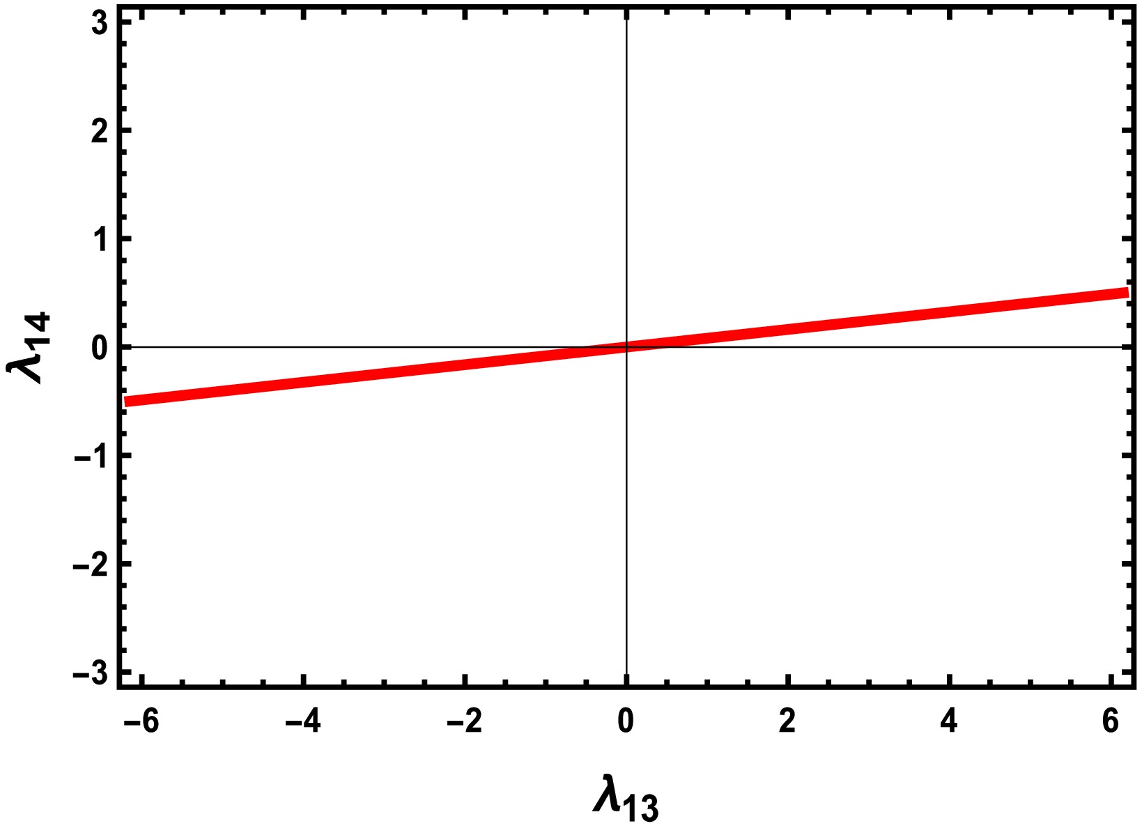

Figure 2.  (color online) Viable parameter space of $(\lambda_{13},\lambda_{14})$ under the direct detection constraint in the absence of $S_2$ with $m_1= 1$ TeV.

We discuss the four different cases with the theoretical constraints of the copositive criteria. Case (1) corresponds to Case I in Sec. III where all couplings are larger than zero. Case (2) corresponds to Case IV with $ \lambda_{13},\lambda_{14}\leqslant 0 $, and the copositive criteria demand that

Case (3) corresponds to Case VI with $ \lambda_{12},\lambda_{13},\lambda_{14}\leqslant 0 $, and the copositive criteria demand that

Case (4) belongs to Case VIII with $ \lambda_{12}\geqslant 0, \lambda_{13},\lambda_{14},\lambda_{23},\lambda_{24}\leqslant 0 $, and we can define

Therefore, the copositive criteria demands that

The copositive criteria can place stringent constraints on the parameter space to obtain a stable vacuum, and different copositive criteria are expected to contribute to different viable parameter spaces that depend on the signs of quartic couplings.

We discuss the copositive criteria, DM relic density, and direct detection constraint on the model. We consider the four different cases of the copositive criteria and focus on the viable parameter space of $ (\lambda_{13},\lambda_{14}) $. We fix $ v_1 = 2 $ TeV, $ m_{h_2} = 1.5 $ TeV, and $ \sin\theta = $ 0.01 so that we can obtain $ \lambda_{33} = 0.2812 $, $ \lambda_{34} = 0.0454 $, and $ \lambda_{44} = 0.1309 $. In addition, we set $ |\lambda_{12}| = 1 $ and $ m_2 = 3.5 $ TeV and fix $ \lambda_{23} $ and $ \lambda_{24} $ as constants. We select a small $ \sin\theta $ so that the contribution of $ S_iS_i \to h_1h_2 (i = 1,2) $ is suppressed. The expression of processes related to DM production in the limit of $ \sin\theta \to 0 $ can be found in Appendix (A4). We randomly scan the parameter space with

In our scans, we consider the model compatible with the observed DM relic density if the value, as given by micrOMEGAs, lies between 0.119 and 0.121.

In Fig. 3, we present the results of Case (1), where we set $ \lambda_{12} = 1 $ and $ \lambda_{13},\lambda_{14} \geqslant 0 $. According to Fig. 3(a), we fix $ \lambda_{23} = 3.14, \; \lambda_{24} = 0.0787 $, wheraes in Fig. 3(b), we set $ \lambda_{23} = 2.4, \; \lambda_{24} = 0.0603 $. The value of $ \lambda_{24} $ is the upper bound obtained by the DM direct detection constraint in the absence of $ S_1 $. The colored lines correspond to a viable parameter space of $ (\lambda_{13},\lambda_{14}) $, which satisfies the relic density constraint with $ m_1 = 1,2,3 $ TeV. The respective dashed lines are the upper bound of $ \lambda_{14} $ arising from the direct detection constraint. The region of the colored lines below the representative dashed lines correspond to the parameter space satisfying both the relic density and direct detection constraint. The direct detection result puts the most stringent constraint on the parameter space. $ \lambda_{13} $ is related to processes involving $ h_2 $, while $ \lambda_{14} $ is related to processes involving SM Higgs ($ h_1 $). According to Fig. 3, when $ \lambda_{13} $ is small, the value of $ \lambda_{14} $ is approximately equal to a constant larger than 0.1 under the relic density constraint, which means the processes related to $ h_1 $ are dominant over DM production while the processes related to $ h_2 $ are less efficient. With an increase in $ \lambda_{13} $, $ \lambda_{14} $ decrease sharply as long as $ \lambda_{13} $ is approximately equal to 1, where processes related to $ h_2 $ are so efficient that $ \lambda_{13} $ is constrained strictly and $ \lambda_{14} $ has a lower bound. Direct detection constraint excludes the region that $ \lambda_{13} $ is considerably smaller than 1, which indicates that $ h_2 $ plays an important role in determining DM production within the viable parameter space. For the heavier $ m_1 $ with $ m_1 = 2 $ and 3 TeV, the upper bound of $ \lambda_{13} $ is larger to obtain the correct relic density as the lower bound of $ \lambda_{14} $ is larger. However, in the case of $ m_1 = 1 $ TeV smaller than $ m_{h_2} $, the process of $ S_1S_1 \to h_2 h_2 $ is highly suppressed, and $ \lambda_{13} $ should be considerably larger to meet the relic density constraint. The lower bound of $ \lambda_{14} $ is larger according to Fig. 3(a). In Fig. 3(b) with $ \lambda_{23} = 2.4,\lambda_{24} = 0.0603 $, we obtain a similar conclusion, wherein the viable value of $ \lambda_{13} $ is at the$ {\cal{O}}(1) $ level. However, the lower bound of $ \lambda_{14} $ is considerably larger because the density of $ S_2 $ is larger in this case, and we require a stronger interaction related to $ S_1 $ to obtain the correct relic density.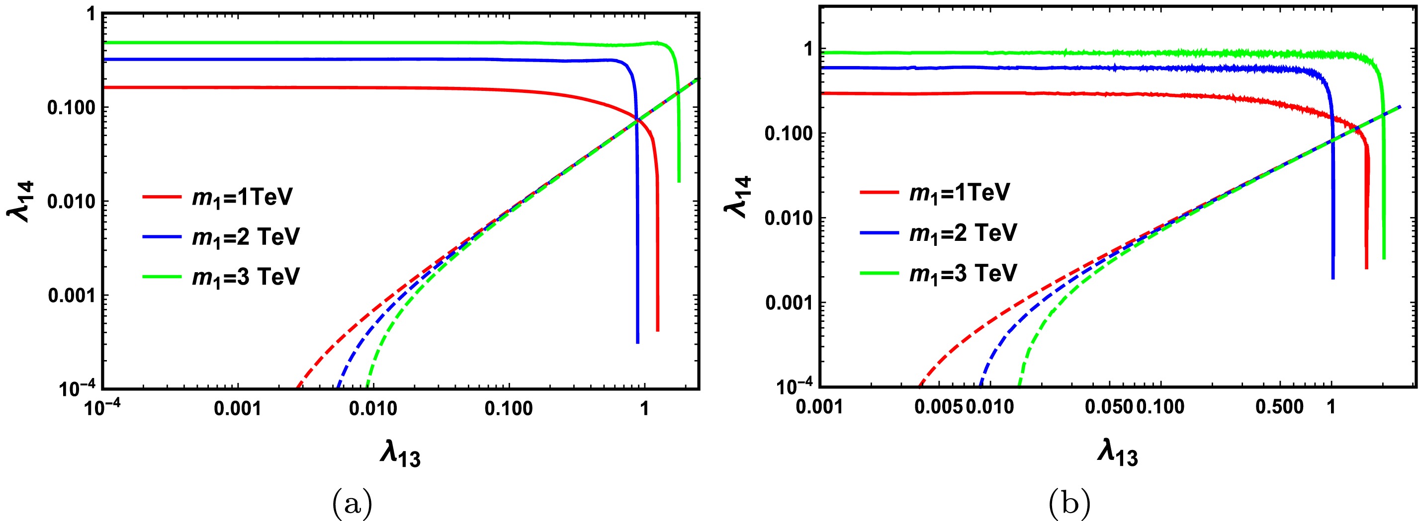

Figure 3.  (color online) Results of Case (1) with $\lambda_{12}=1,\lambda_{13},\lambda_{14} \geqslant 0$, where we fix (a) $\lambda_{23}=3.14,\lambda_{24}=0.0787$ and (b) $\lambda_{23}=2.4,\lambda_{24}=0.0603$. The colored lines correspond to the viable parameter space of $(\lambda_{13},\lambda_{14})$ satisfying the relic density constraint with $m_1=1,2,3$ TeV, and the respective dashed lines are the upper bound of $\lambda_{14}$ arising from the direct detection constraint.

We present the results of Case (2) in Fig. 4 with $ \lambda_{12} = 1, \lambda_{13},\lambda_{14} \leqslant 0 $, where we fix (a) $ \lambda_{23} = 3.14,\lambda_{24} = 0.0787 $ and (b) $ \lambda_{23} = 2.4,\lambda_{24} = 0.0603 $. The colored lines correspond to the viable parameter space of $ (|\lambda_{13}|, \, |\lambda_{14}|) $ satisfying a relic density constraint with $ m_1 = 1,2,3 $ TeV, and the respective dashed lines represent the upper bound of $ |\lambda_{14}| $ arising from direct detection constraint. The blue-shadowed region corresponds to the parameter space satisfying the copositive criteria. The cross-section of $ S_iS_i \to h_i h_i(i = 1,2) $ is determined by the Higgs-mediated processes, and therefore, the quartic term $ |S_i|^2|h_i|^2 $ and t-channel processes exchange by DM, where the sign of the couplings $ \lambda_{13} $ and $ \lambda_{14} $ can create differences in the interference terms of these diagrams. Thus, the viable parameter space is different. According to Fig. 4(a), the smaller $ |\lambda_{13}| $ is excluded for DM density being over-abundant because of the interference effect. Similarly, the viable $ |\lambda_{13}| $ value is constrained within a narrow region while the $ |\lambda_{14} $ value is more flexible; however, it sharply decreases with an increase in $ |\lambda_{13}| $ by the direct detection constraint as the results of Case (1), where $ h_2 $ plays a dominant role in determining DM production. For a larger $ m_1 $, the upper bound of $ |\lambda_{13}| $ is considerably smaller to obtain the correct relic density compared to that of the results of Case (1) in Fig. 3(a) because of the interference effect. In addition, the copositive criteria in Case (2) can constrain the parameter space strictly and for $ m_1 = 1 $ TeV. The allowed $ (|\lambda_{13}|,|\lambda_{14}|) $ is almost excluded as shown in Fig. 4(a). For Fig. 4(b) with $ \lambda_{23} = 2.4, \lambda_{24} = 0.0603 $, the copositive criteria naturally exclude a small $ |\lambda_{13}| $ from the point of the theoretical constraint in the case of $ m_1 = 3 $ TeV. Further, for $ m_1 = 1 $ TeV, the allowed parameter space of $ (|\lambda_{13}|,|\lambda_{14}|) $ are completely excluded by the copositive criteria.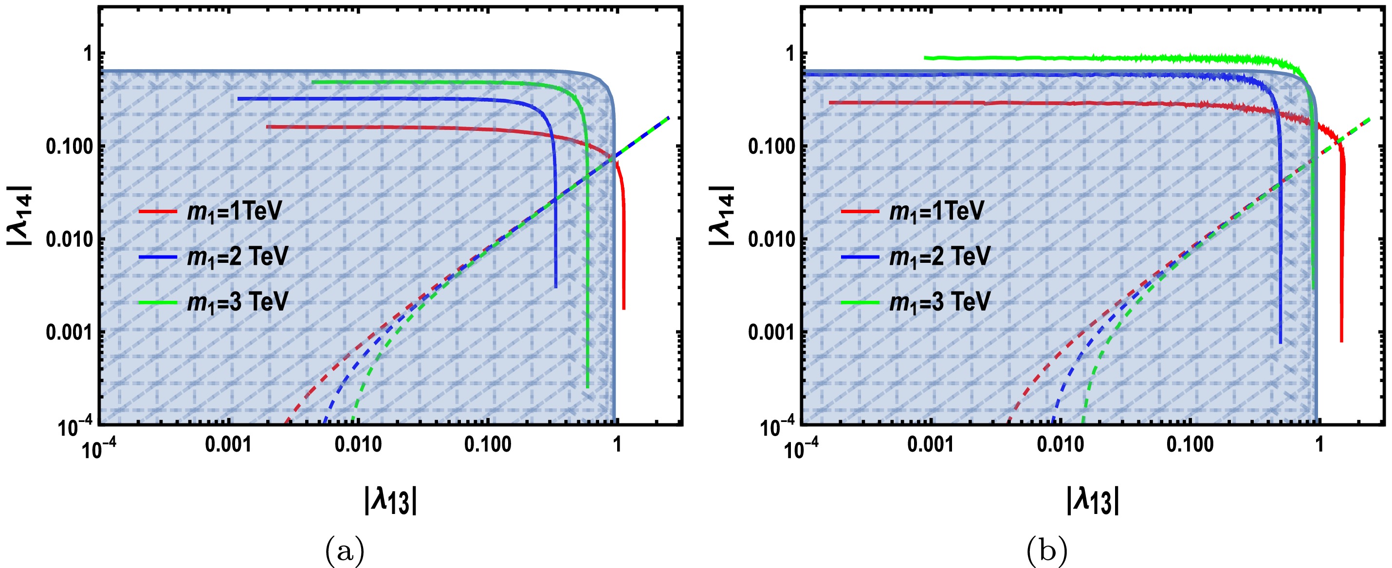

Figure 4.  (color online) Results of Case (2) with $\lambda_{12}=1,\lambda_{13},\lambda_{14} \leqslant 0$, where we fix (a) $\lambda_{23}=3.14,\lambda_{24}=0.0787$ and (b) $\lambda_{23}=2.4, $$ \lambda_{24}=0.0603$. The blue-shadowed region corresponds to the parameter space satisfying the copositive criteria of Case (2). The colored lines correspond to the viable parameter space of $(|\lambda_{13}|,|\lambda_{14}|)$ satisfying the relic density constraint with $m_1=1,2,3$ TeV, and the respective dashed lines are the upper bound of $|\lambda_{14}|$ arising from the direct detection constraint.

In Figs. 5(a) and (b), we present the results of Case (3) with $ \lambda_{12} = -1,\lambda_{13},\lambda_{14} \leqslant 0 $, where we fix $ \lambda_{23} = 3.14, \lambda_{24} = 0.0787 $ in (a) and $ \lambda_{23} = 2.4,\lambda_{24} = 0.0603 $ in (b). The difference between Cases (3) and (2) is $ \lambda_{12} $, set to a negative value, and the combined contribution of the Higgs-mediated processes and quartic term $ S_1^2S_2^2 $ will determine the cross-section of $ S_1S_1 \to S_2S_2 $. The sign of $ \lambda_{12} $ affects the interference terms; however, such interactions between $ S_1 $ and S₂ just adjust the relative relic density of $ S_1 $ and $ S_2 $, which makes a slight difference in the viable parameter space of $ \lambda_{13} $ and $ \lambda_{14} $. Therefore, we obtain similar results for Case (2) as we can see in Figs. 5(a) and (b).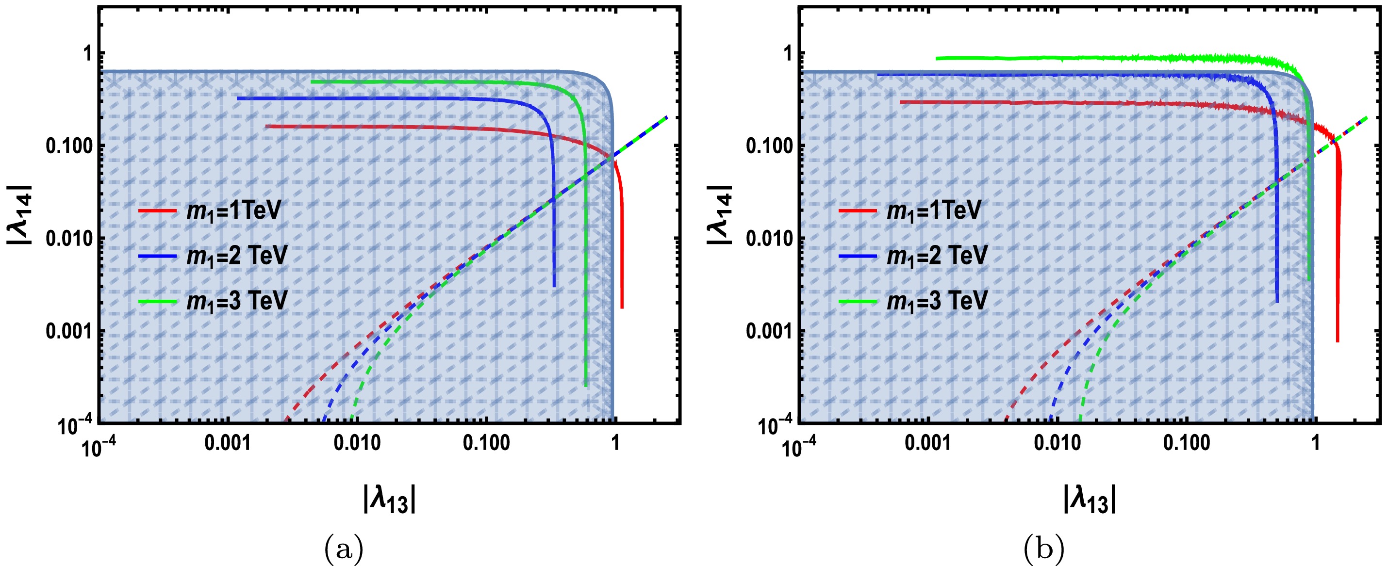

Figure 5.  (color online) Results of Case (3) with $\lambda_{12}=-1,\lambda_{13},\lambda_{14} \leqslant 0$, where we fix (a) $\lambda_{23}=3.14,\lambda_{24}=0.0787$ and (b) $\lambda_{23}=2.4, $$ \lambda_{24}=0.0603$. The blue-shadowed region corresponds to the parameter space satisfying the copositive criteria of Case (3). The colored lines correspond to the viable parameter space of $(|\lambda_{13}|,|\lambda_{14}|)$ satisfying the relic density constraint with $m_1=1,2,3$ TeV, and the respective dashed lines represent the upper bound of $|\lambda_{14}|$ arising from the direct detection constraint.

We present the results of Case (4) in Fig. 6 with $ \lambda_{12} = 1, \lambda_{13}, \; \lambda_{14} , \; \lambda_{23}, \; \lambda_{24} \leqslant 0 $ The value of $ \lambda_{23} $ and $ \lambda_{24} $ are also constrained according to the copositive criteria of Case (8). Within the selected parameter space, one can obtain $ |\lambda_{23}|\leqslant 0.94 $ and $ |\lambda_{24}|\leqslant 0.64 $ with Eq. (21). In Fig. 6(a), we fix $ \lambda_{23} = -0.9 $ and $ \lambda_{24} = -0.023 $, and the allowed values of $ |\lambda_{13}| $ and $ |\lambda_{14}| $ are completely excluded by the direct detection constraint and copositive criteria within the selected parameter space in the case of $ m_1 = 1 $ TeV. For $ m_1 = 3 $ TeV, the allowed value of $ |\lambda_{14}| $ is more flexible because of the interference effect. We set $ \lambda_{23} = -0.75 $ and $ \lambda_{24} = -0.194 $ in Fig. 6(b), where the copositive criteria exclude the parameter space of $ (|\lambda_{13}|,|\lambda_{14}|) $ in the case of not only $ m_1 = 1 $ TeV but also $ m_1 = 3 $ TeV regardless of the direct detection constraint.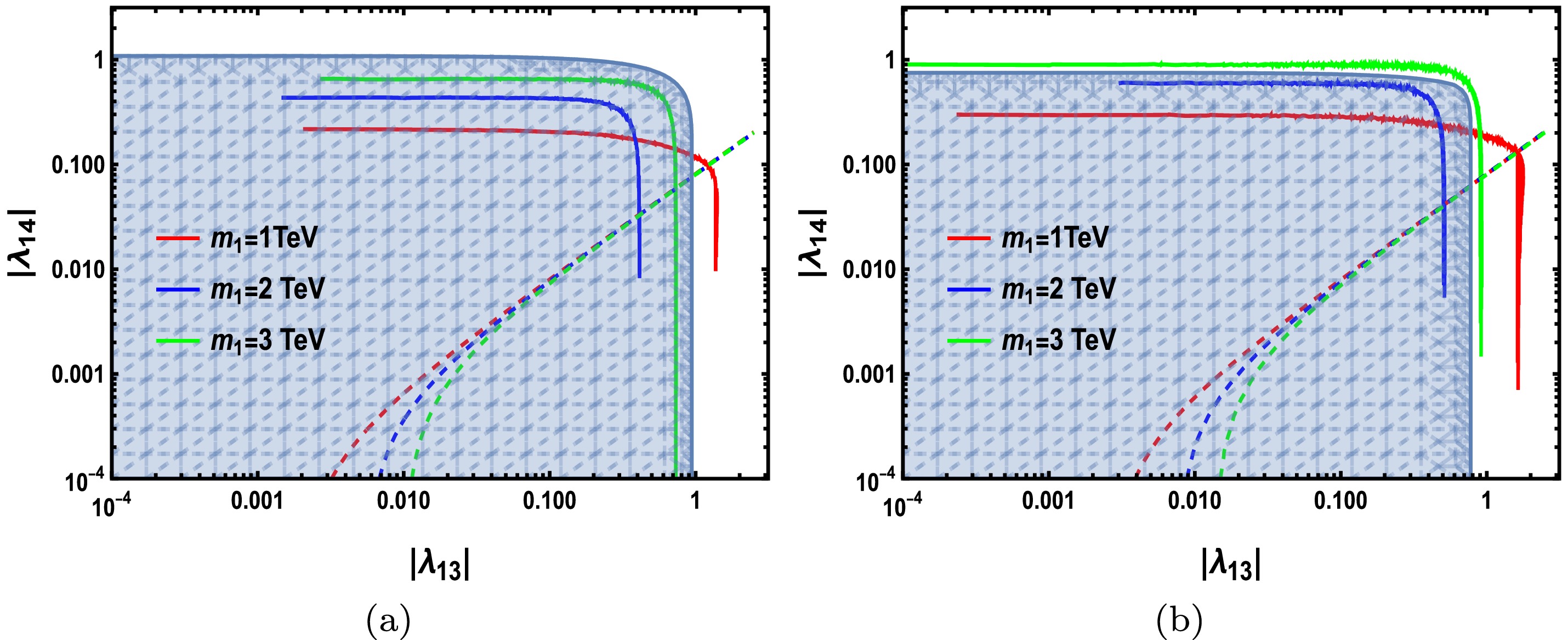

Figure 6.  (color online) Results of Case (4) with $\lambda_{12}=1,\lambda_{13},\lambda_{14},\lambda_{23},\lambda_{24}\leqslant 0$, where we fix (a) $\lambda_{23}=-0.9,\lambda_{24}=-0.023$ and (b) $\lambda_{23}=-0.75, $$ \lambda_{24}=-0.194$. The blue-shadowed region corresponds to the parameter space satisfying the copositive criteria of Case (3). The colored lines correspond to the viable parameter space of $(|\lambda_{13}|,|\lambda_{14}|)$ satisfying the relic density constraint with $m_1=1,2,3$ TeV, and the respective dashed lines represent the upper bound of $|\lambda_{14}|$ arising from the direct detection constraint.

According to Figs. 3 to 6, we show the effect of the copositive criteria on the parameter space. Different choices of the signs of couplings can contribute to different copositive conditions, which can induce different viable parameter spaces caused by the interference effect. Further, we consider four different cases and randomly scan the selected parameter space under DM relic density and direct detection constraints. Direct detection constraint places the most stringent limit on the parameter space, requiring the new Higgs $ h_2 $ to play a dominant role in determining DM relic density. The copositive criteria can also constrain the allowed parameters space such that the case of $ m_1 = 1 $ TeV is excluded for different copositive conditions when some of the couplings are negative. When we consider $ \lambda_{12} = 1,\lambda_{13},\lambda_{14} \leqslant 0, \lambda_{23} = -0.75 $ , and $ \lambda_{24} = -0.194 $, the copositive criteria are more stringent on the viable parameters, and the parameter space of $ m_1 = 3 $ TeV is completely excluded regardless of the direct detection constraint. The high values of the couplings $ \sim 1 $ can indicate a low energy validity for the model with two stable scalars, which is expected to set limitations for the model at high energies. In the appendix, we perform a random scan and present viable parameter spaces with four different cases satisfying the copositive criteria, relic density, and direct detection constraint. According to the results, the allowed values for the couplings can be obtained at the $ {\cal{O}}(0.1) $ level, which are appropriate with a high scale validity of the model.

WIMPs as DM face serious challenges in that no signals have been found in direct detection experiments so far, and therefore, one solution to such a problem is the multi-component DM model, which includes two or more DM species. The multi-component DM model is constrained by theoretical and experiment constraints. For the extended scalar DM models, vacuum stability requires the scalar potential to be bounded from below, which can place stringent constraints on the parameter space. Further, the copositive criteria enable deriving the necessary and sufficient analysis conditions for vacuum stability of the couplings. Different copositivity criteria can contribute to different viable parameter spaces depending on the choice of the signs of the couplings.

We considered a two-component scalar DM model in this study. The $ 4\times 4 $ matrix of the quadratic couplings must satisfy the copositivity criteria to obtain stable vacuum. Provided the direct detection results place stringent constraints on the parameter space, the discussion on the related parameters can indeed be simplified greatly, and we focus on four different cases related to copositive criteria based on the signs of quadratic couplings in the model. The signs of these parameters will not only demand different copositivity criteria but also affect the results of the cross-section of the $ 2 \to 2 $ processes and induce a different viable parameter space caused by the interference effect. We randomly scanned the selected parameter space with DM relic density and direct detection constraints. For the four different cases, the allowed values of $ (|\lambda_{13}|,|\lambda_{14}|) $ are different; however, they demand the new Higgs $ h_2 $ to play a dominant role in determining the DM relic density within the viable parameter space. Further, we perform a random scan in the appendix under DM relic density and direct detection constraints; a few points "survive" when copositive criteria are considered. For different criteria, the allowed values for the couplings are different according to the results. Thus, the copositive criteria can place stringent constraints on the parameter space as long as some quartic coupling is negative.

The different choices of the signs of couplings can contribute to different parameter spaces with the copositive criteria. The model in this study is simple, but the discussion about the copositive criteria is complex because of the different permutations of the indices. For a more complex model, the copositivity enables us to find the necessary and sufficient analysis conditions to ensure vacuum stability so that the parameter space can be theoretically estimated.

To ensure the perturbative model, the contribution from loop correction must be smaller than the tree level values, and such constraints can be ensured with

Unitarity conditions arise from the tree-level scalar-scalar scattering matrix, which is dominated by the quartic contact interaction. The s-wave scattering amplitudes should lie under the perturbative unitarity limit, given the requirement that the eigenvalues of the S-matrix $ {\cal{M}} $ must be less than the unitarity bound given by $ |\mathrm{Re}{\cal{M}}| < \dfrac{1}{2} $.

In this section, we present the renormalization group equations of the model with SARAH [39] at a one-loop level. The beta functions of the quartic couplings are given by

where $ y_t $ represents the Top Yukawa coupling, and $ g_1 $ and $ g_2 $ represent the gauge couplings of $ U(1) $ and $ S U(2) $.

We consider the cross section of $ S_iS_i \to h_ih_i $ and $ S_iS_i \to h_1h_2 $ $ (i = 1,2) $ in this section. We calculate the cross section using Calchep [40]. The expressions in the limit of $ \sin\theta\to 0 $ are given as

According to the expressions of the cross-section, in the limit of $ \sin\theta \to 0 $, the signs of $ \lambda_{13} $, $ \lambda_{23} $, $ \lambda_{14} $, and $ \lambda_{24} $ can lead to differences in the terms, including the odd orders of these couplings that contribute to the cross-section of $ S_iS_i \to h_ih_i (i = 1,2) $. For non-zero $ \sin\theta $, the signs of $ \lambda_{13} $, $ \lambda_{23} $, $ \lambda_{14} $, and $ \lambda_{24} $ can lead to differences in the cross section because of the combined contributions of these couplings such as $ \lambda_{13}\lambda_{24} $.

In this section, we perfrom a random scan on the selected parameter space with

We fix $ \sin\theta = 0.01, m_{h_2} = 1.5 $ TeV, and $ v_1 = 2 $ TeV for simplicity. We consider the copositive criteria, DM relic density, and direct detection constraint on the model for the four different cases. The results are presented in Figs. A1 to A4.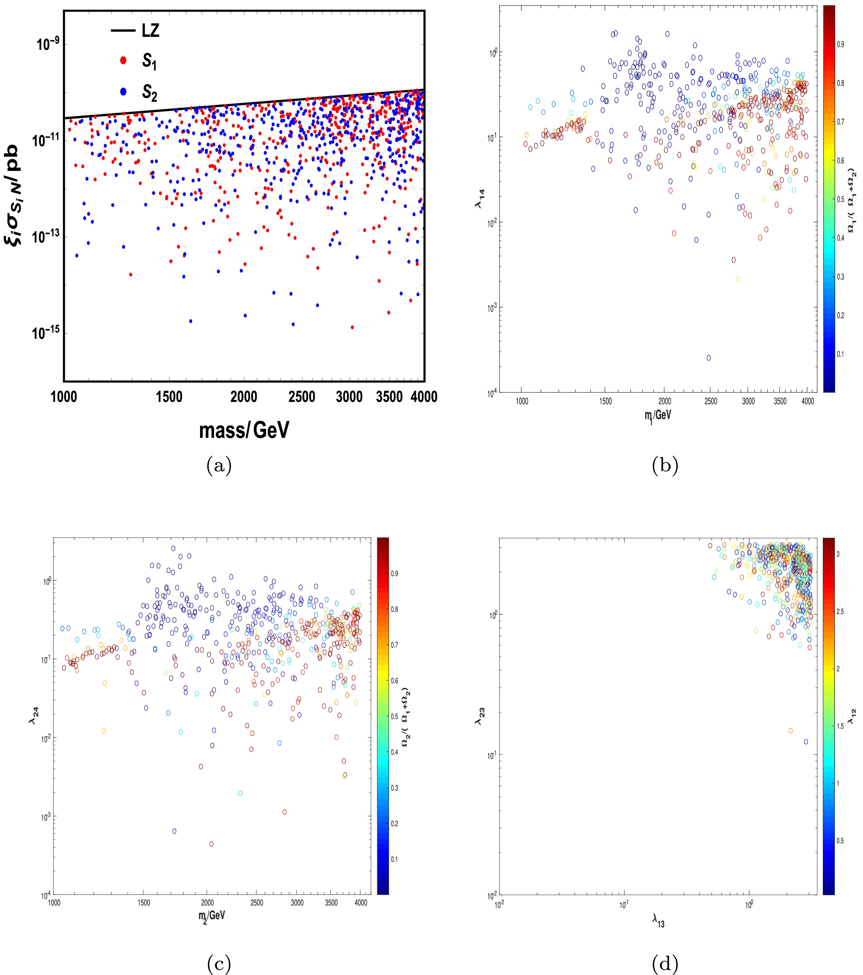

Figure A1.  (color online) Results of the viable parameter space satisfying the relic density and direct detection constraint for Case (1). (a) Allowed values for DM mass $S_1$(red points) and $S_2$ (blue points); the black line represents the upper bound according to the latest LZ results. (b) Viable parameter space for $m_1-\lambda_{14}$, where bubbles with different colors correspond to the fraction of $S_1$ defined by $\Omega_1/(\Omega_1+\Omega_2)$. (c) Viable parameter space for $m_2-\lambda_{24}$, where bubbles with different colors correspond to the fraction of $S_2$ defined by $\Omega_2/(\Omega_1+\Omega_2)$. (d) Allowed values for $\lambda_{13}-\lambda_{23}$, where bubbles with different colors represent the viable values for $\lambda_{12}$.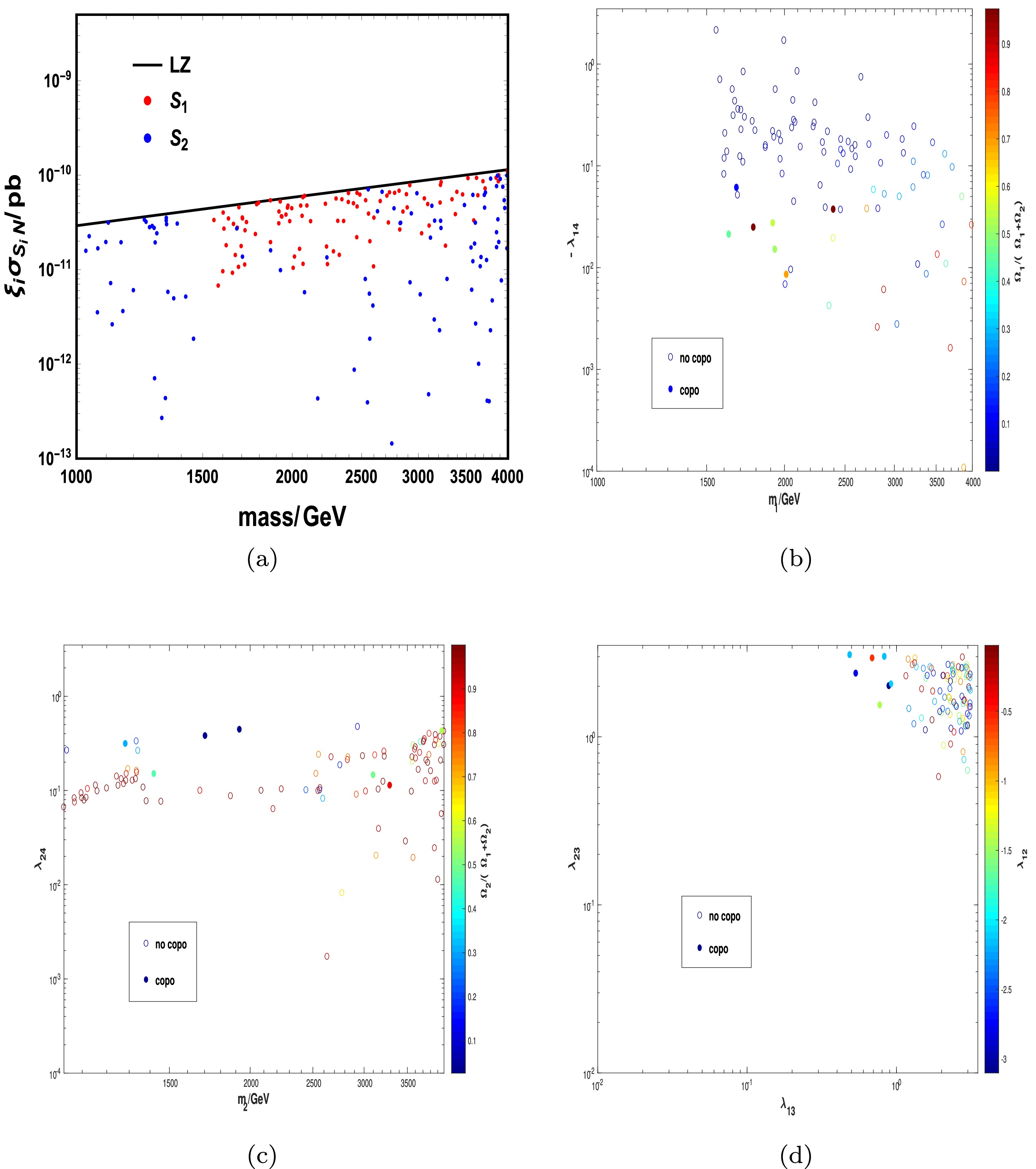

Figure A2.  (color online) Results of viable parameter space satisfying the relic density and direct detection constraint for Case (2). In (b), (c), and (d), the colored points satisfy the copositive criteria, whereas the colored bubbles do not; they are labeled as "copo" and "no copo," respectively.

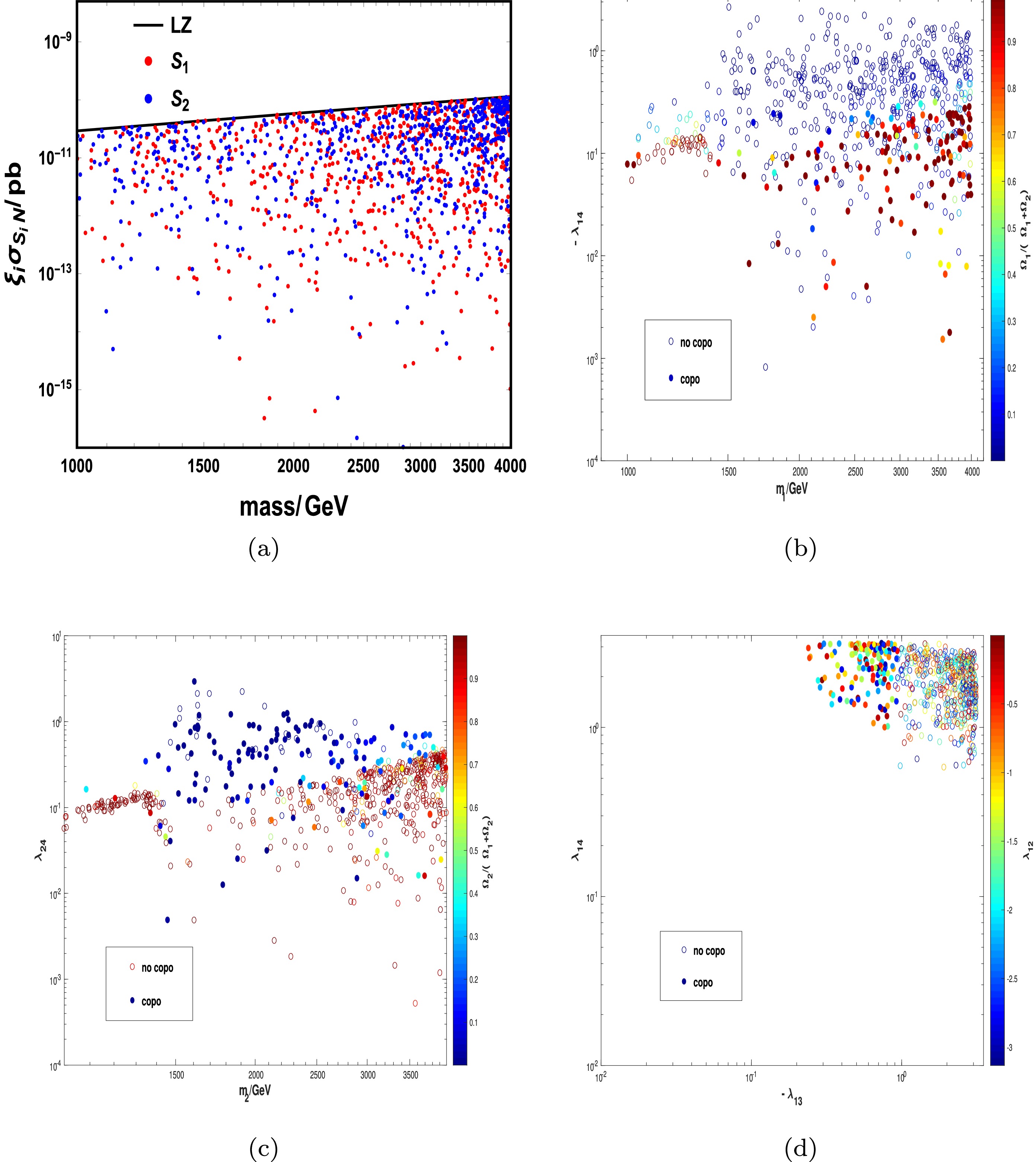
Figure A3.  (color online) Results of viable parameter space satisfying the relic density and direct detection constraint for Case (3). In (b), (c), and (d), the colored points satisfy the copositive criteria, whereas the colored bubbles do not; they are labeled as "copo" and "no copo," respectively.

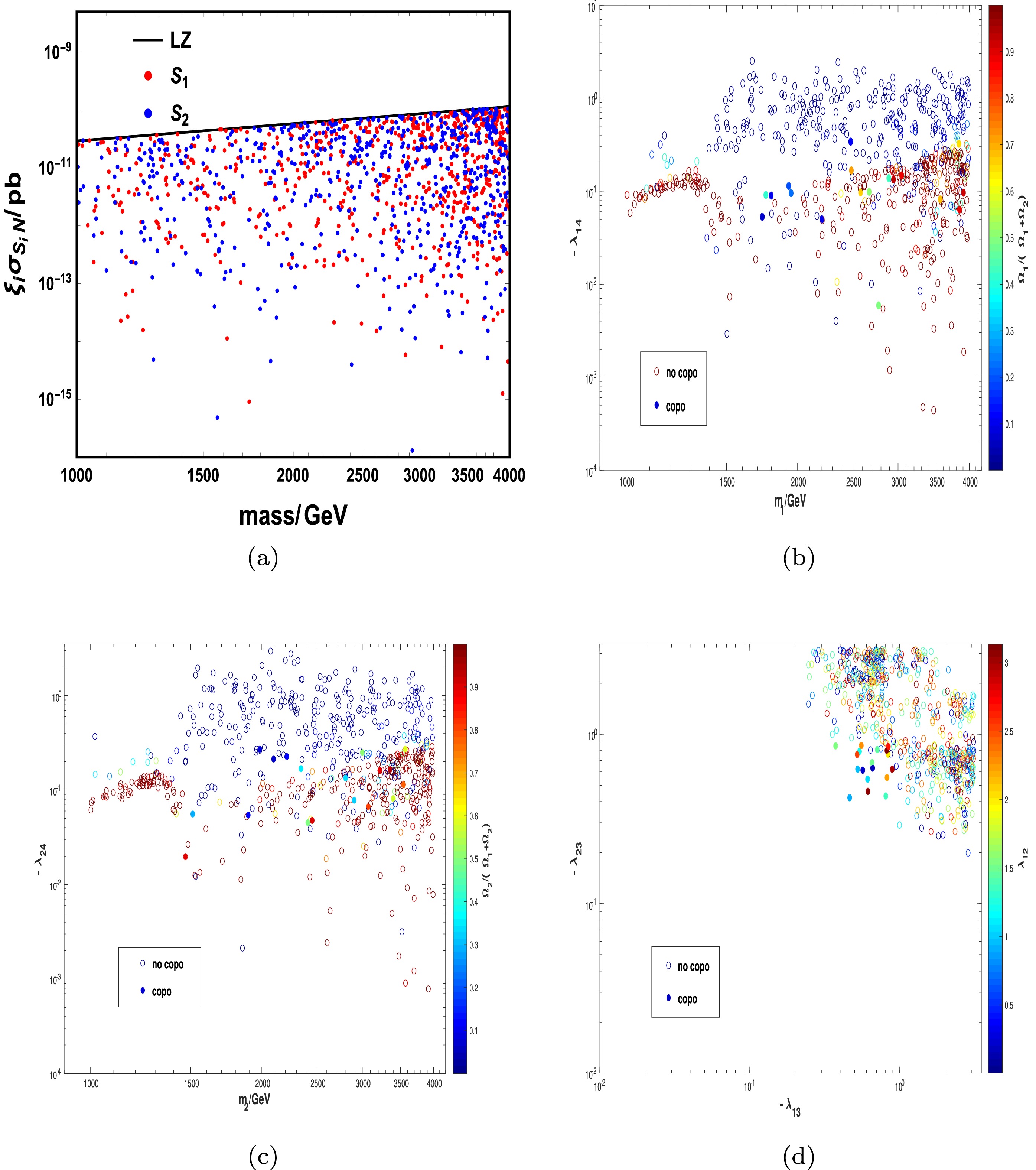
Figure A4.  (color online) Results of the viable parameter space satisfying the relic density and direct detection constraint for Case (4). In (b), (c), and (d), the colored points satisfy the copositive criteria, whereas the colored bubbles do not. They are labeled as "copo" and "no copo," respectively.

For Case (1), the copositive criteria result in a slight difference in the parameter space, and the viable parameter space satisfies the relic density and direct detection constraint as indicated in Fig. A1. Both $ m_1 $ and $ m_2 $ can have values in the range of [1 TeV, 4 TeV], as shown inFig. A1(a). According to (b) and (c), a larger $ \lambda_{14} $ ($ \lambda_{24} $) can contribute to a stronger interaction rate such that the fraction of $ S_1 $ ($ S_2 $) is smaller. The direct detection constraint limits $ \lambda_{14} $ and $ \lambda_{24} $ to be small, and large $ \lambda_{13} $ and $ \lambda_{23} $ are therefore required under the relic density constraint. Fig. A1(d) shows that most of the points lie in the upper right region for $ (\lambda_{13},\lambda_{23}) $. In addition, $ \lambda_{12} $ is related to the conversion processes between $ S_1 $ and $ S_2 $, which is less constrained.

For Cases (2), (3), and (4), we consider the copositive criteria on the parameter space. The viable parameter space satisfying the relic density and direct detection constraint is shown in Figs. A2, A3, and A4, where the colored points satisfy the copositive criteria, whereas the colored bubbles do not. They are labeled as "copo" and "no copo," respectively. We obtain a similar conclusion for Case (1); however, when considering the copositive criteria, the parameter space is more constrained, and only a few points "survive" according to Figs. A2 to A4. In addition, for the different copositive criteria, the allowed parameter spaces are different.