Fermion masses and mixing in SO(10) GUT with a universal two-zero texture

The flavor puzzle is a long-standing unresolved problem in particle physics. We are still unclear on the reason for the large difference between lepton and quark mixings or whether the many independent mixing parameters could be correlated through an underlying mechanism beyond the Standard Model (SM).

The texture-zero approach [1−3], which was first proposed to calculate the Cabibbo angle and reduce free parameters in the quark sector, provides an efficient approach to address the flavor puzzle. This approach assumes that some entries of the quark Yukawa matrices (or equivalently, mass matrices) vanish, and the approach connects quark masses with the CKM mixing parameters. Thus, the number of free parameters for quark flavors is efficiently reduced. A competitive pattern is the so-called four texture zeros [4−6], in which both up- and down-type quark Yukawa matrices are Hermitian and their (1,1) and (1,3) entries are zeros:

for $ f = u,d $, where the $ (3,1) $ entry is also zero owing to the assumption of Hermitian Yukawa matrices. This is a natural extension of the original Fritzsch texture, which includes a third zero in the (2,2) entry [7−9]. This texture features analytical simplicity [10, 11] and can be employed for solving the strong CP problem [12]; see Ref. [13].

Texture zeros have been applied to the lepton sector by first assuming the light neutrino mass matrix taking the form of Eq. (1) expressed in the charged lepton flavor basis [14−16]. A universal two-zero texture (UTZT) in the lepton sector, i.e., both $ M_l $ and $ M_\nu $ have two zero entries in the same position, was proposed in [17]. The lepton flavor model with the UTZT in the seesaw framework was constructed in [18] within the context of Abelian discrete symmetries [19].

Both four texture zeros in the quark sector and the UTZT in the lepton sector have fit the relevant flavor data accurately so far. Motivated by their phenomenological successes, we propose unified two-zero textures in both the quark and lepton sectors, representing completely universal two-zero textures for all fermion mass matrices. Specifically, the subscript f in Eq. (1) will span for all quarks and leptons. To achieve this, we propose to work within the GUT framework. The grand unified version of the UTZT has another advantage. It helps to reduce the large dimensionality of the parameter space in the flavor space. We assume the gauge symmetry to be $ S O(10) $ [20] and exploit one of its key features: all quarks and leptons including the right-handed neutrino are assigned in the same sixteen-dimensional chiral representation. As a consequence, strong corrections of masses and mixing of all quarks and leptons are predicted [21, 22]; see Refs. [23−26] , which consider recent precision data.

The proposed model is constructed in $ S O(10) \times Z_6 $ with the Pati-Salam symmetry [27] as an intermediate symmetry after GUT breaking and before its breaking to the SM gauge symmetry. The texture zeros are realized in $ Z_6 $ symmetry following the method developed in [18]. Abelian discrete symmetries have been applied for realizing flavor texture zeros in GUT models [28−31].

The rest of this paper is organized as follows. In Sec. II, we construct the UTZT in $ S O(10) $ GUTs with a $ Z_6 $ flavor symmetry. In Sec. III, we discuss the analytical properties of the UTZT in GUTs and report on the numerical analysis of fermion masses and mixing. In Sec. IV, we explore the parameter space of intermediate scales allowed by gauge unification and proton decay constraints under a certain breaking chain from $ S O(10) $ to SM, where different copies of Higgs fields introduced along with $ Z_6 $ are considered. We conclude the paper with Sec. V.

We construct the UTZT for fermion masses with the gauge and flavor symmetries assumed to be $ S O(10) $ and $ Z_6 $, respectively. We focus on the breaking chain,

where symbols above and below each arrow refer to the energy scale of the corresponding symmetry breaking and the Higgs multiplet responsible for the breaking, respectively, and $ Z_2^{\rm{C}} $ is the parity symmetry between left particles and right charge-conjugate particles. All particle arrangements in $ S O(10) \times Z_6 $ and the corresponding roles are listed in Table 1. In addition, a CP symmetry, which will be spontaneously broken later, is introduced above the GUT scale. Next, we first review some general features of fermion masses in $ S O(10) $ and then discuss the construction of the UTZT by imposing a $ Z_6 $ flavor symmetry.

	Particles in $S O(10)$	Charges in $Z_6$	Roles in the theory
Fermions	$({\bf{16}}_F^1, {\bf{16}}_F^2, {\bf{16}}_F^3)$	$\{ 0,2,1 \}$	Contains SM fermions & RH neutrinos
Higgses	$({\bf{10}}_H^1, {\bf{10}}_H^2, {\bf{10}}_H^3)$	$\{ 4,3,2 \}$	Generates fermion masses
	$({\bf{120}}_H^1, {\bf{120}}_H^2, {\bf{120}}_H^3)$	$\{ 4,3,2 \}$	Generates fermion masses
	$(\overline{\bf{126}}_H^1, \overline{\bf{126}}_H^2, \overline{\bf{126}}_H^3)$	$\{ 4,3,2 \}$	Generates fermion masses & triggers LR symmetry breaking
	${\bf{54}}_H$	0	Triggers GUT symmetry breaking
	${\bf{45}}_H$	0	Triggers PS symmetry breaking

Table 1.  Particle content in $S O(10) \times Z_6$.

In $ S O(10) $ GUTs, all fermions, including quarks and leptons as well as right-handed neutrinos, are introduced to explain light neutrino masses and unified in a single matter field multiplet $ {\bf{16}} $ of $ S O(10) $. The matter field multiplet follows the representation product decomposition $ {\bf{16}} \times {\bf{16}} = {\bf{10}}_{\rm{S}} + \overline{\bf{126}}_{\rm{S}} + {\bf{120}}_{\rm{A}} $, where subscripts S and A correspond to symmetric and anti-symmetric combinations. To generate $ S O(10) $-invariant Yukawa interaction, three Higgs multiplets are included, $ {\bf{10}}_H $, $ \overline{\bf{126}}_H $, and $ {\bf{120}}_H $. In general, Yukawa couplings to generate fermion masses can be arranged as

where $ \alpha,\beta = 1,2,3 $ denote three copies of flavors. In general, A, B, and C are $ 3 \times 3 $ coupling matrices, with A and B being symmetric and C being antisymmetric. The CP symmetry requires them to be real, as explained below; otherwise, they are complex. Here, we do not consider copies of the Higgs in the flavor space; these are specified in the next subsection. We work within the non-SUSY framework. The complex conjugates of $ {\bf{10}}_H $ and $ {\bf{120}}_H $ transform as $ {\bf{10}} $- and $ {\bf{120}} $-plets of $ S O(10) $. In the case that both $ {\bf{10}}_H $ and $ {\bf{120}}_H $ are real, Eq. (3) provides the most general Yukawa couplings in $ S O(10) $. If $ {\bf{10}}_H $ and $ {\bf{120}}_H $ are complex, there might be additional couplings

appearing in the Lagrangian. In this case, we forbid them by imposing an additional Peccei-Quinn (PQ) $ U(1) $ symmetry [32], as described in [33−35]. In each case, Eq. (3) (following the proof in Appendix A) leads to Dirac Yukawa coupling matrices taking the following structure [21, 22, 36, 37]:

where H and F are symmetric matrices, whereas G is an antisymmetric matrix. H, F, and G are identical to $ A^* $, $ B^* $, and $ C^* $, respectively, up to the overall coefficients, if both $ {\bf{10}}_H $ and $ {\bf{120}}_H $ are real. These Yukawa coupling matrices are expressed in the left-right convention given that we are working within the non-supersymmetric GUT framework. Dirac masses for quarks and leptons are obtained after Higgses gain VEVs. The light neutrino mass matrix $ M_\nu $ is obtained from the Type-(I+II) seesaw mechanism,

where $ m_L $ and $ m_R $ are free and small mass parameters induced by Higgs VEVs. Here, we have parameterized the RH neutrino mass matrix as

It is convenient to express Yukawa coupling terms in the Pati-Salam notation. In $ S U(4)_c \times S U(2)_L \times S U(2)_R \subset S O(10) $, the $ {\bf{16}}_F $ fermion multiplet of $ S O(10) $ is decomposed into two multiplets of the Pati-Salam gauge symmetry. These multiplets are denoted as $ \psi_L $ and $ \psi_R^{\rm{C}} $, respectively, and

where $ {\rm{C}} $ in the superscript of a fermion represents charge conjugation. All Higgs multiplets are decomposed into bi-doublets of $ S U(2)_L\times S U(2)_R $. More explicitly,

In Eqs. (8) and (9), a and b denote entries of the $ S U(4)_c $ fundamental representation, and i and j denote entries of $ S U(2)_L $ and $ S U(2)_R $ fundamental representations, respectively. In the Pati-Salam symmetry, the Yukawa coupling terms, e.g., $ (A)_{\alpha\beta} \; {\bf{16}}^\alpha_F {\bf{16}}^\beta_F {\bf{10}}_H + {\rm i}\, (C)_{\alpha\beta} \; {\bf{16}}^\alpha_F {\bf{16}}^\beta_F {\bf{120}}_H + {\rm{h.c.}} $, are reduced to

where $ \epsilon = {\rm i}\,\sigma_2 $ has been used for singlet contraction from two doublets of $ S U(2) $. The $ S O(10) $ gauge symmetry includes an internal matter parity symmetry $ Z_2^{\rm{C}} $. This parity is also called D parity in the reference. Explicit rules of the parity transformation in SO(10) and Pati-Salam group theories are reported in [38] and not repeated here. Generally, this parity in $ S U(2)_L \times S U(2)_R $ appears to be the following transformation:

We impose a CP symmetry above the GUT scale. Coupling matrices A, B, and C are forced to be real in this symmetry [39]. The CP transformation in $ S U(2)_L \times S U(2)_R $ appears as

in the Pati-Salam convention, where transformation of spatial coordinates is dismissed. The CP symmetry is spontaneously broken by the VEV of $ {\bf{120}} $ [39], i.e., VEVs of $ \eta_{ij} $ and $ \tilde{\eta}^a_b{}_{ij} $. The CP symmetry combined with $ Z_2^{\rm{C}} $ forms a Klein symmetry. The latter includes an additional parity transformation:

This parity enables the permutation of left- and right-handed fermions and keeps the Yukawa couplings as Hermitian [12].

We introduce a $ Z_6 $ discrete symmetry in the flavor sector and aim to obtain the UTZT for all Yukawa matrices. In general, texture zeros can be realized in Abelian discrete flavor symmetries [19]. We follow the charge alignments given in [18] by assuming a $ Z_6 $ flavor symmetry. In a straightforward extension, we extend each Higgs multiplet into three copies, e.g., $ {\bf{10}}^k_H $ for $ k = 1,2,3 $, etc. The renormalizable Yukawa couplings in Eq. (3) are then extended into

for $ k = 1,2,3 $, where $ A_k $, $ B_k $ , and $ C_k $ are all $ 3 \times 3 $ coupling matrices with $ A_k $ and $ B_k $ being symmetric and $ C_k $ being antisymmetric. We consider to arrange $ Z_6 $ charges for both matter and Higgs fields as

for $ \alpha,k = 1,2,3 $, respectively. To be invariant under $ Z_6 $, all non-vanishing couplings in these terms should take zero charge (mod 6). We checked each term in Eq. (14) to determine whether such a condition is satisfied. We conclude that coupling matrices take the following textures:

Here, a cross represents a non-vanishing entry in the matrix, referring to a zero $ Z_6 $ charge in the relevant Yukawa coupling.

We checked whether the UTZT is satisfied in all fermion Yukawa/mass matrices. All Dirac Yukawa coupling matrices $ Y_f $ (for $ f = u,d,e,\nu $) are linear combinations of the matrices in Eq. (16). Thus, they take forms of two-zero flavor textures, as in Eq. (1). Note that these matrices are Hermitian as the CP symmetry is imposed. In the neutrino sector, the Majorana mass matrix for the RH neutrino $ M_R $ is a linear combination of $ B_1 $, $ B_2 $, and $ B_3 $. It is a real and symmetric matrix with two-zero texture, as in Eq. (17). All Yukawa matrices can be explicitly expressed as

where $ f = u,d,\nu,e $, the entries $ A_f $ and $ \tilde{B}_f $ are real, and $ B_f $ and $ C_f $ are complex. We keep $ A_f >0 $ by extracting a sign parameter $ \zeta_f = \pm 1 $ out.

For the light neutrino mass matrix $ M_\nu $, one can demonstrate using the Type-(I+II) seesaw formula in Eq. (6) that the light neutrino mass matrix inherits the textures in Eq. (17) through the Type-(I+II) seesaw mechanism [40, 41]. However, $ M_\nu $ is not Hermitian but complex and symmetric.

Before ending this section, we discuss other possibilities to realize the UTZT through discrete symmetries. We first prove that, given the PQ $ U(1) $ symmetry, three copies of Higgs constitute the minimal requirement. Indeed, given any $ Z_n $ symmetry with fermion $ {\bf{16}}_F^\alpha $ and Higgs $ \{{\bf{10}}, \overline{\bf{126}}, {\bf{120}} \}^k_H $ charges arranged with $ q^F_\alpha $ and $ q^H_k $ (both $ q^F_\alpha $ and $ q^H_k $ are integers less than n), the two-zero textures can be achieved by applying the algebras described next. For any Higgs, their charges $ q^H_k $ must satisfy

and there must be some Higgses with charges $ q^H_{k_1} $, $ q^H_{k_2} $,..., satisfying

To distinguish flavors, $ q^F_1 \neq q^F_2 \neq q^F_3 \neq q^F_1 $ (mod n) and $ n \geqslant 3 $. Taking this property into the above equation, we obtain

This means that $ q^H_{k_1} $, $ q^H_{k_2} $, and $ q^H_{k_3} $ as well as $ q^H_{k_2} $, $ q^H_{k_3} $, and $ q^H_{k_4} $ should be distinguishable charges. In the minimal case, $ q^H_{k_1} = q^H_{k_4} $, and as a consequence, we are left with three copies of Higgses. Although three copies are the minimal requirement for the UTZT, there are plenty of choices for $ Z_n $ and charged assignments to satisfy the algebras described by Eqs. (18) and (19). In particular, $ Z_6 $ is not unique in achieving the texture alignment. For example, $ Z_5 $ can realize the UTZT with matter and Higgs fields arranged as

In the case without PQ symmetry, the number of Higgs copies can be reduced to two. This is because $ {\bf{10}}^*_H $ and $ {\bf{120}}^*_H $ join in the Yukawa couplings, as in Eq. (4). The three different charges, $ q^H_{k_1} $, $ q^H_{k_2} $ , and $ q^H_{k_3} $, can be arranged as follows: two of them are charges of two distinguishable Higgses, and the third charge refers to the charge conjugation of one of these Higgses. Applying this argument to our $ Z_6 $ model in Eq. (15), the third copy of Higgses is not necessary because it can be replaced by the charged conjugation of the first copy. Regarding the $ Z_5 $model in Eq. (21), the third copy is not necessary either because it can be replaced by the charge conjugation of the second copy. Reducing the copy of Higgses results in additional restriction on the Yukawa correlation between quarks and leptons, which is worth studying in the future.

In this section, we discuss correlations between masses and mixing of quarks and leptons both analytically and numerically. The heavy neutrino masses required to generate light neutrino data via the seesaw mechanism are also predicted.

A remarkable advantage of the two-zero texture is its analytical calculability, which enables us to diagonalize the Yukawa matrices analytically in terms of the eigenvalues and largest entry of the Yukawa matrix [11]. Given that all fermions are embedded in the same $ S O(10) $ multiplet, all fermion masses are correlated. It is a non-trivial task to match fermion masses and mixing with their experimental data. We present Eq. (5) again in the following form:

where $ r_1\, {\rm{Im}} Y_u = r_3\, {\rm{Im}} Y_d $ is satisfied. Restricted by the $ Z_6 $ symmetry, all Dirac Yukawa coupling matrices$ Y_f $ are Hermitian with two texture zeros, i.e.,

where $ f = u,d,\nu,e $; $ A_f $ and $ \tilde{B}_f $ are real; $ B_f $ and $ C_f $ are complex; $ A_f>0 $; and $ \zeta_f = \pm1 $. The light neutrino mass matrix $ M_\nu $ and heavy neutrino mass matrix $ M_R $ are given in Eqs. (6) and (7), with

The resulting $ M_\nu $ is a complex symmetric $ 3\times 3 $ matrix with two-zero textures, and $ M_R $ is real.

We parameterize the quark sector as follows. In the Yukawa matrix $ Y_u $, which is in general complex, a minus sign of $ B_u $ or $ C_u $ can be rotated away by performing phase rotation with a phase π. This transformation does not change the real property of F, H, and G. With a phase rotation $ P_u = {\rm{diag}} \{ 1, {\rm e}^{{\rm i} \phi_u}, {\rm e}^{{\rm i} \phi_u^\prime} \} $, the Hermitian Yukawa matrix $ Y_u $ can be transformed into a real and symmetric matrix:

Without loss of generality, we can set $ \zeta_u = +1 $, and $ \tilde{B}_u $ could be either positive or negative. They are correlated with up-type quark Yukawa couplings as follows [10, 13]:

where $ \eta_u = \pm 1 $ is an undetermined sign. The real orthogonal matrix, which is used in the diagonalization

with $ \hat{Y}_u = {\rm{diag}}\{ -\eta_u y_u, \eta_u y_c, y_t\} $, can be explicitly expressed in terms of $ A_u $, $ y_u $, $ y_c $, and $ y_t $ as [10, 13]

The down-type quark Yukawa matrix $ Y_d $ is in general complex. With a phase rotation $ P_d = {\rm{diag}}\{ 1, {\rm e}^{{\rm i} \phi_d}, {\rm e}^{{\rm i} \phi_d^\prime} \} $, it can be transformed into a real and symmetric matrix:

On the right-hand side, one can perform a transformation similar to that for $ Y_u $ with the orthogonal matrix $ O_d $ given by

Specifically,

where $ \hat{Y}_d = {\rm{diag}}\{ -\eta_d y_d, \eta_d y_s, y_b\} $. The CKM mixing matrix is given by

It is useful to parameterize $ A_u $ and $ A_d $ again in the form $ A_u = y_t (r + \epsilon) $ and $ A_d = y_b (r - \epsilon) $. From numerical analysis, we found that, to satisfy experimental data, the restriction $ |\epsilon| < 0.03 $ must be satisfied. From experimental quark data, the following hierarchical relations exist among mixing parameters:

where $ \theta_C $ is the Cabibbo angle. Using these relations, we approximately derive the three mixing angles as

where $ \phi_1 = \phi_u-\phi_d,\, \phi_2 = \phi_u^\prime-\phi_d^\prime $. According to Eq. (22), $ Y_e $ can be expressed in terms of $ Y_u $ and $ Y_d $ with coefficients $ r_1 $, $ r_2 $ , and $ c_e $. The entries of $ Y_e $ satisfy correlations similar to those in Eq. (26),

where $ A_e $ is the absolute value of the $ (3,3) $ entry of $ Y_e $. This parameterization simplifies the numerical analysis presented in the next subsection.

In the neutrino sector, however, $ M_\nu $ is a complex and symmetric matrix, and the phase rotation cannot transform $ M_\nu $ into a real matrix. The unitary matrix to diagonalize $ M_\nu $ has to be obtained numerically. For RH neutrinos, the Majorana mass matrix $ M_R $, which is proportional to F as a linear combination of $ {\rm{Re}}\, Y_u $ and $ {\rm{Re}}\, Y_d $, is a real matrix with two texture zeros. It can be analytically diagonalized by a real orthogonal matrix $ O_R $, which takes a form similar to that of $ O_{u,d,e} $ but replacing the Yukawa couplings by relevant RH neutrino masses $ M_{N_1} $, $ M_{N_2} $, and $ M_{N_3} $; it is not repeated here.

We describe our numerical analysis in this subsection. To simplify the analysis, we fix the numerical best-fit (bf) values of the charged fermion Yukawa couplings,

We do not consider the errors for these values, which means that the pulls for all charged fermion Yukawa couplings are explicitly fixed at zero. Best-fit and $ 1\sigma $ values of three mixing angles and one CP-violating phase in the CKM mixing matrix are assumed to be

These values were calculated at the GUT scale ($ 2\times 10^{16} $ GeV) from a non-SUSY scenario, as reported in [42].

In the quark sector, because the condition $ r_1\, {\rm{Im}} Y_u = r_3\, {\rm{Im}} Y_d $ is always satisfied, which means that $ \dfrac{ {\rm{Im}} ({\rm{Y}}_{\rm{u}})_{12}}{ {\rm{Im}} ({\rm{Y}}_{\rm{d}})_{12}} = \dfrac{ {\rm{Im}} ({\rm{Y}}_{\rm{u}})_{23}}{ {\rm{Im}} ({\rm{Y}}_{\rm{d}})_{23}} =\dfrac{r_3}{r_1} $, the value of $ \phi_d^\prime $ is fully determined by $ \{\phi_u, \phi_u^\prime, \phi_d\} $. Once Yukawa couplings $ y_f $ for $ f = u,c,t,d,s,b $ are fixed at their best-fit values, $ Y_u $ and $ Y_d $ are fully determined by the free parameters $ \{A_u, A_d, \phi_1, \phi_2 \} $ up to the sign parameters $ \{\eta_u, \eta_d, \zeta_u, \zeta_d\} $, where $ \zeta_u = 1 $ is fixed without loss of generality; $ \zeta_d $ does not influence masses and mixing in the quark sector but contributes to the lepton sector via Eq. (22). We explore the following intervals:

After $ Y_u $ and $ Y_d $ are determined by the above fitting procedure in the quark sector, all non-vanishing entries of $ Y_e $, i.e., $ A_e $, $ B_e $, $ \tilde{B}_e $ and $ C_e $, become functions of $ r_1 $, $ r_2 $, and $ c_e $. We fix $ y_e $, $ y_\mu $, and $ y_\tau $ at their best-fit values, and $ r_1 $, $ r_2 $, and $ c_e $ are determined with the help of Eq. (35) up to a sign difference $ \eta_e $. Then, $ Y_e $ is fixed, and we can determine the unitary matrix $ U_e $ in the diagonalization $ U_e^\dagger Y_e U_e = \text{diag}\{y_e,y_\mu,y_\tau\} $.

In the neutrino sector, according to Eq. (22), the only undetermined parameter in $ Y_\nu $ is $ c_\nu $. In Eq. (6), the light neutrino mass matrix, $ M_\nu $, is determined by two additional parameters, $ m_L $ and $ m_R $. We explore these parameters in the following regions:

using the logarithmic scale to obtain $ M_\nu $. Then, the diagonalization $ V_\nu^\dagger M_\nu V_\nu^* = \text{diag}\{m_1,m_2,m_3\} $ provides the neutrino mass eigenvalues and unitary matrix $ V_\nu $. Finally, the PMNS matrix is given by $ U_{\rm{PMNS}} = V_e^\dagger V_\nu $, and the three lepton mixing angles are expressed as

On the experimental side, we used their global bf values (excluding SK atmospheric data) from NuFIT 5.3 [43, 44] ¹ and averaged the positive and negative $ 1\sigma $ errors. We also considered two mass-squared differences, $ \Delta m^2_{21} = m_2^2-m_1^2 $ and $ \Delta m^2_{31} = m_3^2-m_1^2 $

for the normal mass ordering (NO, i.e., $ m_1 < m_2 < m_3 $). The up-to-date experimental constraint on the Dirac CP-violating phase $ \delta^l $, $ \delta^l = 197^\circ \pm 41^\circ $, which is still weak, was not included in the fit. Instead, we treated $ \delta^l $ as a model prediction. We do not discuss inverted ordering (i.e., $ m_3 < m_1 < m_2 $) in this paper because a preliminary analysis suggested that our model does not favor this configuration. Furthermore, we do not consider the small flavor-dependent RG running effect owing to the suppression of the charged lepton Yukawa coupling.

We count the number of free parameters introduced in the model and the independent observables used to fit the data. Once the charged fermion masses are fixed, we are left with four free parameters $ \{A_u,\, A_d,\, \phi_1,\, \phi_2\} $ to explore and two signs $ \{\eta_u,\eta_d\} $ in the quark sector, with four observables $ \{\theta_{12}^q,\theta_{13}^q,\theta_{23}^q,\delta^q\} $ to fit. In the neutrino sector, we analyzed three free parameters $ \{c_\nu, m_L, m_R\} $ and two signs $ \{\eta_e,\zeta_d\} $, with five observables $ \{\theta_{12}^l,\theta_{13}^l,\theta_{23}^l, \Delta m^2_{21},\Delta m^2_{31}\} $ to fit.

In summary, there are seven free parameters:

These parameters were used to fit nine independent observables:

Other observables were treated as model predictions.

We conducted a simple $ \chi^2 $ analysis with the $ \chi^2 $ function defined as

where $ {\rm{obs}}_n $ denotes the nine independent observables in Eq. (43), and $ {\rm{para}}_m $ accounts for the eight free parameters in Eq. (42) with the exploration intervals defined in Eqs. (38) and (39). We determined the regions to fit the experimental data by setting an upper bound to the $ \chi^2 $ value. Our analytical procedure was divided into two steps. First, we explored the quark sector by setting $ \chi_q^2<10 $. Then, we used the quark data for further exploration aiming at finding points with $ \chi_l^2<10 $ in the charged lepton and neutrino sector. We further established that $ \chi^2 = \chi^2_q + \chi^2_l \leq 10 $ and excluded points at which $ \chi^2 > 10 $. The results are shown in Figs. 1 and 2.

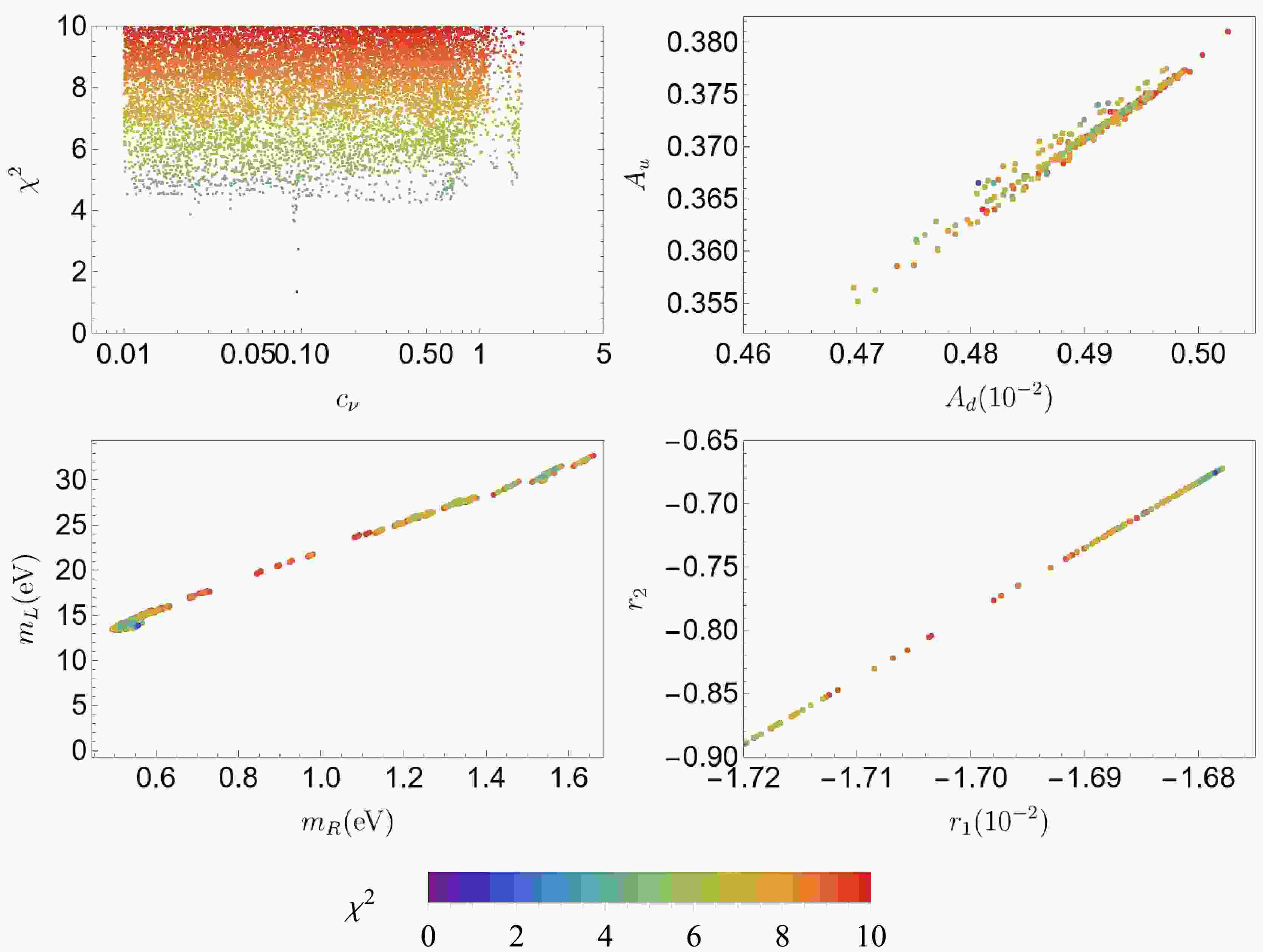
Figure 1.  (color online) Parameters for the model with $\chi^2 \leq 10$.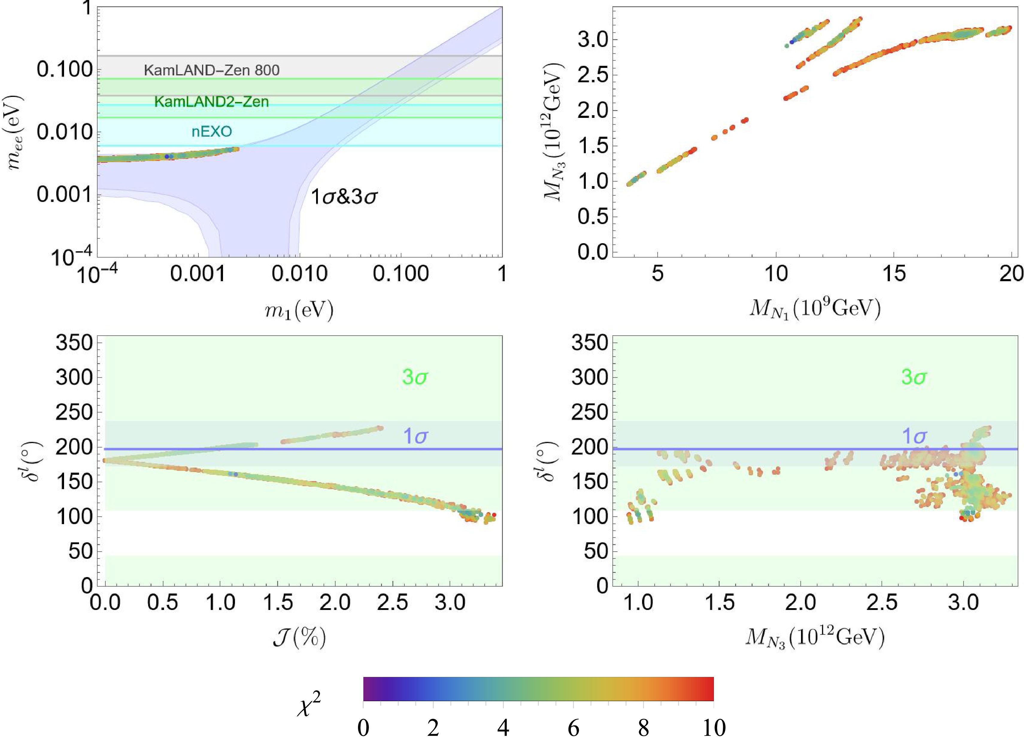

Figure 2.  (color online) Effective neutrino mass prediction (top left panel) and two-dimensional correlations between predicted observables for $\chi^2 \leq 10$.

Figure 1 shows the dependence of the $ \chi^2 $ value on the model parameters as well as correlations among these parameters. Note that $ c_\nu $ varies in the range (0,1.7) and $ \chi^2 $ reaches a minimum of 1.6 when the value of $ c_\nu $ is approximately 0.1 ². The benchmark point at the minimum of $ \chi^2 $ is listed in Appendix B.

Note also the linear correlation between $ r_1 $ and $ r_2 $. This relationship can be analytically derived with the help of Eqs. (22) and (35),

where $ X = \zeta_e[-A_e+y_\tau+\eta_e(y_\mu-y_e)]+\zeta_d[A_d-y_b+ \eta_d(y_d-y_s)],$ $Y = A_u-y_t+\eta_u(y_u-y_c), $ $ Z = \zeta_e[-A_e+y_\tau+\eta_e(y_\mu- y_e)]+3\zeta_d [-A_d+ y_b+\eta_d(y_s-y_d)] $. According to the rest of the panels in Fig. 1, the theory inputs hold the following hierarchical relation:

Figure 2 shows correlations between predicted observables. In the top left panel of Fig. 2, predictions for the effective mass $ m_{ee} $ of the neutrinoless double beta decay are represented as a function of the lightest neutrino $ m_1 $ for NO. The effective mass $ m_{ee} $ is defined as

The predicted values of $ m_{ee} $ are mostly distributed between 3.45 and 5.2 meV, and the values of $ m_1 $ are smaller than 2.33 meV. Furthermore, we calculated the CP-violating phase $ \delta_l $ and Jarlskog invariant $ \mathcal{J} $, which measures the strength of CP violation in neutrino oscillations [46, 47]. As shown in Fig. 2, the CP-violating $ \delta^l $ varies in the interval $ (90^\circ,230^\circ) $. $ \mathcal{J} $ ranges from $ 0 $% to $ 3.5 $% and clearly increases as the Dirac CP-violating phase $ \delta^l $ deviates from $ 180^\circ $. At the benchmark point, $ \delta^l $ is predicted to be $ 160^\circ $ and $ \mathcal{J} $ is equal to $ 1.14 $%. The upcoming long-base neutrino experiments DUNE [48] and Hyper-Kamiokande [49] are expected to achieve a resolution of $ \delta_l $ at the level of $ 10^\circ $. Thus, they are expected to exclude a large parameter space of this model.

Once all free parameters are determined, we can obtain the RH neutrino mass matrix through Eqs. (7) and (24), whose eigenvalues are three RH neutrinos masses, $ M_{N_1} $, $ M_{N_2} $, and $ M_{N_3} $. As shown in Fig. 2, the heaviest RH neutrino mass is predicted to be approximately $ (1\sim 3.3) \times 10^{12} $ GeV. In Section IV, we check whether this is consistent with gauge unification and proton decay constraints.

$ S O(10) $GUTs have many breaking chains. In the context of a specific breaking chain, the solutions to the RGEs and the requirement of gauge unification impose restrictions on the GUT scale and establish a correlation with the intermediate scales. Given that the proton decay rate depends on the GUT scale, we can exploit the limits on this observable to constrain the GUT scale as well as intermediate scales. Recall that our breaking chain is $ S O(10) \to G_{422}^{\rm{C}} \to G_{3221} \to G_{\rm{SM}} $, as introduced in Sec. II. In this analysis, we go beyond the hypothesis of minimal particle content and consider the influence of additional Higgses on gauge unification. The scale of the lowest intermediate symmetry breaking, denoted as $ M_1 $ in Eq. (2), refers to the $ B-L $ breaking scale. Majorana masses for right-handed neutrinos are generated after the $ B-L $ spontaneous breaking at $ M_1 $. By keeping the Yukawa couplings in the perturbative region, all right-handed neutrinos, including the heaviest one, should not have masses greater than $ M_1 $. Next, we check whether gauge unification in this model satisfies the experimental constraint from proton decay and examine whether there is any tension between the lowest intermediate scale and the predicted right-handed neutrino mass.

Any intermediate symmetry between $ S O(10) $ and SM can be expressed as a product of Lie groups $ H_1\times\dots\times H_n $; the two-loop renormalization group running equation for group $ H_i $ is given by

where $ t = \log(\mu/\mu_0) $, $ \alpha_i = g_i^2/4\pi $. The β function depends on the field contents of the theory:

Here, $ b_i $ and $ b_{ij} $ are coefficients and can be expressed as

where the ψ and ϕ indices sum over the fermions and complex scalar multiplets, respectively, and $ \psi_i $ and $ \phi_i $ are their representations in the group $ H_i $, respectively. $ C_2(R_i) $ (for $ R_i = \psi_i, \varphi_i $) represents the quadratic Casimir of the representation $ R_i $ in group $ H_i $, and $ C_2(H_i) $ is the quadratic Casimir of the adjoint presentation of the group $ H_i $. If the condition $ \dfrac{b_j}{2\pi}\alpha_j(t_0)(t-t_0)<1 $ is satisfied, these equations can be analytically solved:

The one-loop matching condition for group $ H_{i+1} $ broken into a subgroup $ H_i $ at scale $ M_I $ is given by [50] $ \alpha_{H_{i+1}}^{-1}(M_I)-\dfrac{1}{12\pi}C_2(H_{i+1}) = \alpha_{H_i}^{-1}(M_I)-\dfrac{1}{12\pi}C_2(H_i) $. When $ S U(2)_R\times U(1)_X\longrightarrow U(1)_Y $, we have the matching condition [51] $ \dfrac{3}{5}\Big(\alpha_{2R}^{-1}(M_I)-\dfrac{1}{6\pi}\Big)+\dfrac{2}{5}\alpha_{1X}^{-1}(M_I) = \alpha_{1Y}^{-1}(M_1) $. In this breaking pattern, $ {\bf{54}}_H,{\bf{45}}_H,{\bf{10}}_H,\overline{\bf{126}}_H,{\bf{120}}_H $ are needed to trigger symmetry breaking and generate fermion masses. In the following, $ n_H $ is used to represent the repetition number of the Higgs field $ {\bf{10}}_H,{ \overline{{\bf{126}}}}_H,{\bf{120}}_H $, and the copy of $ {\bf{54}}_H,{\bf{45}}_H $ is always set to one. For $ M_2\to M_{\rm{GUT}} $, we assume that only $ ({ {\bf{15}},{\bf{1}},{\bf{1}}})\subset {\bf{45}}_H $ contributes to RG running, given that it is responsible for the symmetry breaking from $ S U(4)_c \times S U(2)_L \times S U(2)_R \times Z_2^{\rm{C}} $ to $ S U(3)_c \times S U(2)_L \times S U(2)_R \times U(1)_X $, and other components of $ {\bf{45}}_H $ are assumed to be around the GUT scale. Therefore, when $ n_H = 0 $, we have the following β-coefficients:

The final β-coefficients can be obtained from $ b_i = b_i^0+ n_H\delta b_i,b_{ij} = b_{ij}^0+n_H\delta b_{ij} $. Next, we analyze three scenarios where unification constraints are notably different.

$ {\rm{S1}}) $ We assume that the components of the Higgs multiplets that are unnecessary for symmetry breaking at lower scales are heavy and decouple at higher scales. Minimal Higgs content for each intermediate symmetry breaking is considered. Specifically, Higgs contents include $({{\bf{1}},{\bf{2}},{\bf{2}}})\subset {\bf{10}}_H $, $ ({{\bf{15}},{\bf{2}},{\bf{2}}})+({ \overline{{\bf{10}}},{\bf{3}},{\bf{1}}})+({{\bf{10}},{\bf{1}},{\bf{3}}})\subset { \overline{{\bf{126}}}}_H $, $ ({{\bf{1}},{\bf{2}},{\bf{2}}}) + ({{\bf{15}},{\bf{2}},{\bf{2}}}) \subset {\bf{120}}_H $ in $ G_{422}^{\rm{C}} $, $ ({{\bf{1}},{\bf{2}},{\bf{2}}},0)\subset {\bf{10}}_H, ({{\bf{1}},{\bf{2}},{\bf{2}}},0)+ ({{\bf{1}},{\bf{1}},{\bf{3}}},-1) \subset { \overline{{\bf{126}}}}_H, 2({{\bf{1}},{\bf{2}},{\bf{2}}},0)\subset {\bf{120}}_H $ in $ G_{3221} $. We also assume that Higgs bi-doublets $ ({{\bf{1}},{\bf{2}},{\bf{2}}})\subset {\bf{10}}_H $ and $ ({{\bf{1}},{\bf{2}},{\bf{2}}})\subset {\bf{120}}_H $ in $ G_{422}^{\rm{C}} $mix, and $ ({{\bf{1}},{\bf{2}},{\bf{2}}},0)\subset {\bf{10}}_H $, $ ({{\bf{1}},{\bf{2}},{\bf{2}}},0)\subset{ \overline{{\bf{126}}}}_H $, and $ 2({{\bf{1}},{\bf{2}},{\bf{2}}},0)\subset {\bf{120}}_H $ in $ G_{3221} $ mix too. Therefore, there is only one $ ({{\bf{1}},{\bf{2}},{\bf{2}}}) $ and one $ ({{\bf{1}},{\bf{2}},{\bf{2}}},0) $that contribute to gauge running. The β-cofficients of these Higgs fields are

$ {\rm{S2}}) $ Except for the minimal Higgs contents in S1, we add $ ({{\bf{6}},{\bf{1}},{\bf{1}}})\subset {\bf{10}}_H $ in $ G_{422}^{\rm{C}} $ and its decomposition $ ({{\bf{3}},{\bf{1}},{\bf{1}}},-\dfrac{1}{3}), ({ \overline{{\bf{3}}},{\bf{1}},{\bf{1}}}, \dfrac{1}{3})\subset {\bf{10}}_H $ in $ G_{3221} $. Mixing of Higgs bi-doublets is also considered here. The β-cofficients of these Higgs fields are

$ {\rm{S3}}) $ We assume that all components of the Higgs multiplets in $ {\bf{10}}_H,\overline{\bf{126}}_H,{\bf{120}}_H $ contribute to the running of the gauge coupling. Mixing of Higgs bi-doublets is also considered here. The β-cofficients of these Higgs fields are

We explored the parameter space of $ M_{\rm{GUT}},M_2,M_1 $ allowed by gauge unification and calculated the gauge coupling $ \alpha_{\rm{GUT}} $ at unification scale for each scenario. The results are shown in Fig. 3. Note that, as $ n_H $ increases, or equivalently, when more Higgs fields are added, the β-cofficients become larger, which results in the gauge coupling$ \alpha_{\rm{GUT}} $ evolving to a relatively large number, even becoming a Landau pole. Comparing scenario S1 with scenario S2, we conclude that $ ({{\bf{6}},{\bf{1}},{\bf{1}}})\subset {\bf{10}}_H $ in $ G_{422}^{\rm{C}} $ and its decomposition $ ({{\bf{3}},{\bf{1}},{\bf{1}}},-\dfrac{1}{3}), ({ \overline{{\bf{3}}},{\bf{1}},{\bf{1}}},\dfrac{1}{3})\subset {\bf{10}}_H $ in $ G_{3221} $ can improve the GUT scale but decreases the lowest intermediate scale. Furthermore, when $ n_H = 3 $, $ \alpha_{\rm{GUT}} $in scenario S2 grows faster than in the other two scenarios, so we set $ \alpha_{\rm{GUT}}\leq 0.4 $ and cut off the part where $ \alpha_{\rm{GUT}}\ge 0.4 $, leading to a maximum of $ M_1 $ that becomes small. As a result, in scenario S2, when $ n_H = 3 $, $ M_1 $ is smaller than $ M_{N_3} $ in Fig. 2. We also conclude that$ ({{\bf{1}},{\bf{2}},{\bf{2}}}) $ and $ ({{\bf{1}},{\bf{2}},{\bf{2}}},0) $ can improve the lowest intermediate scale but reduce the GUT scale. To improve the GUT scale, we consider the mixing of Higgs bi-doublets to reduce the contribution of Higgs bi-doublets to gauge running. In scenarios S1 and S2, when $ n_H = 1 $, there are not many Higgs fields, and $ \alpha_{\rm{GUT}} $ does not increase rapidly, varying in the interval (0.022,0.032). In scenario S3, there are already many Higgs fields when $ n_H = 1 $. We found no solution that satisfies the energy scale hierarchy $ M_1 \leq M_2 \leq M_{\rm{GUT}} $ when $ n_H\ge 2 $.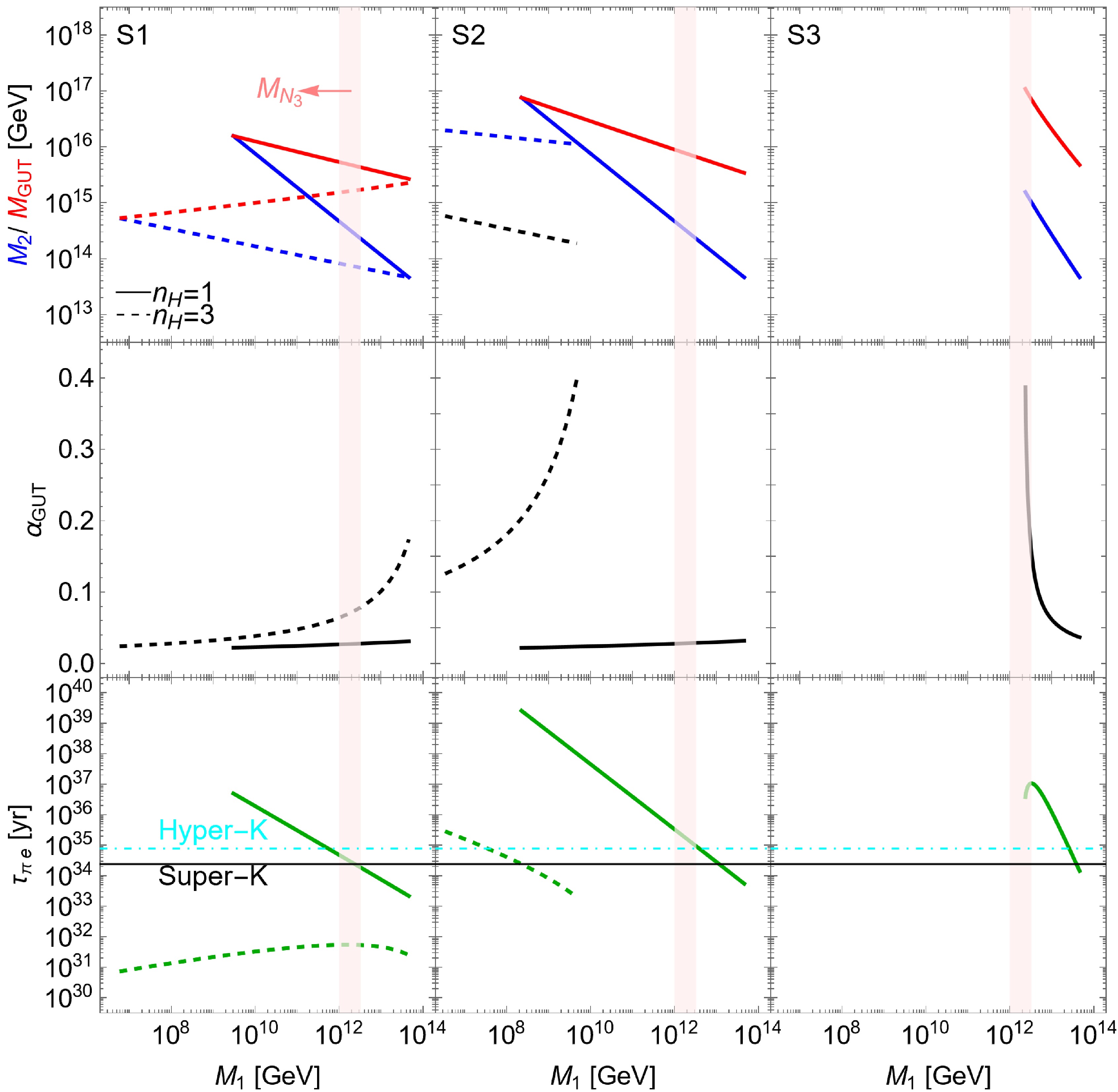

Figure 3.  (color online) Predictions of GUT scale $M_{\rm{GUT}}$, intermediate scales, $M_1$ and $M_2$, gauge coupling at GUT scale $\alpha_{\rm{GUT}}$, and partial lifetime for proton decaying to $\pi^0 e^+$ in three scenarios: S1 (left), S2 (middle), and S3 (right). The energy scale hierarchy $M_1 \leq M_2 \leq M_{\rm{GUT}}$ is required; $n_H = 1$ (solid curve) and 3 (dashed curve) refer to the repetition number of the Higgs fields ${\bf{10}}_H,{\overline{\bf{126}}}_H,{\bf{120}}_H${the predicted range of $M_{N_3}$ in the last section is represented in the pink band as a reference}. S3 presents no solution for $n_H = 3$ ; therefore, it is not shown in the right panel.

In conclusion, we should be careful about adding Higgs fields, as an increased number of Higgs fields implies a faster evolution of the gauge couplings, which may increase excessively, a situation not favored theoretically. When $ n_H = 1 $, the above three scenarios restrict $ M_1 $, which should be smaller than $ 4.6\times 10^{13} $ GeV, consistent with $ M_{N_3}<4.4\times 10^{13} $ GeV in Refs. [25, 52]. Furthermore, viable points of $ \chi^2\leq10 $ in our model always meet this requirement.

In non-SUSY $ S O(10) $ GUTs, proton decay will be induced by integrating out the superheavy gauge fields $ ({{\bf{3}},{\bf{2}}},-\dfrac{5}{6}),({ \overline{{\bf{3}}},{\bf{2}}},\dfrac{5}{6}),({{\bf{3}},{\bf{2}}},\dfrac{1}{6}),({ \overline{{\bf{3}}},{\bf{2}}},-\dfrac{1}{6}) $, which are typically denoted as $ X^\mu,Y^\mu,X^{\prime\mu},Y^{\prime\mu} $, resulting in the following four dimension-six operators [53]:

where $ i,j,k $ ($ \alpha,\beta $) denote color (flavor) indices and $ \Lambda_{1}\simeq \sqrt{2}M_{(X,Y)}/g_{\rm{GUT}},~~ \Lambda_{2}\simeq \sqrt{2}M_{(X^\prime,Y^\prime)}/g_{\rm{GUT}} $ are the UV completion scales of the GUT symmetry. These four operators trigger proton decay in the form $ p\rightarrow M+\overline{l} $, where mesons M can be $ \pi^0,\pi^+,K^0,K^+,\nu $ and leptons l can be $ e,\mu,\nu $ [54]. The partial decay width for such decay mode can be written as [55, 56]

where $ n = L,R $, $ m_p $ and $ m_M $ are masses of proton and mesons, $ W_n $ denotes the Wilson coefficients of the operators in Eq. (56) that give rise to a specific decay channel, $ F_0^n = \langle M | (qq^\prime)_{L,R} q^{\prime\prime}_L | p \rangle $ is the revelant hadronic matrix element, and $ q,q^\prime,q^{\prime\prime} = u,d,s $.

Furthermore, $ A_L $ represents the long range effect from the proton scale ($ m_p\sim 1 $ GeV) to electroweak scale ($ M_Z $) calculated at the two-loop level $ A_L = 1.247 $ [57, 58]. $ A_{SL} $ and $ A_{SR} $ represent the short range effects obtained from RG running from $ M_Z $ to the GUT scale $ M_{\rm{GUT}}\simeq M_{(X,Y)} = M_{(X^\prime,Y^\prime)} $. Therefore, these two factors non-trivially depend on the breaking chain. $ A_{SL} $ and $ A_{SR} $ are given by [59−62]

where $ \gamma_i $ and $ b_i $ denote the anomalous dimension and one-loop β coefficient, respectively, and $ \gamma_i $ at given intermediate scales can be found in [52].

We focus on the golden channel $ p\rightarrow\pi^0e^+ $, given that $ \Lambda_{1}\simeq\Lambda_{2}\simeq \sqrt{2}M_{\rm{GUT}}/g_{\rm{GUT}} $. The decay widths of this channel can be expressed as

An analysis of the fermion masses and mixing allowed us to determine each unitary matrix in this formula for each point in Fig. 1. In particular, as Yukawa coupling matrices are Hermitian in our model, we have $ U_u^\prime = U_u = P_uO_u, U_d^\prime = U_d = P_dO_d, \; U_e^\prime = U_e $, and $ U_e $ can be derived throgh diagonalization $ U_e^\dagger Y_e U_e = \text{diag}\{y_e,y_\mu,y_\tau\} $. Once we substitute the numerical results in Eq. (59), the proton decay lifetime of $ p\rightarrow\pi^0e^+ $ is only proportional to $ \dfrac{4M_{\rm{GUT}}^4}{g_{\rm{GUT}}^4} = \Big(\dfrac{M_{\rm{GUT}}^2}{2\pi\alpha_{\rm{GUT}}}\Big)^2 $. Predictions for the proton decay lifetime in this channel for the aforementioned three scenarios are shown in Fig. 3. Here, we observe that the effect of the flavor part $ U_u,U_d,U_e $ in Eq. (59) is small, and the difference between the maximum and minimum values of the proton decay lifetime corresponding to the same $ M_1 $ value is within 5%. As $ n_H $increases, or equivalently, if more Higgs fields are added, the proton decay lifetime decreases owing to the increase in $ \alpha_{\rm{GUT}} $. In scenario 2, we add $ ({{\bf{6}},{\bf{1}},{\bf{1}}})\subset {\bf{10}}_H $ in $ G_{422}^{\rm{C}} $ and its decomposition $ ({{\bf{3}},{\bf{1}},{\bf{1}}},-\dfrac{1}{3}),({\overline{{\bf{3}}},{\bf{1}},{\bf{1}}},\dfrac{1}{3})\subset {\bf{10}}_H $ in $ G_{3221} $ to improve the GUT scale, and its proton decay lifetime can exceed the future Hyper-Kamiokande (HK) target of $ \tau_{\pi^0e^+}>7.8\times 10^{34} $ years [49] even when $ n_H = 3 $. However, the maximum of the lowest intermediate scale $ M_1 $ allowed by the Super-Kamiokande (SK) bound decreases to $ 2.3\times 10^{8} $ GeV, which is smaller than $ M_{N_3} $ in Fig. 2. When $ n_H = 1 $, all three scenarios satisfy the SK bound $ \tau_{\pi^0e^+}>2.4\times 10^{34} $ years [63]; the constraints on $ M_1 $ for three scenarios are S1: $ M_1\leq 2.6 \times 10^{12} $ GeV, S2: $ M_1\leq 1.2 \times 10^{13} $ GeV, and S3: $ M_1\leq 3.9 \times 10^{13} $ GeV. It is clear that the predicted range of $ M_{N_3} $ in Fig. 2 consistently satisfies this requirement.

We have proposed a UTZT, implying that all $ 3\times 3 $ fermion Yukawa/mass matrices take two-zero flavor textures, in the $ S O(10) $ GUT framework to restrict the flavor space of quarks and leptons. Through a concrete example, we show that the UTZT flavor structure can be realized in a $ Z_6 $ flavor symmetry. The quark and lepton mass matrices are all correlated with each other owing to the grand unification. The light neutrino mass matrix, generated via the Type-I+II seesaw mechanism, is shown to maintain the UTZT property. Together with the relation between the Dirac Yukawa coupling matrices in Eq. (5), we explored seven free parameters to fit nine observables (three mixing angles and one CP-violating phase in the quark sector, three mixing angles, and two mass-squared differences in the lepton sector). The leptonic CP-violating phase was treated as a prediction in the range $ (90^\circ, 230^\circ) $. The upcoming long-baseline neutrino experiments will have the potential to exclude part of the parameter space. Our exploration results show that the right-handed neutrino spectrum can be strongly constrained, given that the model must fit all flavor data, including fermion masses, CKM mixing, and PMNS mixing. The heaviest right-handed neutrino mass is predicted to be less than $ 3.3 \times 10^{12} $ GeV, which is allowed by gauge unification and proton decay measurements in non-SUSY $ S O(10) $ GUTs. The predicted region of $ m_{ee} $ vs $ m_1 $ in Fig. 2 for neutrinoless double beta decay experiments will allow us to test the grand unification.

We performed the gauge unification for a specific breaking chain with two intermediate scales and examined the range of allowed intermediate scales. The color triplet Higgses of $ S U(3)_c $, which are decomposed from sextet of $ S U(4)_c $ and further decomposed from $ {\bf{10}}_H $ of $ S O(10) $, were found to improve the GUT scale but decrease the lowest intermediate scale. The Higgs bi-doublets of $ S U(2)_L \times S U(2)_R $ can improve the lowest intermediate scale but reduce the GUT scale. Therefore, we assume a few copies of Higgs bi-doublets at low energy, leading to an improvement of the GUT scale. When $ n_H = 1 $, or equivalently, without adding too many Higgs fields, all three aforementioned scenarios require that the maximum of the lowest intermediate scale $ M_1 $ be less than $ 4.6\times 10^{13} $ GeV, which is consistent with predicted observables of this model in Fig. 2. Adding too many Higgs fields causes gauge coupling at the GUT scale to become too large, which should be considered carefully. Proton decay is also discussed. As long as too many Higgs fields are not added, the gauge coupling at the GUT scale will not become very large, i.e., $ \alpha_{\rm{GUT}}\in(0.022, 0.032) $. Therefore, the GUT scale is always high enough to meet the SK bound, i.e., approximately $ M_{\rm{GUT}}\ge 4.5\times 10^{15} $ GeV.

The authors would like to thank Z.-z. Xing and D. Zhang for useful discussions in the initial stage of this study.

Next, we check the validity of Eq. (5) when $ {\bf{10}}_H $ and $ {\bf{120}}_H $ are complex. The copies of $ {\bf{10}}_H $, $ \overline{\bf{126}}_H $, and $ {\bf{120}}_H $ satisfy $ n > 1 $. We start with the most general form of Yukawa terms in $ S O(10) $,

where $ k = 1,2,..., n $. The $ A'_k $ and $ C'_k $ terms are forbidden if the Peccei-Quinn (PQ) symmetry is imposed; $ {\bf{10}}_H $, $ {\bf{120}}_H $, $ \overline{\bf{126}}_H $ are decomposed into a series of electroweak doublets in the SM gauge symmetry, and these doublets mix together. Up to now, we have a total of $ 8n $ pairs of Higgs doublets,

where superscripts $ 1 $ and $ 2 $ of $ 120_H^{u} $ and $ 120_H^{d} $ denote the SU(4) singlet and adjoint representation under the $ G_{422} = S U(4)_c\times S U(2)_L\times S U(2)_R $ decomposition. The Yukawa terms after decomposition are explicitly expressed as

It is convenient to rotate the interaction basis h to the mass basis $ \hat{h} $ via a unitary transformation,

where ${ \widetilde{h_u}} = { i} \sigma_2 h_u^{*} $, W is a unitary matrix, the subscript for mass states $ i = 1,2,..., 8n $ is arranged following the mass ordering, and the subscript for interaction states $ a = j_k $ is further split into two subscripts, $ j = 1,2,...8 $ and $ k = 1,2, ..., n $, with respect to the copy for $ n>1 $. In the minimal case, only the SM Higgs $ h_{\rm{SM}} \equiv \hat{h}_1 $, which is the massless Higgs doublet before electroweak symmetry breaking, contributes to fermion masses. Then, we decompose Yukawa couplings in Eq. (62) into its SM parts and obtain terms of fermion masses:

Based on these terms, we can parameterize the Dirac Yukawa coupling matrices of fermions into a more concise form:

where

If the PQ symmetry is imposed, $ A'_k $ and $ C'_k $ are forbidden, and we obtain Eq. (5). If $ A'_k $ and $ C'_k $ are present and $ r_1,r_3,c_e,c_\nu $ are real numbers, Eq. (65) is simplified as

We obtain the same form as that of Eq. (5) again. In fact, when we introduce $ {\bf{10}}_H $, $ \overline{\bf{126}}_H $, $ {\bf{120}}_H $ to generate fermion masses, given that $ ({\bf{1}},{\bf{2}},{\bf{2}})\in {\bf{10}}_H,{\bf{120}}_H $ and $ ({\bf{15}},{\bf{2}},{\bf{2}})\in {\bf{120}}_H,\overline{{\bf{126}}}_H $ are responsible for electroweak symmetry breaking and yield fermion masses, these four Higgs fields only lead to a total of eight independent terms in Yukawa coupling matrices: four terms $ W_{1,1_k} A^*_k+W^*_{1,1_k} A^{\prime *}_k, W_{1,4_k} B^*_k, ~~W_{1,2_k} C^*_k+W^*_{1,2_k} C^{\prime *}_k, ~~W_{1,3_k} C^*_k+W^*_{1,3_k} C^{\prime *}_k $ in $ Y_u,Y_\nu $ and four terms $ W^*_{1,5_k} A^*_k+W_{1,5_k} A^{\prime *}_k, ~~W^*_{1,8_k} B^*_k $, $ W^*_{1,6_k} C^*_k+ W_{1,6_k} C^{\prime *}_k, ~~W^*_{1,7_k} C^*_k+W_{1,7_k} C^{\prime *}_k $ in $ Y_d,Y_e $.

The discussion can also be extended to the case of more Higgses evolving in the fermion masses. For example, in the two-Higgs-doublet model (THDM), by denoting the two light Higgses as $ \hat{h}_1 = W_{1,a}h_a,\hat{h}_2 = W_{2,a} h_a $, the aforementioned eight terms can be rewritten by replacing $ W^*_{1,j_k} $ with certain combinations of $ W^*_{1,j_k} $ and $ W^*_{2,j_k} $, which will not be repeated here.

In the case of real $ {\bf{10}}_H $ and $ {\bf{120}}_H $, $ {\bf{10}}_H^* $ is identical to $ {\bf{10}}_H $, and so is $ {\bf{120}}_H $. Terms of $ A',C' $ can be absorbed into terms of A and C, respectively; in addition, $ \widetilde{10_{Hk}^u} = 10_{Hk}^d $, $ \widetilde{120_{Hk}^{u1}} = 120_{Hk}^{d1} $, and $ \widetilde{120_{Hk}^{u2}} = 120_{Hk}^{d2} $. The total number of copies of doublets is reduced to $ 5n $, and thus, the subscript a denotes $ 1_k, 2_k, ..., 5_k $.

Among all points in our exploration, we found that the minimal value of $ \chi^2 $ is 1.6. Inputs and predictions of fermion Yukawa matrices and mixing parameters are shown in Table B1. Yukawa matrices H, F, and G at this point are given by

Inputs	$A_u$	$A_d$	$\phi_1$	$\phi_2$
	0.3665	0.0048	4.7379	1.4232
	$c_\nu$	$m_L$	$m_R$
	0.0940	13.8057 eV	0.5588 eV
	$(\eta_u,\eta_d,\eta_e,\zeta_d)$
	(+, +, –, –)
Outputs	$\theta_{12}^q$	$\theta_{23}^q$	$\theta_{13}^q$	$\delta^q$
	$13.0356^\circ$	$2.8011^\circ$	$0.2366^\circ$	$67.04^\circ$
	$\theta_{12}^l$	$\theta_{23}^l$	$\theta_{13}^l$	$\delta^l$
	$33.26^\circ$	$48.52^\circ$	$8.55^\circ$	$160^\circ$
$\chi^2=1.6$	$m_1$	$\Delta m_{21}^2$	$\Delta m_{31}^2$	$\left\langle m \right\rangle _{ee}$
	0.491 meV	$7.44 \cdot 10^{-5}$	$2.509 \cdot 10^{-3}$	3.98 meV
	$M_{N_1}$	$M_{N_2}$	$M_{N_3}$	$\mathcal{J}$
	$1.07 \cdot 10^{10} \, \rm GeV$	$2.93 \cdot 10^{11} \, \rm GeV$	$2.96 \cdot 10^{12} \, \rm GeV$	1.14%

Table B1.  Inputs and predictions of neutrino masses and mixing parameters for minimal $\chi^2$ in our exploration. Charged fermion masses are all fixed at experimental best-fit values. Neutrino masses with normal ordering are predicted.

respectively. Accordingly, all charged fermion Yukawa matrices and the light neutrino mass matrix are obtained:

Then, applying the inverse of the Type-(I+II) seesaw formula, the right-handed neutrino mass matrix becomes

Three RH neutrino masses were predicted to be on orders of $ 10^{10} $, $ 10^{11} $, and $ 10^{12} $ GeV. In particular, the heaviest right-handed neutrino mass is $ 2.96 \times 10^{12} $ GeV, which is below the $ B-L $ breaking scale, $ M_{B-L} \simeq 4.6 \times 10^{13} $ GeV $ (n_H = 1) $ , and thus consistent with proton decay measurements.